Ranking the information content of distance measures

Abstract

Real-world data typically contain a large number of features that are often heterogeneous in nature, relevance, and also units of measure. When assessing the similarity between data points, one can build various distance measures using subsets of these features. Finding a small set of features that still retains sufficient information about the dataset is important for the successful application of many statistical learning approaches. We introduce a statistical test that can assess the relative information retained when using two different distance measures, and determine if they are equivalent, independent, or if one is more informative than the other. This ranking can in turn be used to identify the most informative distance measure and, therefore, the most informative set of features, out of a pool of candidates. To illustrate the general applicability of our approach, we show that it reproduces the known importance ranking of policy variables for Covid-19 control, and also identifies compact yet informative descriptors for atomic structures. We further provide initial evidence that the information asymmetry measured by the proposed test can be used to infer relationships of causality between the features of a dataset. The method is general and should be applicable to many branches of science.

In real-world data sets many characteristics are often associated with each data point, and one can imagine different ways to define the similarity between two samples. For example, in a clinical database two patients might be compared based on their age, sex, or height, or on the results of specific clinical exams. In this work we introduce a method which allows studying the relationship between different distances (or similarity) measures defined on the same dataset. One can find that two distances are unrelated, that they bring equal information, or that one of the two distances allows predicting the other, while the reverse is not true. This allows finding distances which are maximally informative for a prediction, and detecting causality relationships.

1 Introduction

An open challenge in machine learning is to extract useful information from a database with relatively few data points, but with a large number of features available for each point Wang et al. (2020); Lopes et al. (2017); Nazábal et al. (2020). For example, clinical databases typically include data for a few hundreds patients with a similar clinical history, but an enormous amount of information for each patient: the results of clinical exams, imaging data, and a record of part of their genome Sudlow et al. (2015). In cheminformatics and materials science, molecules and materials can be described by a large number of features, but databases are limited in size by the great cost of the calculations or the experiments required to predict quantum properties Altae-Tran et al. (2017); Yamada et al. (2019). In short, real-world data are often “big data”, but in the wrong direction: instead of millions of data points, there are often too many features for a few samples. As such, training accurate learning models is challenging, and even more so when using deep neural networks, which typically require a large amount of independent samples Shorten and Khoshgoftaar (2019).

One way to circumvent this problem is to perform preliminary feature selection, and discard features that appear irrelevant or redundant Cai et al. (2018); Lopes et al. (2017); Jović et al. (2015); Deng et al. (2019). Alternatively, one can perform a dimensional reduction aimed at finding a representation of the data with few variables built as functions of the original features van der Maaten and Hinton (2008); McInnes et al. (2018); Bengio et al. (2013).

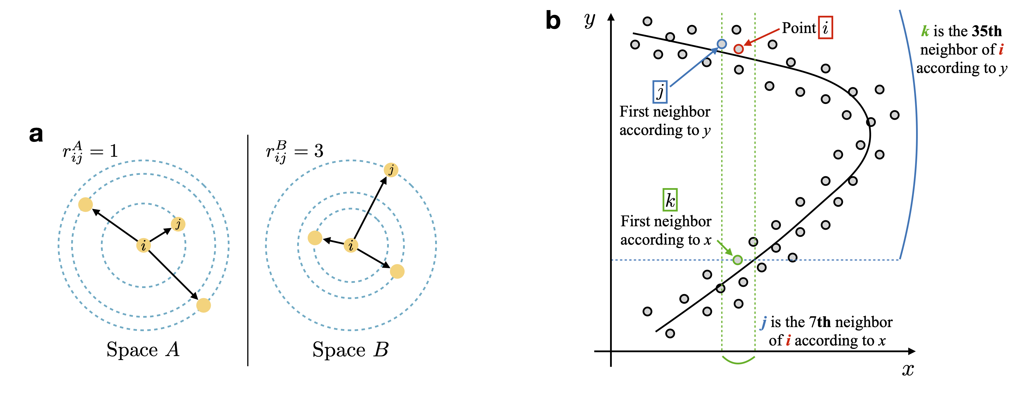
Figure 1: Distance ranks can be used to measure the relative informations contained in two distance measures. a): Illustration of the distance rank of two points in different feature spaces $A$ and $B$. The rank $r_{ij}$ of point $j$ relative to $i$ is equal to 1 in space $A$, meaning that $j$ is the first neighbor of $i$. This is not the case in space $B$, where point $j$ is the third neighbor of point $i$. b): Illustration of how ranks can be used to verify that space $x$ is less informative than space $y$. The figure shows how a distance bound in $y$ automatically implies a distance bound in $x$. The opposite is not necessarily true: the first neighbor of a point in the $x$ space can be very far in $y$.

In some cases, explicit features are not available, as in the case of raw text documents or genome sequences. What one can always define, even in these cases, are distances between data points whose definition, however, can be rather arbitrary Kaya and Bilge (2019); Kulis (2013). How can one select, among an enormous amount of possible choices, the most appropriate distance measure for a given task? Finding the correct distance is of course as difficult as performing feature selection or dimensionality reduction. In fact, these tasks can be considered equivalent if explicit features are available, since in this case a particular choice of features naturally gives rise to a different distance function computed through the Euclidean norm.

In this work, we approach feature/distance learning through a novel statistical and information theoretic concept. We pose the question: given two distance measures $A$ and $B$, can we identify whether one is more informative than the other? If distance $A$ is more informative than distance $B$, even partial information on the distance $A$ can be predictive about $B$, while the reverse will not necessarily be true. If this happens, and if the two distances have the same complexity e.g, they are built using the same number of features, $A$ should be generally preferred with respect to $B$ in any learning model.

We introduce the concept of “information imbalance”, a measure able to quantify the relative information content of one distance measure with respect to another. We show how this tool can be used for feature learning in different branches of science. For example, by optimizing the information content of a distance measure we are able to select from a set of more than 300 material descriptors, a subset of around 10 which is sufficient to define the state of a material system, and predict its energy. Moreover, we use the information imbalance to verify that the national policy measures implemented to contain the Covid-19 epidemic are informative about the future state of the epidemic. In this case, we also show that the method can be used to detect causality relationship between variables.

2 The information imbalance

Inspired by the widespread idea of using local neighborhoods to perform dimensional reduction Hastie et al. (2001) and classification Gashler et al. (2008) we quantify the relative quality of two distance measures by analyzing the ranks of the first neighbors of each point. For each pair of points $i$ and $j$, the rank $r_{ij}$ of point $j$ relative to point $i$, is obtained by sorting the pairwise distances between $i$ and rest of the points from smallest to largest. For example, $r_{ij}^{A}=1$ if point $j$ is the first neighbor of point $i$ according to the distance $d_{A}$. The rank of two points will be, in general, different when computed using a different distance measures $B$, as illustrated in Figure 1a.

The key idea of our approach is that distance ranks can be used to identify whether one metric is more informative than the other. Take the example given in Figure 1b, depicting a schematic representation of a noisy curved dataset. In this dataset the distance along the $y$-axis is clearly more informative than the one along the $x$-axis since one could construct a function able to predict $x$ from the knowledge of $y$, but not the opposite. This asymmetry is well captured by the ranks between points. Take for example point $i$ (red circle in the figure). Its first neighbour according to the $y$-distance is $j$ (blue circle), while according to the $x$-distance (green lines) $j$ is the 7th neighbour of $i$ . Conversely, the nearest neighbour of $i$ according to the $x$-distance is $k$ (green circle), which is the 35th neighbour of $i$ according to the $y$-distance (blue lines). We hence find that $r_{ij}^{x}\ll r_{ik}^{y}$ i.e., the rank in space $x$ of the first neighbor measured in space $y$ is much smaller than the rank in space $y$ of first neighbor measured in space $x$.

To give a more quantitative example, let’s consider a dataset of points harvested from a 3-dimensional Gaussian whose standard deviation along the $z$ direction is a tenth of those along $x$ and $y$. In this case, one can define a Euclidean distance between data points either using all the three features, $d_{xyz}^{2}=(x_{i}-x_{j})^{2}+(y_{i}-y_{j})^{2}+(z_{i}-z_{j})^{2}$, or using a subset of these features ( $d_{xy}$, $d_{yz}$ and so on).

Intuitively, $d_{xyz}$ and $d_{xy}$ are almost equivalent since the standard deviation along $z$ is small, while there are information imbalances, say, between $d_{x}$ and $d_{xy}$, which would allow saying that $d_{xy}$ is more informative than $d_{x}$.

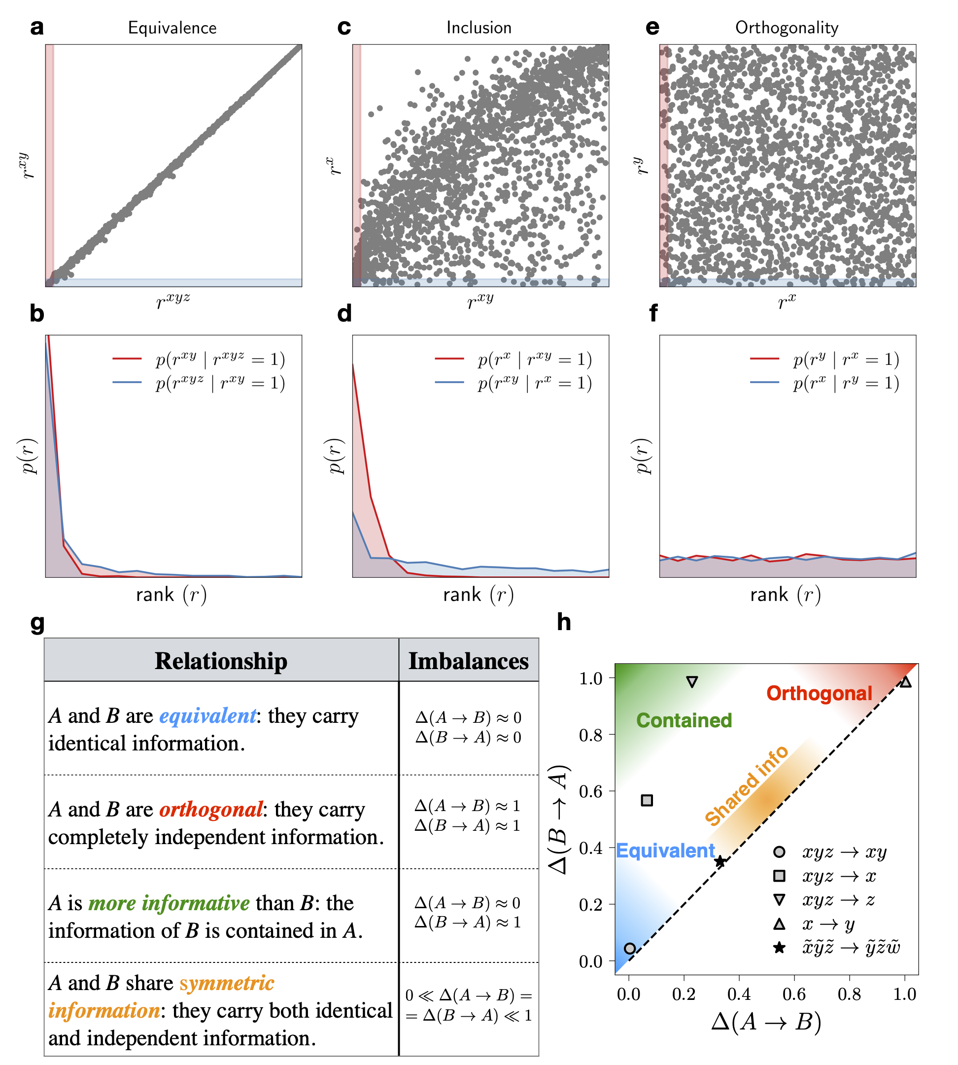
Figure 2: Classifying and visualizing the relationship between any two distance measures using the information imbalance. a), c), e): Scatter plots of the ranks between ordered pairs of points for different distance measures evaluated on a 3D Gaussian dataset with a small variance along $z$. The red and blue bands indicate, respectively, the points for which the rank on the $x$ and $y$ axis is equal to one (proportions were exaggerated for clarity). The histogram of the points inside each band is plotted in the bottom plots using the same color. b), d), f): Probability of that two nearest neighbor points ($r=1$) for one distance have rank $r$ for the other distance. The three columns represent different pairs of representations. g): The four different types of relationships that can characterize the relative information content of two spaces $A$ and $B$. h): Information imbalance plane for the discussed 3D Gaussian dataset with small $z$-axis variance (gray markers), and for a 4D isotropic Gaussian dataset (black star). The different colors (light blue, red, green and orange) roughly mark the regions corresponding to the four types of relationships listed in panel g.

In the first row of Figure 2, we plot the ranks computed using one distance against the ranks computed using a second distance (for example the ranks in $d_{xy}$ as a function of those in $d_{xyz}$ for panel a). In the second row of the figure we show the probability distribution $p(r^{A}\mid r^{B}=1)$ of the ranks $r_{ij}^{A}$ in space $A$ restricted to those pairs $(i,j)$ for which $r_{ij}^{B}=1$, namely to the nearest neighbors according to distance $B$. In panels a and b, we compare the most informative distance containing all three coordinates to the one containing only the $x$ and $y$ coordinates. Given the small variance along the $z$ direction, these two distance measures are practically equivalent, and this results in rank distributions strongly peaked around one. In panels c and d, we compare the two metrics $d_{xy}$ and $d_{x}$. In this case, the former is clearly more informative than the latter, and we find that the distribution of ranks when passing from $d_{xy}$ to $d_{x}$ is more peaked around small values than when going in the opposite direction. Finally, for two metrics built using independent coordinates ($x$ and $y$, in panels c and f) the rank distributions are completely uniform.

We hence propose to assess the relationship between any two distance measures $d_{A}$ and $d_{B}$ by using the properties of the conditional rank distribution $p(r^{B}\mid r^{A}=1)$. The closer this distribution is to a delta function peaked at one, the more information about space $B$ is contained within space $A$.

This intuition can be made more rigorous through the statistical theory of copula variables. We can define a copula variable $c_{A}$ as the cumulative distribution $c_{A}=\int_{0}^{d_{A}}p_{A}(w\mid x)dw$, where $p_{A}(w\mid x)$ is the of probability of sampling a data point within distance $w$ from $x$ in the $A$ space. The value of $c_{A}$ can be estimated from a finite dataset by counting the fraction of points that fall within distance $d_{A}$ of point $x$, $c_{A}\approx r_{A}/N$. Copula variables and distance ranks can be considered continuous-discrete analogues of each other. As a consequence, the distributions $p(r^{B}\mid r^{A}=1)$ shown in Figure 2 are nothing else but estimates of the copula distributions $p(c_{B}\mid c_{A})$ with $c_{A}$ conditioned to be very small. This is important, since Sklar’s theorem guarantees that the copula distribution $p(c_{A},c_{B})$ contains the entire correlation structure of the metric spaces $A$ and $B$, independently of any details of the marginal distributions $p(d_{A}\mid x)$ and $p(d_{B}\mid x)$ Nelsen (2006); Calsaverini and Vicente (2009); Safaai et al. (2018).

Using the copula variables, we define the “information imbalance” from space $A$ to space $B$ as

$$\Delta(A\rightarrow B)=2\lim_{\epsilon\rightarrow 0}\,\langle c_{B}\mid c_{A}=\epsilon\rangle,$$ (1)

where we used the conditional expectation $\langle c_{B}\mid c_{A}=\epsilon\rangle=\int c_{B}\,p(c_{B}\mid c_{A}=\epsilon)dc_{B}$ to characterize the deviation of $p(c_{B}\mid c_{A}=\epsilon)$ from a delta function. In the limit cases where the two spaces are equivalent or completely independent we have that $\langle c_{B}\mid c_{A}=\epsilon\rangle=\epsilon$ and $\langle c_{B}\mid c_{A}=\epsilon\rangle=1/2$ respectively, so that the definition provided in Eq. (1) statistically confines $\Delta$ in the range $(0,1)$. The information imbalance defined in Eq. (1) is estimated on a dataset with $N$ data points as

$$\Delta(A\rightarrow B)\approx 2\langle r^{B}\mid r^{A}=1\rangle/N$$ (2)

We remark that the conditional expectation used in Eq. (1) is only one of the possible quantities that can be used to characterize the deviation of the conditional copula distribution from a delta function. Another attractive option is the entropy of the distribution. In the Supplementary Material (SM) (S1.C), we show how these two quantities are related and we demonstrate that the specific choice does not substantially affect the results. In the SM (see S1.B and Figure S1), we also show how copula variables can be used to connect the information imbalance to the standard information theoretic concept of mutual information.

By measuring the information imbalances $\Delta(A\rightarrow B)$ and $\Delta(B\rightarrow A)$, we can identify four classes of relationships between the two spaces $A$ and $B$. We can find whether $A$ and $B$ are equivalent or independent, whether they symmetrically share both independent and equivalent information, or whether one space contains the information of the other. These relationships are presented in Figure 2g. These relationships can be identified visually by plotting the two imbalances $\Delta(A\rightarrow B)$ and $\Delta(B\rightarrow A)$ against each other in a graph as done in Figure 2h. We will refer to this kind of graphs as information imbalance planes. In Figure 2h we present the information imbalance plane of the 3-dimensional Gaussian dataset discussed so far, and used for Figure 2a-f. Looking at this figure, one can immediately verify that the small variance along the $z$ axis makes the two spaces $xyz$ and $xy$ practically equivalent (gray circle). Similarly, one can verify that space $x$ is correctly identified to be contained in $xyz$ (gray square) and that the two spaces $x$ and $y$ are classified as orthogonal (gray triangle). The figure also includes a point corresponding to a different dataset sampled from a 4-dimensional isotropic Gaussian with dimensions $\tilde{x}$, $\tilde{y}$, $\tilde{z}$ and $\tilde{w}$. This point (black star) shows that the spaces $\tilde{x}\tilde{y}\tilde{z}$ and $\tilde{y}\tilde{z}\tilde{q}$ are correctly identified as sharing symmetric information. Importantly, the information imbalance only depends on the local neighborhood of each point and, for this reason, it is naturally suited to analyze data manifolds which are arbitrarily nonlinear. In the SM (see S2.A and Figure S2), we show that our approach is able to correctly identify the best feature for describing a spiral of points wrapping around one axis, and a sinusoidal function. More numerical tests are available online at DAD (2022) along with the corresponding code Glielmo et al. (2022). In the examples discussed so far we have chosen the Euclidean metric as distance measure for any subset of coordinates considered. We will make the same choice throughout the rest of this work.

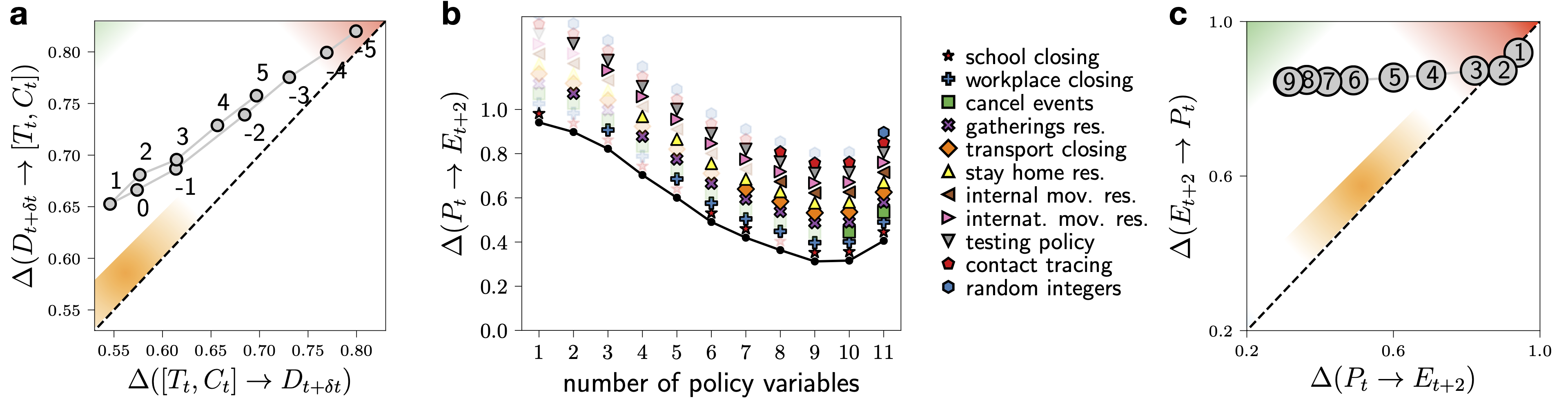
Figure 3: The information imbalance allows for a straightforward verification of the impact of national policy measures on the Covid-19 epidemic. a) Information imbalance between the space $[T_{t},C_{t}]$ of the number of tests and number of confirmed cases $C_{t}$ in a given week $t$, and the number of deaths $D_{t+\delta t}$ occurred in week $t+\delta t$. The time shift $\delta t$ ranges from $-5$ (5 weeks before) to $+5$ (5 weeks after). b): Minimum information imbalances from growing sets of policy variables $P_{t}$ to the state of the epidemic after two weeks $E_{t+2}$. c): The corresponding information imbalance plane with the number of policy variables going from 1 to 10 reported in the gray circles. Point 10 is not visible as it lies below point 9. The figure shows that the policy measures space $P_{t}$ can predict the state of the epidemic $E_{t+2}$, while $E_{t+2}$ cannot predict $P_{t}$.

3 Influence of national policy measures on the Covid-19 epidemic

We now use the information imbalance to analyze the “Covid-19 Data Hub”, a dataset which provides comprehensive and up to date information on the Covid-19 epidemic Guidotti and Ardia (2020), including epidemiological indicators such as the number of confirmed infections and the number of Covid-19 related deaths for nations where this is available, as well as the policy indicators that quantify the severity of the governmental measures such as school and workplace closing, restrictions on gatherings and movements of people, testing and contact tracing Hale et al. (2020). More details on the dataset are available in the SM (S2.B.1).

We first illustrate how the information imbalance can be used to recover the arrow of time from time series data. In Figure 3a we show the information imbalance between the space $[T_{t},C_{t}]$, containing the number of tests $T_{t}$ and the number of confirmed cases $C_{t}$ in a given week $t$, and the space of the number of deaths occurring in week $t+\delta t$ ($D_{t+\delta t}$). The imbalance is shown as a function of $\delta t$. All the points lay above the diagonal, indicating that, in the language of Figure 2h, the number of deaths is marginally contained in the two variables $[T_{t},C_{t}]$ if $\delta_{t}$ is small; and the optimal information imbalance occurs at $\delta t=1$. Importantly, for each pair of opposite time lags ($\delta t,-\delta t$) we find that the two variables $[T_{t},C_{t}]$ always contain more information on future deaths than on past deaths. In this scenario this result represents an obvious verification of the known arrow of time of the dataset, but it suggests that further dedicated investigations could bring to the development of accurate tests to detect nontrivial causality relationships Runge et al. (2019).

We now analyze the relationship between the space of policy measures $P_{t}$ at week $t$, and the state of the epidemic $E_{t+\delta t}$, with $\delta t=2$ (namely after two weeks). In SM (S2.B.2, Figure S3) we show that the analysis with time lags of one or three weeks bring to similar results. While we consider several different choices for the policy space, the epidemic state is defined by the number of weekly deaths $D_{t}$ and the ratio $R_{t}=C_{t}/T_{t}$ of confirmed cases $C_{t}$ over total number of tests performed $T_{t}$ per week. We estimate the information imbalance $\Delta(P_{t}\rightarrow E_{t+\delta t})$ between the spaces defined by all the possible combination of policy measures $P_{t}$ and the space of epidemiological variables $E_{t+\delta t}$. A low value of $\Delta(P_{t}\rightarrow E_{t+\delta t})$ means that $P_{t}$ can predict $E_{t+\delta t}$. In Figure 3b we present the minimum information imbalance $\Delta(P_{t}\rightarrow E_{t+\delta t})$ achievable with any set of $d$ policy measures.

For $d\leq 2$, $\Delta(P_{t}\rightarrow E_{t+\delta t})$ is close to one, indicating that no single or couple of policy measure is significantly predictive about the state of the epidemic, consistently with Haug et al. (2020). When three or more policy measures are considered, the information imbalance decreases rapidly reaching a value of about $0.28$ when almost all policy measures are considered. This sharp decrease and the low value of the information imbalance clearly indicate that policy measures do contain information on the future state of the epidemic, and the more policy measures are considered, the more the future state of the epidemic can be considered as contained in the space of the policies. As a sanity check, a dummy policy variable was introduced for this test (blue hexagon). This variable is never selected by the algorithm, and its addition deteriorates the information content of the policy space.

The described analysis verifies that policy interventions have been effective in containing the spreading of the Covid-19 epidemic, a result which has been shown in a number of studies Brauner et al. (2021); Haug et al. (2020); Hsiang et al. (2020); Flaxman et al. (2020). In accordance with these studies, we also find that multiple measures are necessary to effectively contain the epidemic, with no single policy being sufficient on its own Soltesz et al. (2020), and that the impact of policy measures increases monotonically with the number of measures put in place. We find that a small yet effective set of policy measures has been the combination of testing, stay home restrictions and restrictions on international movement and gatherings. While our results are computed as averages over all nations considered, further analysis carried out in the SM (S2.B.3, Figure S5) on disjointed subsets of nations give results which are consistent with our main findings.

We finally note that the information imbalance $\Delta(E_{t+2}\rightarrow P_{t})$ (shown in Figure 3c) remains considerably high for any number of policy variables. This indicates that the state of the epidemic is not informative about past policy measures. Surprisingly, the state of the epidemic is not informative even on future policy measures (see S2.B.2 and Figure S4 of the SM), a result which seems to indicate that that different nations have reacted to the epidemic through widely different strategies.

The information imbalance can also be used to optimally choose the relative scale of heterogeneous variables. For instance, in the SM (S2.B.4, Figure S6), we use the information imbalance to select the relative scale of heterogeneous epidemiological variables such as the total number of tests and the ratio of confirmed cases over total number of tests. This is important in real-world applications, where features are often characterized by different units of measure and different scales of variations.

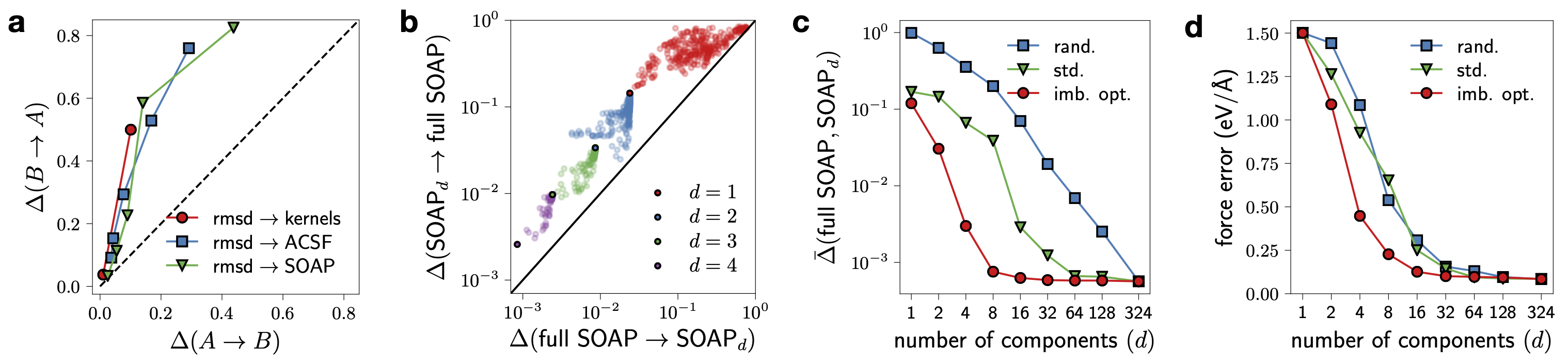
Figure 4: The information imbalance can be used to perform an effective information-driven feature selection in materials systems. a): Information imbalances between ground truth “rmsd” distance metric and standard atomistic descriptors. b): Information imbalances between a full description and the most informative $d$-plet of components ($d=1,\dots,4$). c): Convergence of the “symmetric” information imbalance with the number of components for three different compression strategies. The symmetric information imbalance is defined as $\bar{\Delta}(A,B)=[\Delta(A\rightarrow B)+\Delta(B\rightarrow A)]/\sqrt{2}$; more details can be found in the SM (S2.C.3). d): Force error on a validation set of a machine learning potential energy model built on the compressed descriptors.

4 Selection and compression of descriptors in materials physics

We now show that the information imbalance criterion can be used to assess the information content of commonly used numerical descriptors of the geometric arrangement of atoms in materials and molecules, as well as to compress the dimension (number of features) of a given descriptor with minimal loss of information. Such atomistic descriptors are needed for applying any statistical learning algorithm to problems in physics and chemistry Zdeborová (2017); Schütt et al. (2020); Carleo et al. (2019); Schmidt et al. (2019); Butler et al. (2018), and the problem of choosing optimally informative atomic descriptors has recently attracted attention Goscinski et al. (2021). We first consider a database consisting of an atomic trajectory of amorphous silicon generated from a molecular dynamics simulation at 500$\rm{K}$ (see S2.C.1 of the SM for details). At each time step of this trajectory we select a single local environment by including all the neighboring atoms within the cutoff radius of $4.5\text{\AA}$ from a given central atom. In this simple system, which does not undergo any significant atomic rearrangement, one can define a fully informative distance measure as the minimum over all rigid rotations of the root mean square deviation (rmsd) of two local environments (details in S2.C.2 of the SM).

In Figure 4a, this ground truth distance measure is compared with some of the descriptors most commonly used for materials modeling: the “Atom-centered Symmetry Functions” (ACSF) Behler and Parrinello (2007); Behler (2011), the “Smooth Overlap of Atomic Positions” (SOAP) Bartók et al. (2013); Caro (2019) and the 2 and 3-body kernels Glielmo et al. (2018); Zeni et al. (2019). Unsurprisingly, all descriptors are contained in the ground truth distance measure. For ACSF and SOAP representations, one can increase the resolution by increasing the size of the descriptor in a systematic way, and we found that doing this allows both representations to converge to the ground truth.

A materials descriptor typically involves a few hundred components. Following a procedure similar to the one used in the last section to select policy measures, we use the information imbalance to efficiently compress these high-dimensional vectors with minimal loss of information (more details are given in S2.C.3 of the SM). We perform this compression for a database consisting of complex geometric arrangements of carbon atoms Deringer and Csányi (2017). As illustrated in Figure 4b and c, the selection leads to a rapid decrease of the information imbalance, and converge much more quickly than other strategies such as random selection (blue squares) and standard sequential selection (green triangles). Figure 4d depicts the test error of a potential energy model constructed using a state-of-the-art Gaussian process regression model Bartók et al. (2010) (see S2.C.5 of the SM) on the compressed descriptors, as a function of the size of the descriptors and for the different compression strategies considered. Remarkably, the graph shows that a very accurate model can be obtained using only 16 out of the 324 original components of the descriptor considered Caro (2019). Figures 4c and 4d show that when the information imbalance has converged, the validation error does not diminish further. This suggests that one can select the optimal descriptor dimension as the one for which no improvement in the information imbalance is observed. In the SM (S2.C.6, Figure S8) we show how a similar criterion can be also used to select the hyper-parameters of materials descriptors, and we demonstrate how the order of the components selected by our procedure can be understood considering the fundamental structure of the descriptor. In the SM (S2.C.7, Figure S7) we show that, for this prediction task, the feature selection scheme based on the information imbalance is marginally more efficient than other well known compression schemes for materials descriptors.

5 Conclusions

In this work we introduce the information imbalance, a new method to assess the relative information content between two distance measures. The key property which makes the information imbalance useful is its asymmetry: it is different when computed using a distance $A$ as a reference and a distance $B$ as a target, and when the two distances are swapped. This allows distinguishing three classes of similarity between two distance measures: a full equivalence, a partial but symmetric equivalence, and an asymmetric equivalence, in which one of the two distances is observed to contain the information of the other.

The potential applications of the information imbalance criterion are multifaceted. The most important one is probably the long-standing and crucial problem of feature selection van der Maaten and Hinton (2008); McInnes et al. (2018); Bengio et al. (2013). Low-dimensional models typically allow for more robust predictions in supervised learning tasks Lopes et al. (2017); Cai et al. (2018). Moreover, they are generally easier to interpret and can be used for direct data visualization if sufficiently low dimensional. We design feature selection algorithm by selecting the subset of features which minimizes the information imbalance with respect to a target property, or to the original feature space.

As we have showcased, such algorithms can be “exact” if the distances to be compared are relatively few (as done for the Covid-19 database) or approximate, if one has to compare a very large number of distances (as done for the atomistic database). Such algorithms work well even when in the presence of strong nonlinearities and correlations within the feature space. This is exemplified by the analysis of the Covid-19 dataset, where 4 policy measures which appear similarly irrelevant when taken singularly, were instead identified as maximally informative when taken together with regards to the future state of the epidemic.
Other applications include dimensionality reduction schemes that directly use the information imbalance as an objective function. Admittedly such function will in general be non differentiable and highly non-linear, but efficient optimization algorithms could still be developed by exploiting recent results on the computation of approximate derivatives for sorting and ranking operations Blondel et al. (2020).
Another potentially fruitful line of research would be exploiting the information imbalance to optimize the performance of deep neural networks. For example, in SM (S2.C.8, Figure S9), we show that one can reduce the size of the input layer of a neural network that predicts the energy of a material, yielding more computationally efficient and robust predictions. However, one can imagine to go much further, and compare distance measures built using the representations in different hidden layers, or in different architectures. This could allow for designing maximally informative and maximally compact neural network architectures. We finally envision potential applications of the proposed method in the study of causal relationships: we have seen that in the Covid-19 database the use of information imbalance makes it possible to distinguish the future from the past, as the former contains information about the latter, but not vice-versa. We believe that this empirical observation can be made robust by dedicated theoretical investigations, and used in practical applications in other branches of science.

6 Acknowledgments

AG, CZ, and AL gratefully acknowledge support from the European Union’s Horizon 2020 research and innovation program (Grant No. 824143, MaX ’Materials design at the eXascale’ Centre of Excellence). The authors would like to thank M. Carli, D. Doimo and I. Macocco (SISSA) for discussions, M. Caro (Aalto University) for precious help in using the TurboGap code and D. Frenkel (University of Cambridge) and N. Bernstein (U.S. Naval Research Laboratory) for useful feedback on the manuscript.

7 Supplementary Material

Supplementary material is available at PNAS Nexus online.

8 Funding

This work is supported in part by funds from the European Union’s Horizon 2020 research and innovation program (Grant No. 824143, MaX ’Materials design at the eXascale’ Centre of Excellence).

9 Author contributions statement

A.L., A.G., G.C. and B.C. designed research; A.G performed research; A.L. and C.Z. contributed to perform research; A.G., C.Z., B.C., G.C. and A.L. wrote the paper.

10 Data availability

Details on the datasets used are available in the supplementary material.

References

- Wang et al. [2020] Yaqing Wang, Quanming Yao, James T. Kwok, and Lionel M. Ni. Generalizing from a few examples: A survey on few-shot learning. ACM Comput. Surv., 53(3), June 2020. ISSN 0360-0300. 10.1145/3386252. URL https://doi.org/10.1145/3386252.
- Lopes et al. [2017] André Teixeira Lopes, Edilson de Aguiar, Alberto F. De Souza, and Thiago Oliveira-Santos. Facial expression recognition with convolutional neural networks: Coping with few data and the training sample order. Pattern Recognition, 61:610–628, 2017. ISSN 0031-3203. https://doi.org/10.1016/j.patcog.2016.07.026. URL https://www.sciencedirect.com/science/article/pii/S0031320316301753.
- Nazábal et al. [2020] Alfredo Nazábal, Pablo M. Olmos, Zoubin Ghahramani, and Isabel Valera. Handling incomplete heterogeneous data using vaes. Pattern Recognition, 107:107501, 2020. ISSN 0031-3203. https://doi.org/10.1016/j.patcog.2020.107501. URL https://www.sciencedirect.com/science/article/pii/S0031320320303046.
- Sudlow et al. [2015] Cathie Sudlow, John Gallacher, Naomi Allen, Valerie Beral, Paul Burton, John Danesh, Paul Downey, Paul Elliott, Jane Green, Martin Landray, et al. Uk biobank: an open access resource for identifying the causes of a wide range of complex diseases of middle and old age. Plos med, 12(3):e1001779, 2015.
- Altae-Tran et al. [2017] Han Altae-Tran, Bharath Ramsundar, Aneesh S. Pappu, and Vijay Pande. Low data drug discovery with one-shot learning. ACS Central Science, 3(4):283–293, 2017. 10.1021/acscentsci.6b00367. URL https://doi.org/10.1021/acscentsci.6b00367. PMID: 28470045.
- Yamada et al. [2019] Hironao Yamada, Chang Liu, Stephen Wu, Yukinori Koyama, Shenghong Ju, Junichiro Shiomi, Junko Morikawa, and Ryo Yoshida. Predicting materials properties with little data using shotgun transfer learning. ACS Central Science, 5(10):1717–1730, 2019. 10.1021/acscentsci.9b00804. URL https://doi.org/10.1021/acscentsci.9b00804.
- Shorten and Khoshgoftaar [2019] Connor Shorten and Taghi M. Khoshgoftaar. A survey on image data augmentation for deep learning. Journal of Big Data, 6(1):60, Jul 2019. ISSN 2196-1115. 10.1186/s40537-019-0197-0. URL https://doi.org/10.1186/s40537-019-0197-0.
- Cai et al. [2018] Jie Cai, Jiawei Luo, Shulin Wang, and Sheng Yang. Feature selection in machine learning: A new perspective. Neurocomputing, 300:70–79, 2018. ISSN 0925-2312. https://doi.org/10.1016/j.neucom.2017.11.077. URL https://www.sciencedirect.com/science/article/pii/S0925231218302911.
- Jović et al. [2015] A. Jović, K. Brkić, and N. Bogunović. A review of feature selection methods with applications. In 2015 38th International Convention on Information and Communication Technology, Electronics and Microelectronics (MIPRO), pages 1200–1205, 2015. 10.1109/MIPRO.2015.7160458.
- Deng et al. [2019] Xuelian Deng, Yuqing Li, Jian Weng, and Jilian Zhang. Feature selection for text classification: A review. Multimedia Tools and Applications, 78(3):3797–3816, Feb 2019. ISSN 1573-7721. 10.1007/s11042-018-6083-5. URL https://doi.org/10.1007/s11042-018-6083-5.
- van der Maaten and Hinton [2008] Laurens van der Maaten and Geoffrey Hinton. Visualizing Data using t-SNE. Journal of Machine Learning Research, 9:2579–2605, November 2008.
- McInnes et al. [2018] Leland McInnes, John Healy, and James Melville. Umap: Uniform manifold approximation and projection for dimension reduction. arXiv preprint arXiv:1802.03426, 2018.
- Bengio et al. [2013] Y Bengio, A Courville, and P Vincent. Representation Learning: A Review and New Perspectives. IEEE Transactions on Pattern Analysis and Machine Intelligence, 35(8):1798–1828, June 2013.
- Kaya and Bilge [2019] Kaya and Bilge. Deep Metric Learning: A Survey. Symmetry, 11(9):1066–26, September 2019.
- Kulis [2013] Brian Kulis. Metric Learning: A Survey. Foundations and Trends in Machine Learning, 5(4):287–364, 2013.
- Hastie et al. [2001] Trevor Hastie, Robert Tibshirani, and Jerome Friedman. The Elements of Statistical Learning. Springer Series in Statistics. Springer New York Inc., New York, NY, USA, 2001.
- Gashler et al. [2008] Michael Gashler, Dan Ventura, and Tony Martinez. Iterative non-linear dimensionality reduction with manifold sculpting. In J. Platt, D. Koller, Y. Singer, and S. Roweis, editors, Advances in Neural Information Processing Systems, volume 20. Curran Associates, Inc., 2008. URL https://proceedings.neurips.cc/paper/2007/file/c06d06da9666a219db15cf575aff2824-Paper.pdf.
- Nelsen [2006] Roger B. Nelsen. An introduction to copulas. Springer, New York, 2006. ISBN 0387286594 9780387286594. URL http://www.worldcat.org/search?qt=worldcat_org_all&q=0387286594.
- Calsaverini and Vicente [2009] R. S. Calsaverini and R. Vicente. An information-theoretic approach to statistical dependence: Copula information. EPL (Europhysics Letters), 88(6):68003, dec 2009. 10.1209/0295-5075/88/68003. URL https://doi.org/10.1209/0295-5075/88/68003.
- Safaai et al. [2018] Houman Safaai, Arno Onken, Christopher D. Harvey, and Stefano Panzeri. Information estimation using nonparametric copulas. Phys. Rev. E, 98:053302, Nov 2018. 10.1103/PhysRevE.98.053302. URL https://link.aps.org/doi/10.1103/PhysRevE.98.053302.
- DAD [2022] Dadapy: Distance-based analysis of data-manifolds in python. Code: https://github.com/sissa-data-science/DADApy, Documentation: https://dadapy.readthedocs.io, 2022. Accessed: 2022-02-10.
- Glielmo et al. [2022] Aldo Glielmo, Iuri Macocco, Diego Doimo, Matteo Carli, Claudio Zeni, Romina Wild, Maria d’Errico, Alex Rodriguez, and Laio Alessandro. DADApy: Distance-based Analysis of DAta-manifolds in Python. arXiv preprint arXiv:2205.03373, 2022. https://doi.org/10.48550/arXiv.2205.03373. URL https://arxiv.org/abs/2205.03373.
- Guidotti and Ardia [2020] Emanuele Guidotti and David Ardia. COVID-19 Data Hub. Journal of Open Source Software, 5(51):2376, July 2020.
- Hale et al. [2020] Thomas Hale, Anna Petherick, Toby Phillips, and Samuel Webster. Variation in government responses to covid-19. Blavatnik school of government working paper, 31:2020–11, 2020.
- Runge et al. [2019] Jakob Runge, Sebastian Bathiany, Erik Bollt, Gustau Camps-Valls, Dim Coumou, Ethan Deyle, Clark Glymour, Marlene Kretschmer, Miguel D Mahecha, Jordi Muñoz-Marí, et al. Inferring causation from time series in earth system sciences. Nature communications, 10(1):1–13, 2019.
- Haug et al. [2020] Nils Haug, Lukas Geyrhofer, Alessandro Londei, Elma Dervic, Amélie Desvars-Larrive, Vittorio Loreto, Beate Pinior, Stefan Thurner, and Peter Klimek. Ranking the effectiveness of worldwide covid-19 government interventions. Nature Human Behaviour, 4(12):1303–1312, Dec 2020. ISSN 2397-3374. 10.1038/s41562-020-01009-0. URL https://doi.org/10.1038/s41562-020-01009-0.
- Brauner et al. [2021] Jan M. Brauner, Sören Mindermann, Mrinank Sharma, David Johnston, John Salvatier, Tomáš Gavenčiak, Anna B. Stephenson, Gavin Leech, George Altman, Vladimir Mikulik, Alexander John Norman, Joshua Teperowski Monrad, Tamay Besiroglu, Hong Ge, Meghan A. Hartwick, Yee Whye Teh, Leonid Chindelevitch, Yarin Gal, and Jan Kulveit. Inferring the effectiveness of government interventions against covid-19. Science, 371(6531), 2021. ISSN 0036-8075. 10.1126/science.abd9338. URL https://science.sciencemag.org/content/371/6531/eabd9338.
- Hsiang et al. [2020] Solomon Hsiang, Daniel Allen, Sébastien Annan-Phan, Kendon Bell, Ian Bolliger, Trinetta Chong, Hannah Druckenmiller, Luna Yue Huang, Andrew Hultgren, Emma Krasovich, Peiley Lau, Jaecheol Lee, Esther Rolf, Jeanette Tseng, and Tiffany Wu. The effect of large-scale anti-contagion policies on the covid-19 pandemic. Nature, 584(7820):262–267, Aug 2020. ISSN 1476-4687. 10.1038/s41586-020-2404-8. URL https://doi.org/10.1038/s41586-020-2404-8.
- Flaxman et al. [2020] Seth Flaxman, Swapnil Mishra, Axel Gandy, H. Juliette T. Unwin, Thomas A. Mellan, Helen Coupland, Charles Whittaker, Harrison Zhu, Tresnia Berah, Jeffrey W. Eaton, Mélodie Monod, Pablo N. Perez-Guzman, Nora Schmit, Lucia Cilloni, Kylie E. C. Ainslie, Marc Baguelin, Adhiratha Boonyasiri, Olivia Boyd, Lorenzo Cattarino, Laura V. Cooper, Zulma Cucunubá, Gina Cuomo-Dannenburg, Amy Dighe, Bimandra Djaafara, Ilaria Dorigatti, Sabine L. van Elsland, Richard G. FitzJohn, Katy A. M. Gaythorpe, Lily Geidelberg, Nicholas C. Grassly, William D. Green, Timothy Hallett, Arran Hamlet, Wes Hinsley, Ben Jeffrey, Edward Knock, Daniel J. Laydon, Gemma Nedjati-Gilani, Pierre Nouvellet, Kris V. Parag, Igor Siveroni, Hayley A. Thompson, Robert Verity, Erik Volz, Caroline E. Walters, Haowei Wang, Yuanrong Wang, Oliver J. Watson, Peter Winskill, Xiaoyue Xi, Patrick G. T. Walker, Azra C. Ghani, Christl A. Donnelly, Steven Riley, Michaela A. C. Vollmer, Neil M. Ferguson, Lucy C. Okell, Samir Bhatt, and Imperial College COVID-19 Response Team. Estimating the effects of non-pharmaceutical interventions on covid-19 in europe. Nature, 584(7820):257–261, Aug 2020. ISSN 1476-4687. 10.1038/s41586-020-2405-7. URL https://doi.org/10.1038/s41586-020-2405-7.
- Soltesz et al. [2020] Kristian Soltesz, Fredrik Gustafsson, Toomas Timpka, Joakim Jaldén, Carl Jidling, Albin Heimerson, Thomas B Schön, Armin Spreco, Joakim Ekberg, Örjan Dahlström, Fredrik Bagge Carlson, Anna Jöud, and Bo Bernhardsson. The effect of interventions on COVID-19. Nature, pages 1–9, December 2020.
- Zdeborová [2017] Lenka Zdeborová. Machine learning: New tool in the box. Nature Physics, 13(5):420–421, May 2017.
- Schütt et al. [2020] Kristof T Schütt, Stefan Chmiela, O A von Lilienfeld, Alexandre Tkatchenko, Koji Tsuda, and K R Müller. Machine Learning Meets Quantum Physics. Springer Nature, June 2020.
- Carleo et al. [2019] Giuseppe Carleo, Ignacio Cirac, Kyle Cranmer, Laurent Daudet, Maria Schuld, Naftali Tishby, Leslie Vogt-Maranto, and Lenka Zdeborová. Machine learning and the physical sciences. Rev. Mod. Phys., 91:045002, Dec 2019. 10.1103/RevModPhys.91.045002. URL https://link.aps.org/doi/10.1103/RevModPhys.91.045002.
- Schmidt et al. [2019] Jonathan Schmidt, Mário R G Marques, Silvana Botti, and Miguel A L Marques. Recent advances and applications of machine learning in solid- state materials science. npj Computational Materials, pages 1–36, August 2019.
- Butler et al. [2018] Keith T Butler, Daniel W Davies, Hugh Cartwright, Olexandr Isayev, and Aron Walsh. Machine learning for molecular and materials science. Nature, pages 1–9, July 2018.
- Goscinski et al. [2021] Alexander Goscinski, Guillaume Fraux, Giulio Imbalzano, and Michele Ceriotti. The role of feature space in atomistic learning. Machine Learning: Science and Technology, 2(2):025028, 2021.
- Behler and Parrinello [2007] Jörg Behler and Michele Parrinello. Generalized neural-network representation of high-dimensional potential-energy surfaces. Physical review letters, 98(14):146401, 2007.
- Behler [2011] J Behler. Atom-centered symmetry functions for constructing high-dimensional neural network potentials. The Journal of Chemical Physics, 134(7):074106–14, February 2011.
- Bartók et al. [2013] A P Bartók, Risi Kondor, and Gábor Csányi. On representing chemical environments. Physical Review B, 87(18):184115–16, May 2013.
- Caro [2019] Miguel A. Caro. Optimizing many-body atomic descriptors for enhanced computational performance of machine learning based interatomic potentials. Physical Review B, 100:024112, Jul 2019. 10.1103/PhysRevB.100.024112. URL https://link.aps.org/doi/10.1103/PhysRevB.100.024112.
- Glielmo et al. [2018] A Glielmo, Claudio Zeni, and A De Vita. Efficient nonparametric -body force fields from machine learning. Physical Review B, 97(18):1–12, May 2018.
- Zeni et al. [2019] Claudio Zeni, Kevin Rossi, A Glielmo, and Francesca Baletto. On machine learning force fields for metallic nanoparticles. Advances in Physics: X, 4(1):1–33, December 2019.
- Deringer and Csányi [2017] Volker L Deringer and Gábor Csányi. Machine learning based interatomic potential for amorphous carbon. Physical Review B, 95(9):094203, March 2017.
- Bartók et al. [2010] Albert P Bartók, Mike C Payne, Risi Kondor, and Gábor Csányi. Gaussian approximation potentials: The accuracy of quantum mechanics, without the electrons. Physical review letters, 104(13):136403, 2010.
- Blondel et al. [2020] Mathieu Blondel, Olivier Teboul, Quentin Berthet, and Josip Djolonga. Fast differentiable sorting and ranking. In Hal Daumé III and Aarti Singh, editors, Proceedings of the 37th International Conference on Machine Learning, volume 119 of Proceedings of Machine Learning Research, pages 950–959. PMLR, 13–18 Jul 2020. URL http://proceedings.mlr.press/v119/blondel20a.html.