Stochastic resetting by a random amplitude

Abstract

Stochastic resetting, a diffusive process whose amplitude is "reset" to the origin at random times, is a vividly studied strategy to optimize encounter dynamics, e.g., in chemical reactions. We here generalize the resetting step by introducing a random resetting amplitude, such that the diffusing particle may be only partially reset towards the trajectory origin, or even overshoot the origin in a resetting step. We introduce different scenarios for the random-amplitude stochastic resetting process and discuss the resulting dynamics. Direct applications are geophysical layering (stratigraphy) as well as population dynamics or financial markets, as well as generic search processes.

I Introduction

Albert Einstein einstein established the probabilistic approach to Brownian motion based on the assumption that individual displacements of the tracer particle are independent (uncorrelated) beyond a microscopic correlation time, identically distributed, and characterized by a finite variance. This "schematisation …represents well the properties of real Brownian motion" levy . The theoretical description of stochastic processes, based on the formulation of fluctuating forces by Paul Langevin langevin , is by now one of the cornerstones of non-eqiulibrium physics brenig ; zwanzig ; bennaim , with a wide field of applications across the sciences, engineering, and beyond.

An important application of diffusive dynamics is in the theory of search processes olivier . Random search strategies are efficient processes when prior information about the target is lacking info ; opti or when the searcher itself can only move diffusively, such as molecular reactants biochem . A number of specific strategies have been studied as generalization of the classical Brownian search smoluchowski , such as Lévy flights lf ; lf1 , intermittent search int ; int1 , or facilitated diffusion bvh ; mich . Applications of these strategies are found in biochemistry biochem ; otto , biology bio , computer science comp , or economy eco .

Effects of "resetting" events, when a stochastic process is returned to its original state, were studied in a neuron model old_reset_1 and in the context of multiplicative processes old_reset_2 . In the seminal work by Evans and Majumdar Evans1 "stochastic resetting" (SR) was defined as the stochastic interruption of a random motion, resetting the particle to its initial position and starting the process anew. A particular feature is that the mean first passage time in diffusive search becomes finite and can be minimized Evans2 . SR is thus widely applied to search processes.

SR has two random input variables. One is the particle’s random motion between resets, for which numerous processes were considered DP_1 ; DP_2 ; DP_3 ; DP_4 ; DP_5 ; DP_6 ; DP_7 ; DP_8 ; DP_9 . The other variable describes the stochastic time span between successive resets, with a variety of studied distributions RIL_1 ; RIL_2 ; RIL_3 ; RIL_4 ; RIL_5 ; RIL_6 ; RIL_7 . Concrete SR mechanisms include resetting to an initial distribution Evans2 to the previous maximum RM_prevmax , resetting with a memory RM_memory , resetting after a delay DP_2 ; RM_del1 ; RM_del2 ; RM_del3 ; RM_del4 , space-time coupled resets DP_7 ; DP_8 ; RM_stcouple1 ; RM_stcouple2 ; non-local ; non-local1 , and non-instantaneous resetting. SR in confinement was considered for different dimensions SC_1 , with different boundary conditions DP_3 ; SC_2 ; SC_3 , or in a potential SC_4 ; SC_5 ; SC_6 ; SC_7 . Finally interacting particle effects were studied I_1 ; I_2 ; I_3 ; I_4 . Applications of SR were discussed in the context of web search in computer science App_1 ; App_2 , enzymatic velocity RM_del1 ; App_3 , reaction-diffusion processes with stochastic decay App_4 , backtrack recovery by RNA polymerase App_5 , and pollination strategies App_6 . The first experimental realization of SR was achieved by tracing diffusing colloidal particles reset by switching holographic optical tweezers App_exp .

Here we consider a random-amplitude SR (RASR), motivated by geophysical stratigraphic records HE ; SD_classic1 , made up of the layers of sedimentary material that accumulated in depositional environments but were not subjected to subsequent erosion. These layers ("beds") are separated by erosional surfaces where previously existing material was removed by chemical reaction or physical forces. The periods of time missing from the geologic record due to erosion are known as "stratigraphic hiatuses" SD_classic2 . It was in fact Hans Einstein, Albert Einstein’s son, who applied probabilistic approaches to stratigraphic records HE . Geologists use the stratigraphic record to infer earth’s history, and sediment bed type is used to interpret the depositional setting (river, delta, lake, dune, etc.). If sediment at multiple points within the stratigraphic column can be dated using geochronological techniques such as C14 dating SD_C14 , average linear rates of accumulation can be calculated. These rates may be serve as proxies for external forcing such as climate regime.

The generation of the stratigraphic record is typically modeled as a random process. Thus, random surface elevation at a given point on the earth moves upward (by deposition), stays constant (no erosion or deposition), or decreases (erosion). Deposition and erosion are continuous and were described by different stochastic processes, starting with the work of Kolmogorov SD_1 . Since then a variety of stochastic models (i.a., random walks SD_2 or fractional Brownian motion SD_3 ) were used to probe the fidelity of the stratigraphic record with respect to earth history. The observation that measured linear rates of accumulation decrease as a power-law with measurement interval in a variety of geologic settings SD_4 , was attributed to power-law hiatus lengths, which in turn arise because they are created by return times of random surface fluctuations SD_5 . Here we explore an additional mechanism for erosion, typical for regular (e.g., seasonal) or irregular massive erosion events, such as extreme rainfall, storms, or floods. In these cases the surface is eroded away by a sizeable amount during a short period in time. The exact erosion height will be different each time. We model such extreme events by RASR: resetting occurs at random intervals with random amplitude (Fig. 2). The guiding example we consider in the following is that of ballistic propagation of the process, interrupted by RASR events. Such ballistic motion may reflect ongoing accretion, for instance due to deposits in a riverbed or a river delta. Occasional extreme rainfalls or snowmelts cause significant erosion of these layers, corresponding to the resetting events.

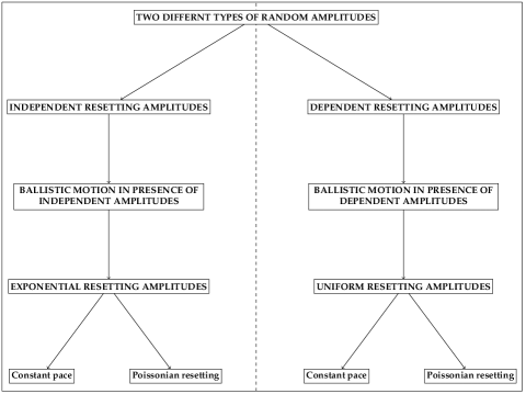
Figure 1: Flowchart of the two main concepts, independent and dependent random amplitude stochastic resetting (RASR) with specific choices of the resetting and propagation statistics.

We here develop the RASR model and discuss a range of applications going beyond the geophysical erosion picture drawn here. Examples include the dynamics of financial markets hit by occasional crises AGSR_1 ; AGSR_2 , population dynamics affected by partial extinction AGSR_3 , or germs affected by antibiotic treatment AGSR_4 . We note that we call RASR a resetting process despite the fact that the "reset" leads to a random position. However, the RASR process keeps the idea of classical resetting in that the propagation of the test particle is occasionally interrupted by a significant shift. In the search context mentioned above the RASR process thus represents a new class of intermittent search processes in which the searcher does not intermittently return to its "nest" but restarts its search at a range of key points (points of previous search success, etc.).

The layout of the paper is as follows (compare also the scheme in figure 1). We first develop the general resetting picutre of our RASR model in Section II. Section III introduces the concept of indepentent resetting, in which the coordinate of the process does not depent on the position before resetting. The opposite case, dependent resetting is developed in Section IV. In both cases we consider specific cases for the timing of the resets and the resetting amplitude statistic. We draw our Conclusions in Section V, some additional derivations are deferred to the Appendices.

II General resetting picture

In the RASR model $\psi(t)$ denotes the probability density function (PDF) of time spans between resetting events, and the PDF for the time $t$ at which the $n$th resetting event occurs is

$$\psi_{n}(t)=\int_{0}^{t}\psi_{n-1}\left(t-t^{\prime}\right)\psi(t^{\prime})dt^{\prime}$$ (1)

with $\psi_{0}(t)=\delta(t)$. In Laplace space, therefore, $\tilde{\psi}_{n}(s)=\tilde{\psi}^{n}(s)$. The probability

$$\Psi(t)=1-\int_{0}^{t}\psi(t^{\prime})dt^{\prime}$$ (2)

of no reset up to $t$ becomes $\tilde{\Psi}(s)=(1-\tilde{\psi}(s))/s$. Finally, the probability to have exactly $n$ resets up to $t$ is

$$\Phi_{n}(t)=\int_{0}^{t}\psi_{n}(t^{\prime})\Psi(t-t^{\prime})dt^{\prime}.$$ (3)

In what follows we consider independent, identically distributed (iid) resetting time intervals by using the examples of constant interval lengths ("constant pace") and Poisson-distributed intervals. The RASR process can have independent resetting amplitudes $z_{n}$ at the $n$th step that do not have a lower bound (Fig. 2a, b). For dependent (bounded) resetting amplitudes the process never crosses to negative heights $x(t_{n})$ (Fig. 2c, d).

Let the term $x(t)|x(t_{0})$ denote the position $x$ at a certain time $t$ provided that at time $t_{0}$ the position was $x_{0}=x(t_{0})$. For the derivations of the "first resetting picture" we will use the general relation

$$x(t)|x(t_{0})=\left\{\begin{array}[]{ll}y(t)|x(t_{0})&\mbox{with probability }\Psi(t-t_{0})\\ &\mbox{ for }t_{0}\leq t,\\[9.10509pt] x(t)|x(t_{1})&\mbox{with probability}\\ &\int\limits_{t_{0}}^{t}dt_{1}\psi(t_{1}-t_{0})\end{array}\right.\$$ (8)

Eq. (8) shows two possibilities. The upper line describes the possibility of no reset in $[t_{0},t]$ with the corresponding probability $\Psi(t-t_{0})$. In this scenario the process, starting at position $x_{0}=x(t_{0})$ at time $t_{0}$, fulfils a specific displacement process $y(t)$. Thus, with probability $\Psi(t-t_{0})$ the process $x(t)=y(t)$, which is stochastically described by $G(y,t;x_{0},t_{0})$. The lower line of Eq. (8) describes the first resetting point $x(t_{1})$ at the random resetting event $t_{1}$ as a new initial condition of $x(t)$. The new initial condition $x_{1}$ at $t_{1}$ will be described by the distribution $\phi(x_{1},t_{1};x_{0},t_{0})$, which is, without loss of generality, dependent on the previous initial condition $x_{0}$ at $t_{0}$. The corresponding probability for this event is $\int_{t_{0}}^{t}dt_{1}\psi(t_{1}-t_{0})$ for $t_{1}\in[t_{0},t]$.

With Eq. (8) we can find the expression for the corresponding PDF $P(x,t;x_{0},t_{0})$,

$$P(x,t;x_{0},t_{0}) = \Psi(t-t_{0})G(x,t;x_{0},t_{0})$$ (9)

$$+\int_{t_{0}}^{t}dt_{1}\psi(t_{1}-t_{0})\int_{-\infty}^{\infty}dx_{1}\phi_{1}(x_{1},t_{1};x_{0},t_{0})$$

$$\times P(x,t;x_{1},t_{1}).$$

In Eq. (9), $\phi_{1}(x_{1},t_{1};x_{0},t_{0})$ is the distribution of the first resetting point $x_{1}=x(t_{1})$ at time $t_{1}$ under the condition that the process started at position $x_{0}$ at time $t_{0}$. The computation of $\phi_{1}(x_{1},t_{1};x_{0},t_{0})$ depends on which kind of resetting mechanism we will use.

III Independent resetting picture

For independent resetting the height after the $n+1$st resetting event is

$$x(t_{n+1})=y(t_{n+1})|x(t_{n})+z_{n+1}$$ (10)

with the initial condition $x(t_{0})=x_{0}$. Here $y(t_{n+1})|x(t_{n})$ defines the unperturbed motion during the time interval $t_{n+1}-t_{n}$ starting from point $x(t_{n})$. Moreover, $z_{n+1}$ is an iid resetting amplitude of negative value, $z_{i}\in(-\infty,0)$. This setup corresponds to our picture of sudden massive erosion, population decimation, or financial market loss, in which the resetting amplitude is viewed independent of the process. Conceptually, this type of RASR corresponds to jump diffusion with one-sided jump lengths Kou ; porporato .

For $n=0$, Eq. (10) yields

$$x(t_{1})=y(t_{1})|x_{0}+z_{1}.$$ (11)

The sum of two random variables implies the convolution of the corresponding PDFs. Thus, with Eq. (11), $\phi_{1}(x_{1},t_{1};x_{0},t_{0})$ is

$$\phi_{1}(x_{1},t_{1};x_{0},t_{0})=\int_{-\infty}^{\infty}dyG(y,t_{1};x_{0},t_{0})q(x_{1}-y).$$ (12)

The PDF $P(x,t;x_{0},t_{0})$ to propagate from $x_{0}$ at $t_{0}$ to $x(t)$ is obtained by plugging relation (12) into Eq. (9), yielding

$$P(x,t;x_{0},t_{0}) = \Psi(t-t_{0})G(x,t;x_{0},t_{0})$$ (13)

$$+\int_{t_{0}}^{t}dt_{1}\psi(t_{1}-t_{0})\int_{-\infty}^{\infty}dyG(y,t_{1};x_{0},t_{0})$$

$$\times\int_{-\infty}^{\infty}dx_{1}q(x_{1}-y)P(x,t;x_{1},t_{1}).$$

The first term on the right involves the PDF $G(x,t;x_{0},t_{0})$ for undisturbed motion without resetting, where the probability $\Psi(t)$ denotes no resetting during the time from $t_{0}$ to $t$. The second term describes free propagation from $(x_{0},t_{0})$ to the first resetting point at $(x_{1},t_{1})$, at which a reset to $x_{1}$ occurs with the amplitude PDF $q(x_{1}-y)$. Then the process is propagated by $P(x,t;x_{1},t_{1})$. Eq. (13) can be iterated to include all resetting steps. From that derivation one can see that the PDF $P(x,t;x_{0},t_{0})$ is homogeneous, $P(x,t;x_{0},t_{0})=P(x-x_{0},t-t_{0};0,0)$, exactly when $G$ is homogeneous. In the setting of Eq. (13) we can describe a general resetting process with arbitrary propagation and independent resetting events. The first resetting picture described here can be shown to be identical to the "last resetting picture", as demonstrated for independent resetting in Apps. A and B. We now consider special cases for the propagation, resetting times, and amplitudes.

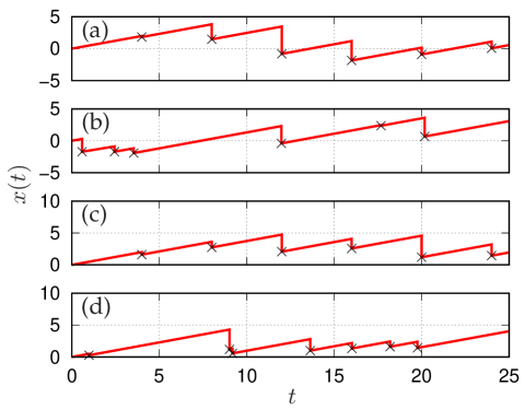
Figure 2: RASR sample paths with ballistic displacement ($v=0.5$) and independent (Poissonian with mean $\zeta=1.6$, panels (a) and (b)) as well as dependent (uniformly distributed, panels (c) and (d)) resetting amplitudes. In (a) and (c) resetting events ($\times$) occur at constant pace, in (b) and (d) with Poissonian waiting times, both with mean rate $r=1/4$.

III.1 Ballistic propagation

An illustrative example is given by ballistic propagation (and in fact a special case of the jump process considered in porporato ) with speed $v$, $G(x,t)=\delta(x-vt)$, where we set $x_{0}=0$ and $t_{0}=0$. To compute the characteristic function ${\hat{P}}(k,t)=\int_{-\infty}^{\infty}dx\exp(ikx)P(x,t)$ of $P(x,t)=P(x,t;x_{0}=0,t_{0}=0)$ for the first resetting picture (9) respectively the last resetting picture (96) in presence of a ballistic propagation, we use Eq. (9) with $G(x,t;y,\tau)=\delta\left(x-y-v\left(t-\tau\right)\right)$. The Laplace transform $\tilde{\hat{P}}(k,s)=\int_{0}^{\infty}dt\exp(-st){\hat{P}}(k,t)$ of the characteristic function ${\hat{P}}(k,t)$ then reads

$$P\left(x,t\right) = \Psi(t)\delta(x-vt)+\int\limits_{0}^{t}dt_{1}\psi(t_{1})\int\limits_{-\infty}^{\infty}dy\delta(y-vt_{1})$$

$$\times\int\limits_{-\infty}^{\infty}dx_{1}q(x_{1}-y)P(x-x_{1},t-t_{1}),$$

from which we obtain the Fourier transform

$${\hat{P}}(k,t) = \Psi(t)\exp(ikvt)$$ (14)

$$+\int\limits_{0}^{t}dt_{1}\psi(t_{1})\exp(ikvt_{1})\hat{q}(k)\hat{P}(k,t-t_{1}).$$

Finally, after an additional Laplace transform,

$$\tilde{{\hat{P}}}(k,s)=\tilde{\Psi}(s-ikv)+\tilde{\psi}(s-ikv)\hat{q}(k)\tilde{\hat{P}}(k,s),\\$$ (15)

we obtain the algebraic relation

$$\tilde{{\hat{P}}}(k,s)=\frac{\tilde{\Psi}(s-ikv)}{1-\tilde{\psi}(s-ikv)\hat{q}(k)}.$$ (16)

Eq. (16) is similar to the Montroll-Weiss equation montroll for continuous time random walk processes. Rewriting Eq. (16) in terms of a geometric series, $\tilde{\hat{P}}(k,s)$ becomes

$$\tilde{{\hat{P}}}(k,s)=\tilde{\Psi}(s-ikv)\sum_{n=0}^{\infty}\left(\tilde{\psi}(s-ikv)\hat{q}(k)\right)^{n}.$$ (17)

With definition (3) we end up with the compact expression

$$\tilde{{\hat{P}}}(k,s)=\sum_{n=0}^{\infty}\tilde{\Phi}_{n}(s-ikv)\hat{q}^{n}(k).$$ (18)

Note that by definition $\Phi_{n}(t)$ is the probability of exactly $n$ resetting events in $[0,t]$, and with $\int_{0}^{t}\psi_{n-1}\left(t-t^{\prime}\right)\psi(t^{\prime})dt^{\prime}$ ($\psi_{0}(t)=\delta(t)$, i.e., $\Phi_{0}(t)=\Psi(t)$), the Laplace transform of $\Phi_{n}(t)$ becomes $\tilde{\Phi}_{n}(s)=\tilde{\Psi}(s)\tilde{\psi}^{n}(s)$. With these relations we can perform the inverse Laplace transform of $\tilde{{\hat{P}}}(k,s)$ yielding the characteristic function ${\hat{P}}(k,t)$

$$\hat{P}(k,t)=\sum^{\infty}_{n=0}\Phi_{n}(t)\exp(ikvt)\hat{q}^{n}(k).$$ (19)

An alternative approach to derive the characteristic function is to use its representation as a jump diffusion process Kou ,

$$x(t)=vt+\sum^{n(t)}_{j=1}z_{j},$$ (20)

where the stochastic variable $n(t)$ is the number of resets in the interval $[0,t]$. The characteristic function can be computed as

$$\hat{P}(k,t) = \langle\exp(ikx(t))\rangle$$ (21)

$$= \exp(ikvt)\left<\prod^{n(t)}_{j=1}\exp(ikz_{j})\right>$$

$$= \sum^{\infty}_{n=0}\Phi_{n}(t)\exp(ikvt)\prod^{n}_{j=1}\langle\exp(ikz_{j})\rangle.$$

As $n(t)$ in this expression is a stochastic variable we need to sum up the probabilities $\Phi_{n}(t)$ of every possible value of $n\in\mathbb{N}$. Furthermore, we use the property of the $z_{j}$ to be iid random variables, along with the identity $\Phi_{0}(t)=\Psi(t)$. This leads us directly to Eq. (19).

Define now $q_{n}(z)$ as the distribution of the total jump size $z$ after $n$ iid jumps with distribution $q(z)$. The relation between $q_{n}(z)$ and $q(z)$ is then

$$q_{n}(z)=\left\{\begin{array}[]{ll}\int\limits_{-\infty}^{\infty}dz^{\prime}q_{n-1}(z-z^{\prime})q(z^{\prime})&n\geq 1\\ \delta(z)&n=0\end{array}\right.,$$ (22)

and thus

$${\hat{q}}_{n}(k)={\hat{q}}^{n}(k).$$ (23)

With $q_{n}(z)$ from Eq. (23) we take the inverse Fourier transform of the characteristic function $\hat{P}(k,t)$, Eq. (19). Thus, $P(x,t)$ takes on the form

$$P(x,t) = \sum^{\infty}_{n=0}\Phi_{n}(t)q_{n}(x-vt),$$ (24)

$$= \Psi(t)\delta(x-vt)+\sum^{\infty}_{n=1}\Phi_{n}(t){q}_{n}(x-vt)$$

Calculation of moments

For the average $\langle x(t)\rangle$ and the variance $\mathrm{Var}\{x(t)\}$ of the variable $x(t)$ we compute the first and second derivatives of $\hat{P}(k,t)$, Eq. (19),

$$\hat{P}^{\prime}(k,t) = \sum^{\infty}_{n=0}\Phi_{n}(t)\exp(ikvt)\hat{q}^{n}(k)\left(ivt+\frac{n\hat{q}^{\prime}(k)}{\hat{q}(k)}\right),$$

$$\hat{P}^{\prime\prime}(k,t) = \sum^{\infty}_{n=0}\Phi_{n}(t)\exp(ikvt)\hat{q}^{n}(k)$$ (25)

$$\times\left(\left(ivt+\frac{n\hat{q}^{\prime}(k)}{\hat{q}(k)}\right)^{2}+n\frac{\hat{q}^{\prime\prime}(k)\hat{q}(k)-\left(\hat{q}^{\prime}(k)\right)^{2}}{\left(\hat{q}(k)\right)^{2}}\right).$$

Let $\langle z\rangle=-i\hat{q}^{\prime}(0)$ be the average of the random independent amplitude $z$ with the corresponding distribution $q(z)$. Then with Eq. (III.1) the average $\langle x(t)\rangle$ of $x(t)$ is

$$\langle x(t)\rangle=-i\hat{P}^{\prime}(0,t)=\sum^{\infty}_{n=0}\Phi_{n}(t)\big{(}vt+n\langle z\rangle\big{)}.$$ (26)

Now let $\mathrm{Var}\{z\}=\left(\hat{q}^{\prime}(0)\right)^{2}-\hat{q}^{\prime\prime}(0)$ be the variance of the random independent amplitude $z$ with distribution $q(z)$. Thus, the variance $\mathrm{Var}\{x(t)\}$ of the position $x(t)$ becomes

$$\mathrm{Var}\{x(t)\} = \left(\hat{P}^{\prime}(0,t)\right)^{2}-\hat{P}^{\prime\prime}(0,t),$$ (27)

$$=\sum^{\infty}_{n=0}\Phi_{n}(t)\big{(}(vt+n\langle z\rangle)^{2}+n\mathrm{Var}\{z\}\big{)}-\langle x(t)\rangle^{2}.$$

III.2 Ballistic propagation with exponential resetting amplitudes

For the concrete choice of exponential resetting amplitudes, defined by

$$q(z)=\Theta(-z)\zeta^{-1}\exp\left(\frac{z}{/\zeta}\right),$$ (28)

the distribution $q_{n}(z)$ becomes

$$q_{n}(z) = \frac{1}{2\pi}\int_{-\infty}^{\infty}dk\exp(-ikz)\left(\frac{1}{1+ik\zeta}\right)^{n},$$

$$= \frac{(-z)^{n-1}}{\zeta^{n}(n-1)!}\exp\left(\frac{z}{\zeta}\right)\Theta(-z).$$

The density $P(x,t)$ (Eq. (24)) then yielsd in the form

$$P(x,t) = \Psi(t)\delta(x-vt)+\sum^{\infty}_{n=1}\Phi_{n}(t)\frac{(vt-x)^{n-1}}{\zeta^{n}(n-1)!}$$ (29)

$$\times\exp\left(\frac{x-vt}{\zeta}\right)\Theta(vt-x).$$

The Fourier transform of $q(z)$ is $\hat{q}(k)=1/(1+ik\zeta)$. With the first and second derivative of $\hat{q}(k)$,

$$\hat{q}^{\prime}(k)=\frac{-i\zeta}{(1+ik\zeta)^{2}},\quad\hat{q}^{\prime\prime}(k)=\frac{-2\zeta^{2}}{(1+ik\zeta)^{3}}$$ (30)

we get the average and the variance of $z$,

$$\langle z\rangle = -i\hat{q}^{\prime}(0)=-\zeta$$

$$\mathrm{Var}\{z\} = \left(\hat{q}^{\prime}(0)\right)^{2}-\hat{q}^{\prime\prime}(0)=-\zeta^{2}+2\zeta^{2}=\zeta^{2}.$$ (31)

The mean $\langle x(t)\rangle$ (Eq. (26)) now becomes

$$\langle x(t)\rangle=\sum^{\infty}_{n=0}\Phi_{n}(t)\times(vt-n\zeta),$$ (32)

and the variance $\mathrm{Var}\{x(t)\}$ (Eq. (27)) reads

$$\mathrm{Var}\{x(t)\} = \sum^{\infty}_{n=0}\Phi_{n}(t)\times\left((vt-n\zeta)^{2}+n\zeta^{2}\right)$$ (33)

$$-\left(\sum^{\infty}_{n=0}\Phi_{n}(t)\times(vt-n\zeta)\right)^{2}.$$

Ballistic propagation with exponential resetting amplitude and Poissonian resetting times

As a specific example we consider the combination of an exponential resetting amplitude PDF (28) of width $\zeta$ and Poissonian resetting times with distribution

$$\psi(t)=r\exp(-rt).$$ (34)

This implies the distributions

$$\tilde{\psi}(s)=\frac{r}{r+s},\,\,\,\tilde{\Psi}(s)=\frac{1-{\tilde{\psi}}(s)}{s}=\frac{1}{r+s},$$ (35)

and from this expression we find the Laplace transform

$$\tilde{\Phi}_{n}(s)=\tilde{\Psi}(s)\tilde{\psi}^{n}(s)=\frac{1}{r}\left(\frac{r}{r+s}\right)^{n+1}.$$ (36)

After Laplace inversion,

$$\Phi_{n}(t)=\frac{(rt)^{n}}{n!}\exp(-rt).$$ (37)

This yields the density $P(x,t)$ (Eq. (29)) for this case,

$$P(x,t) = \exp(-rt)\delta(x-vt)+\sum^{\infty}_{n=1}\frac{(rt)^{n}(vt-x)^{n-1}}{\zeta^{n}n!(n-1)!}$$ (38)

$$\times\exp\left(\frac{x-vt-rt\zeta}{\zeta}\right)\Theta(vt-x).$$

With the representation

$$I_{1}(\xi)=\frac{\xi}{2}\sum^{\infty}_{n=0}\frac{\left(\xi^{2}/4\right)^{n}}{n!(n+1)!}$$ (39)

of the modified Bessel function of the first kind we then obtain our result,

$$P(x,t) = e^{-rt}\delta(x-vt)+\exp([x-vt-rt\zeta]/\zeta)$$ (40)

$$\times\sqrt{\frac{rt/\zeta}{vt-x}}I_{1}\left(2\sqrt{\frac{rt}{\zeta}(vt-x)}\right)\Theta(vt-x).$$

The mean $\langle x(t)\rangle$ of $x(t)$ (Eq. (32)) is

$$\langle x(t)\rangle = \sum^{\infty}_{n=0}\frac{(rt)^{n}}{n!}\exp(-rt)\times(vt-n\zeta),$$ (41)

$$= (v-r\zeta)t.$$

The mean position thus depends linearly on $t$ and increases or decreases, depending on the sign of $(v-r\zeta)$. The variance $\mathrm{Var}\{x(t)\}$ (Eq. (33)) has the form

$$\mathrm{Var}\{x(t)\} = \sum^{\infty}_{n=0}\frac{(rt)^{n}}{n!}\exp(-rt)\times\left((vt-n\zeta)^{2}+n\zeta^{2}\right)$$ (42)

$$-(vt-rt\zeta)^{2},$$

$$= 2rt\zeta^{2}.$$

The variance is thus also proportional to $t$, but it is $v$-independent.

Fig. 3 shows $P(x,t)$ at different times: the maximum value decreases and the PDF gradually shifts away from negative values. The possibility of no reset up to time $t$ is encoded in the finite value at $x=vt$, the inset shows a discontinuity of $P(x,t)$ at $x=vt$ and the exponential relation between the probability of no reset and time $t$.

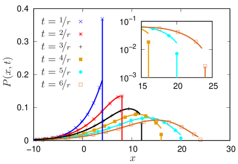
Figure 3: Height profile PDF $P(x,t)$ as function of $x$ for six different $t$ for ballistic motion with Poissonian resetting times and exponential resetting amplitudes. The probability of no reset until $t$ is represented by the vertical line at $x=vt$, it is shown on log-lin scale for different $t$ in the inset. Simulations results are shown by points, the analytical results are shown by solid lines. Parameters: $v=0.5$, $r=0.125$, and $\zeta=2$.

In App. C we derive the Fourier transform of the PDF $P(x,t)$ from the master equation formulation for the case of ballistic propagation, Poissonian resetting times and arbitrary independent resetting amplitudes. The result (119) then corresponds to Eq. (19) with the choice (37) for $\Phi_{n}(t)$.

III.3 Ballistic displacement with constant pace and exponential resetting amplitudes

We now consider another variant of ballistic propagation, namely, of a constant duration between successive resetting events, which we refer to as constant pace. The distribution of the resetting interval lengths is

$$\psi(t)=\delta\left(t-\frac{1}{r}\right).$$ (43)

In Laplace space this implies the distributions

$$\tilde{\psi}(s)=\exp\left(-\frac{s}{r}\right),\,\,\,\tilde{\Psi}(s)=\frac{1-\exp(-s/r)}{s},\\$$ (44)

and consequently

$$\tilde{\Phi}_{n}(s)=\frac{\exp(-ns/r)-\exp(-(n+1)s/r)}{s},$$ (45)

After Laplace inversion,

$$\Phi_{n}(t)=\Theta\left(t-\frac{n}{r}\right)-\Theta\left(t-\frac{n+1}{r}\right).$$ (46)

Thus, the density $P(x,t)$ (Eq. (29)) is given by

$$P(x,t) = \left(\Theta(t)-\Theta\left(t-\frac{1}{r}\right)\right)\delta(x-vt)$$ (47)

$$+\Theta(vt-x)\sum^{\infty}_{n=1}\frac{(vt-x)^{n-1}}{\zeta^{n}(n-1)!}\exp\left(\frac{x-vt}{\zeta}\right)$$

$$\times\left(\Theta\left(t-\frac{n}{r}\right)-\Theta\left(t-\frac{n+1}{r}\right)\right).$$

The mean $\langle x(t)\rangle$ of $x(t)$ (Eq. (32)) becomes

$$\langle x(t)\rangle = \sum^{\infty}_{n=0}\left(\Theta\left(t-\frac{n}{r}\right)-\Theta\left(t-\frac{n+1}{r}\right)\right)$$ (48)

$$\times(vt-n\zeta)$$

$$= vt-\zeta\lfloor rt\rfloor,$$

where we introduce the floor function $\lfloor x\rfloor=\max\{l\in\mathbb{Z}|l\leq x\}$. The variance $\mathrm{Var}\{x(t)\}$ (Eq. (33)) reads

$$\mathrm{Var}\{x(t)\} = \zeta^{2}\sum^{\infty}_{n=0}\left(\Theta\left(t-\frac{n}{r}\right)-\Theta\left(t-\frac{n+1}{r}\right)\right)n,$$ (49)

$$= \zeta^{2}\lfloor rt\rfloor.$$

In the long time limit results (48) and (49) coincide with the corresponding mean and variance in the Poissonian resetting time scenario, Eqs. (41) and (42).

In Fig. 4 the mean position and variance are shown for two different examples of ballistic propagation and exponential resetting amplitudes, demonstrating the linear growth of the mean height. In this example we see that the constant pace scenario has the same mean as the Poissonian resetting model but half the variance, as can also be seen from comparison of Eqs. (42) and (49).

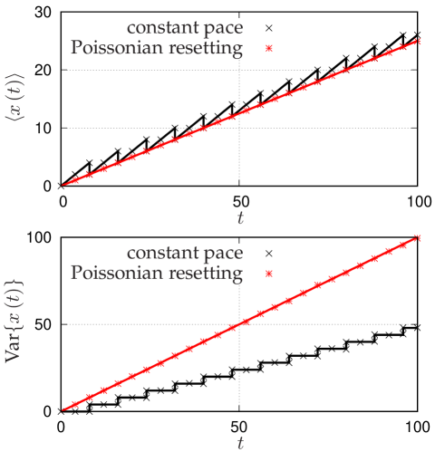
Figure 4: Average and variance of the height $x$ as function for $t$ for exponential resetting amplitudes and ballistic motion, with Poissonian and constant pace resetting times. Points represent simulations results, solid lines are the analytical results. Parameters: $v=0.5$, $r=0.125$, and $\zeta=2$.

Let us compare the difference between the cases of constant pace and Poissonian resetting intervals in more detail. Fig. 5 illustrates the PDF $P(x,t)$ for constant pace (left panel) and Poissonian resetting (right panel) at different times. For the chosen values the maximum of the PDF increases with time, and the standard deviation of the PDF increases in both panels. In the case of constant pace resetting, we showed the distribution immediately after resetting in Fig. 5. For Poissonian resetting the possibility that no reset occurs up to time $t$ is encoded in the finite value at $x=vt$. Its value is detailed in the inset, showing a discontinuity of $P(x,t)$ at $x=vt$ and the exponential relation between the probability of no reset and time $t$.

Fig. 6 shows the behavior of the average (left panel) and variance (right panel) of $x(t)$. For constant pace resetting the average $\langle x(t)\rangle$ increases linearly in time between successive resetting events, however the variance of $x(t)$ does not change in this time span. The corresponding PDF moves linearly in time, but does not change its shape during these time spans. The shape of the distribution only change at the resetting events. As it can be seen in Fig. 6 the variance $\mathrm{Var}\{x(t)\}$ only increases at these times. For Poissonian resetting the mean position depends linearly on $t$ and increases or decreases, depending on the sign of $(v-r\zeta)$. Both possibilities are shown in Fig. 6. Moreover, in presence of constant pace resetting, we can see that $\langle x(t)\rangle$ increases faster than for Poissonian resetting during the resetting interval lengths. However, under the same choice of parameter the mean for constant pace resetting coincides with the Poissonian resetting at the resetting events. For Poissonian resetting the relation between $\mathrm{Var}\{x(t)\}$ and $t$ is linear and increases faster as for "constant pace" resetting.

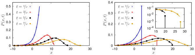
Figure 5: Height profile $P(x,t)$ as function of $x$ for four different $t$, for ballistic motion with exponential resetting amplitudes and two different resetting scenarios. Left: "constant pace" resetting. Right: Poissonian resetting. The probability of no reset until $t$ is represented by the vertical line at $x=vt$, it is shown on log-lin scale for different $t$ in the inset of the right panel. Points: simulations, Solid lines: analytical results. Parameters: $v=0.5$, $r=0.125$, and $\zeta=2$.

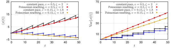
Figure 6: Average and variance of the height $x$ as function of time $t$ for exponential resetting amplitudes and ballistic motion, with Poissonian and "constant pace" resetting. Points represent simulations, solid lines the analytical results. For all realizations, $r=0.125$.

IV Dependent resetting picture

In many realistic situations the height $x(t)$ cannot assume negative values, e.g., when the deposits in a river bed shrink until they reach a solid bedrock, when the value of a given stock becomes zero, or when a population goes extinct. Random-amplitude resetting processes with strictly positive $x$ in our framework are described by dependent resetting amplitudes, the main novel feature introduced in this work.

For such dependent resetting amplitudes we use the following relation between consecutive resetting points,

$$\left\{\begin{array}[]{ll}x(t_{n+1})=(y(t_{n+1})|x(t_{n}))\times c_{n+1}\\ x(t_{0})=x_{0}\end{array}\right.,$$ (52)

where the $c_{n}\in[0,1)$ are iid random variables of the running index $n$. For $n=0$, Eq. (52) yields

$$x(t_{1})=(y(t_{1})|x_{0})\times c_{1}.$$ (53)

With Eq. (53), $\phi_{1}(x_{1},t_{1};x_{0},t_{0})$ becomes

$$\phi_{1}(x_{1},t_{1};x_{0},t_{0})=\int_{0}^{\infty}\frac{dy}{y}G(y,t_{1};x_{0},t_{0})f_{C}\left(\frac{x_{1}}{y}\right).$$ (54)

In Eq. (54) we only allow movement for positive heights, $0\leq y<\infty$. Due to our requirement that height $x(t)$ cannot assume negative values, we impose the additional condition that $f_{C}(c_{n})=0$ for $c_{n}<0$ and $c_{n}\geq 1$, such that we only have to consider the range $0\leq c_{1}=x_{1}/y<1$, in which $f_{C}(c_{1})\neq 0$. Thus we have the inequality $0\leq x_{1}/y<1$, or

$$0\leq x_{1}<y.$$ (55)

For dependent resetting amplitudes we get the first resetting picture of the process if we substitute $\phi_{1}(x_{1},t_{1};x_{0},t_{0})$, Eq. (54), into Eq. (9) and considering the range of $x_{1}$ for which $f_{C}(x_{1}/y)\neq 0$ (compare Eq. (55)). Thus, we get

$$P(x,t;x_{0},t_{0}) = \Psi(t-t_{0})G(x,t;x_{0},t_{0})$$ (56)

$$+\int_{t_{0}}^{t}dt_{1}\psi(t_{1}-t_{0})\int_{0}^{\infty}\frac{dy}{y}G(y,t_{1};x_{0},t_{0})$$

$$\times\int_{0}^{y}dx_{1}f_{C}(x_{1}/y)P(x,t;x_{1},t_{1}).$$

The key difference to Eq. (13) is that the $y$-integration is restricted to $y\in[0,\infty)$ and that the resetting length PDF $q(x_{1}-y)$ is replaced by the scaling function $y^{-1}f_{C}(x_{1}/y)$, that in turn is part of the product distribution (54). We derive the last resetting picture corresponding to the first resetting picture (56) in App. D. We note that when the PDF $G$ is homogenous in space and time, the PDF $P$ is still homogeneous in time but the spatial homogeneity is lost (App. D).

IV.1 Reduction to classical stochastic resetting

Before proceeding with our analysis we stop to proof that our RASR process with dependent resetting amplitudes is a generalization of classical SR. In fact we can prove this equivalence for both the first resetting picture and the last resetting picture if we set $f_{C}(c_{n})=\delta(c_{n})$ and use Poissonian resetting $\psi(t)=r\exp(-rt)$ along with the initial position $x_{0}=0$. With this deterministic resetting mechanism we can verify the results of RIL_3 for the first renewal picture and Evans2 for the last renewal picture of SR.

In the first resetting picture we have in our framework

$$P(x,t;0,0) = \exp(-rt)G(x,t;0,0)+\int\limits_{0}^{t}dt_{1}r\exp(-rt_{1})$$

$$\times\int\limits_{0}^{\infty}\frac{dy}{y}G(y,t_{1};0,0)\int\limits_{0}^{y}dx_{1}\delta\left(\frac{x_{1}}{y}\right)P(x,t;x_{1},t_{1})$$

$$=\exp(-rt)G(x,t;0,0)+r\int\limits_{0}^{t}dt_{1}\exp(-rt_{1})$$

$$\int\limits_{0}^{\infty}dyG(y,t_{1};0,0)\int\limits_{0}^{1}dc_{1}\delta(c_{1})P(x,t;c_{1}y,t_{1}),$$

in which $c_{1}=x_{1}/y$. This implies that

$$P(x,t;0,0) = \exp(-rt)G(x,t;0,0)+r\int\limits_{0}^{t}dt_{1}\exp(-rt_{1})$$ (57)

$$\times\int\limits_{0}^{\infty}dyG(y,t_{1};0,0)P(x,t;0,t_{1})$$

$$= \exp(-rt)G(x,t;0,0)+r\int\limits_{0}^{t}dt_{1}\exp(-rt_{1})$$

$$\times P(x,t;0,t_{1}),$$

and therefore proves the equivalence to RIL_3 with $x_{0}=0$.

Conversely, in the last resetting picture we have [cf. Eq. (134)]

$$P(x,t;0,0) = \exp(-rt)G(x,t;0,0)+\sum^{\infty}_{n=1}\int\limits_{0}^{t}d\tau_{n}\int\limits_{0}^{1}dc_{n}\int\limits_{0}^{\infty}dy^{\prime}_{n}\left(\prod^{n-1}_{i=1}\int\limits_{0}^{\tau_{n+1-i}}d\tau_{n-i}r\exp(-r(\tau_{n+1-i}-\tau_{n-i}))\right)$$ (58)

$$\times\left(\prod^{n-1}_{i=1}\int\limits_{0}^{\infty}dy^{\prime}_{n-i}G(y^{\prime}_{n+1-i},\tau_{n+1-i};c_{n-i}y^{\prime}_{n-i},\tau_{n-i})\int\limits_{0}^{1}dc_{n-i}\delta(c_{n+1-i})\right)$$

$$\times\delta(c_{1})r\exp(-r\tau_{1})G(y^{\prime}_{1},\tau_{1};0,0)\exp(-r(t-\tau_{n}))G(x,t;c_{n}y^{\prime}_{n},\tau_{n})$$

$$= \exp(-rt)G(x,t;0,0)+\sum^{\infty}_{n=1}r^{n}\int\limits_{0}^{t}d\tau_{n}\left(\prod^{n-1}_{i=1}\int\limits_{0}^{\tau_{n+1-i}}d\tau_{n-i}\right)\exp(-r[\tau_{n}-\tau_{n-1}])\exp(-r[\tau_{n-1}-\tau_{n-2}])$$

$$\times\ldots\times\exp(-r[\tau_{3}-\tau_{2}])\exp(-r[\tau_{2}-\tau_{1}])\exp(-r\tau_{1})\exp(-r[t-\tau_{n}])G(x,t;0,\tau_{n})$$

$$= \exp(-rt)G(x,t;0,0)+r\int\limits_{0}^{t}d\tau\sum^{\infty}_{n=1}\frac{(r\tau)^{n-1}}{(n-1)!}\exp(-rt)G(x,t;0,\tau),$$

with $\tau=\tau_{n}$. This demonstrates that

$$P(x,t;0,0)=\exp(-rt)G(x,t;0,0)+r\int\limits_{0}^{t}d\tau\exp(-r[t-\tau])G(x,t;0,\tau),$$ (59)

and completes our proof of equivalence with the formulation in Evans2 for $x_{0}=0$.

IV.2 Ballistic propagation with dependent resetting amplitude

For the spatial Laplace transform $\bar{P}(u,t;x_{0})=\int_{0}^{\infty}dx\exp(-ux)P(x,t;x_{0})$ of the one-sided density $P(x,t;x_{0})=P(x,t;x_{0},t_{0}=0)$ in the first resetting picture (56) respectively the last resetting picture (121) for the case of ballistic propagation, we use Eq. (121) with $G(x,t;y,\tau)=\delta(x-y-v(t-\tau))$. Collecting terms, $P(x,t;x_{0})$ reads

$$P(x,t;x_{0}) = \Psi(t)\delta(x-x_{0}-vt)+\sum^{\infty}_{n=1}\int\limits_{0}^{t}d\tau_{n}\int\limits_{0}^{1}dc_{n}\int\limits_{0}^{\infty}dy_{n}\times\left(\prod^{n-1}_{i=1}\int\limits_{0}^{\tau_{n+1-i}}d\tau_{n-i}\psi(\tau_{n+1-i}-\tau_{n-i})\right.$$ (60)

$$\left.\times\int\limits_{0}^{\infty}dy_{n-i}\delta(y_{n+1-i}-c_{n-i}y_{n-i}-v(\tau_{n+1-i}-\tau_{n-i}))\int\limits_{0}^{1}dc_{n-i}f_{C}(c_{n+1-i})\right)$$

$$\times f_{C}(c_{1})\psi(\tau_{1})\delta(y_{1}-x_{0}-v\tau_{1})\Psi(t-\tau_{n})\delta(x-c_{n}y_{n}-v(t-\tau_{n})),$$

and after the spatial Laplace transform we find

$$\bar{P}(u,t;x_{0}) = \Psi(t)\exp(-u(x_{0}+vt))+\sum^{\infty}_{n=1}\int\limits_{0}^{t}d\tau_{n}\int\limits_{0}^{1}dc_{n}\left(\prod^{n-1}_{i=1}\int\limits_{0}^{\tau_{n+1-i}}d\tau_{n-i}\psi(\tau_{n+1-i}-\tau_{n-i})\int\limits_{0}^{1}dc_{n-i}f_{C}(c_{n+1-i})\right)$$ (61)

$$\times f_{C}(c_{1})\psi(\tau_{1})\Psi(t-\tau_{n})\exp\left(-u\left(x_{0}\prod^{n}_{j=0}c_{j}+v(t-\tau_{n})+v\sum^{n}_{j=1}(\tau_{j}-\tau_{j-1})\prod^{n}_{k=j}c_{k}\right)\right),$$

in which $c_{0}=1$ and $\tau_{0}=0$. Performing a Laplace transform in time (with the corresponding Laplace variable $s$), in addition, our general result for the PDF reads

$$\tilde{\bar{P}}(u,s;x_{0}) = \sum^{\infty}_{n=0}\tilde{\Psi}(s+uv)\left(\prod^{n}_{k=1}\int\limits_{0}^{1}dc_{k}f_{C}(c_{k})\tilde{\psi}\left(s+uv\prod^{k}_{i=1}c_{i}\right)\right)\exp\left(-ux_{0}\prod^{n}_{j=0}c_{j}\right).$$ (62)

To compute the mean

$$\langle x(t)|x_{0}\rangle=-{\bar{P}}^{\prime}(0,t;x_{0})$$ (63)

and variance

$$\mathrm{Var}\{x(t)|x_{0}\}={\bar{P}}^{\prime\prime}(0,t;x_{0})-\left({\bar{P}}^{\prime}(0,t;x_{0})\right),$$ (64)

we use the first and second derivatives of $\bar{P}(u,t;x_{0})$, Eq. (61), with respect to $u$ and set $u=0$. It is easier to work with the Laplace transform (62) in time. General formulas for the first and second derivatives of Eq. (62) with respect to the Laplace variable $u$ are presented in App. E. They will be used in Sections IV.3 and IV.4 below.

IV.3 Ballistic displacement with arbitrary resetting times and uniform dependent resetting amplitudes

We now turn to the ballistic displacement process with arbitrary resetting intervals but the specific choice of uniform dependent resetting amplitudes. This choice allows us to specify (136) and (138) when we inlude $f_{C}(c)=1$. Thus for the first and second moment of $c$ we get $\langle c\rangle=1/2$ and $\langle c^{2}\rangle=1/3$. The first derivative $\tilde{\bar{P}}^{\prime}(u,t;x_{0})$ becomes

$$\tilde{\bar{P}}^{\prime}(0,s;x_{0})=\sum^{\infty}_{n=0}\left(v\left(\tilde{\psi}^{n}(s)\tilde{\Psi}^{\prime}(s)+\tilde{\psi}^{n-1}(s)\tilde{\psi}^{\prime}(s)\tilde{\Psi}(s)\left(1-\frac{1}{2^{n}}\right)\right)-x_{0}\left(\frac{\tilde{\psi}(s)}{2}\right)^{n}\tilde{\Psi}(s)\right).$$ (65)

The second derivative $\tilde{\bar{P}}^{\prime\prime}(u,t;x_{0})$ reads

$$\tilde{\bar{P}}^{\prime\prime}(0,s;x_{0}) = \sum^{\infty}_{n=0}v^{2}\left(\tilde{\psi}^{n}(s)\tilde{\Psi}^{\prime\prime}(s)+\frac{1}{2}\tilde{\psi}^{n-1}(s)\tilde{\psi}^{\prime\prime}(s)\tilde{\Psi}(s)\left(1-\frac{1}{3^{n}}\right)+2\tilde{\psi}^{n-1}(s)\tilde{\psi}^{\prime}(s)\tilde{\Psi}^{\prime}(s)\left(1-\frac{1}{2^{n}}\right)\right)$$ (66)

$$+\sum^{\infty}_{n=0}\left(v^{2}\tilde{\Psi}(s)\tilde{\psi}^{\prime 2}(s)\tilde{\psi}^{n-2}(s)\left(1+\frac{3}{3^{n}}-\frac{4}{2^{n}}\right)+x^{2}_{0}\left(\frac{\tilde{\psi}(s)}{3}\right)^{n}\tilde{\Psi}(s)\right)$$

$$-\sum^{\infty}_{n=0}2vx_{0}\left(\left(\frac{\tilde{\psi}(s)}{2}\right)^{n}\tilde{\Psi}^{\prime}(s)+2\tilde{\psi}^{n-1}(s)\tilde{\psi}^{\prime}(s)\tilde{\Psi}(s)\left(\frac{1}{2^{n}}-\frac{1}{3^{n}}\right)\right).$$

For constant pace resetting times, we have a periodic reset with $\psi(t)=\delta\left(t-1/r\right)$ corresponding to expressions (44). Thus, the resetting amplitude is the only stochastic variable in this process. After some algebra and Laplce inversion we find

$$\bar{P}^{\prime}(0,t;x_{0})=-\sum_{n=0}^{\infty}\Phi_{n}(t)\left(v\left(t-\frac{n}{r}\right)+\frac{v}{r}\left(1-\frac{1}{2^{n}}\right)+\frac{x_{0}}{2^{n}}\right),$$ (67)

in which $\Phi_{n}(t)=\Theta\left(t-n/r\right)-\Theta\left(t-(n+1)/r\right)$. The mean $\langle x(t)|x_{0}\rangle$, Eq. (63), then yields in the form

$$\langle x(t)|x_{0}\rangle=x_{0}+vt+\sum^{\lfloor rt\rfloor}_{n=1}\left(\frac{1}{2^{n}}\left(\frac{v}{r}-x_{0}\right)-\frac{v}{r}\right)$$ (68)

with the asymptotic properties

$$\limsup_{t\to\infty}\langle x(t)|x_{0}\rangle=2\frac{v}{r},$$

$$\liminf_{t\to\infty}\langle x(t)|x_{0}\rangle=\frac{v}{r}.$$ (69)

Thus, in the long time limit the oscillating average $\langle x(t)|x_{0}\rangle$ is restricted by the two bounds (69).

Similarly we compute the second derivative of the PDF,

$$\bar{P}^{\prime\prime}(0,t;x_{0}) = \sum_{n=0}^{\infty}\Phi_{n}(t)\left(v^{2}\left(t-\frac{n}{r}\right)^{2}+\frac{2v^{2}}{r}\left(t-\frac{n}{r}\right)\left(1-\frac{1}{2^{n}}\right)+\frac{v^{2}}{2r^{2}}\left(3+\frac{5}{3^{n}}-\frac{8}{2^{n}}\right)-\frac{2vx_{0}}{2^{n}}\left(t-\frac{n}{r}\right)\right)$$ (70)

$$+\sum_{n=0}^{\infty}\Phi_{n}(t)\left(\frac{4vx_{0}}{r}\left(\frac{1}{2^{n}}-\frac{1}{3^{n}}\right)+\frac{x_{0}^{2}}{3^{n}}\right),$$

in which $\Phi_{n}(t)=\Theta\left(t-n/r\right)-\Theta\left(t-(n+1)/r\right)$. The variance, Eq. (64), finally reads

$$\mathrm{Var}\{x(t)|x_{0}\} = \sum^{\lfloor rt\rfloor}_{n=1}\left(x^{2}_{0}\left(\frac{3}{4^{n}}-\frac{2}{3^{n}}\right)+2\frac{x_{0}v}{r}\left(\frac{4}{3^{n}}-\frac{3}{4^{n}}-\frac{1}{2^{n}}\right)+\frac{1}{2}\left(\frac{v}{r}\right)^{2}\left(\frac{6}{4^{n}}+\frac{4}{2^{n}}-\frac{10}{3^{n}}\right)\right)$$ (71)

$$\stackrel{{\scriptstyle t\to\infty}}{{\longrightarrow}} \frac{1}{2}\left(\frac{v}{r}\right)^{2}.$$

IV.4 Ballistic propagation and Poissonian resetting times

We now consider Poissonian resetting intervals with rate $r$, $\psi(t)=r\exp(-rt)$. Such exponential distributions are in fact used in several SR studies, including Evans1 ; RM_del3 ; RIL_5 ; SC_1 . For the resetting amplitudes we first derive a general solution and then consider specific examples.

We start from Eqs. (136) and (138) and use the resetting time distributions with their Laplace transforms $\tilde{\psi}(s)=r/(r+s)$ and $\tilde{\Psi}(s)=1/(r+s)$. Evaluating the geometric series we obtain the derivatives of the PDF. After Laplace inversion, these read

$$\bar{P}^{\prime}(0,t;x_{0}) = \frac{v}{r\left(1-\langle c\rangle\right)}\left(\exp\left(-rt\left(1-\langle c\rangle\right)\right)-1\right)-x_{0}\exp\left(-rt\left(1-\langle c\rangle\right)\right),$$ (72)

$$\bar{P}^{\prime\prime}(0,t;x_{0}) = \frac{2v^{2}}{r^{2}\left(\langle c\rangle-\langle c^{2}\rangle\right)}\left(\frac{\exp\left(-rt\left(1-\langle c^{2}\rangle\right)\right)}{1-\langle c^{2}\rangle}-\frac{\exp\left(-rt\left(1-\langle c\rangle\right)\right)}{1-\langle c\rangle}\right)$$ (73)

$$+\frac{2v^{2}}{r^{2}\left(1-\langle c\rangle\right)\left(1-\langle c^{2}\rangle\right)}+x^{2}_{0}\exp(-rt[1-\langle c^{2}\rangle])$$

$$+\frac{2x_{0}v}{r\left(\langle c\rangle-\langle c^{2}\rangle\right)}\left(\exp(-rt[1-\langle c\rangle])-\exp(-rt[1-\langle c^{2}\rangle])\right).$$

We then derive the mean and variance,

$$\langle x(t)|x_{0}\rangle = \frac{v}{r\left(1-\langle c\rangle\right)}\left(1-\exp(-rt[1-\langle c\rangle])\right)+x_{0}\exp(-rt[1-\langle c\rangle]),$$ (74)

$$\mathrm{Var}\{x(t)|x_{0}\} = \frac{2v^{2}\exp(-rt)}{r^{2}(\langle c\rangle-\langle c^{2}\rangle)}\left(\frac{\exp(rt\langle c^{2}\rangle)}{1-\langle c^{2}\rangle}-\frac{\exp(rt\langle c\rangle)}{1-\langle c\rangle}\right)$$ (75)

$$+\frac{2v^{2}}{r^{2}\left(1-\langle c\rangle\right)}\left(\frac{1}{1-\langle c^{2}\rangle}+\frac{\exp(-rt[1-\langle c\rangle])}{1-\langle c\rangle}\right)-\frac{v^{2}\left(1+\exp(-2rt[1-\langle c\rangle])\right)}{r^{2}\left(1-\langle c\rangle\right)^{2}}$$

$$+\frac{2x_{0}v\exp(-rt)}{r}\times\left(\frac{\exp(rt\langle c\rangle)-\exp(rt\langle c^{2}\rangle)}{\langle c\rangle-\langle c^{2}\rangle}+\frac{\exp(-rt[1-2\langle c\rangle])-\exp(rt\langle c\rangle)}{1-\langle c\rangle}\right)$$

$$+x^{2}_{0}\left(\exp(-rt[1-\langle c^{2}\rangle])-\exp(-2rt[1-\langle c\rangle])\right),$$

with the initial condition $x(0)=x_{0}$.

For uniformly distributed resetting amplitudes with $\langle c\rangle=1/2$ and $\langle c^{2}\rangle=1/3$ we then find the specific expressions

$$\langle x(t)|x_{0}\rangle=x_{0}\exp\left(-\frac{rt}{2}\right)+2\frac{v}{r}\left(1-\exp\left(-\frac{rt}{2}\right)\right)\stackrel{{\scriptstyle t\to\infty}}{{\longrightarrow}}2\frac{v}{r}$$ (76)

and the variance

$$\mathrm{Var}\{x(t)|x_{0}\} = x^{2}_{0}\left(\exp\left(-\frac{2rt}{3}\right)-\exp(-rt)\right)+\frac{vx_{0}}{r}\left(4\exp(-rt)+8\exp\left(-\frac{rt}{2}\right)-12\exp\left(-\frac{2rt}{3}\right)\right)$$ (77)

$$+\left(\frac{v}{r}\right)^{2}\left(2-16\exp\left(-\frac{rt}{2}\right)+18\exp\left(-\frac{2rt}{3}\right)-4\exp(-rt)\right)\stackrel{{\scriptstyle t\to\infty}}{{\longrightarrow}}2\left(\frac{v}{r}\right)^{2}.$$

Moreover, for the case of a deterministic reset to the initial height, $\langle c\rangle=0$ and $\langle c^{2}\rangle=0$, we arrive at

$$\langle x(t)|x_{0}=0\rangle=\frac{v}{r}(1-\exp(-rt))$$ (78)

$$\mathrm{Var}\{x(t)|x_{0}=0\}=\frac{v^{2}}{r^{2}}-\frac{2v^{2}t\exp(-rt)}{r}-\frac{v^{2}\exp(-2rt)}{r^{2}}.$$ (79)

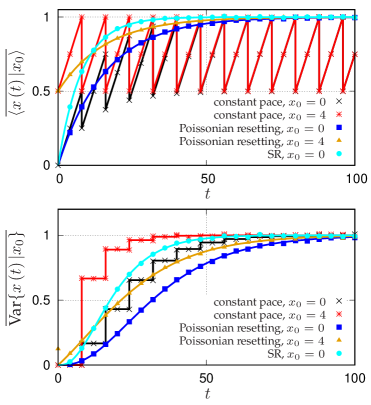
Figure 7: Mean and variance of the height profile for dependent stochastic resetting with Poissonian [$r=0.125$, Eqs. (78) and (79)] and constant pace [Eqs. (68) and (71)] resetting times for uniform resetting amplitude and two different initial heights $x_{0}$, in comparison with classical resetting (SR). We plot both quantities according to the normalization in Eqs. (80) and (81). The propagating process is ballistic ($v=0.5$) in all cases. Numerical results are shown by points, the analytical results by solid lines.

For Poissonian resetting times both mean and variance become independent of the initial height in the long time limit. The functional behavior of both quantities for Poissonian and constant pace resetting times are shown in Fig. 7, in which we use the nomalized expressions

$$\overline{\langle x(t)|x_{0}\rangle} = \frac{\langle x(t)|x_{0}\rangle}{\underset{t\to\infty}{\limsup}\langle x(t)|x_{0}\rangle},$$ (80)

$$\overline{\mathrm{Var}\{x(t)|x_{0}\}} = \frac{\mathrm{Var}\{x(t)|x_{0}\}}{\underset{t\to\infty}{\lim}\mathrm{Var}\{x(t)|x_{0}\}}.$$ (81)

In this asymptotic limit the normalized mean converges to unity for Poissonian resetting. In contrast, with constant pace resetting times the oscillating quantity $\overline{\langle x(t)|x0\rangle}$ is limited from above by unity. Based on definition (80) of the normalized mean, the two different convergence behaviors are compared in the upper panel of Fig. 7. The normalized variance in Eq. (81) has the same limiting value for both Poissonian and constant pace resetting, see the lower panel of Fig. 7.

IV.5 Derivation of the probability density $P(x,t)$ for Poissonian resetting, ballistic propagation and dependent resetting amplitudes

To derive a differential equation for the PDF $P(x,t;x_{0};t_{0})$ we use the fact that the process is homogeneous in time and derived the master equation for $P(x,t;x_{0})$, for which $(x(t+\Delta t)|x_{0})=c(x(t)|x_{0})$ with probability $r\Delta t$ and $(x(t+\Delta t)|x_{0})=x(t)|x_{0})+v\Delta t$ with probability $1-r\Delta t$,

$$\frac{\partial P(x,t;x_{0})}{\partial t}=-v\frac{\partial P(x,t;x_{0})}{\partial x}-rP(x,t;x_{0})+r\int\limits_{0}^{\infty}\frac{dy}{y}P(y,t;x_{0})f_{C}\left(\frac{x}{y}\right),$$ (82)

with $P(x,0;x_{0})=\delta(x-x_{0})$. For the Laplace transform $\bar{P}(u,t;x_{0})$ of $P(x,t;x_{0})$ with respect to $x$ this yields

$$\frac{\partial\bar{P}(u,t;x_{0})}{\partial t}=-uv\bar{P}(u,t;x_{0})-r\bar{P}(u,t;x_{0})+r\int\limits_{0}^{1}dc\bar{P}(uc,t;x_{0})f_{C}(c)$$ (83)

with $\bar{P}(u,0;x_{0})=\exp(-ux_{0})$.

IV.5.1 Comparison with classical Stochastic Resetting

If we assume a standard SR to the initial condition $x_{0}$ we have $f_{C}(c)=\delta(c)$. Moreover, the relation of the corresponding random variable, and thus the partial differential is slightly different. Explicitly, $(x(t+\Delta t)|x_{0})=c\times(x(t)|x_{0})+x_{0}$ with probability $r\Delta t$ and $(x(t+\Delta t)|x_{0})=(x(t)|x_{0})+v\Delta t$ with probability $1-r\Delta t$, thus

$$\frac{\partial P(x,t;x_{0})}{\partial t} = -v\frac{\partial P(x,t;x_{0})}{\partial x}-rP(x,t;x_{0})+r\int_{0}^{\infty}\frac{P(y,t;x_{0})}{y}\delta\left(\frac{x-x_{0}}{y}\right)dy$$ (84)

$$= \frac{\partial P(x,t;x_{0})}{\partial t}=-v\frac{\partial P(x,t;x_{0})}{\partial x}-rP(x,t;x_{0})+r\delta(x-x_{0})$$

where $P(x,0;x_{0})=\delta(x-x_{0})$ and we used the condition that $P(x,t;x_{0})$ is normalized and the scaling property of the delta function, $\delta(ax)=\delta(x)/|a|$ for $a\in\mathbb{R}$. Finally, in the case of SR with an arbitrary initial distribution $\phi_{0}(x)$ the distribution of $x$ at time $t$ can be computed from $\rho(x,t)=\int_{0}^{\infty}\phi_{0}(x_{0})P(x,t;x_{0})dx_{0}$ and we get

$$\frac{\partial\rho(x,t)}{\partial t}=-v\frac{\partial\rho(x,t)}{\partial x}-r\rho(x,t)+r\phi_{0}(x)$$ (85)

with $\rho(x,0)=\phi_{0}(x)$. Eq. (84) is homogeneous in space and confirms the results of Ref. Evans1 for ballistic displacement instead of a diffusive displacement.

IV.5.2 Stationary distribution for ballistic displacement, uniform dependent resetting amplitude and Poissonian resetting

We get the stationary solution of Eq. (83) for $f_{C}(c)=1$ with $P^{*}(x)=\underset{t\to\infty}{\lim}P(x,t;x_{0})$ for $\lim_{t\to\infty}\partial P(x,t;x_{0})/\partial t=0$. Thus, for the spatial Laplace transform $\bar{P}^{*}(u)$ becomes

$$0=-uv\bar{P}^{*}(u)-r\bar{P}^{*}(u)+r\int_{0}^{1}\bar{P}^{*}(uc)dc,\quad\Leftrightarrow\quad u(uv+r)\bar{P}^{*}(u)=r\int_{0}^{u}\bar{P}^{*}(c^{\prime})dc^{\prime},$$ (86)

with $c^{\prime}=uc$. If we now differentiate Eq. (86) with respect to $u$ and use the normalization condition $\bar{P}^{*}(0)=1$, we get

$$(2uv+r)\bar{P}^{*}(u)+u(uv+r)\bar{P}^{*^{\prime}}(u)=r\bar{P}^{*}(u),$$ (87)

implying $\bar{P}^{*^{\prime}}(u)=\frac{2v}{uv+r}\bar{P}^{*}(u)$ and $\bar{P}^{*}(0)=1$. The solution is given by

$$\bar{P}^{*}(u)=\frac{r^{2}}{(uv+r)^{2}}.$$ (88)

Eq. (88) solves Eq. (86), which proves our claim.

Thus, the stationary solution $P^{*}(x)$ is the inverse Laplace transform of $\bar{P}^{*}(u)$, Eq. (88),

$$P^{*}(x)=\lim_{t\to\infty}P(x,t;x_{0})=\left(\frac{r}{v}\right)^{2}x\exp\left(-\frac{rx}{v}\right).$$ (89)

IV.5.3 Proof of equality between partial differential equation (83) and integral representation (62)

Let $\tilde{\bar{P}}(u,s)$ denote the Laplace transform of $\bar{P}(u,t)$, we can obtain the following forms for Poissonian resetting in double-Laplace space,

$$\tilde{\bar{P}}(u,s;x_{0})=\frac{\exp(-ux_{0})}{r+s+uv}+\frac{r}{r+s+uv}\int\limits_{0}^{1}dc\tilde{\bar{P}}(uc,s;x_{0})f_{C}(c)$$ (90)

with the following iterative approximations

$$0\mbox{th approximation}=\frac{\exp(-ux_{0})}{r+s+uv}$$

$$1\mbox{st approximation}=\frac{\exp(-ux_{0})}{r+s+uv}+\frac{r}{r+s+uv}\int\limits_{0}^{1}dc\frac{\exp(-ux_{0}c)}{r+s+uvc})f_{C}(c)$$

$$2\mbox{nd approximation}=\frac{\exp(-ux_{0})}{r+s+uv}+\frac{r}{r+s+uv}\int\limits_{0}^{1}dc_{1}\frac{\exp(-ux_{0}c_{1})}{r+s+uvc_{1}}f_{C}(c_{1})$$

$$+\frac{r}{r+s+uv}\int\limits_{0}^{1}dc_{1}\frac{rf_{C}(c_{1})}{r+s+uvc_{1}}\int\limits_{0}^{1}dc_{2}\frac{\exp(-ux_{0}c_{1}c_{2})f_{C}(c_{2})}{r+s+uvc_{1}c_{2}}$$

$$n\mbox{th approximation}=\frac{\exp(-ux_{0})}{r+s+uv}+\frac{1}{r+s+uv}\sum^{n}_{m=1}\left(\prod^{m}_{j=1}\int\limits_{0}^{1}dc_{j}\frac{rf_{C}(c_{j})}{\left(r+s+uv\prod^{j}_{i=1}c_{i}\right)}\right)\exp\left(-x_{0}\prod^{m}_{j=1}c_{j}\right)$$

such that we find

$$\tilde{\bar{P}}(u,s;x_{0})=\frac{\exp(-ux_{0})}{r+s+uv}+\frac{1}{r+s+uv}\sum^{\infty}_{n=1}\left(\prod^{n}_{j=1}\int\limits_{0}^{1}dc_{j}\frac{rf_{C}(c_{j})}{\left(r+s+uv\prod^{j}_{i=1}c_{i}\right)}\right)\exp\left(-x_{0}\prod^{n}_{j=1}c_{j}\right),$$ (91)

which is equal to Eq. (62) for Poissonian resetting, and thus proves our claim.

IV.6 Graphical illustration for dependent resetting

We finally illustrate the difference between ballistic propagation with Poissonian and constant pace resetting for uniform dependent resetting amplitude. To this end we compare the corresponding PDFs at different times respectively show the behavior of mean and variance of $(x(t)|x_{0})$.

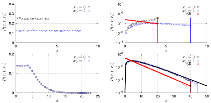
Figure 8: PDF $P(x,t;x_{0})$ of the height profile for different initial heights and ballistic motion with uniform resetting. Left: "constant pace" resetting. Right: Poissonian resetting, compared to the classical resetting scenario with enforced resets to the origin. Top: $t=1/r$. Bottom: $t=10/r$. Numerical results are shown by points, analytical results by solid lines. Parameters: $v=0.5$ and $r=0.125$.

Fig. 8 shows the position PDF for ballistic displacement, uniformly distributed resetting amplitude and two different distributions of resetting interval lengths. For each process the impact of different initial values $x_{0}$ is shown. It is obvious that the influence of initial values eventually disappears, as can be seen in the upper panels. In the left panel of Fig. 8 constant pace resetting is used. When the impact of the initial value disappears (lower left panel) the PDF of $x$ has a uniform part for small values of $x$. However, the uniform character disappears from a certain value of $x$ and decreases in the tail. The distribution does not change its shape, however, the PDF of $x$ fulfills a periodic movement. This motion of the distribution $P(x,t;x_{0})$ is divided in a linear shift in time and a shift in the opposite direction as a point process in time. In the right panels of Fig. 8 Poissonian resetting is used. The height of the probability of no resets is independent of the value of $x_{0}$. This probability is mapped at $x=vt+x_{0}$ and decreasing in time. For longer $t$ (right lower panel) it can be seen that the process is stationary.

In Fig. 9 we can see the temporal behavior of the average and variance of $(x(t)|x_{0})$. We show the results for ballistic displacement process which is interrupted by uniform dependent resetting events for two different distributions of resetting interval lengths. All analytical results are numerically verified, see Fig. 9. The vanishing impact of different initial values $x_{0}$ for average and variance of $(x(t)|x_{0})$ with $t$ can be seen in all panels. The average $\langle x(t)|x_{0}\rangle$ (left upper panel) increases linearly with $t$ during the constant resetting interval lengths and decreases at the resetting points. After some time the average of $(x(t)|x_{0})$ is confined to a certain range and has a periodic switch between linear increase and decrease as a point process in time. The corresponding $\mathrm{Var}\{x(t)|x_{0}\}$ (left lower panel) stays the same during the resetting interval lengths and increases discontinuously at the resetting points, a jump in the figure. For longer $t$ the variance $\mathrm{Var}\{x(t)|x_{0}\}$ converges to a finite limit. In the right panels of Fig. 9 the convergence of average and variance of $(x(t)|x_{0})$ in presence of Poissonian resetting is obvious. Thus, this process is stationary.

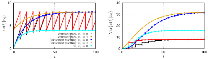
Figure 9: Mean $\langle x(t)|x_{0}\rangle$ and variance $\mathrm{Var}\{x(t)|x_{0}\}$ of the height profile for dependent stochastic resetting with Poissonian and "constant pace" resetting times for uniform resetting amplitude and two different initial heights $x_{0}$, in comparison with classical resetting. The propagating process is ballistic ($v=0.5$) in all cases. For both types of resetting the resetting rate is $r=0.125$. Numerical results are shown by points, the analytical results by lines.

Fig. 10 shows the PDF for ballistic propagation with Poissonian resetting times for classical resetting to the origin and uniform resetting amplitudes, for two different initial heights $x_{0}$. At early times of the process (top panel) the difference due to the initial height is distinct, while in the long time limit (bottom panel) the PDFs for the two uniform-resetting cases coincide. The difference to the classical resetting case with enforced resetting to the origin clearly results in a lower height profile.

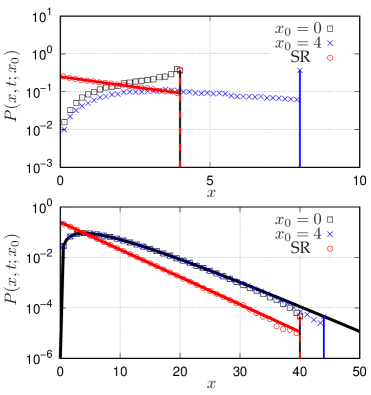
Figure 10: PDF $P(x,t;x_{0})$ of the height profile for different initial heights and uniform resetting amplitude, compared to the classical resetting scenario with enforced resets to the origin, for ballistic propagation ($v=0.5$) and Poissonian resetting times ($r=0.125$). Top: $t=1/r$; bottom: $t=10/r$. Numerical results are shown by points, analytical results by lines.

V Conclusions

We introduced a generalized resetting concept with random resetting amplitudes in two different scenarios: independent resetting, in which the height profile may become negative, depending on the specific resetting amplitude PDF and the propagating process; and dependent resetting, in which the positivity of the height profile is guaranteed by the definition of the resetting amplitude PDF. We derived an explicit analytical formulation of the process and analyzed specifically ballistic propagation in the presence of Poissonian resetting times and different resetting amplitude PDFs. We also demonstrated that the classical resetting theory with mandatory resets to the origin is contained in our model in the dependent case, whereas the independent scenario is a specific case of jump diffusion Kou with one-sided jump lengths.

Physically, the RASR process introduce here corresponds to the scenario of a propagating stochastic or deterministic process, that is interrupted by random resets. This may correspond to the geophysical stratigraphic scenario, in which the propagation mimics the gradual build-up or decay of a sedimentation profile, whereas the resets represent sudden erosion events. The latter could be seasonal ("constant pace") or random-in-time weather events such as extreme floods. In fact our model is similar (albeit more flexible) to that proposed in SD_6 , where constant rates of accumulation were considered the null hypothesis and the effect of random erosion periods on bed hiatus length distributions were explored. We also note similar strategies developed for ecohydrology applications iturbe , and the general development of a class of jump processes porporato . In a different context we could think of population dynamics interrupted by epidemics, pathogens (e.g., embodied by bacterial biofilms) decimated by antibiotic treatment (here, both periodic and "random" application protocols are being employed in clinical studies), or crises-interrupted financial markets. All these cases process correspond to the intermittent picture of a parent process (the "propagation") with superimposed resetting statistic.

The qualitative difference between independent and dependent resetting is that the latter case becomes stationary for ballistic propagation and Poissonian resetting times, whereas the former remains non-stationary. The fact that our basic model can be recast in these two variants underlines the flexibility embedded in this simple extension of classical resetting (SR). Another appeal is the relatively straightforward, fully analytical description, with the caveat that not all resulting expressions can be expressed fully explicitly. Having said this, we believe that our results represent an attractive extension of the resetting process. Apart from the above physical scenarios the described flexibility of our extension of the resetting dynamics will be of interest in the mathematical theory of random search processes.

Appendix A Mathematical identity between first and last resetting picture

In this section we prove the following formal mathematical identity that will be used in Appendix B below to demonstrate the equivalence of the first and the last resetting pictures:

$$\prod^{n}_{j=1}\left(\int_{t_{j-1}}^{t}dt_{j}\int_{A_{1}}^{A_{2}}dy_{j}\int_{A_{3}}^{A_{4}}dz_{j}\eta_{1}(t_{j},t_{j-1},y_{j},y_{j-1},z_{j},z_{j-1})\right)\eta_{2}(x,t,t_{n},y_{n},z_{n})$$

$$=\int_{0}^{t-t_{0}}d\tau_{n}\int_{A_{1}}^{A_{2}}dy_{n}\int_{A_{3}}^{A_{4}}dz_{n}\left(\prod^{n-1}_{i=1}\int_{0}^{\tau_{n+1-i}}d\tau_{n-i}\int_{A_{1}}^{A_{2}}dy_{n-i}\int_{A_{3}}^{A_{4}}dz_{n-i}\right.$$

$$\times\eta_{1}(\tau_{n+1-i}+t_{0},\tau_{n-i}+t_{0},y_{n+1-i},y_{n-i},z_{n+1-i},z_{n-i})\Big{)}$$

$$\times\eta_{1}(\tau_{1}+t_{0},t_{0},y_{1},y_{0},z_{1},z_{0})\eta_{2}(x,t,\tau_{n}+t_{0},y_{n},z_{n})$$

$$\Leftrightarrow\prod^{n}_{j=1}\left(\int_{\tau_{j-1}}^{t-t_{0}}d\tau_{j}\int^{A_{2}}_{A_{1}}dy_{j}\int^{A_{4}}_{A_{3}}dz_{j}\eta_{1}(\tau_{j}+t_{0},\tau_{j-1}+t_{0},y_{j},y_{j-1},z_{j},z_{j-1})\right)\eta_{2}(x,t,\tau_{n}+t_{0},y_{n},z_{n})$$

$$=\int_{0}^{t-t_{0}}d\tau_{n}\int_{A_{1}}^{A_{2}}dy_{n}\int_{A_{3}}^{A_{4}}dz_{n}\left(\prod^{n-1}_{i=1}\int_{0}^{\tau_{n+1-i}}d\tau_{n-i}\int_{A_{1}}^{A_{2}}dy_{n-i}\int_{A_{3}}^{A_{4}}dz_{n-i}\right.$$

$$\times\eta_{1}(\tau_{n+1-i}+t_{0},\tau_{n-i}+t_{0},y_{n+1-i},y_{n-i},z_{n+1-i},z_{n-i})\Big{)}$$

$$\times\eta_{1}(\tau_{1}+t_{0},t_{0},y_{1},y_{0},z_{1},z_{0})\eta_{2}(x,t,\tau_{n}+t_{0},y_{n},z_{n})$$ (92)

with $\tau_{j}=t_{j}-t_{0}$ for $0\leq j\leq n$. To prove Eq. (92) we use the method of induction. For $n=1$, the Eq. (92) is obviously fulfilled,

$$\int_{0}^{t-t_{0}}d\tau_{1}\int_{A_{1}}^{A_{2}}dy_{1}\int_{A_{3}}^{A_{4}}dz_{1}\eta_{1}(\tau_{1}+t_{0},t_{0},y_{1},y_{0},z_{1},z_{0})\eta_{2}(x,t,\tau_{1}+t_{0},y_{1},z_{1})$$

$$=\int_{0}^{t-t_{0}}d\tau_{1}\int_{A_{1}}^{A_{2}}dy_{1}\int_{A_{3}}^{A_{4}}dz_{1}\eta_{1}(\tau_{1}+t_{0},t_{0},y_{1},y_{0},z_{1},z_{0})\eta_{2}(x,t,\tau_{1}+t_{0},y_{1},z_{1}).$$ (93)

Next, we take the inductive step $n\Rightarrow(n+1)$,

$$\prod^{n+1}_{j=1}\left(\int\limits_{\tau_{j-1}}^{t-t_{0}}d\tau_{j}\int\limits_{A_{1}}^{A_{2}}dy_{j}\int\limits_{A_{3}}^{A_{4}}dz_{j}\eta_{1}(\tau_{j}+t_{0},\tau_{j-1}+t_{0},y_{j},y_{j-1},z_{j},z_{j-1})\right)\eta_{2}(x,t,\tau_{n+1}+t_{0},y_{n+1},z_{n+1})$$

$$=\int\limits_{\tau_{n}}^{t-t_{0}}d\tau_{n+1}\int\limits_{A_{1}}^{A_{2}}dy_{n+1}\int\limits_{A_{3}}^{A_{4}}dz_{n+1}\eta_{1}(\tau_{n+1}+t_{0},\tau_{n}+t_{0},y_{n+1},y_{n},z_{n+1},z_{n})$$

$$\times\prod^{n}_{j=1}\left(\int\limits_{\tau_{j-1}}^{t-t_{0}}d\tau_{j}\int\limits_{A_{1}}^{A_{2}}dy_{j}\int\limits_{A_{3}}^{A_{4}}dz_{j}\eta_{1}(\tau_{j}+t_{0},\tau_{j-1}+t_{0},y_{j},y_{j-1},z_{j},z_{j-1})\right)\eta_{2}(x,t,\tau_{n+1}+t_{0},y_{n+1},z_{n+1}),$$

i.e.,

$$\int\limits_{0}^{t-t_{0}}d\tau_{n}\int\limits_{\tau_{n}}^{t-t_{0}}d\tau_{n+1}\int\limits_{A_{1}}^{A_{2}}dy_{n}\int\limits_{A_{3}}^{A_{4}}dz_{n}$$

$$\times\left(\prod^{n-1}_{i=1}\int\limits_{0}^{\tau_{n+1-i}}d\tau_{n-i}\int\limits_{A_{1}}^{A_{2}}dy_{n-i}\int\limits_{A_{3}}^{A_{4}}dz_{n-i}\eta_{1}(\tau_{n+1-i}+t_{0},\tau_{n-i}+t_{0},y_{n+1-i},y_{n-i},z_{n+1-i},z_{n-i})\right)$$

$$\times\int\limits_{A_{1}}^{A_{2}}dy_{n+1}\int\limits_{A_{3}}^{A_{4}}dz_{n+1}\eta_{1}(\tau_{n+1}+t_{0},\tau_{n}+t_{0},y_{n+1},y_{n},z_{n+1},z_{n})\eta_{1}(\tau_{1}+t_{0},t_{0},y_{1},y_{0},z_{1},z_{0})\eta_{2}(x,t,\tau_{n}+t_{0},y_{n},z_{n})$$

$$=\int\limits_{0}^{t-t_{0}}d\tau_{n+1}\int\limits_{0}^{\tau_{n+1}}d\tau_{n}\int\limits_{A_{1}}^{A_{2}}dy_{n}\int\limits_{A_{3}}^{A_{4}}dz_{n}$$

$$\times\left(\prod^{n}_{i=2}\int\limits_{0}^{\tau_{n+2-i}}d\tau_{n+1-i}\int\limits_{A_{1}}^{A_{2}}dy_{n+1-i}\int\limits_{A_{3}}^{A_{4}}dz_{n+1-i}\eta_{1}(\tau_{n+2-i}+t_{0},\tau_{n+1-i}+t_{0},y_{n+2-i},y_{n+1-i},z_{n+2-i},z_{n+1-i})\right)$$

$$\times\int\limits_{A_{1}}^{A_{2}}dy_{n+1}\int\limits_{A_{3}}^{A_{4}}dz_{n+1}\eta_{1}(\tau_{n+1}+t_{0},\tau_{n}+t_{0},y_{n+1},y_{n},z_{n+1},z_{n})\eta_{1}(\tau_{1}+t_{0},t_{0},y_{1},y_{0},z_{1},z_{0})\eta_{2}(x,t,\tau_{n}+t_{0},y_{n},z_{n})$$

$$=\int\limits_{0}^{t-t_{0}}d\tau_{n+1}\int\limits_{A_{1}}^{A_{2}}dy_{n+1}\int\limits_{A_{3}}^{A_{4}}dz_{n+1}$$

$$\times\left(\prod^{n}_{i=1}\int\limits_{0}^{\tau_{n+2-i}}d\tau_{n+1-i}\int\limits_{A_{1}}^{A_{2}}dy_{n+1-i}\int\limits_{A_{3}}^{A_{4}}dz_{n+1-i}\eta_{1}(\tau_{n+2-i}+t_{0},\tau_{n+1-i}+t_{0},y_{n+2-i},y_{n+1-i},z_{n+2-i},z_{n+1-i})\right)$$

$$\times\eta_{1}(\tau_{1}+t_{0},t_{0},y_{1},y_{0},z_{1},z_{0})\eta_{2}(x,t,\tau_{n}+t_{0},y_{n},z_{n}).$$ (94)

This proves our claim.

Appendix B Derivation of last resetting picture for independent resetting amplitudes

In this section we aim to show the equivalence of the description in the first resetting picture,

$$P(x,t;x_{0},t_{0})=\Psi(t-t_{0})G(x,t;x_{0},t_{0})+\int\limits_{t_{0}}^{t}dt_{1}\psi(t_{1}-t_{0})\int\limits_{-\infty}^{\infty}dyG(y,t_{1};x_{0},t_{0})\int\limits_{-\infty}^{\infty}dx_{1}q\left(x_{1}-y\right)P(x,t;x_{1},t_{1})$$ (95)

and the last resetting picture that includes all resetting steps,

$$P(x,t;x_{0},t_{0})=\Psi(t-t_{0})G(x,t;x_{0},t_{0})+\sum^{\infty}_{n=1}\int\limits_{0}^{t-t_{0}}d\tau_{n}\int\limits_{-\infty}^{\infty}dx_{n}\int\limits_{-\infty}^{\infty}dy_{n}$$

$$\times\left(\prod^{n-1}_{i=1}\int\limits_{0}^{\tau_{n+1-i}}d\tau_{n-i}\psi(\tau_{n+1-i}-\tau_{n-i})\int\limits_{-\infty}^{\infty}dy_{n-i}G(y_{n+1-i},\tau_{n+1-i}+t_{0};x_{n-i},\tau_{n-i}+t_{0})\int\limits_{-\infty}^{\infty}dx_{n-i}q\left(x_{n+1-i}-y_{n+1-i}\right)\right)$$

$$\times q\left(x_{1}-y_{1}\right)\psi(\tau_{1})G(y_{1},\tau_{1}+t_{0};x_{0},t_{0})\Psi(t-t_{0}-\tau_{n})G(x,t;x_{n},\tau_{n}+t_{0}).$$ (96)

To this end we write Eq. (96) as

$$P(x,t;x^{\prime},t^{\prime})=\Psi(t-t^{\prime})G(x,t;x^{\prime},t^{\prime})+$$

$$+\sum^{\infty}_{n=1}\left(\prod^{n}_{j=1}\int\limits_{t_{j-1}}^{t}dt_{j}\psi(t_{j}-t_{j-1})\int\limits_{-\infty}^{\infty}dy_{j}G(y_{j},t_{j};x_{j-1},t_{j-1})\int\limits_{-\infty}^{\infty}dx_{j}q\left(x_{j}-y_{j}\right)\right)\Psi(t-t_{n})G(x,t;x_{n},t_{n})$$ (97)

with $t_{0}=t^{\prime}$ and $x_{0}=x^{\prime}$. The equivalence of Eqs.(96) and (97) will be proven in this section below. Now we substitute $P(x,t;x_{0},t_{0})$ and $P(x,t;x_{1},t_{1})$ in the first resetting picture, Eq. (95) with Eq. (97). The left hand side (LHS) of Eq. (95) after this substitution becomes

$$\text{LHS}=P(x,t;x_{0},t_{0})=\Psi(t-t_{0})G(x,t;x_{0},t_{0})+$$

$$+\sum^{\infty}_{n=1}\left(\prod^{n}_{j=1}\int\limits_{t_{j-1}}^{t}dt_{j}\psi(t_{j}-t_{j-1})\int\limits_{-\infty}^{\infty}dy_{j}G(y_{j},t_{j};x_{j-1},t_{j-1})\int\limits_{-\infty}^{\infty}dx_{j}q\left(x_{j}-y_{j}\right)\right)\Psi(t-t_{n})G(x,t;x_{n},t_{n}).$$ (98)

As $P(x,t;x_{1},t_{1})$ in Eq. (95) has the initial value $x_{1}$ at $t_{1}$, these two variables have the lowest index $1$ instead of $0$, and thus instead of Eq. (98) one gets

$$P(x,t;x_{1},t_{1})=\Psi(t-t_{1})G(x,t;x_{1},t_{1})$$

$$+\sum^{\infty}_{n=2}\left(\prod^{n}_{j=2}\int\limits_{t_{j-1}}^{t}dt_{j}\psi(t_{j}-t_{j-1})\int\limits_{-\infty}^{\infty}dy_{j}G(y_{j},t_{j};x_{j-1},t_{j-1})\int\limits_{-\infty}^{\infty}dx_{j}q(x_{j}-y_{j})\right)\Psi(t-t_{n})G(x,t;x_{n},t_{n}).$$ (99)

Substituting (99) into the RHS of Eq. (95) we get

$$\mathrm{RHS}=\Psi(t-t_{0})G(x,t;x_{0},t_{0})$$

$$+\int\limits_{t_{0}}^{t}dt_{1}\psi(t_{1}-t_{0})\int\limits_{-\infty}^{\infty}dyG(y,t_{1};x_{0},t_{0})\int\limits_{-\infty}^{\infty}dx_{1}q(x_{1}-y)\Psi(t-t_{1})G(x,t;x_{1},t_{1})$$

$$+\int\limits_{t_{0}}^{t}dt_{1}\int\limits_{-\infty}^{\infty}dy\int\limits_{-\infty}^{\infty}dx_{1}\sum^{\infty}_{n=2}\left(\prod^{n}_{j=2}\int\limits_{t_{j-1}}^{t}dt_{j}\psi(t_{j}-t_{j-1})\int\limits_{-\infty}^{\infty}dy_{j}G(y_{j},t_{j};x_{j-1},t_{j-1})\int\limits_{-\infty}^{\infty}dx_{j}q\left(x_{j}-y_{j}\right)\right)$$

$$\times\psi(t_{1}-t_{0})G(y,t_{1};x_{0},t_{0})q(x_{1}-y)\Psi(t-t_{n})G(x,t;x_{n},t_{n})$$

$$= \Psi(t-t_{0})G(x,t;x_{0},t_{0})$$ (100)

$$+\int\limits_{t_{0}}^{t}dt_{1}\psi(t_{1}-t_{0})\int\limits_{-\infty}^{\infty}dy_{1}G(y_{1},t_{1};x_{0},t_{0})\int\limits_{-\infty}^{\infty}dx_{1}q(x_{1}-y_{1})\Psi(t-t_{1})G(x,t;x_{1},t_{1})$$

$$+\sum^{\infty}_{n=2}\left(\prod^{n}_{j=1}\int\limits_{t_{j-1}}^{t}dt_{j}\psi(t_{j}-t_{j-1})\int\limits_{-\infty}^{\infty}dy_{j}G(y_{j},t_{j};x_{j-1},t_{j-1})\int\limits_{-\infty}^{\infty}dx_{j}q(x_{j}-y_{j})\right)\Psi(t-t_{n})G(x,t;x_{n},t_{n})$$

with $y_{1}=y$. Then,

$$\mathrm{RHS}=\Psi(t-t_{0})G(x,t;x_{0},t_{0})$$

$$+ \sum^{\infty}_{n=1}\left(\prod^{n}_{j=1}\int\limits_{t_{j-1}}^{t}dt_{j}\psi(t_{j}-t_{j-1})\int\limits_{-\infty}^{\infty}dy_{j}G(y_{j},t_{j};x_{j-1},t_{j-1})\int\limits_{-\infty}^{\infty}dx_{j}q(x_{j}-y_{j})\right)\Psi(t-t_{n})G(x,t;x_{n},t_{n}),$$ (101)

and thus $\mathrm{RHS}=\mathrm{LHS}$, which proves our claim. Thus, Eq. (97) solves the first resetting picture of Eq. (95), and Eq. (97) describes the RASR with independent resetting amplitudes. If we can show that Eq. (97) and the last resetting picture of Eq. (96) are equal, we demonstrate that both mathematical representations describe the same process. To this end, consider

$$\mathrm{LHS}=P(x,t;x_{0},t_{0})=\Psi(t-t_{0})G(x,t;x_{0},t_{0})$$

$$+\sum^{\infty}_{n=1}\left(\prod^{n}_{j=1}\int\limits_{t_{j-1}}^{t}dt_{j}\psi(t_{j}-t_{j-1})\int\limits_{-\infty}^{\infty}dy_{j}G(y_{j},t_{j};x_{j-1},t_{j-1})\int\limits_{-\infty}^{\infty}dx_{j}q(x_{j}-y_{j})\right)\Psi(t-t_{n})G(x,t;x_{n},t_{n})$$

$$=\Psi(t-t_{0})G(x,t;x_{0},t_{0})$$

$$+\sum^{\infty}_{n=1}\left(\prod^{n}_{j=1}\int\limits_{\tau_{j-1}}^{t-t_{0}}d\tau_{j}\psi(\tau_{j}-\tau_{j-1})\int\limits_{-\infty}^{\infty}dy_{j}G(y_{j},\tau_{j}+t_{0};x_{j-1},\tau_{j-1}+t_{0})\int\limits_{-\infty}^{\infty}dx_{j}q(x_{j}-y_{j})\right)$$

$$\times\Psi(t-\tau_{n})G(x,t;x_{n},\tau_{n}+t_{0}),$$ (102)

with $\tau_{j}=t_{j}-t_{0}$ for $1\leq j\leq n$.

If we now use Eq. (92) with the substitution (107), we obtain

$$\left\{\begin{array}[]{lllll}\eta_{1}(t_{j},t_{j-1},y_{j},y_{j-1},z_{j},z_{j-1})=\psi(t_{j}-t_{j-1})G(y_{j},t_{j};z_{j-1},t_{j-1})q(z_{j}-y_{j})\\[5.69046pt] \eta_{2}(x,t,t_{n},y_{n},z_{n})=\Psi(t-t_{0})G(x,t;z_{n},t_{n})\\[5.69046pt] z_{j}=x_{j},\,\,\,t_{j}=\tau_{j}+t_{0}\\[5.69046pt] A_{1},A_{3}=-\infty,\,\,\,A_{2},A_{4}=\infty\end{array}\right.,$$ (107)

for $1\leq j\leq n$. We then find

$$\text{LHS}=\Psi(t-t_{0})G(x,t;x_{0},t_{0})+\sum^{\infty}_{n=1}\int\limits_{0}^{t-t_{0}}d\tau_{n}\int\limits_{-\infty}^{\infty}dx_{n}\int\limits_{-\infty}^{\infty}dy_{n}\left(\prod^{n-1}_{i=1}\int\limits_{0}^{\tau_{n+1-i}}d\tau_{n-i}\psi(\tau_{n+1-i}-\tau_{n-i})\right)$$

$$\times\left(\prod^{n-1}_{i=1}\int\limits_{-\infty}^{\infty}dy_{n-i}G(y_{n+1-i},\tau_{n+1-i}+t_{0};x_{n-i},\tau_{n-i}+t_{0})\int\limits_{-\infty}^{\infty}dx_{n-i}q(x_{n+1-i}-y_{n+1-i})\right)$$

$$\times q(x_{1}-y_{1})\psi(\tau_{1})G(y_{1},\tau_{1}+t_{0};x_{0},t_{0})\Psi(t-t_{0}-\tau_{n})G(x,t;x_{n},\tau_{n}+t_{0}),$$ (108)

which represents exactly the last resetting picture (96), proving our claim.

If we assume a free propagator, that is homogeneous in space and in time, the stochastic process with resetting itself will be homogeneous in space and time, $G(x,t;x_{0},t_{0})=G(x-x_{0},t-t_{0};0,0)\Rightarrow P(x,t;x_{0},t_{0})=P(x-x_{0},t-t_{0};0,0)$. By assuming $G(x,t;x_{0},t_{0})=G(x-x_{0},t-t_{0};0,0)$ the density $P(x,t;x_{0},t_{0})$, Eq. (108), then becomes

$$P(x,t;x_{0},t_{0})=\Psi(t-t_{0})G(x-x_{0},t-t_{0};0,0)+\sum^{\infty}_{n=1}\int\limits_{0}^{t-t_{0}}d\tau_{n}\int\limits_{-\infty}^{\infty}dx_{n}\int\limits_{-\infty}^{\infty}dy_{n}$$

$$\times\left(\prod^{n-1}_{i=1}\int\limits_{0}^{\tau_{n+1-i}}d\tau_{n-i}\psi(\tau_{n+1-i}-\tau_{n-i})\int\limits_{-\infty}^{\infty}dy_{n-i}G(y_{n+1-i}-x_{n-i},\tau_{n+1-i}-\tau_{n-i};0,0)\int\limits_{-\infty}^{\infty}dx_{n-i}q\left(x_{n+1-i}-y_{n+1-i}\right)\right)$$

$$\times q\left(x_{1}-y_{1}\right)\psi(\tau_{1})G(y_{1}-x_{0},\tau_{1};0,0)\Psi(t-t_{0}-\tau_{n})G(x-x_{n},t-t_{0}-\tau_{n};0,0),$$

$$=\Psi(t-t_{0})G(x-x_{0},t-t_{0};0,0)+\sum^{\infty}_{n=1}\int\limits_{0}^{t-t_{0}}d\tau_{n}\int\limits_{-\infty}^{\infty}dx^{\prime}_{n}\int\limits_{-\infty}^{\infty}dy^{\prime}_{n}$$

$$\times\left(\prod^{n-1}_{i=1}\int\limits_{0}^{\tau_{n+1-i}}d\tau_{n-i}\psi(\tau_{n+1-i}-\tau_{n-i})\int\limits_{-\infty}^{\infty}dy^{\prime}_{n-i}G(y^{\prime}_{n+1-i}-x^{\prime}_{n-i},\tau_{n+1-i}-\tau_{n-i};0,0)\int\limits_{-\infty}^{\infty}dx^{\prime}_{n-i}q\left(x^{\prime}_{n+1-i}-y^{\prime}_{n+1-i}\right)\right)$$

$$\times q\left(x^{\prime}_{1}-y^{\prime}_{1}\right)\psi(\tau_{1})G(y^{\prime}_{1},\tau_{1};0,0)\Psi(t-t_{0}-\tau_{n})G(x-x_{0}-x^{\prime}_{n},t-t_{0}-\tau_{n};0,0),$$ (109)

in which $x^{\prime}_{j}=x_{j}-x_{0}$ and $y^{\prime}_{j}=y_{j}-x_{0}$ for $1\leq j\leq n$. On the right hand side of Eq. (B) $x$ and $x_{0}$ as well as $t$ and $t_{0}$ only occur as differences $x-x_{0}$ and $t-t_{0}$ and not as single terms. Thus, $G(x,t;x_{0},t_{0})=G(x-x_{0},t-t_{0};0,0)\Rightarrow P(x,t;x_{0},t_{0})=P(x-x_{0},t-t_{0};0,0)$, which proves our claim.

Appendix C Differential equation for $P(x,t)$ with Poissonian resetting, ballistic displacement process, and arbitrary independent resetting amplitudes

To derive a differential equation for the PDF $P(x,t;x_{0};t_{0})$ we use the fact that the process is homogeneous in space and time. We use the short-hand form $P(x,t)$ for the choice $x(t_{0}=0)=0$. As the $x$-propagation for ballistic motion reads

$$x(t+\Delta t)=\left\{\begin{array}[]{ll}x(t)+z\mbox{ with probability }r\Delta t\\ x(t)+v\Delta t\mbox{ with probability }1-r\Delta t\end{array}\right..$$ (112)

This means that

$$\left\{\begin{array}[]{ll}\displaystyle\frac{\partial P(x,t)}{\partial t}=-v\frac{\partial P(x,t)}{\partial x}-rP(x,t)+r\int\limits_{-\infty}^{\infty}dzP(x-z,t)q(z)\\ P(x,0)=\delta(x)\end{array}\right..$$ (115)

For the characteristic function we therefore find

$$\left\{\begin{array}[]{ll}\displaystyle\frac{\partial\hat{P}(k,t)}{\partial t}=ikv\hat{P}(k,t)-r\hat{P}(k,t)+r\hat{P}(k,t)\hat{q}(k)\\ \hat{P}(k,0)=1\end{array}\right..$$ (118)

The solution of Eq. (118) is

$$\hat{P}(k,t)=\exp(ikvt)\sum^{\infty}_{n=0}\frac{(rt)^{n}}{n!}\exp(-rt)(\hat{q}(k))^{n},$$ (119)

which verifies our result (19) for Poissonian resetting.

Appendix D Derivation of last resetting picture for dependent resetting amplitudes

We now show the equivalence of the first resetting picture

$$P(x,t;x_{0},t_{0})=\Psi(t-t_{0})G(x,t;x_{0},t_{0})+\int\limits_{t_{0}}^{t}dt_{1}\psi(t_{1}-t_{0})\int\limits_{0}^{\infty}\frac{dy}{y}G(y,t_{1};x_{0},t_{0})\int\limits_{0}^{y}dx_{1}f_{C}\left(\frac{x_{1}}{y}\right)P(x,t;x_{1},t_{1})$$

$$=\Psi(t-t_{0})G(x,t;x_{0},t_{0})+\int\limits_{t_{0}}^{t}dt_{1}\psi(t_{1}-t_{0})\int\limits_{0}^{\infty}dyG(y,t_{1};x_{0},t_{0})\int\limits_{0}^{1}dc_{1}f_{C}(c_{1})P(x,t;c_{1}y,t_{1}),$$ (120)

with $c_{1}=x_{1}/y$, and the last resetting picture

$$P(x,t;x_{0},t_{0})=\Psi(t-t_{0})G(x,t;x_{0},t_{0})+\sum^{\infty}_{n=1}\int\limits_{0}^{t-t_{0}}d\tau_{n}\int\limits_{0}^{1}dc_{n}\int\limits_{0}^{\infty}dy_{n}$$

$$\times\left(\prod^{n-1}_{i=1}\int\limits_{0}^{\tau_{n+1-i}}d\tau_{n-i}\psi(\tau_{n+1-i}-\tau_{n-i})\int\limits_{0}^{\infty}dy_{n-i}G(y_{n+1-i},\tau_{n+1-i}+t_{0};c_{n-i}y_{n-i},\tau_{n-i}+t_{0})\int\limits_{0}^{1}dc_{n-i}f_{C}(c_{n+1-i})\right)$$

$$\times f_{C}(c_{1})\psi(\tau_{1})G(y_{1},\tau_{1}+t_{0};c_{0}y_{0},t_{0})\Psi(t-t_{0}-\tau_{n})G(x,t;c_{n}y_{n},\tau_{n}+t_{0}),$$ (121)

with $c_{0}=1$ and $y_{0}=x_{0}$. Therefore,

$$P(x,t;x^{\prime},t^{\prime})=\Psi(t-t^{\prime})G(x,t;x^{\prime},t^{\prime})$$

$$+\sum^{\infty}_{n=1}\left(\prod^{n}_{j=1}\int\limits_{t_{j-1}}^{t}dt_{j}\psi(t_{j}-t_{j-1})\int\limits_{0}^{\infty}dy_{j}G(y_{j},t_{j};c_{j-1}y_{j-1},t_{j-1})\int\limits_{0}^{1}dc_{j}f_{C}(c_{j})\right)\Psi(t-t_{n})G(x,t;c_{n}y_{n},t_{n}),$$ (122)

with $t_{0}=t^{\prime}$, $c_{0}=1$, and $y_{0}=x^{\prime}$. The LHS of Eq. (120) after substitution reads

$$\mathrm{LHS}=P(x,t;x_{0},t_{0})=\Psi(t-t_{0})G(x,t;x_{0},t_{0})$$

$$+\sum^{\infty}_{n=1}\left(\prod^{n}_{j=1}\int\limits_{t_{j-1}}^{t}dt_{j}\psi(t_{j}-t_{j-1})\int\limits_{0}^{\infty}dy_{j}G(y_{j},t_{j};c_{j-1}y_{j-1},t_{j-1})\int\limits_{0}^{1}dc_{j}f_{C}(c_{j})\right)\Psi(t-t_{n})G(x,t;c_{n}y_{n},t_{n}).$$ (123)

As $P(x,t;c_{1}y_{1},t_{1})$ in Eq. (120) has the initial value $c_{1}y_{1}$ at $t_{1}$, these three variables have $1$ as lowest index, and we write

$$P(x,t;x_{1},t_{1})=\Psi(t-t_{1})G(x,t;c_{1}y_{1},t_{1})$$

$$+\sum^{\infty}_{n=2}\left(\prod^{n}_{j=2}\int\limits_{t_{j-1}}^{t}dt_{j}\psi(t_{j}-t_{j-1})\int\limits_{0}^{\infty}dy_{j}G(y_{j},t_{j};c_{j-1}y_{j-1},t_{j-1})\int\limits_{0}^{1}dc_{j}f_{C}(c_{j})\right)\Psi(t-t_{n})G(x,t;c_{n}y_{n},t_{n}).$$ (124)

Substituting Eq. (124) into the RHS of Eq. (120) we get

$$\mathrm{RHS}=\Psi(t-t_{0})G(x,t;x_{0},t_{0})$$

$$+\int\limits_{t_{0}}^{t}dt_{1}\psi(t_{1}-t_{0})\int\limits_{0}^{\infty}dyG(y,t_{1};x_{0},t_{0})\int\limits_{0}^{1}dc_{1}f_{C}(c_{1})\Psi(t-t_{1})G(x,t;c_{1}y_{1},t_{1})$$

$$+\int\limits_{t_{0}}^{t}dt_{1}\int\limits_{0}^{\infty}dy\int\limits_{0}^{1}dc_{1}\sum^{\infty}_{n=2}\left(\prod^{n}_{j=2}\int\limits_{t_{j-1}}^{t}dt_{j}\psi(t_{j}-t_{j-1})\int\limits_{0}^{\infty}dy_{j}G(y_{j},t_{j};c_{j-1}y_{j-1},t_{j-1})\int\limits_{0}^{1}dc_{j}f_{C}(c_{j})\right)$$

$$\times\psi(t_{1}-t_{0})G(y,t_{1};x_{0},t_{0})f_{C}(c_{1})\Psi(t-t_{n})G(x,t;c_{n}y_{n},t_{n})$$

$$=\Psi(t-t_{0})G(x,t;x_{0},t_{0})$$

$$+\int\limits_{t_{0}}^{t}dt_{1}\psi(t_{1}-t_{0})\int\limits_{0}^{\infty}dy_{1}G(y_{1},t_{1};x_{0},t_{0})\int\limits_{0}^{1}dc_{1}f_{C}(c_{1})\Psi(t-t_{1})G(x,t;c_{1}y_{1},t_{1})$$

$$+\sum^{\infty}_{n=2}\left(\prod^{n}_{j=1}\int\limits_{t_{j-1}}^{t}dt_{j}\psi(t_{j}-t_{j-1})\int\limits_{0}^{\infty}dy_{j}G(y_{j},t_{j};c_{j-1}y_{j-1},t_{j-1})\int\limits_{0}^{1}dc_{j}f_{C}(c_{j})\right)\Psi(t-t_{n})G(x,t;c_{n}y_{n},t_{n})$$ (125)

with $y_{1}=y$. Then,

$$\mathrm{RHS}=\Psi(t-t_{0})G(x,t;x_{0},t_{0})$$

$$+\sum^{\infty}_{n=1}\left(\prod^{n}_{j=1}\int\limits_{t_{j-1}}^{t}dt_{j}\psi(t_{j}-t_{j-1})\int\limits_{0}^{\infty}dy_{j}G(y_{j},t_{j};c_{j-1}y_{j-1},t_{j-1})\int\limits_{0}^{1}dc_{j}f_{C}(c_{j})\right)\Psi(t-t_{n})G(x,t;c_{n}y_{n},t_{n}),$$ (126)

and thus we have the identity $\mathrm{RHS}=\mathrm{LHS}$. Consequently Eq. (122) solves the first resetting picture of Eq. (120). This implies that Eq. (122) describes the RASR with a dependent resetting amplitude. If we show that Eq. (122) and the last resetting picture of Eq. (121) are equal, this means that both mathematical representations are equivalent. To proceed,

$$\mathrm{LHS}=P(x,t;x_{0},t_{0})=\Psi(t-t_{0})G(x,t;x_{0},t_{0})$$

$$+\sum^{\infty}_{n=1}\left(\prod^{n}_{j=1}\int\limits_{t_{j-1}}^{t}dt_{j}\psi(t_{j}-t_{j-1})\int\limits_{0}^{\infty}dy_{j}G(y_{j},t_{j};c_{j-1}y_{j-1},t_{j-1})\int\limits_{0}^{1}dc_{j}f_{C}(c_{j})\right)\Psi(t-t_{n})G(x,t;c_{n}y_{n},t_{n})$$

$$=\Psi(t-t_{0})G(x,t;x_{0},t_{0})$$

$$+\sum^{\infty}_{n=1}\left(\prod^{n}_{j=1}\int\limits_{\tau_{j-1}}^{t-t_{0}}d\tau_{j}\psi(\tau_{j}-\tau_{j-1})\int\limits_{0}^{\infty}dy_{j}G(y_{j},\tau_{j}+t_{0};c_{j-1}y_{j-1},\tau_{j-1}+t_{0})\int\limits_{0}^{1}dc_{j}f_{C}(c_{j})\right)$$

$$\times\Psi(t-\tau_{n}-t_{0})G(x,t;c_{n}y_{n},\tau_{n}+t_{0}),$$ (127)

with $\tau_{j}=t_{j}-t_{0}$ for $1\leq j\leq n$. If we now use Eq. (92) with the substitutions

$$\left\{\begin{array}[]{l}\eta_{1}(t_{j},t_{j-1},y_{j},y_{j-1},z_{j},z_{j-1})=\psi(t_{j}-t_{j-1})G(y_{j},t_{j};z_{j-1}y_{j-1},t_{j-1})f_{C}(z_{j})\\[5.69046pt] \eta_{2}(x,t,t_{n},y_{n},z_{n})=\Psi(t-t_{0})G(x,t;z_{n}y_{n},t_{n})\\[5.69046pt] t_{j}=\tau_{j}+t_{0},\,\,\,z_{j}=c_{j}\\[5.69046pt] A_{1}=0,\,\,\,A_{2}=\infty,\,\,\,A_{3}=0,\,\,\,A_{4}=1\end{array}\right.$$ (132)

for $1\leq j\leq n$, we get

$$\mathrm{LHS}=\Psi(t-t_{0})G(x,t;x_{0},t_{0})+\sum^{\infty}_{n=1}\int\limits_{0}^{t-t_{0}}d\tau_{n}\int\limits_{0}^{1}dc_{n}\int\limits_{0}^{\infty}dy_{n}\left(\prod^{n-1}_{i=1}\int\limits_{0}^{\tau_{n+1-i}}d\tau_{n-i}\psi(\tau_{n+1-i}-\tau_{n-i})\right)$$

$$\times\left(\prod^{n-1}_{i=1}\int\limits_{0}^{\infty}dy_{n-i}G(y_{n+1-i},\tau_{n+1-i}+t_{0};c_{n-i}y_{n-i},\tau_{n-i}+t_{0})\int\limits_{0}^{1}dc_{n-i}f_{C}(c_{n+1-i})\right)$$

$$\times f_{C}(c_{1})\psi(\tau_{1})G(y_{1},\tau_{1}+t_{0};x_{0},t_{0})\Psi(t-t_{0}-\tau_{n})G(x,t;c_{n}y_{n},\tau_{n}+t_{0}),$$ (133)

which is exactly the last resetting picture.

If we assume that the free propagator is homogeneous in space and in time, the stochastic process will be also homogeneous in time but not in space, $G(x,t;x_{0},t_{0})=G(x-x_{0},t-t_{0};0,0)\Rightarrow P(x,t;x_{0},t_{0})=P(x,t-t_{0};x_{0},0)$. By assuming $G(x,t;x_{0},t_{0})=G(x-x_{0},t-t_{0};0,0)$ the density $P(x,t;x_{0},t_{0})$, Eq. (133), becomes

$$P(x,t;x_{0},t_{0})=\Psi(t-t_{0})G(x-x_{0},t-t_{0};0,0)+\sum^{\infty}_{n=1}\int\limits_{0}^{t-t_{0}}d\tau_{n}\int\limits_{0}^{1}dc_{n}\int\limits_{0}^{\infty}dy_{n}\left(\prod^{n-1}_{i=1}\int\limits_{0}^{\tau_{n+1-i}}d\tau_{n-i}\psi(\tau_{n+1-i}-\tau_{n-i})\right)$$

$$\times\left(\prod^{n-1}_{i=1}\int\limits_{0}^{\infty}dy_{n-i}G(y_{n+1-i}-c_{n-i}y_{n-i},\tau_{n+1-i}-\tau_{n-i};0,0)\int\limits_{0}^{1}dc_{n-i}f_{C}(c_{n+1-i})\right)$$

$$\times f_{C}(c_{1})\psi(\tau_{1})G(y_{1}-x_{0},\tau_{1};0,0)\Psi(t-t_{0}-\tau_{n})G(x-c_{n}y_{n},t-t_{0}-\tau_{n};0,0).$$ (134)

On the right hand side of Eq. (134) $t$ and $t_{0}$ only arise as differences $t-t_{0}$, however $x$ and $x_{0}$ occur as single term. Thus, $G(x,t;x_{0},t_{0})=G(x-x_{0},t-t_{0};0,0)\Rightarrow P(x,t;x_{0},t_{0})=P(x,t-t_{0};x_{0},0)\neq P(x-x_{0},t-t_{0};0,0)$, which proves our claim.

Appendix E First and second derivatives of Eq. (62) with respect to the Laplace variable $u$

The first derivative of Eq. (62) reads

$$\tilde{\bar{P}}^{\prime}(u,s;x_{0}) = \sum^{\infty}_{n=0}\tilde{\Psi}(s+uv)\left(\prod^{n}_{k=1}\int\limits_{0}^{1}dc_{k}f_{C}(c_{k})\tilde{\psi}\left(s+uv\prod^{k}_{i=1}c_{i}\right)\right)\exp\left(-ux_{0}\prod^{n}_{j=0}c_{j}\right)$$ (135)

$$\times\left(\frac{v\tilde{\Psi}^{\prime}(s+uv)}{\tilde{\Psi}(s+uv)}+v\sum_{l=1}^{n}\frac{\tilde{\psi}^{\prime}\left(s+uv\prod^{l}_{i=1}c_{i}\right)\prod^{l}_{i=1}c_{i}}{\tilde{\psi}\left(s+uv\prod^{l}_{i=1}c_{i}\right)}-x_{0}\prod^{n}_{j=0}c_{j}\right).$$

Using Eq. (135) and with the notation $\langle c\rangle=\int^{1}_{0}cf_{C}(c)dc$ this expression is rewritten as

$$\tilde{\bar{P}}^{\prime}(0,s;x_{0}) = \sum^{\infty}_{n=0}\tilde{\Psi}(s)\tilde{\psi}^{n}(s)\left(v\frac{\tilde{\Psi}^{\prime}(s)}{\tilde{\Psi}(s)}+v\frac{\tilde{\psi}^{\prime}(s)}{\tilde{\psi}(s)}\sum_{l=1}^{n}\langle c\rangle^{l}-x_{0}\langle c\rangle^{n}\right)$$ (136)

$$= \sum^{\infty}_{n=0}\left(v\tilde{\psi}^{n}(s)\tilde{\Psi}^{\prime}(s)+v\tilde{\psi}^{n-1}(s)\tilde{\psi}^{\prime}(s)\tilde{\Psi}(s)\frac{\langle c\rangle-\langle c\rangle^{n+1}}{1-\langle c\rangle}-x_{0}\tilde{\psi}^{n}(s)\tilde{\Psi}(s)\langle c\rangle^{n}\right).$$

The second derivative of Eq. (62) is

$$\tilde{\bar{P}}^{\prime\prime}(u,s;x_{0}) = \sum^{\infty}_{n=0}\tilde{\Psi}(s+uv)\left(\prod^{n}_{k=1}\int\limits_{0}^{1}dc_{k}f_{C}(c_{k})\tilde{\psi}\left(s+uv\prod^{k}_{i=1}c_{i}\right)\right)\exp\left(-ux_{0}\prod^{n}_{j=0}c_{j}\right)$$ (137)

$$\times\left(\left(\frac{v\tilde{\Psi}^{\prime}(s+uv)}{\tilde{\Psi}(s+uv)}+v\sum_{l=1}^{n}\frac{\tilde{\psi}^{\prime}\left(s+uv\prod^{l}_{i=1}c_{i}\right)\prod^{l}_{i=1}c_{i}}{\tilde{\psi}\left(s+uv\prod^{l}_{i=1}c_{i}\right)}-x_{0}\prod^{n}_{j=0}c_{j}\right)^{2}\right.$$

$$\left.+v^{2}\frac{\tilde{\Psi}^{\prime\prime}(s+uv)\tilde{\Psi}(s+uv)-\left(\tilde{\Psi}^{\prime}(s+uv)\right)^{2}}{\tilde{\Psi}^{2}(s+uv)}\right)$$

$$+\sum^{\infty}_{n=0}\tilde{\Psi}(s+uv)\left(\prod^{n}_{k=1}\int\limits_{0}^{1}dc_{k}f_{C}(c_{k})\tilde{\psi}\left(s+uv\prod^{k}_{i=1}c_{i}\right)\right)\exp\left(-ux_{0}\prod^{n}_{j=0}c_{j}\right)$$

$$\times\left(v^{2}\sum_{l=1}^{n}\frac{\tilde{\psi}\left(s+uv\prod^{l}_{i=1}c_{i}\right)\tilde{\psi}^{\prime\prime}\left(s+uv\prod^{l}_{i=1}c_{i}\right)-\left(\tilde{\psi}^{\prime}\left(s+uv\prod^{l}_{i=1}c_{i}\right)\right)^{2}}{\tilde{\psi}^{2}\left(s+uv\prod^{l}_{i=1}c_{i}\right)}\prod^{l}_{i=1}c^{2}_{i}\right).$$

With the definition $\langle c^{2}\rangle=\int^{1}_{0}c^{2}f_{C}(c)dc$ we further transform this expression to

$$\tilde{\bar{P}}^{\prime\prime}(0,s;x_{0})=\sum^{\infty}_{n=0}\tilde{\Psi}(s)\tilde{\psi}^{n}(s)\left(v^{2}\frac{\tilde{\Psi}^{\prime\prime}(s)\tilde{\Psi}(s)-\left(\tilde{\Psi}^{\prime}(s)\right)^{2}}{\tilde{\Psi}^{2}(s)}+v^{2}\frac{\tilde{\psi}^{\prime\prime}(s)\tilde{\psi}(s)-\left(\tilde{\psi}^{\prime}(s)\right)^{2}}{\tilde{\psi}^{2}(s)}\sum_{l=1}^{n}\langle c^{2}\rangle^{l}+2v^{2}\frac{\tilde{\Psi}^{\prime}(s)\tilde{\psi}^{\prime}(s)}{\tilde{\Psi}(s)\tilde{\psi}^{\prime}(s)}\sum_{l=1}^{n}\langle c\rangle^{l}\right)$$

$$+\sum^{\infty}_{n=0}\tilde{\Psi}(s)\tilde{\psi}^{n}(s)\left(v^{2}\frac{\left(\tilde{\Psi}^{\prime}(s)\right)^{2}}{\tilde{\Psi}^{2}(s)}+v^{2}\frac{\left(\tilde{\psi}^{\prime}(s)\right)^{2}}{\tilde{\psi}^{2}(s)}\sum_{l=1}^{n}\left(\langle c^{2}\rangle^{l}+2\sum_{m=1}^{l-1}\langle c^{2}\rangle^{m}\langle c\rangle^{l-m}\right)+x^{2}_{0}\langle c^{2}\rangle^{n}\right)$$

$$-\sum^{\infty}_{n=0}\tilde{\Psi}(s)\tilde{\psi}^{n}(s)\left(2vx_{0}\frac{\tilde{\Psi}^{\prime}(s)}{\tilde{\Psi}(s)}\langle c\rangle^{n}+2vx_{0}\frac{\tilde{\psi}^{\prime}(s)}{\tilde{\psi}(s)}\sum_{l=1}^{n}\langle c^{2}\rangle^{l}\langle c\rangle^{n-l}\right).$$

$\tilde{\bar{P}}^{\prime\prime}(0,s;x_{0})$ can now be simplified to

$$\tilde{\bar{P}}^{\prime\prime}(0,s;x_{0})=\sum^{\infty}_{n=0}v^{2}\left(\tilde{\psi}^{n}(s)\tilde{\Psi}^{\prime\prime}(s)+\tilde{\psi}^{n-1}(s)\tilde{\psi}^{\prime\prime}(s)\tilde{\Psi}(s)\frac{\langle c^{2}\rangle-\langle c^{2}\rangle^{n+1}}{1-\langle c^{2}\rangle}+2\tilde{\psi}^{n-1}(s)\tilde{\psi}^{\prime}(s)\tilde{\Psi}^{\prime}(s)\frac{\langle c\rangle-\langle c\rangle^{n+1}}{1-\langle c\rangle}\right)$$

$$+\sum^{\infty}_{n=0}2v^{2}\tilde{\Psi}(s)(\tilde{\psi}^{\prime})^{2}(s)\left(\frac{\tilde{\psi}^{n-2}(s)\langle c^{2}\rangle\langle c\rangle}{(1-\langle c^{2}\rangle)(1-\langle c\rangle)}+\frac{\tilde{\psi}^{n-2}(s)\langle c^{2}\rangle\langle c\rangle^{n+1}}{(\langle c\rangle-\langle c^{2}\rangle)(\langle c\rangle-1)}+\frac{\tilde{\psi}^{n-2}(s)\langle c\rangle\langle c^{2}\rangle^{n+1}}{(\langle c\rangle-\langle c^{2}\rangle)(1-\langle c^{2}\rangle)}\right)$$

$$-\sum^{\infty}_{n=0}2vx_{0}\left(\tilde{\psi}^{n}(s)\tilde{\Psi}^{\prime}(s)\langle c\rangle^{n}+\tilde{\psi}^{n-1}(s)\tilde{\psi}^{\prime}(s)\tilde{\Psi}(s)\frac{\langle c^{2}\rangle^{n+1}-\langle c\rangle^{n}\langle c^{2}\rangle}{\langle c^{2}\rangle-\langle c\rangle}\right)+\sum^{\infty}_{n=0}x^{2}_{0}\tilde{\psi}^{n}(s)\tilde{\Psi}(s)\langle c^{2}\rangle^{n}.$$ (138)

References

- (1) A. Einstein, Ann. Phys. 322, 549 (1905).
- (2) P. Lévy, Processus stochastiques et mouvement brownien (Gauthier-Villars, Paris, 1965)
- (3) P. Langevin, C. R. Acad. Sci. (Paris) 146, 530 (1908)
- (4) W. Brenig, Statistical theory of heat: nonequilibrium phenomena (Springer, Berlin, 1989)
- (5) R. Zwanzig, Nonequilibrium statistical mechanics (Oxford University Press, Oxford UK, 2001)
- (6) P. L. Krapivsky, S. Redner, and E. Ben-Naim, A kinetic view of statistical physics ( Cambridge University Press, Cambridge UK, 2010).
- (7) O. Bénichou, C. Loverdo, M. Moreau, and R. Voituriez, Rev. Mod. Phys. 83, 81 (2011).
- (8) M. Vergassola, E. Villermaux, and B. I. Shraiman, Nature 445, 406 (2007).
- (9) A. Montanari and Z. Riccardo, Phys. Rev. Lett. 88, 178701 (2002).
- (10) M. Sheinman, O. Bénichou, Y. Kafri, and R. Voituriez, Rep. Prog. Phys. 75, 026601 (2012).
- (11) M. v Smoluchowski, Z. Phys. Chem. 92, 129 (1917).
- (12) G. M. Viswanathan, S. V. Buldyrev, S. Havlin, M. G. E. da Luz, E. P. Raposo and H. E. Stanley, Nature 401, 911 (1999).
- (13) V. V. Palyulin, A. V. Chechkin, and R. Metzler, Proc. Natl. Acad. Sci. USA 111, 2931 (2014).
- (14) Moreau, M., et al., EPL 77, 20006 (2007).
- (15) M. A. Lomholt, T. Koren, R. Metzler, and J. Klafter, Proc. Natl. Acad. Sci. USA 105, 11055 (2008).
- (16) P. H. von Hippel and O. G. Berg, J. Biol. Chem. 264, 675 (1989).
- (17) M. A. Lomholt, T. Ambjörnsson, and R. Metzler, Phys. Rev. Lett. 85, 260603 (2005).
- (18) O. Pulkkinen and R. Metzler, Phys. Rev. Lett. 110, 198101 (2013).
- (19) D. Boyer, and C. Solis-Salas, Phys. Rev. Lett. 112, 240601 (2014).
- (20) Y. Li and L. Han, Comp. Eng. & Science 3, 4 (2008).
- (21) G. J. Stigler, J. Polit. Econ. 69, 213 (1961).
- (22) H. E. Plesser, and S. Tanaka, Phys. Lett. A 225, 228 (1997).
- (23) S. C. Manrubia and D. H. Zanette, Phys. Rev. E 59, 4945 (1999).
- (24) M. R. Evans and S. N Majumdar, Phys. Rev. Lett. 106, 160601 (2011).
- (25) M. R. Evans, and S. N. Majumdar, J. Phys. A 44, 435001 (2011).
- (26) M. Montero and J. Villarroel, Phys. Rev. E 87, 012116 (2013).
- (27) L. Kusmierz, S. N. Majumdar, S. Sabhapandit, and G. Schehr, Phys. Rev. Lett. 113, 220602 (2014).
- (28) D. Campos and V. Méndez, Phys. Rev. E 92, 062115 (2015).
- (29) D. B. Poll and Z. P. Kilpatrick, J. Stat. Mech. 2016, 053201 (2016).
- (30) M. R. Evans and S. N. Majumdar, J. Phys. A 51, 475003 (2018).
- (31) Ł. Kuśmierz and E. Gudowska-Nowak, Phys. Rev. E 99, 052116 (2019).
- (32) J. Masoliver, Phys. Rev. E 99, 012121 (2019).
- (33) A. S. Bodrova, A. V. Chechkin, and I. M. Sokolov, Phys. Rev. E 100, 012119 (2019).
- (34) A. S. Bodrova, A. V. Chechkin, and I. M. Sokolov, Phys. Rev. E 100, 012120 (2019).
- (35) I. Eliazar, and S. Reuveni, E-print arXiv:2004.09289 (2020).
- (36) S. Eule and J. J. Metzger, New J. Phys. 18, 033006 (2016).
- (37) A. Nagar and S. Gupta, Phys. Rev. E 93, 060102 (2016).
- (38) A. Pal, A. Kundu, and M. R. Evans, J. Phys. A 49, 225001 (2016).
- (39) A. Pal and S. Reuveni, Phys. Rev. Lett. 118, 030603 (2017).
- (40) U. Bhat, C. De Bacco, and S. Redner, J. Stat. Mech. 2016, 083401 (2016).
- (41) A. V. Chechkin and I. M. Sokolov, Phys. Rev. Lett. 121, 050601 (2018).
- (42) S. N. Majumdar, S. Sabhapandit, and G. Schehr, Phys. Rev. E 92, 052126 (2015).
- (43) D. Boyer, M. R. Evans, and S. N. Majumdar, J. Stat. Mech. 2017, 023208 (2017).
- (44) S. Reuveni, M. Urbakh, and J. Klafter, Proc. Natl. Acad. Sci. USA 111, 4391 (2014).
- (45) S. Reuveni, Phys. Rev. Lett. 116, 170601 (2016).
- (46) A. Pal and S. Reuveni, Phys. Rev. Lett. 118, 030603 (2017).
- (47) M. R. Evans and S. N. Majumdar, J. Phys. A 52, 01LT01 (2018).
- (48) A. Pal, Ł. Kuśmierz, and S. Reuveni, Phys. Rev. E 100, 040101 (2019).
- (49) A. Pal, Ł. Kuśmierz, and S. Reuveni, New J. Phys. 21, 113024 (2019).
- (50) A. S. Bodrova and I. M. Sokolov, Phys. Rev. E 101, 052130 (2020).
- (51) A. Maso-Puigdellosas, D. Campos, and V. Mendez, Phys. Rev. E 100, 042104 (2019).
- (52) M. R. Evans and S. N. Majumdar, J. Phys. A 47, 285001 (2014).
- (53) J. Whitehouse, M. R. Evans, and S. N. Majumdar, Phys. Rev. E 87, 022118 (2013).
- (54) A. Chatterjee, C. Christou, and A. Schadschneider, Phys. Rev. E 97, 062106 (2018).
- (55) A. Pal, Phys. Rev. E 91, 012113 (2015).
- (56) C. Maes and T. Thiery, J. Phys. A 50, 415001 (2017).
- (57) S. Ahmad, I. Nayak, A. Bansal, A. Nandi, and D. Das, Phys. Rev. E 99, 022130 (2019).
- (58) S. Ray and S. Reuveni, E-print arXiv:1907.12208 (2020).
- (59) S. Gupta, S. N. Majumdar, and G. Schehr, Phys. Rev. Lett. 112, 220601 (2014).
- (60) S. Gupta and A. Nagar, J. Phys. A 49, 445001 (2016).
- (61) R. Falcao and M. R. Evans, J. Stat. Mech. 2017, 023204 (2017).
- (62) U. Basu, A. Kundu, and A. Pal, Phys. Rev. E 100, 032136 (2019).
- (63) D. S. Steiger, T. F. Rønnow, and M. Troyer, Phys. Rev. Lett. 115, 230501 (2015).
- (64) S. M. Maurer and B. A. Huberman, J. Econ. Dyn. & Control 25, 641 (2001).
- (65) A. M. Berezhkovskii et al., J. Phys. Chem. B 121, 3437 (2016).
- (66) G. J. Lapeyre and M. Dentz, Phys. Chem. Chem. Phys. 19, 18863 (2017).
- (67) É. Roldán et al., Phys. Rev. E 93, 062411 (2016).
- (68) T. Robin, L. Hadany, and M. Urbakh, Phys. Rev. E 99, 052119 (2019).
- (69) O. Tal-Friedman, A. Pal, A. Sekhon, S. Reuveni, and Y. Roichman, E-print arXiv:2003.03096 (2020).
- (70) H. A. Einstein, Der Geschiebetrieb als Wahrscheinlichkeitsproblem, Dissertation (ETH Zurich, ZH, Switzerland, 1936).
- (71) G. Scherz, Steno geological papers (Odense University Press, Odense, Denmark, 1969).
- (72) J. Barrell, Bull. Geol. Soc. Amer. 28, 745 (1917).
- (73) E. Antevs, J. Geol. 62, 516 (1954).
- (74) A. N. Kolmogorov, Amer. Math. Soc. Trans. 53, 171 (1951).
- (75) W. Schwarzacher, Sedimentation models and quantitative stratigraphy. Vol. 19. Elsevier, 1975.
- (76) F. J. Molz, H. H. Liu, and J. Szulga, Water Res. Res. 33, 2273 (1997).
- (77) P. M. Sadler, J. Geol. 89, 569 (1981).
- (78) J. D. Pelletier and D. L. Turcotte, J. Sediment. Res. 67, (1997).
- (79) F. Lillo and R. N. Mantegna, Physica A 338, 125 (2004).
- (80) L. Lin, R. E. Ren, and D. Sornette, Int. Rev. Fin. Anal. 33, 210 (2014).
- (81) C. S. Holling, Ann. Rev. Ecol. Systemat. 4, 1 (1973).
- (82) E. Kussell and S. Leibler, Science 309, 2075 (2005).
- (83) S. G. Kou and H. Wang, Adv. Appl. Prob. 35, 504 (2003).
- (84) E. Daly and A. Porporato, Phys. Rev. E 81, 061133 (2010).
- (85) H. Scher and E. W. Montroll, Phys. Rev. B 12, 2455 (1975).
- (86) R. Schumer and D. J. Jerolmack, J. Geophy. Res.: Earth Surface 114, F3 (2009).
- (87) I. Rodriguez-Iturbe, A. Porporato, L. Ridolfi, V. Isham, and D. R. Coxi, Proc. R. Soc. Lond. A 455, 3789 (1999).