RSSI-Based Machine Learning with Pre- and Post-Processing for Cell-Localization in IWSNs

Abstract

Industrial wireless sensor networks are becoming crucial for modern manufacturing. If the sensors in those networks are mobile, the position information, besides the sensor data itself, can be of high relevance. E.g. this position information can increase the trustability of a wireless sensor measurement by assuring that the sensor is not physically removed, off track, or otherwise compromised.

In certain applications, localization information at cell-level, whether the sensor is inside or outside a room or cell, is sufficient. For this, localization using Received Signal Strength Indicator (RSSI) measurements is very popular since RSSI values are available in almost all existing technologies and no direct interaction with the mobile sensor node and its communication in the network is needed. For this scenario, we propose methods to improve the robustness and accuracy of common machine learning classifiers, by using features based on short-term moments and a second classification stage using Hidden Markov Models. With the data from an extensive measurement campaign, we show the applicability of our method and achieve a cell-level localization accuracy of 93.5%.

I Introduction

In industrial environments, sensors are traditionally connected through a wired communication network like field buses or Ethernet networks. However, wireless communication is becoming crucial to advanced manufacturing [1] and acts as an enabler for Industry 4.0. Industrial wireless sensor networks must meet stringent reliability and latency requirements [2], but offer advantages like mobile operation, easy sensor replacement, flexible mounting, and often lower cost [3]. For many use cases, it is necessary to record the spatial position of the wireless sensor in addition to its measured value. As an example, we present an extension to an IWSN-based measurement system [4] for the emission certification of cars according to the Euro 6 standard which traces the required measurements in time and position [5]. During these tests, cars are moved between differently conditioned areas and for the position tracking a non-interfering add-on-localization extends the wireless measurement system. Besides the information about the location itself, the position information of sensor nodes is used to verify the measurements, e.g. to assure that a sensor is not physically removed, off track, or otherwise compromised. For instance, a malicious sensor node from an unverified location can be identified and its measurement values are rejected.

As the use of Global Positioning System (GPS) is strongly limited in indoor environments, factory communication systems have to use alternative localization systems. In IWSNs, the main techniques for localization are based on Angle of Arrival (AoA), Time of Arrival (ToA), Time Difference of Arrival (TDoA) and Received Signal Strength Indicator (RSSI) [6]. Localization based on RSSI values is one of the most promising solutions for low-cost applications since the RSSI value is available in existing technologies like Bluetooth^® Low Energy (BLE), Wireless Local Area Network (WLAN), ZigBee, etc. However, due to multipath fading, noise and limited dynamic range of the RSSI measurements, exact localization based on a path-loss model and multilateration becomes quite challenging. While in the literature many techniques focus on improving the accuracy of RSSI-based estimation, there are also many use cases in IWSNs, where a coarse location of the sensor node is sufficient, such as measurement verification, security, and automotive testing. The main task in such use cases is to classify specific environments or regions like the inside or outside of a room and determine whether a sensor node belongs to such a confined region. Authors in [7, 8] have studied the so-called cell-level-based localization with RSSI values using supervised machine learning methods. A major challenge with these methods is the limited amount of training and validation data.

I-A Contribution

In this work, we present a RSSI-based cell-level localization approach as an add-on to an existing IWSN. To acquire the RSSI measurements of all sensor values sent to the base station (BS), we use additional sensor nodes which only listen passively. We propose methods to improve the robustness and accuracy of common machine learning classifiers, by introducing suitable input features and a subsequent second classification stage. Here, we take advantage of the fact that the RSSI measurements are highly correlated in time, i.e., two subsequent measurements are from similar positions because of the limited movement speed. Additionally, we conducted an extensive measurement campaign that allows us to test and verify the localization method we developed.

I-B Notation

Scalars are written as $x$, while vectors and matrices are denoted as lower- and uppercase bold respectively ($\mathbf{x}$ and $\mathbf{X}$). For matrices and vectors, the element-wise (Hadamard) multiplication is denoted with $\circ$. Time indices are indicated with superscript $x_{t}$ and a set of time depending measurements of the size $T$ is written as $x_{1:T}\equiv\left[x_{1},x_{2},\ldots x_{T}\right]$.

II Experimental Setup and Data Acquisition

All measurements in this work were obtained at an automotive testbed, i.e. under real-world conditions. In our measurement scenario, we want to estimate the position of a wireless sensor node mounted on a car that is moving in and out from the testbed, c.f. Fig. 1. This sensor node is referred to as measurement node (MN). Additionally, ten sniffer nodes using the same transceiver as the MN are placed inside and outside the testbed, referred to as I-x respectively O-x. The SNs acquire the RSSI values of every communication packet sent from the MN to the BS. Additionally, two photo sensors are placed at the doorstep and the car test-position respectively, to automatically label the measurements. The PSs are only used during the measurement campaign for the labeling task. For the operation phase the PSs would not be sufficient for the localization task, as the application requires to localize and distinguish multiple cars in different clusters.

Figure 1 depicts the measurement setup with the position of the SN, the PSs, and the trajectory of the car. The labels and coordinates of each SN are listed in Table I.

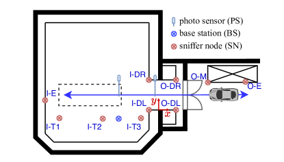
Figure 1: Measurement setup. The Car is driving in and out of the automotive testbed.

TABLE I: Label and position of sniffer-nodes

		Position in m
Label	Description	x	y	z
I-E	inside end	-13.30	0.90	0.64
I-T1	inside top 1	-9.88	-0.35	3.92
I-T2	inside top 2	-6.58	-0.35	3.92
I-T3	inside top 3	-1.60	-0.35	3.92
I-DR	inside door right	-1.55	3.19	1.00
I-DL	inside door left	-1.55	-0.09	1.00
O-E	outside end	11.10	2.02	1.70
O-M	outside mid	6.80	2.32	1.84
O-DR	outside door right	2.21	3.10	0.99
O-DL	outside door left	2.21	0.00	1.00

II-A Hardware and Protocol

We used the BLE physical (PHY) layer and combined it with the Energy and Power Efficient Synchronous Sensor Network (EPhESOS) protocol [9] to realize an IWSN with up to 100 nodes per BS. EPhESOS provides a deterministic media access control (MAC) layer using time division multiple access (TDMA), with a superframe (SF) length of 100 ms. As hardware platform for the measurements and all applications, the Nordic™NRF52840 controller with integrated transceiver is used.

II-B Acquired Dataset

In the course of this work, a large number of measurements were collected, which are published and provided as open-source data set under SAL Autarkic Localization RSSI BLE Dataset (SAL-RB-Dataset) [10]. The acquired data set consists of: (i) two disjoint measurement-sets, where a person walks inside and outside the automotive testbed, and (ii) eight disjoint measurement-sets, where a car is driving in and out the testbed as depicted in Fig. 1. For (ii) two different MN were mounted on the car to investigate the effects of different hardware on the classification. Each individual set provides RSSI values of all ten SN in a 100 ms interval. A missing link is denoted with -100 dBm. The labels of the RSSI values correspond to different localization cells and are defined as follows:

• Label = 0:  car is outside the testbed

• Label = 1:  car is completely inside the testbed

• Label = 2:  car is inside the testbed and on test-position

In total the data set consists of more than 20 000 labeled RSSI measurements for each SN. Figure 2 shows example measurements of the RSSI values in dBm for the SNs $\{\text{I-E, I-DR, O-M, O-DR}\}$ and the corresponding labels.

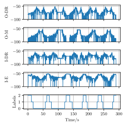
Figure 2: Exemplary RSSI measurements in dBm of four SNs with the corresponding labels.

To evaluate the findings of this work, six car measurement-sets from the SAL-RB-Dataset are used.

III RSSI-based Machine Learning Classifier

The MLC uses the sniffed RSSI values of data packets sent by the MN to identify its position, or more precisely the label of the corresponding cell in the testbed. The RSSI measurements from the ten SNs ($N=10$) are synchronously recorded at time step $t$ and collected in the input vector $\mathbf{x}_{t}\in\mathbb{R}^{N}$ which is used to estimate the corresponding label $y_{t}\in\{0,1,2\}$. As usual, the MLC has an offline training phase and an online classifier phase. The training set $\{\mathbf{x}^{\prime}_{1:T^{\prime}},\,y^{\prime}_{1:T^{\prime}}\}$ with $T^{\prime}$ samples is used to train the classifier. Afterwards the classification is performed online with the measured data to estimate the label $\hat{y}_{t}$. The performance of the classification is assessed by the accuracy score which is calculated as the number of correctly identified labels divided by the number of all classifications.

III-A Machine Learning Methods and Data Splitting

In the following, we focus on simple machine learning techniques to enable the estimator implementation directly at node level. We considered three widely used algorithms, namely K-Nearest Neighbors (KNN), Random Forest (RF), and Support Vector Machine (SVM). All of these algorithms fall into the category of supervised machine learning techniques, where the choice of measurement-sets for the training and subsequent validation is crucial. A common procedure here is to perform a random split of the measurement data to obtain a subset for training and validation. However, since the RSSI values are measured continuously, subsequent measurements tend to be very similar. A random split would lead in this case to a very good, though, unrealistic accuracy score, as the smaller validation set contains nearly identical measurements of the training set. To avoid this, we do not split or shuffle individual measurements set, but keep them whole either for training or testing. This approach is also comparable to the real use-case since here the MLC would also be learned at the beginning and should then work for future measurements. Additionally, instead of using only a single training and validation set, all combinations consisting of three training and one validation data sets, without using the same for both, are evaluated in this section. This ensures a fair comparison of the different MLC since it mitigates the problem that some approaches may be exceptionally good for some data set combinations.

The three proposed algorithms are implemented using Scikit-learn which is an open-source machine learning library for Python [11]. For the given classification task, all three algorithms performed similarly in terms of accuracy and robustness, though the SVM showed slightly higher accuracy. With the RSSI values directly as input, the SVM reached an average accuracy of 77 % for the given data set [10] and is used exclusively for all following evaluations.

The remaining miss-classifications are caused by overlapping class-conditional distributions due to noise and limited dynamic range of the measurements. These mainly occur at class transition regions in the testbed, e.g., the doorstep and test-position, and none of the proposed MLC could improve in these areas. In order to further improve the accuracy, especially at the class boarders, we introduce more suitable input features for the MLC and a subsequent post-processing.

III-B Selecting Features for Machine Learning Classifier

Regarding feature selection, two questions have to be answered. Firstly, it is necessary to know whether the raw data $\mathbf{x}_{t}$ of one SF is sufficient for the classification, or if including previous samples will improve the performance. Secondly, it is essential to validate how the position, number, and combination of the SNs influences the accuracy. In this context, it is important to answer if also a subset of nodes is sufficient for the classification task.

Also for this evaluation, the choice of measurement-sets for the training and subsequent validation is crucial. To ensure a fair comparison of the different features all combinations of three training and one validation data sets, without using the same for both, are evaluated. This mitigates the problem that some features may be exceptionally good for some data set combinations

III-B1 Short-Term Moments as Features

The drawback of using the RSSI measurements of more than one SF as input features is, that it increases the feature space with each additional sample. Besides that, the selected MLC may not be able to model the relation of sequential input data, e.g. RSSI values are considered individually and the dynamic relation over time is not modeled.

To avoid this, we propose to use short-term estimates of the first two moments over $L$ samples. Thus, we introduce

$$\mathbf{x}_{t}^{\mu\sigma}=\Bigg{[}\underbrace{\frac{1}{L}\sum_{\tau=t-L+1}^{t}{x}_{\tau}}_{\bar{x}^{L}_{t}},\quad\underbrace{\frac{1}{L-1}\sum_{\tau=t-L+1}^{t}({x}_{\tau}-\bar{x}^{L}_{t})^{2}}_{s_{t}^{L}}\Bigg{]}\,.$$ (1)

This only doubles the feature space, independently of the number of used SFs. To get an indication of how many preceding samples benefit this approach in our scenario, we consider the coherence time of the channel. The coherence time $T_{c}$ is a statistical measure of the time duration over which two received signals have a certain minimum amplitude correlation, depending on the relative motion between the MN on the car and the SNs. It can be estimated according to [12] with

$$T_{c}=\sqrt{\frac{9}{16\pi f_{m}^{2}}}=\frac{0.423}{f_{m}}\,,$$ (2)

where $f_{m}$ is the Doppler spread, which is upper bounded by the maximum occurring Doppler shift, calculated as $f_{max}=v/\lambda$. With the given BLE center frequency $f_{c}=2.44\,\text{GHz}$ and the average speed of the car $v=1\,\frac{\text{m}}{\text{s}}$, the Doppler shift in case of directly oncoming movement is about 8 Hz, which results in a lower bound of $T_{c}\approx 50\,\text{ms}$. Since the time interval between two successive SFs is 100 ms, considering more than two RSSI measurements for (1) may not improve the result.

To investigate this and to analyze the advantages of using short-term moments as input features, we use the SVM classifier and compare the results for an increasing number $L$ in (1). Figure 3 depicts the accuracy score of the classifier over $L$, where $L=1$ denotes the result using the raw RSSI values. The depicted accuracy is the average accuracy over all $1023$ possible SN-combinations and 60 possible training and validation data set combinations. As mentioned before, this assures a fair comparison since we observed that the short-term moments showed a higher improvement for certain combinations. In contrast to the calculated coherence time, the accuracy further increases with $L$, though the highest relative gain is achieved by using one additional preceding measurement.

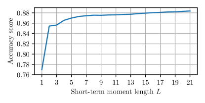
Figure 3: Accuracy score over increasing short-term moment length $L$ for the SVM. The raw RSSI measurements are indicated with $L=1$.

III-B2 Node Selection Scheme

Due to noise and the limited dynamic range of the measurements, two SNs can provide similar RSSI values, though they are at different locations. Additionally, some SN positions may provide exceptional good measurements for the given classification task, since the main effect that is exploited is not the free-space pathloss, but the changes between line-of-sight and non-line-of-sight channel caused by the movement of the car. Not only the positions of the SNs are important, but also the combination of the individual RSSI measurements is crucial for the correct classification. Instead of evaluating all SN combinations and simply choosing the one with the highest accuracy, we first determine combinations that provide poor performance.

Figure 4 depicts the distribution of the accuracy score of all 1023 SN-combinations averaged over all data set combinations using the raw RSSI values and the short-term moments in (1) with $L=2$. Again the advantages of the short-term moments can be observed, as all individual SN-combinations show a higher accuracy. Additionally, they are clustered at higher percentages which indicate improved robustness. Because the short-term moments are superior as input features, in the following we will use them exclusively.

Most SN-combinations show an accuracy between 80-90 %, tending to the higher ones, while only very few combinations are below. On closer inspection of the few combinations that lead to poor results, we found an intuitive explanation. These combinations are composed of either SNs only outside, only inside, or only single SNs. On the contrary, combinations that are composed of SNs equally spaced in the area of interest, including nodes at significant points, e.g. near the doorstep, lead to very good results. We found out that about four SNs are sufficient for our task, with for example the combination $\{\text{I-E, I-DR, O-M, O-DR}\}$.

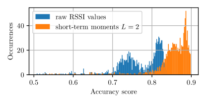
Figure 4: Accuracy score distribution of all SN combinations using the raw RSSI measurements and short-term moments for the SVM.

III-C Refining Cell Estimates Via Post-Processing

The physical cell-boarders in the $x$-dimension, as depicted in Fig. 1 with the PSs, are defined w.r.t. the given localization task and are not chosen optimal in terms of high differences in the measured RSSI values. As a result, noise and limited dynamic range of the RSSI measurements lead to oscillating miss-classifications in time, especially near the physical borders of the cells, i.e. doorstep and test-position. Miss-classifications can also occur in the middle of the cell, e.g. inside the testbed at the far end, which in particular is a problem for the mentioned industrial use-case.

Therefore, we propose a second classification stage to mitigate this problem. Instead of considering SFs individually, we include a certain dynamic in the classification model, because the samples are highly correlated in time. For example preceding measurements have a high probability to result in the same cell and abrupt changes for a few SFs are physically not possible. The two stage-approach consist of, (i) the MLC for the current input vector $\mathbf{x}_{t}$ or $\mathbf{x}_{t}^{\mu\sigma}$ respectively and the corresponding output $\hat{y}_{t}$, and (ii) a filter to account for the dynamic in the cell transitions with the output $\hat{z}_{t}$. For (ii) we propose two approaches, a simple median filter and a filter based on Hidden Markov Models [13].

III-C1 Median Filter

By applying a median filter we mitigate the abrupt changes in the cell estimate. The output of the MLC $\hat{y}_{t}$ at the time step $t$ is filtered using $M$ past predictions with a windowed median filter

$$\hat{z}_{t}=\operatorname{med}\big{(}\hat{y}_{t-M},\dots,\hat{y}_{t}\big{)}\,,$$ (3)

where $\hat{y}_{t}\in\{0,1,2\}$. The median filter is only able to improve the classification if the first stage already provides a sufficiently good result with only a few errors. It also does not account for the probabilities of the individual cell transitions or whether these cell transitions are even possible, e.g. a change from $0$ to $2$ and vice versa is not possible in our scenario.

III-C2 Hidden Markov Model

Here, we assume that the observed cell estimates are corrupted versions of the true cell positions and impose probabilities both for the cell transitions, as well as for corrupt observations. This allows us to define a model for the cell transitions instead of the purely empirical median filter approach. To limit the complexity of the post-processing, we assume that the Markov property is satisfied, that is, the cell or label at time $t+1$ is conditionally independent on the past, given the current cell estimate at time $t$, or

$$p\big{(}z_{t+1}|z_{t},z_{t-1},\dots\big{)}=p\big{(}z_{t+1}|z_{t}\big{)}\,,$$ (4)

with $z_{t}\in\{S^{1},S^{2},\dots,S^{n}\}$. $S^{i}$ refers to the $i$th possible true cell location. In our case, we observe the original cells, but with possible flips between true and observed cells, hence $y_{t}\in\{S^{1},S^{2},\dots,S^{n}\}$ holds as well. We use a HMM with $n=3$ hidden states which is defined by

• the transition matrix $\mathbf{A}\in\mathbb{R}^{n\times n}$ with the probabilities $a_{ij}=p\big{(}z_{t+1}=S^{j}|z_{t}=S^{i}\big{)}$ of transition from state $S^{i}$ to state $S^{j}$,

• the emission matrix $\mathbf{B}\in\mathbb{R}^{n\times n}$ with the probabilities $b_{ij}=p\big{(}\hat{y}_{t}=S^{j}|z_{t}=S^{i}\big{)}$ to observe $\hat{y}_{t}=S^{j}$ in the state $S^{i}$, and

• the state probability vector $\boldsymbol{\pi}_{t}\in\mathbb{R}^{n}$  with the probabilities $\pi_{t,i}=p\big{(}z_{t}=S^{i}\big{)}$ that $S^{i}$ is the cell location at time $t$. $\boldsymbol{\pi}_{0}$ denotes the initial state.

The HMM takes the sequence of estimates $\hat{y}_{t}$ of the MLC as observations and returns a sequence of cell estimates $\hat{z}_{t}$ as output. The finding of suitable parameters $\mathbf{A}$, $\mathbf{B}$ and $\boldsymbol{\pi}_{0}$ is also referred to as learning problem. Since the HMM should correct the miss-classified samples, an intuitive approach is to use the mistakes from the MLC in the training phase, i.e. calculate the transition and emission matrix with the training data $\{\mathbf{x}^{\prime}_{1:T^{\prime}},y^{\prime}_{1:T^{\prime}}\}$ and the corresponding prediction $\hat{y}^{\prime}_{1:T^{\prime}}$. The transition matrix $\mathbf{A}$ describes the probability of each state transition, hence, we estimate the entries with the labels of the training data $y^{\prime}_{1:T^{\prime}}$ according to

$$\hat{a}_{ij}=\frac{\sum_{t=1}^{T^{\prime}-1}\delta[y^{\prime}_{t},S^{i}]\delta[y^{\prime}_{t+1},S^{j}]}{\sum_{t=1}^{T^{\prime}}\delta[y^{\prime}_{t},S^{i}]}\,,$$ (5)

where $\delta[a,b]$ is the Kronecker delta function which equals 1 for $a=b$ and 0 otherwise. For the estimation of the emission matrix $\mathbf{B}$, we use the confusion matrix $\mathbf{C}$ of the predicted labels $\hat{y}^{\prime}_{1:T^{\prime}}$, where the entry $c_{ij}$ represents the number of samples where the original label of the training data is $S^{i}$, but $S^{j}$ was predicted. Since the entries of the emission matrix define the probabilities of a cell depending on an observation, we can directly use the normalized confusion matrix for the estimation with

$$\hat{b}_{ij}=\frac{c_{ji}}{\sum_{i=1}^{n}c_{ji}}\,.$$ (6)

For the choice of the initial vector $\boldsymbol{\pi}_{0}$ we have two options assuming the initial state is unknown: (i) calculate the probability of each cell by counting the occurrences in the training data $y^{\prime}_{i:T^{\prime}}$ or (ii) assume an uninformative prior, where each state has the same probability. In this work, the more general case (ii) is chosen and the entries of the initial vector are estimated by

$$\hat{\pi}_{0,i}=\frac{1}{n}\,,$$ (7)

where $n$ is again the number of states.

In the so-called decoding problem, the learned HMM is used to find the most likely state sequence $\hat{z}_{1:T}$ of the model that produced the observation $\hat{y}_{1:T}$. This problem is usually solved using the Viterbi algorithm with the drawback that it needs a sequence of observations for the prediction. In this work, a simple forward approach is used to perform cell predictions in online fashion using the forward algorithm. The forward algorithm calculates the state probabilities $\boldsymbol{\pi}_{t}$ at a certain time step $t$ using the previous state probability and the current observation. The algorithm is initialized with $\boldsymbol{\pi}_{1}=\boldsymbol{\pi}_{0}\circ\left(\mathbf{e}_{y_{1}}\mathbf{B}\right)$, where $\mathbf{e}_{n}$ is the canonical basis row vector with $1$ in the $n$th element and $0$ otherwise. For each following observation the state probability is calculated with

$$\boldsymbol{\pi}_{t}=\left(\frac{\boldsymbol{\pi}_{t-1}\mathbf{A}}{\sum_{i=1}^{n}\pi_{t-1,i}}\right)\circ\left(\mathbf{e}_{y_{t}}\mathbf{B}\right)\,.$$ (8)

The estimation of the cell $\hat{z}_{t}$ is given by the state with highest probability in $\boldsymbol{\pi}_{t}$.

IV Classifier Evaluation

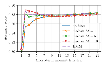
Figure 5: Accuracy score over increasing short-term moment length $L$ with and without additional filtering for the SVM

Both proposed post-processing approaches are compared using the average accuracy score similar to Section III-B1 and the results are depicted in Fig. 5 for increasing $L$ in (1). For the median filter three different window lengths $M=\{1,5,10\}$ are considered. It can be observed that both approaches are able to improve the accuracy of the classification. In contrast to the raw output of the MLC, the accuracy does not improve with increasing $L$ after the proposed filtering. The highest accuracy is achieved in both cases for $L=2$, which matches the fact that more than $2$ samples significantly oversteps our calculated coherence time estimate.

Although the median filter shows slightly better results for a sufficient window length, the HMM is favourable since it can be adapted easily to various other classification problems and for (8) only the state probability of the preceding sample is needed. The median filter requires storing more previous predictions and the accuracy does not necessarily improve with increasing window lengths. It only smooths the output of the classifier by preventing abrupt cell changes, however, this might not be suitable for all applications.

In the following, the classification is performed with the SN combination $\{\text{I-E, I-DR, O-M, O-DR}\}$ and a single data set combination. Figure 6 depicts the results of the MLC for: (a) the raw RSSI measurements with an accuracy of 86.2 %, and (b) the short-term moments with $L=2$ and an additional HMM filtering with an accuracy of 93.5 %. Note that in contrast to Fig. 3, the accuracy is higher since here an adequate SN combination was chosen.

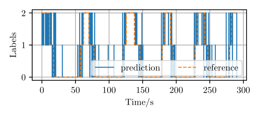
(a) raw RSSI measurements

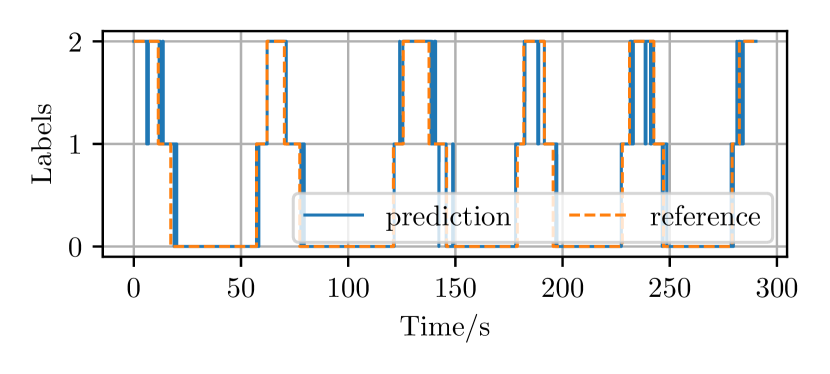
(b) short-term moments $L=2$ and HMM

Figure 6: Predicted labels compared to ground truth reference using the SN combination $\{\text{I-E, I-DR, O-M, O-DR}\}$ using the SVM as MLC

V Conclusion

We analyzed the performance of cell-level localization based on RSSI values, measured in an already existing IWSN. The evaluation showed that for this task the accuracy of the used MLC was comparable to each other, while the choice of good data pre- and post-processing was the key to higher accuracy. The introduced features based on short-term moments significantly increased the accuracy and robustness of the MLC by considering only one preceding RSSI measurement. To mitigate abrupt changes of the estimate at the output of the MLC we added an additional classification stage. Here the HMM showed excellent cell-level localization results with an accuracy of $93.5\,\%$. Due to the learning based on the confusion matrix and training data, it can be adapted to various other classification problems. Based on an extensive measurement campaign we were able to test the algorithms in detail and also investigate the importance of SN position and combination. The proposed approach can be easily implemented at node-level to directly label the measurements or verify them based on their location.

References

- [1] A. A. Kumar S., K. Ovsthus, and L. M. Kristensen., “An Industrial Perspective on Wireless Sensor Networks — A Survey of Requirements, Protocols, and Challenges,” IEEE Communications Surveys Tutorials, vol. 16, no. 3, pp. 1391–1412, 2014.
- [2] K. Montgomery, R. Candell, Y. Liu, and M. Hany, “Wireless user requirements for the factory workcell,” Tech. Rep., National Institute of Standards and Technology, jan 2020.
- [3] S. Raza, M. Faheem, and M. Guenes, “Industrial wireless sensor and actuator networks in industry 4.0: Exploring requirements, protocols, and challenges—A MAC survey,” International Journal of Communication Systems, vol. 32, no. 15, pp. e4074, 2019.
- [4] H.-P. Bernhard, J. Karoliny, B. Etzlinger, and A. Springer, “Work-in-progress: Rssi-based presence detection in industrial wireless sensor networks,” in 2020 16th IEEE International Conference on Factory Communication Systems (WFCS), 2020, pp. 1–4.
- [5] European Commission., “Commission regulation (eu) no 459/2012 of 29 may 2012 amending regulation (ec) no 715/2007 of the european parliament and of the council and commission regulation (ec) no 692/2008 as regards emissions from light passenger and commercial vehicles (euro 6)(1),” Off. J. Eur. Union, L: Legis., vol. 55, pp. 16–24, 2012.
- [6] H. Liu, H. Darabi, P. Banerjee, and J. Liu, “Survey of Wireless Indoor Positioning Techniques and Systems,” IEEE Transactions on Systems, Man, and Cybernetics, Part C (Applications and Reviews), vol. 37, no. 6, pp. 1067–1080, 2007.
- [7] K. Lee and L. Lampe, “Indoor cell-level localization based on RSSI classification,” in 2011 24th Canadian Conference on Electrical and Computer Engineering(CCECE), 2011, pp. 000021–000026.
- [8] S. Mahfouz, P. Nader, and P. E. Abi-Char, “RSSI-based classification for indoor localization in wireless sensor networks,” in 2020 IEEE International Conference on Informatics, IoT, and Enabling Technologies (ICIoT), 2020, pp. 323–328.
- [9] H. Bernhard, A. Springer, A. Berger, and P. Priller, “Life cycle of wireless sensor nodes in industrial environments,” in 2017 IEEE 13th International Workshop on Factory Communication Systems (WFCS), 2017, pp. 1–9.
- [10] J. Karoliny, T. Blazek, F. Ademaj, and H. Bernhard, “SAL-Autarkic-Localization-RSSI-BLE-Dataset: SAL- RB-Dataset,” Distributed by Zenodo https://doi.org/10.5281/zenodo.4073072, Oct. 2020.
- [11] F. Pedregosa, G. Varoquaux, A. Gramfort, V. Michel, B. Thirion, O. Grisel, M. Blondel, P. Prettenhofer, R. Weiss, V. Dubourg, J. Vanderplas, A. Passos, D. Cournapeau, M. Brucher, M. Perrot, and E. Duchesnay, “Scikit-learn: Machine learning in Python,” Journal of Machine Learning Research, vol. 12, pp. 2825–2830, 2011.
- [12] T. S. Rappaport et al., Wireless communications: principles and practice, vol. 2, prentice hall PTR New Jersey, 1996.
- [13] B. Esmael, A. Arnaout, R. K. Fruhwirth, and G. Thonhauser, “Improving time series classification using hidden markov models,” in 2012 12th International Conference on Hybrid Intelligent Systems (HIS), 2012, pp. 502–507.