Supersymmetric solitons and a degeneracy of solutions in AdS/CFT

Abstract

We study Lorentzian supersymmetric configurations in $D=4$ and $D=5$ gauged $\mathcal{N}=2$ supergravity. We show that there are smooth $1/2$ BPS solutions which are asymptotically AdS₄ and AdS₅ with a planar boundary, a compact spacelike direction and with a Wilson line on that circle. There are solitons where the $S^{1}$ shrinks smoothly to zero in the interior, with a magnetic flux through the circle determined by the Wilson line, which are AdS analogues of the Melvin fluxtube. There is also a solution with a constant gauge field, which is pure AdS. Both solutions preserve half of the supersymmetries at a special value of the Wilson line. There is a phase transition between these two saddle-points as a function of the Wilson line precisely at the supersymmetric point. Thus, the supersymmetric solutions are degenerate, at least at the supergravity level. We extend this discussion to one of the Romans solutions in four dimensions when the Euclidean boundary is $S^{1}\times\Sigma_{g}$ where $\Sigma_{g}$ is a Riemann surface with genus $g>0$. We speculate that the supersymmetric state of the CFT on the boundary is dual to a superposition of the two degenerate geometries.

1 Introduction

There is a long-standing interest in smooth soliton solutions in gravity. There are many examples where some $S^{1}$ direction shrinks smoothly to zero, starting with the bubble of nothing instability of the Kaluza-Klein vacuum [1]. A similar solution with asymptotically locally AdS boundary conditions was dubbed the AdS soliton [2]. These solutions are easily constructed; they are simply double analytic continuations of black hole solutions (in these examples, uncharged black holes in asymptotically flat or asymptotically AdS space). In the AdS case, the soliton is a time-independent solution, with a flat conformal boundary. The spin structure of a spacetime with a contractible $S^{1}$ has antiperiodic boundary conditions on the $S^{1}$. In the holographic AdS/CFT correspondence, the dual theory thus has a spatial circle with antiperiodic boundary conditions for fermions; if the CFT was supersymmetric this choice of boundary conditions breaks the supersymmetry. The AdS soliton is dual to the ground state in this theory. It has a negative energy, which is identified with the Casimir energy of the dual CFT; the antiperiodic boundary conditions for fermions spoil the cancellation between the bosons and fermions.

A simple generalization of these boundary conditions in the CFT is to add a Wilson line around the non-trivial cycle, giving a non-trivial holonomy for the bulk gauge field. A family of bulk solutions satisfying these boundary conditions can be obtained by a double analytic continuation of electrically charged black holes. After the analytic continuation, the solutions have a magnetic flux through the circle; in the bulk the Wilson line is related to the total amount of magnetic flux through this cycle. These are AdS analogues of the Melvin fluxtube solutions in flat space [3], and were previously studied in [4, 5, 6]. For simplicity, we study the solutions primarily in four bulk dimensions with a flat boundary, but we also consider generalisations in Euclidean signature to a boundary which is $S^{1}\times\Sigma_{g}$ for some Riemann surface of genus $g>1$, and to five bulk dimensions, which may be interesting for its relation to $\mathcal{N}=4$ SYM.

Surprisingly, there is a solution of vanishing energy in this family which is supersymmetric. This is surprising, as the solutions still have the same structure as the AdS soliton, with a smooth origin which enforces antiperiodic boundary conditions for the fermions on the shrinking $S^{1}$, which we normally think of as breaking the supersymmetry. However, the holonomy around the circle can compensate for the change in boundary conditions. The supersymmetry of these solutions has been recognised in various guises before. They are double analytic continuations of a set of supersymmetric naked singularities identified in four dimensions in [7, 8] and in five dimensions in [9]. They were also studied in four dimensional Euclidean space very recently in [10] as an extension of the supersymmetric black holes dual to the twisted supersymmetric index. We add to these previous discussions by emphasizing the previously unnoticed fact that these solutions are perfectly well behaved Lorentzian configurations. Indeed, these configurations can be thought as a supersymmetric extension of the AdS soliton of [2]. We provide a detailed discussion of the role of its spin structure; we will explicitly construct the antiperiodic Killing spinors in the bulk spacetime.

In addition to these smooth soliton solutions, there are also solutions with these boundary conditions where the $S^{1}$ does not have a smooth origin in the bulk. In the simple case with flat boundary conditions, this solution is simply AdS in Poincaré coordinates, with one of the spatial directions identified. For $S^{1}\times\Sigma_{g}$ boundary conditions, the solution is an analytic continuation of the magnetically charged black hole solution of Romans, with an AdS${}_{2}\times\Sigma_{g}$ near-horizon region [7, 11, 12]. A solution with a Wilson line is easily obtained by adding a constant gauge potential in the bulk, without changing the geometry. These solutions are supersymmetric for integer-quantized values of the Wilson line, with periodic Killing spinors for even $n$ and antiperiodic Killing spinors for odd $n$.

Thus, for a range of values of the Wilson line on the $S^{1}$, there are two bulk solutions with these boundary conditions: the magnetic flux tube solution and the solution dressed with a constant gauge field. We will show that there is a phase transition between these two families of solutions precisely at the supersymmetric point with antiperiodic Killing spinors; the ground state of the CFT with these boundary conditions is the soliton for smaller values of the Wilson line, and the constant gauge field solution for larger values.

The path integral for the CFT on an $S^{1}\times\Sigma_{g}$ with the supersymmetry-preserving choice of Wilson line computes the twisted supersymmetric index [13, 14, 15]. In this context, both of these three-dimensional configurations have been considered before: the solution with the constant gauge field was studied in [12] as the bulk dual of this twisted partition function. It was noted in [10] that there is a supersymmetric solution with an $\mathbb{R}^{2}\times\Sigma_{g}$ near-horizon region; our magnetic flux tube. However, it was not previously appreciated that these solutions compete.

This is as far as we know the first example where there is a degeneracy between bulk solutions in a supersymmetric partition function, and it would be fascinating to understand its implications for the field theory. It would be interesting to study the one-loop determinant of the bulk fields on both solutions to see if this lifts the degeneracy. We conjecture that it does not, and the supersymmetric ground state in field theory is dual to a superposition of the two geometries. If so, this would be the first example we know where a field theory ground state has such an interpretation. It would then be very interesting to consider the observables in this state, such as correlation functions, whose calculation in the bulk will be sensitive to the relative phase between the two solutions. It is also interesting that there is qualitative difference between even and odd integer-quantized Wilson lines; in the even case, with periodic Killing spinors, there is a unique supersymmetric solution in the bulk, while in the odd case there is this degeneracy.

In the first part of the paper, we will discuss the case with flat boundary in AdS₄ in some detail. We set up the bulk theory in section 2.1, and describe the solutions in section 2.2. We give a careful analysis of supersymmetry in section 2.3, and describe the phase structure in section 2.4. We then briefly discuss the extension to $S^{1}\times\Sigma_{g}$ boundaries in section 3. We generalize the analysis to AdS₅ for flat boundaries in section 4.

2 Four dimensions

2.1 Gauged $\mathcal{N}=2$ supergravity

Our explicit discussion of solutions in four dimensions is carried out in the context of minimal gauged $\mathcal{N}=2$ supergravity in four dimensions. This theory was originally constructed in terms of the physical fields [17, 18], whose supersymmetry transformations only close under commutation up to equations of motion. Subsequently two alternative constructions were presented based on the superconformal multiplet calculus [19, 20, 21]. This theory is a universal subsector of a range of four-dimensional supersymmetric theories. The bosonic sector is the familiar Einstein-Maxwell-AdS theory, with action

$$S\left(g,A\right)=\int d^{4}x\sqrt{-g}\left[\frac{R}{2}-\frac{1}{8}F_{\mu\nu}F^{\mu\nu}+\frac{3}{\ell^{2}}\right],$$ (1)

where $F(A)_{\mu\nu}=\partial_{\mu}A_{\nu}-\partial_{\nu}A_{\mu}\,.$The field equations are

$$\partial_{\mu}\big{(}\sqrt{-g}F^{\mu\nu}\big{)}=0\,\,,$$

$$R_{\mu\nu}-\tfrac{1}{2}g_{\mu\nu}R-\tfrac{1}{2}\big{[}F_{\mu\rho}\,F_{\nu}{}^{\rho}-\tfrac{1}{4}g_{\mu\nu}F_{\rho\sigma}F^{\rho\sigma}\big{]}-\frac{3}{\ell^{2}}\,g_{\mu\nu}=0\,.$$ (2)

When supplemented by the fermionic sector, the supergravity theory is invariant under supersymmetry transformations of all the fields. In our calculations we will only make use of the transformation of the chiral Rarita-Schwinger fields $\psi_{\mu}{\!}^{i}\,$:

$$\delta\psi_{\mu}{\!}^{i}=\; 2\,\mathcal{D}_{\mu}\epsilon^{i}-\tfrac{1}{4}F(A)_{\rho\sigma}\gamma^{\rho\sigma}\gamma_{\mu}\,\varepsilon^{ij}\,\epsilon_{j}+\ell^{-1}\,\varepsilon^{ij}\,t_{j}{}^{k}\,\gamma_{\mu}\epsilon_{k}\,,$$ (3)

$$\delta\psi_{\mu\,i}=\; 2\,\mathcal{D}_{\mu}\epsilon_{i}-\tfrac{1}{4}F(A)_{\rho\sigma}\gamma^{\rho\sigma}\gamma_{\mu}\,\varepsilon_{ij}\,\epsilon^{j}+\ell^{-1}\,\varepsilon_{ij}\,t^{j}{}_{k}\,\gamma_{\mu}\epsilon^{k}\,,$$ (4)

where $\gamma^{5}=-\mathrm{i}\gamma^{0}\gamma^{1}\gamma^{2}\gamma^{3}$, $\gamma^{5}\psi_{\mu}^{i}=\psi_{\mu}^{i}$ and $\gamma^{5}\psi_{\mu i}=-\psi_{\mu i}$ and $i=1,2$ and we shall pick $t^{i}{}_{j}=$ $\mathrm{i}\sigma_{3}\Longrightarrow t_{i}{}^{j}=$ $-\mathrm{i}\sigma_{3}$. The covariant derivatives of the supersymmetry parameters are given by

$$\mathcal{D}_{\mu}\epsilon^{i}= \;\big{(}\partial_{\mu}+\tfrac{1}{4}\omega_{\mu}{\!}^{ab}\gamma_{ab}\big{)}\epsilon^{i}-\tfrac{1}{2\ell}A_{\mu}\,t^{i}{\!}_{j}\,\epsilon^{j}\,,$$ (5)

$$\mathcal{D}_{\mu}\epsilon_{i}= \;\big{(}\partial_{\mu}+\tfrac{1}{4}\omega_{\mu}{\!}^{ab}\gamma_{ab}\big{)}\epsilon_{i}-\tfrac{1}{2\ell}A_{\mu}\,t_{i}{}^{j}\,\epsilon_{j}\,.$$ (6)

In our calculations we find that is convenient to work with the spinor

$$\chi\equiv\epsilon^{1}+\epsilon_{2}\,,$$ (7)

such that the Killing spinor equation is

$$2\,\mathcal{D}_{\mu}\chi+\tfrac{1}{4}F(A)_{\rho\sigma}\gamma^{\rho\sigma}\gamma_{\mu}\gamma^{5}\,\chi-\ell^{-1}\mathrm{i}\,\gamma_{\mu}\gamma^{5}\chi=0\,,$$ (8)

where the covariant derivative of $\chi$ follows from (5),

$$\mathcal{D}_{\mu}\chi=\big{(}\partial_{\mu}+\tfrac{1}{4}\omega_{\mu}{\!}^{ab}\gamma_{ab}-\tfrac{1}{2\ell}\,\mathrm{i}\,A_{\mu}\big{)}\chi\,.$$ (9)

We recall that all fermionic fields have been suppressed on the right-hand side of equation (9), because we will be dealing with purely bosonic backgrounds. In the following sections we will consider a class of soliton solutions that can be partially supersymmetric. Their possible supersymmetry will be investigated by analyzing the equation (8).

The Lagrangian (1) can be obtained from the compactification of eleven dimensional supergravity over the seven sphere with the ansatz [22]

$$ds_{11}^{2} =ds_{4}^{2}+4\ell^{2}\sum_{i}\left(d\mu_{i}^{2}+\mu_{i}^{2}\left(d\phi_{i}+\frac{1}{4\ell}A\right)^{2}\right).$$ (10)

$$F_{4} =-\frac{3}{\ell}\epsilon_{4}-2\ell^{2}\sum_{i}\mu_{i}d\mu_{i}\wedge\left(d\phi_{i}+\frac{1}{4\ell}A\right)\wedge\ast_{4}dA$$ (11)

where $\ast_{4}$ is the Hodge dual with respect to the four-dimensional metric $ds_{4}^{2}$ and $\epsilon_{4}$ its volume form. The $\phi_{i}$ are $2\pi$ periodic angular coordinates parametrizing the four independent rotations on $S^{7}$. We will be interested in considering the higher-dimensional interpretation of some of our solutions using this uplift.

2.2 Planar solitons

The solutions we consider all have metric

$$ds^{2}=\frac{r^{2}}{\ell^{2}}\left(-dt^{2}+dz^{2}\right)+\frac{dr^{2}}{f(r)}+f(r)d\phi^{2}\,.$$ (12)

When considering supersymmetry we will also need a corresponding set of vierbeine, which we take to be

$$e^{0} =\frac{r}{\ell}dt\,,$$

$$e^{1} =\frac{\,dr}{\sqrt{f(r)}}\,,$$

$$e^{2} =\sqrt{f(r)}d\phi\,,$$

$$e^{3} =\frac{r}{\ell}dz.$$ (13)

The simplest solution has

$$f(r)=\frac{r^{2}}{\ell^{2}}\,.$$ (14)

If $\phi$ is not periodically identified, this is simply pure $\mathrm{AdS}_{4}$ in Poincaré coordinates. However, we are interested in considering solutions with $\phi$ periodically identified in the boundary. For Poincaré-AdS, we can impose this identification on the bulk as a quotient. We will postpone a full discussion of this quotient until we have discussed the soliton solution.

The soliton solution is

$$f(r) =\frac{r^{2}}{\ell^{2}}-\frac{\mu}{r}-\frac{Q^{2}}{r^{2}}\,,$$ (15)

$$A =\left(\frac{2Q}{r}-\frac{2Q}{r_{0}}\right)d\phi\text{ ,}$$ (16)

where $r_{0}$ is the largest root of the equation $f(r_{0})=0$. This solution can be obtained by a double analytic continuation from an electrically charged black hole solution, where the analytic continuation also involves analytically continuing the charge $Q$. We have $r\in\left[r_{0},\infty\right)$, and regularity of the metric at $r=r_{0}$ requires that $\phi$ is periodic with period

$$\Delta\phi=\frac{4\pi\ell^{2}r_{0}^{3}}{3r_{0}^{4}+Q^{2}\ell^{2}}.$$ (17)

We have added a constant contribution to the gauge potential to ensure regularity at $r=r_{0}$; there is then a non-trivial holonomy of the gauge field at infinity. This is related to the net magnetic flux along the $z$ axis,

$$\Phi=-\oint A_{\phi}\left(r=\infty\right)d\phi=-\frac{1}{2}\int F_{\mu\nu}dx^{\mu}\wedge dx^{\nu}=\frac{2Q}{r_{0}}\Delta\phi.$$ (18)

The soliton solution is determined by two parameters; from the bulk perspective the natural parametrization is $\mu,Q$ or $r_{0},Q$. From the boundary perspective, the natural parameters are $\Delta\phi,\Phi$. In the usual holographic dictionary, we fix the boundary geometry and the boundary value of $A_{\mu}$, which is interpreted as a background gauge field coupled to a global $U(1)$ symmetry of the CFT. Recall that as discussed in the introduction, for the soliton solutions the bulk spin structure is antiperiodic on the $\phi$ circle, as this contracts smoothly in the interior.

Thus, we consider the CFT on a background

$$ds_{Boundary}^{2}=-dt^{2}+dz^{2}+d\phi^{2},$$ (19)

with $\phi$ taken to be periodic with period $\Delta\phi$, and an antiperiodic spin structure for the fermions, and a Wilson line (holonomy) on the $\phi$ circle with value $\Phi$, and we look for bulk solutions satisfying these boundary conditions. We obtain a suitable bulk soliton solution by solving for $\mu,Q$ as functions of $\Delta\phi,\Phi$. We have

$$\mu=\frac{r_{0}^{4}-Q^{2}\ell^{2}}{r_{0}\ell^{2}},\quad Q=\frac{\Phi r_{0}}{2\Delta\phi},$$ (20)

and inverting (17) gives [6]

$$r_{0}=\frac{2\pi\ell^{2}}{3\Delta\phi}\left(1\pm\sqrt{1-\frac{\Phi^{2}}{\Phi_{max}^{2}}}\right),$$ (21)

where $\Phi_{max}=\frac{4\pi}{\sqrt{3}}\ell$. We see that there are two solutions for $r_{0}$ for $\Phi\in[0,\Phi_{max}]$. At $\Phi=0$, the minus branch has $r_{0}=0$, giving $\mu=Q=0$, so it reduces to the Poincaré-AdS solution. The plus branch has $Q=0$, and

$$\mu=\left(\frac{4\pi\ell}{3\Delta\phi}\right)^{3}\ell,$$ (22)

which is just the AdS soliton. The two branches coalesce at $\Phi=\Phi_{max}$.

The parameters $\mu,Q$ control the subleading parts of the metric and gauge field asymptotically, so they can be interpreted as vevs of the corresponding operators in the field theory. The gauge field gives a vev for the current in the boundary theory,

$$\langle J_{\phi}\rangle=2Q,$$ (23)

and the metric gives a vev for the stress tensor,

$$\left\langle T_{tt}\right\rangle=-\frac{\mu}{2\ell^{2}}\text{ },\qquad\left\langle T_{zz}\right\rangle=\frac{\mu}{2\ell^{2}}\text{ },\qquad\left\langle T_{\phi\phi}\right\rangle=-\frac{\mu}{\ell^{2}}\text{ }.$$ (24)

We see that the energy density of the soliton solutions is negative when $\mu$ is positive. We can write explicitly [6]

$$\left\langle T_{tt}\right\rangle=-\left(\frac{4\pi\ell}{3\Delta\phi}\right)^{3}\frac{1}{4\ell}\left[1-\frac{3\Phi^{2}}{2\Phi_{max}^{2}}\pm\left(1-\frac{\Phi^{2}}{\Phi_{max}^{2}}\right)^{3/2}\right].$$ (25)

We see that the minus branch always has $\left\langle T_{tt}\right\rangle\geq 0$, and the plus branch has $\left\langle T_{tt}\right\rangle<0$ for $\Phi\in[0,\Phi_{S})$, where

$$\Phi_{S}=\frac{\sqrt{3}}{2}\Phi_{max}=2\pi\ell.$$ (26)

In addition to the soliton solutions, another solution with these boundary conditions is simply to take the Poincaré-AdS solution, with a constant gauge field $A=-\frac{2Q}{r_{0}}d\phi$. If $\phi$ were not periodic, this is just pure AdS in Poincaré coordinates, and the gauge field is pure gauge. Taking $\phi$ to be periodic with period $\Delta\phi$, the gauge field has a constant Wilson loop $\Phi=-\frac{2Q}{r_{0}}\Delta\phi$ for all $r$, which can’t be set to zero by a gauge transformation.

It is useful to think of this solution as a quotient of AdS${}_{4}\times S^{7}$. For $\Phi=0$, the quotient has fixed points at $r=0$, so this is not a smooth solution. Furthermore, for the antiperiodic boundary conditions we consider, this solution is unstable as a solution of string theory, as a string wrapped around the $\phi$ circle will become tachyonic for sufficiently small $r$. This solution decays by tachyon condensation, whose likely endpoint is the AdS soliton [23, 24].

However, for $\Phi\neq 0$, the identification involves a shift of the angular coordinates on the sphere. The solution with a constant gauge field uplifts as in (10). Since the gauge potential is constant, if $\phi$ is not periodically identified we can eliminate the gauge field by coordinate redefinitions $\tilde{\phi}_{i}=\phi_{i}+\frac{A_{\phi}}{4\ell}\phi$. The periodic identification of $\phi$ at fixed $\phi_{i}$ then acts as $(\phi,\tilde{\phi}_{i})\sim(\phi+\Delta\phi,\tilde{\phi}_{i}+\Phi/4\ell)$. This is now a smooth quotient, with no fixed points, and the circle in the higher-dimensional space has a minimum size $\Phi/8$, so for $\Phi$ larger than the string scale the tachyon is lifted, and this is a physical solution. It is then interesting to compare this solution to the soliton. We will discuss the phase structure in section 2.4, but we first discuss in more detail the supersymmetric solutions at the special value $\Phi=\Phi_{S}$.

2.3 Supersymmetric solutions

The configuration with zero energy, $\mu=0$, which occurs on the plus branch of solitons at $\Phi=\Phi_{S}=2\pi\ell$, is supersymmetric. At this value of $\Phi$, the Poincaré-AdS solution is also supersymmetric. The supersymmetry of the soliton in the Euclidean section has been noted before [10], but we give a slightly more careful analysis taking into account the antiperiodic boundary conditions for the fermions on the $\phi$ circle. Our remark is that the supersymmetric soliton solutions are perfectly well behaved in the Lorentzian section. We will explicitly exhibit the Killing spinors for this solution, and see how they arise from the higher-dimensional perspective.

For the solitons with $\mu=0$, we can write $r_{0}\vskip 12.0pt plus 4.0pt minus 4.0pt=\sqrt{\ell\left|Q\right|}$. The form of the solution can be simplified by a coordinate transformation

$$r=r_{0}\vskip 12.0pt plus 4.0pt minus 4.0pt\sqrt{\cosh(\rho)},$$ (27)

where the configuration reads

$$ds^{2}=\frac{\ell^{2}}{4}d\rho^{2}+\frac{|Q|}{\ell}\left[\cosh\left(\rho\right)\left(-dt^{2}+dz^{2}\right)+\frac{\sinh\left(\rho\right)^{2}}{\cosh(\rho)}d\phi^{2}\right],$$ (28)

$$A=\frac{2Q}{r_{0}}\left(\frac{1}{\sqrt{\cosh\rho}}-1\right)d\phi.$$ (29)

We use a Majorana basis for the Clifford algebra

$$\gamma^{0}=-\mathrm{i}\left(\begin{array}[c]{cc}0&\sigma_{2}\\ \sigma_{2}&0\end{array}\right),\quad\gamma^{1}=-\left(\begin{array}[c]{cc}\sigma_{3}&0\\ 0&\sigma_{3}\end{array}\right),\quad\gamma^{2}=\mathrm{i}\left(\begin{array}[c]{cc}0&-\sigma_{2}\\ \sigma_{2}&0\end{array}\right),\quad\gamma^{3}=\left(\begin{array}[c]{cc}\sigma_{1}&0\\ 0&\sigma_{1}\end{array}\right).$$ (30)

There are two independent solutions to the Killing spinor equation on this background:

$$\chi_{1}=\frac{\exp\left(-\mathrm{i}\pi\frac{\phi}{\Delta\phi}\right)}{\cosh\left(\rho\right)^{1/4}}\left(\begin{array}[c]{c}\sinh\frac{\rho}{2}\\ -\cosh\frac{\rho}{2}\\ \mathrm{i}\cosh\frac{\rho}{2}\\ \mathrm{i}\sinh\frac{\rho}{2}\end{array}\right),$$ (31)

$$\chi_{2}=\frac{\exp\left(-\mathrm{i}\pi\frac{\phi}{\Delta\phi}\right)}{\cosh\left(\rho\right)^{1/4}}\left(\begin{array}[c]{c}-\cosh\frac{\rho}{2}\\ \sinh\frac{\rho}{2}\\ \mathrm{i}\sinh\frac{\rho}{2}\\ \mathrm{i}\cosh\frac{\rho}{2}\end{array}\right).$$ (32)

The two spinors $\chi_{1}$ and $\chi_{2}$, can be projected over four chiral spinors and therefore the soliton solution is 1/2 BPS. They close on the following Killing vectors:

$$\chi_{2}^{\dagger}\gamma^{0}\gamma^{\mu}\chi_{2}\partial_{\mu}=\chi_{1}^{\dagger}\gamma^{0}\gamma^{\mu}\chi_{1}\partial_{\mu}=\frac{2\ell}{r_{0}}\partial_{t},$$ (33)

$$\chi_{1}^{\dagger}\gamma^{0}\gamma^{\mu}\chi_{2}\partial_{\mu}=-\frac{2\ell}{r_{0}}\left(\partial_{\phi}+\mathrm{i}\partial_{z}\right)\text{ }.$$

There is still the issue that the spinors $\chi_{1}$ and $\chi_{2}$ seem to be ill-defined at $\rho=0$, as they have an explicit dependence on $\phi$, however this dependence corresponds exactly to the form of the Killing spinors of Minkowski in cylindrical coordinates:

$$\left.\chi_{1}\right|_{\rho=0}=\exp\left(-\mathrm{i}\pi\frac{\phi}{\Delta\phi}\right)\left(\begin{array}[c]{c}0\\ -1\\ \mathrm{i}\\ 0\end{array}\right),$$ (34)

$$\chi_{2}=\exp\left(-\mathrm{i}\pi\frac{\phi}{\Delta\phi}\right)\left(\begin{array}[c]{c}-1\\ 0\\ 0\\ \mathrm{i}\end{array}\right).$$ (35)

Hence, our Killing spinors interpolate smoothly between half of the Killing spinors of Minkowski and half of the Killing spinors of AdS₄. Indeed, we see that we have solutions of the Killing spinor equation with non-trivial dependence on $\phi$, whereas we would normally expect the Killing spinors to be constant along these flat directions. This satisfies the Killing spinor equation (8) due to a cancellation between the derivative $\partial_{\phi}$ and the gauge potential $A_{\phi}$ in the covariant derivative $\mathcal{D}_{\phi}$.

For $\Phi=\Phi_{S}=2\pi\ell$, the Poincaré -AdS solution is also supersymmetric. This follows trivially from the fact that it gives the large $r$ asymptotics of the supersymmetric soliton solution; if the soliton preserves some supersymmetry, the metric it approaches at large $r$ must preserve at least the same amount of supersymmetry. Taking the large $\rho$ limit gives

$$\chi_{1}=\exp\left(-\mathrm{i}\pi\frac{\phi}{\Delta\phi}\right)e^{\frac{\rho}{4}}\left(\begin{array}[c]{c}1\\ -1\\ \mathrm{i}\\ \mathrm{i}\end{array}\right),$$ (36)

$$\chi_{2}=\exp\left(-\mathrm{i}\pi\frac{\phi}{\Delta\phi}\right)e^{\frac{\rho}{4}}\left(\begin{array}[c]{c}-1\\ 1\\ \mathrm{i}\\ \mathrm{i}\end{array}\right).$$ (37)

On pure AdS₄, the theory has four Killing spinors; if we introduce a Wilson loop on this background with $A=A_{\phi}d\phi$, we have that the local solutions to the Killing spinor equation are

$$\chi_{1}^{AdS}=\exp\left(\frac{\mathrm{i}A_{\phi}}{2\ell}\phi\right)r^{1/2}\left(\begin{array}[c]{c}1\\ -1\\ 0\\ 0\end{array}\right)\text{,}\qquad\chi_{2}^{AdS}=\exp\left(\frac{\mathrm{i}A_{\phi}}{2\ell}\phi\right)r^{1/2}\left(\begin{array}[c]{c}0\\ 0\\ 1\\ 1\end{array}\right)\text{ ,}$$ (38)

$$\chi_{3}^{AdS}=\exp\left(\frac{\mathrm{i}A_{\phi}}{2\ell}\phi\right)\left(\begin{array}[c]{c}r^{1/2}\left(t+\phi\right)\\ -r^{1/2}\left(t+\phi\right)\\ -r^{1/2}z-\ell^{2}r^{-1/2}\\ -r^{1/2}z+\ell^{2}r^{-1/2}\end{array}\right)\text{,}\qquad\chi_{4}^{AdS}=\exp\left(\frac{\mathrm{i}A_{\phi}}{2\ell}\phi\right)\left(\begin{array}[c]{c}-r^{1/2}z+\ell^{2}r^{-1/2}\\ r^{1/2}z+\ell^{2}r^{-1/2}\\ r^{1/2}\left(t-\phi\right)\\ r^{1/2}\left(t-\phi\right)\end{array}\right)\,.$$ (39)

The second two spinors, $\chi_{3}^{AdS}$ and $\chi_{4}^{AdS}$, are not invariant under the identification which makes $\phi$ periodic, so this breaks at least half the supersymmetry. The first two, $\chi_{1}^{AdS}$ and $\chi_{2}^{AdS}$, are invariant (up to sign) if $A_{\phi}=2\pi n\ell/\Delta\phi$, so $\Phi=2\pi n\ell$, for integer $n$. Thus, the identified Poincaré-AdS solution with $\phi$ periodic and $\Phi=2\pi\ell$ has the same supersymmetry as the soliton solution. The preserved supersymmetries correspond to the Poincaré supersymmetries of the boundary theory, while the broken ones correspond to superconformal symmetries of the boundary theory, which are broken as the periodic identification introduces a choice of scale, breaking the conformal symmetry.

It is also instructive to understand how the dependence on $\phi$ arises from a higher-dimensional perspective. Thought of as solutions on AdS${}_{4}\times S^{7}$, the Killing spinors corresponding to Poincaré supersymmetries have the structure

$$\chi\sim F(r)G(\mu_{i})e^{-\frac{\mathrm{i}}{2}(\tilde{\phi}_{1}+\tilde{\phi}_{2}+\tilde{\phi}_{3}+\tilde{\phi}_{4})}\chi_{0},$$ (40)

where $\chi_{0}$ is a constant spinor. The dependence on the $\tilde{\phi}_{i}$ is fixed by the fact that these are contractible cycles on $S^{7}$, so all fermions are antiperiodic around them. Thus, under the quotient action $(\phi,\tilde{\phi}_{i})\sim(\phi+\Delta\phi,\tilde{\phi}_{i}+\Phi/4\ell)$ with $\Phi=\Phi_{S}=2\pi\ell$, these spinors are antiperiodic, $\chi\rightarrow-\chi$, and they survive the identification, as we are keeping precisely the sector of spinors which are antiperiodic under the quotient action. Another way to say this is to rewrite $\tilde{\phi}_{i}=\phi_{i}+\frac{\pi}{2}\frac{\phi}{\Delta\phi}$, which gives

$$\chi\sim F(r)G(\mu_{i})e^{-\mathrm{i}\pi\frac{\phi}{\Delta\phi}}e^{-\frac{\mathrm{i}}{2}(\phi_{1}+\phi_{2}+\phi_{3}+\phi_{4})}\chi_{0}.$$ (41)

Dimensionally reducing over the $\phi_{i}$ then gives the Killing spinors with a Wilson line written above.

Thus, for $\Phi=\Phi_{S}$, we have two supersymmetric solutions; the soliton with $\mu=0$ and the quotient of AdS. We next turn to the comparison between these two solutions.

2.4 Phase diagram

We now consider the phase transitions between the different solutions. We consider the standard AdS boundary conditions fixing the leading asymptotic falloff of the metric and gauge field $A$. The boundary conditions are then parametrized by $\Delta\phi$ and $\Phi$. We note that the $U(1)$ gauge field, and hence $\Phi$, take values in a circle. This is most evident from the perspective of the uplift (10); a shift of $\Phi\to\Phi+8\pi\ell n$ for integer $n$ shifts the $\phi_{i}$ by $2\pi n$. The range of physically inequivalent values is thus $\Phi\in[-4\pi\ell,4\pi\ell)$. We can restrict attention to positive $\Phi$, as we have done so far; corresponding results for negative $\Phi$ are obtained by reversing the sign of $Q$ for the soliton. For $\Phi\in[0,\Phi_{max}]$, there are three different solutions for each choice of $\Delta\phi$ and $\Phi$; the two branches of solitons and Poincaré-AdS with the appropriate identification on $\phi$. For $\Phi\in(\Phi_{max},4\pi\ell]$, we just have Poincaré-AdS.

In Lorentzian signature, these solutions should all be dual to some states in the dual CFT. For $\Phi=0$, the solution on the lower soliton branch is the AdS soliton, and this is conjectured to be dual to the ground state of the CFT [2]. It is reasonable to assume that the lowest-energy solution remains dual to the ground state as we turn on $\Phi$. The energy for the soliton solutions is plotted in figure 1. For $\Phi\in[0,\Phi_{S})$, the lowest energy solution is the lower soliton branch. At $\Phi=\Phi_{S}$, the two supersymmetric solutions discussed in the previous section both have zero energy, so they are degenerate. For $\Phi\in(\Phi_{S},4\pi\ell]$, Poincaré-AdS is the lowest-energy solution.

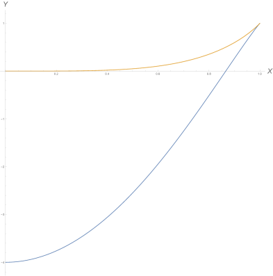
Figure 1: The rescaled energy density, $Y=\frac{27\Delta\phi^{3}}{8\pi^{3}\ell^{2}}\langle T_{tt}\rangle$, vs the rescaled magnetic flux, $X=\Phi/\Phi_{max}$, for the two branches of soliton solutions. The lower branch crosses the axis at $X_{S}=\Phi_{S}/\Phi_{max}=\sqrt{3}/2$.

As for the AdS soliton, the energy $\langle T_{tt}\rangle=-\frac{\mu}{2\ell^{2}}$ should be interpreted as a Casimir energy of the ground state. We see that turning on a Wilson line initially increases (reduces the magnitude of) the Casimir energy, presumably by deforming the spectrum of fields charged under this $U(1)_{R}$ symmetry. It is surprising that for $\Phi>\Phi_{S}$ the energy is zero, independent of the Wilson line $\Phi$. The cancellation between bosons and fermions is restored at the supersymmetric point, but it’s unexpected that this continues for higher values of the Wilson line. It would be interesting to investigate this directly from the field theory perspective.

The other mystery is the precise nature of the ground state at $\Phi=\Phi_{S}$. In our supergravity analysis, we have two degenerate solutions. This is the first example we know of with distinct supersymmetric solutions with the same boundary conditions, which are degenerate in energy. It is possible that this degeneracy is lifted by subleading effects, for example by considering the Casimir energy for bulk fields on these two geometries. This is certainly an interesting issue to investigate, but it seems unlikely that this will lift the degeneracy: the bulk solutions are supersymmetric, so the natural guess is that contributions to the bulk Casimir from bosonic and fermionic fields will cancel. Also, there is a phase transition between the two solutions which is at least very near the supersymmetric point; it would be surprising if it were then not precisely at this point. The alternative possibility is that the supersymmetric ground state in the field theory is dual to a superposition of these two geometries. This would be very interesting if true: the calculation of observables, such as correlation functions, in this ground state, would then involve contributions from both geometries. If these observables could be calculated on the CFT side, they would give a unique probe of relative phase information in the superposition of bulk geometries.

It is also interesting to note that the Poincaré-AdS solution is supersymmetric for $\Phi=2\pi n\ell$. Since $\Phi$ is periodic with period $8\pi\ell$, there are four physically inequivalent values giving supersymmetric solutions, which we can take to be $n=-1,0,1,2$. For odd $n$, the unbroken Killing spinors in Poincaré-AdS are antiperiodic on the $\phi$ circle, while for even $n$, they are periodic. For the odd cases, there is a degenerate soliton solution, but for the even cases Poincaré-AdS is the only supersymmetric solution. It would be interesting to understand this difference between odd and even $n$ from the field theory perspective.

2.5 Euclidean partition function

It is also interesting to consider the phase structure from a Euclidean perspective, to make contact with previous work on supersymmetric partition functions [13, 14, 16]. Previous work on this area has focused on the Euclidean theory with an $S^{1}\times\Sigma_{g}$ boundary, where $\Sigma_{g}$ is a Riemann surface of genus $g>1$, but this was extended to consider genus 1 in [10], corresponding to the case we have considered so far. We will comment on the extension of our discussion to higher genus in section 3.

The Euclidean continuation of our solutions are solutions with an $S^{1}\times\mathbb{R}^{2}$ boundary. These are usually treated thinking of the $S^{1}$ as the Euclidean time circle, so $\Phi$ is a chemical potential for the R-charge of the theory and the boundary path integral is interpreted as the partition function $Z=\mathrm{Tr}\,e^{i\Phi J_{R}}e^{-\Delta\phi\,H}$ of the CFT on $\mathbb{R}^{2}$. For $\Phi=2\pi\ell$, this partition function becomes a supersymmetric index.

In the saddle-point approximation, $Z\approx e^{-S_{E}}$, where $S_{E}$ is the action of the Euclidean solutions. For the solitons, the Wick rotated metric is

$$ds^{2}=\frac{r^{2}}{\ell^{2}}\left(d\tau^{2}+dz^{2}\right)+\frac{dr^{2}}{f(r)}+f(r)d\phi^{2}\,,$$ (42)

with $f(r)=\frac{r^{2}}{\ell^{2}}-\frac{Q^{2}}{r^{2}}-\frac{\mu}{r}$ as before. The Euclidean action is

$$\frac{S_{E}}{V} =-\lim_{R\rightarrow\infty}\left[\left(\int_{r_{0}}^{R}dr\sqrt{g_{E}}\frac{R}{2}-\frac{1}{8}F_{\mu\nu}F^{\mu\nu}+\frac{3}{\ell^{2}}\right)+\left(K\sqrt{h}-\frac{2}{\ell}\sqrt{h}\right)_{r=R}\right]$$

$$=-\frac{\mu}{2\ell^{2}},$$ (43)

where $V$ is the coordinate volume element on the boundary, $V=\int d\tau d\phi dz$. The Poincaré-AdS solution with a constant Wilson line always has zero action. Since the Euclidean action is proportional to $\mu$, the phase structure is the same as in our Lorentzian discussion above; for $\Phi\in[0,\Phi_{S})$, the dominant saddle-point is the lower soliton branch, for $\Phi\in(\Phi_{S},4\pi\ell]$ it is Poincaré-AdS. There is a phase transition at $\Phi=\Phi_{S}$.

For the supersymmetric case $\Phi=\Phi_{S}$, the partition function is an index, which can be computed by supersymmetric localization. For the present case, the CFT calculation gives an answer which vanishes to leading order in $N$ [12], in agreement with the bulk calculation. This calculation has previously been matched to the bulk result from Poincaré-AdS; we observe that both bulk saddles match the CFT result, and as discussed previously it will be interesting to understand further what the precise bulk dual of the index is.

An interesting issue here is the calculation of the expectation value of the $R$ charge in the ensemble. In the CFT, we can calculate the partition function exactly only at $\Phi=\Phi_{S}$, so we can’t extract a value for the R-charge from this; thermodynamically, to calculate the R-charge we need to consider the variation $\frac{\partial Z}{\partial\Phi}$. Holographically, we can evaluate the partition function for general $\Phi$, but at the supersymmetric point the degeneracy prevents us from evaluating the R-charge. The soliton saddle has $\langle J_{\phi}\rangle=2Q$, corresponding to a non-zero R-charge density, while Poincaré-AdS has $\langle J_{\phi}\rangle=0$. Since they are degenerate at $\Phi=\Phi_{S}$, we don’t know what value to use. Thermodynamically, the phase transition implies $Z$ is not a smooth function of $\Phi$, so $\frac{\partial Z}{\partial\Phi}$ is ill-defined at $\Phi=\Phi_{S}$.

2.6 Fixed charge

Since we are in four bulk dimensions, we can also define a holographic correspondence with alternative boundary conditions, where we fix $F^{\nu}\equiv\sqrt{h}n_{\mu}F^{\mu\nu}$ at the boundary (where $n_{\mu}$ is the unit normal to the boundary), instead of fixing $A_{\mu}$ [25]. This corresponds to fixing $\Delta\phi$ and $Q$. With these boundary conditions, Poincaré-AdS is not a solution. For the soliton solutions, we can solve (17) to determine $r_{0}$ as a function of $\Delta\phi$ and $Q$. We can see that $\Delta\phi$ is small at both $r_{0}\to 0$ and $r_{0}\to\infty$, with a maximum at $r_{0}^{4}=Q^{2}\ell^{2}$, which implies $\mu=0$, where $\Delta\phi=\Delta\phi_{max}=\pi\sqrt{\frac{\ell^{3}}{Q}}$. Thus, the supersymmetric solution in this case corresponds to the maximum value of $\Delta\phi$.

In the Euclidean action, we need to add a boundary term associated with the change in boundary conditions [25]

$$\frac{S_{\partial}}{V}=-\lim_{R\rightarrow\infty}\left(\frac{1}{2}\sqrt{h}N_{\mu}A_{\nu}F^{\mu\nu}\right)_{r=R}=-\frac{2Q^{2}}{\ell^{2}r_{0}},$$ (44)

so

$$S^{\prime}=S+S_{\partial}=-\left(\frac{\mu}{2\ell^{2}}+\frac{2Q^{2}}{\ell^{2}r_{0}}\right)V.$$ (45)

In figure 2, we plot the action for these solutions as a function of $\Delta\phi$ at fixed $Q$. We see that there are again two branches of solutions, coalescing at the supersymmetric solution at $\Delta\phi=\Delta\phi_{max}$. The lower branch corresponds to the solutions with $\mu<0$, which are always the dominant saddle for these boundary conditions.

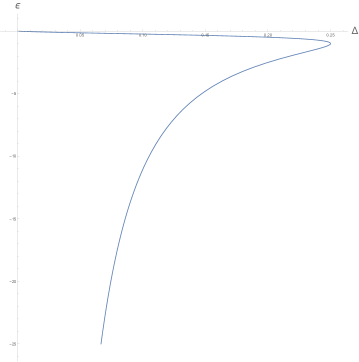
Figure 2: The action $\epsilon=\frac{\ell}{2\pi\left|Q\right|}S^{\prime}/V$ vs $\Delta=\frac{\sqrt{\left|Q\right|\ell}}{4\pi\ell^{2}}\Delta\phi$, at fixed $Q$. There are two solitons for each boundary condition for $\Delta\phi<\Delta\phi_{max}$. The supersymmetric solution is at the maximum value $\Delta\phi=\Delta\phi_{max}$.

3 Generalization to higher genus

It is straightforward to extend this discussion to the Euclidean partition function of the field theory on $S^{1}\times\Sigma_{g}$, where $\Sigma_{g}$ is a Riemann surface of genus $g>1$, studied in [13, 14, 12, 10]. The non-linear form of Euclidean gauged $\mathcal{N}=2$ supergravity was constructed in [26]. The relevant solutions are obtained from the analytic continuation of a black hole with horizon $\Sigma_{g}$, carrying both electric and magnetic charges,

$$ds^{2}=r^{2}ds^{2}_{\Sigma_{g}}+\frac{dr^{2}}{f(r)}+f(r)d\phi^{2},$$ (46)

with

$$f(r)=\frac{r^{2}}{\ell^{2}}-1-\frac{\mu}{r}+\frac{P^{2}-Q^{2}}{r^{2}},$$ (47)

where $ds^{2}_{\Sigma_{g}}$ is the unit constant negative curvature metric on $\Sigma_{g}$, and we have a gauge field

$$F=2P\epsilon_{\Sigma_{g}}+\frac{2Q}{r^{2}}d\phi\wedge dr,$$ (48)

where $\epsilon_{\Sigma_{g}}$ is the volume form of $ds^{2}_{\Sigma_{g}}$. Note that in the analytic continuation, we have analytically continued the electric charge $Q$ but not the magnetic charge $P$, hence the difference in sign in the metric function. We want to restrict the parameters so that $f(r)$ has at least one real positive root; we take as before $r_{0}$ to be the largest positive root, $f(r_{0})=0$.

The solution considered in [12] has $\mu=Q=0$, and $P=\pm\ell/2$. This is a supersymmetric black hole, first studied in [7]; the contributions of the field strength and the spin connection on $\Sigma_{g}$ in (8) cancel, to allow us to find two chiral Killing spinors, namely the solution is $1/4$ BPS. For these parameters, $f(r)$ has a double root at $r_{0}=\ell/\sqrt{2}$,

$$f(r)=\left(\frac{r}{\ell}-\frac{\ell}{2r}\right)^{2}.$$ (49)

The geometry near $r=r_{0}$ is thus $H^{2}\times\Sigma_{g}$; in Lorentzian signature, this is an extremal black hole, with a near-horizon $AdS_{2}$ region.

The solution is regular for $\phi\in\mathbb{R}$, but we can obtain solutions with periodic $\phi$ by quotienting this solution, as in our previous discussion of Poincaré-AdS. As before, we can consider adding a Wilson line along the $\phi$ circle in the quotient; this corresponds to a chemical potential for the R-charge in the partition function. This quotient will have unbroken supersymmetry if $\Phi=2\pi n\ell$ for integer $n$. Recall that $\Phi$ is periodic with period $8\pi\ell$, so there are four physically inequivalent values giving supersymmetric solutions, which we can take to be $n=-1,0,1,2$. For odd $n$, the unbroken Killing spinors are antiperiodic on the $\phi$ circle, while for even $n$, they are periodic.

In [10], the solutions with $\mu=0$ but non-zero $Q$ were considered;

$$f(r)=\left(\frac{r}{\ell}-\frac{\ell}{2r}\right)^{2}-\frac{Q^{2}}{r^{2}}$$ (50)

with

$$A=A_{\Sigma_{g}}+\left(\frac{2Q}{r}-\frac{2Q}{r_{0}}\right)d\phi,$$ (51)

where $A_{\Sigma_{g}}$ is a gauge potential on the Riemann surface giving the magnetic part of $F$. The largest root of $f$ is at

$$r_{0}=\frac{\ell}{\sqrt{2}}\sqrt{1+|Q|/\sqrt{2}\ell}.$$ (52)

This is now a single root, so the geometry near $r=r_{0}$ is $\mathbb{R}^{2}\times\Sigma_{g}$, and we need to choose $\phi$ periodic with period

$$\Delta\phi=\frac{4\pi}{f^{\prime}(r_{0})}=\frac{\pi\ell r_{0}}{|Q|}.$$ (53)

There is a boundary Wilson line $\Phi=\frac{2Q}{r_{0}}\Delta\phi=\pm 2\pi\ell$, and the solution is supersymmetric, with antiperiodic Killing spinors.

Thus, as in the earlier discussion, there are two supersymmetric solutions with antiperiodic Killing spinors for $\Phi=\pm 2\pi\ell$; the quotiented solution with $Q=0$ and the soliton-like solution with non-zero $Q$. The action of these solutions is equal [10],

$$S_{E}=-\frac{\sqrt{2}\pi}{3}(g-1)N^{3/2}.$$ (54)

This reproduces the value of the twisted topological index calculated in the field theory using localization methods [14]. It is in principle straightforward to extend this analysis to more general solutions with scalars, although explicitly constructing the soliton solutions is challenging [10].

As in the genus one case, it would be very interesting to understand further the degeneracy between these two solutions. It would also be interesting to understand the difference between odd $n$ (where we have this degeneracy) and even $n$ (where the $Q=0$ solution is the unique supersymmetric solution) from the field theory perspective.

If we want to consider different values of $\Phi$, we can detune this solution by considering the geometry with $\mu$ also non-zero,

$$f(r)=\left(\frac{r}{\ell}-\frac{\ell}{2r}\right)^{2}-\frac{\mu}{r}-\frac{Q^{2}}{r^{2}}.$$ (55)

We leave a complete understanding of the space of possible smooth non-supersymmetric solutions for future work; it is not trivial in this case to solve for $\mu,Q$ in terms of the natural boundary parameters $\Delta\phi,\Phi$, or to establish the range of parameters for which there is a positive root $r_{0}$.

4 Five dimensions

4.1 Minimal gauged supergravity

The discussion so far has been in four bulk dimensions; it is easy to generalise the construction to higher dimensions. Here we will consider in particular Einstein-Maxwell-AdS in five bulk dimensions constructed in several papers [27, 28, 29, 30, 31, 32, 33, 34]. We follow [9, 22]. The action principle is

$$S\left(g,A\right)=\frac{1}{8\pi G}\int d^{5}x\left(\sqrt{-g}\left[\frac{R}{2}+\frac{6}{\ell^{2}}-\frac{1}{8}F_{\mu\nu}F^{\mu\nu}\right]+\frac{1}{24\sqrt{3}}F\wedge F\wedge A\right)\text{ },$$ (56)

with field equations

$$\partial_{\mu}\big{(}\sqrt{-g}F^{\mu\nu}\big{)}=0\,\,,$$

$$R_{\mu\nu}-\tfrac{1}{2}g_{\mu\nu}R-\tfrac{1}{2}\big{[}F_{\mu\rho}\,F_{\nu}{}^{\rho}-\tfrac{1}{4}g_{\mu\nu}F_{\rho\sigma}F^{\rho\sigma}\big{]}-\frac{6}{\ell^{2}}\,g_{\mu\nu}=0\,.$$ (57)

where we have used that our solutions shall satisfy $F\wedge F=0$. In our conventions, the Killing spinor equations can be written in terms of a single complex spinor, $\Psi$, as follows

$$\big{(}\partial_{\mu}+\tfrac{1}{4}\omega_{\mu}{\!}^{ab}\gamma_{ab}-\frac{\mathrm{i}}{8\sqrt{3}}\gamma_{\mu\lambda\alpha}F^{\lambda\alpha}+\frac{\mathrm{i}}{2\sqrt{3}}F_{\mu\alpha}\gamma^{\alpha}\big{)}\Psi+\ell^{-1}\left(\frac{\mathrm{i}}{2}\gamma_{\mu}-\frac{\sqrt{3}}{2}A_{\mu}\,\right)\gamma^{4}\Psi^{\ast}=0\text{ .}$$ (58)

where $\gamma^{4}=\mathrm{i}\gamma^{0}\gamma^{1}\gamma^{2}\gamma^{3}$ is the gamma matrix along the fifth dimension and $\Psi^{\ast}$ is the complex conjugate of $\Psi$.

The theory we considered here is obtained by a dimensional reduction of type IIB supergravity over the five-sphere with the ansatz [22]

$$ds_{10}^{2} =ds_{5}^{2}+\ell^{2}\sum_{i=1}^{3}d\mu_{i}^{2}+\mu_{i}^{2}(d\phi_{i}+\frac{1}{\sqrt{3}\ell}A)^{2}$$ (59)

$$F_{5} =G_{5}+\ast_{5}G_{5}$$ (60)

$$G_{5} =-\frac{4}{\ell}\epsilon_{5}+\frac{\ell^{2}}{\sqrt{3}}\sum_{i=1}^{3}\mu_{i}d\mu_{i}\wedge(d\phi_{i}+\frac{1}{\sqrt{3}\ell}A)\wedge\ast_{5}dA$$ (61)

where  $\ast_{5}$ is the Hodge dual with respect to the five-dimensional metric $ds_{5}^{2}$ and $\epsilon_{5}$ is its volume form.

4.2 Soliton solutions

By double analytic continuation of the electrically charged black hole solutions with a flat boundary, we obtain a solution

$$ds^{2}=\frac{r^{2}}{\ell^{2}}(-dt^{2}+dy^{2}+dz^{2})+\frac{dr^{2}}{f(r)}+f(r)d\phi^{2},$$ (62)

where

$$f(r)=\frac{r^{2}}{\ell^{2}}-\frac{\mu}{r^{2}}-\frac{q^{2}}{r^{4}}.$$ (63)

This is a solution of Einstein-Maxwell with the gauge field

$$A=\left(\frac{\sqrt{3}q}{r^{2}}-\frac{\sqrt{3}q}{r_{0}^{2}}\right)d\phi,$$ (64)

where $r_{0}$ is the largest root of $f(r)$, $f(r_{0})=0$. We can write

$$\mu=\frac{(r_{0}^{6}-q^{2}\ell^{2})}{\ell^{2}r_{0}^{2}}.$$ (65)

The solution is smooth at $r=r_{0}$ if $\phi$ has period

$$\Delta\phi=\frac{4\pi}{f^{\prime}(r_{0})}.$$ (66)

The flux through the $\phi$ circle at $r\rightarrow\infty$ is $\Phi=\oint A=\frac{\sqrt{3}q}{r_{0}^{2}}\Delta\phi$. The boundary data is $\Delta\phi$ and $\Phi$, so it is convenient to re-express the bulk parameters in terms of these; we have

$$q=\frac{r_{0}^{2}}{\sqrt{3}}\frac{\Phi}{\Delta\phi},$$ (67)

with

$$r_{0}=\frac{\pi\ell^{2}}{2\Delta\phi}\left(1\pm\sqrt{1-\frac{\Phi^{2}}{\Phi_{max}^{2}}}\right),$$ (68)

where $\Phi_{max}=\sqrt{\frac{3}{2}}\pi\ell$. We see that for $\Phi<\Phi_{max}$, there are two branches of solutions. The $+$ branch approaches the AdS soliton as $\Phi\rightarrow 0$, while the $-$ branch approaches Poincaré - AdS, and they coalesce at $\Phi=\Phi_{max}$. We have $\mu=0$ when $r_{0}^{6}=q^{2}\ell^{2}$, that is when

$$r_{0}^{2}=\frac{\Phi^{2}\ell^{2}}{3\Delta\phi^{2}}\quad\Rightarrow\quad 2-3\frac{\Phi^{2}}{\Phi_{max}^{2}}\pm 2\sqrt{1-\frac{\Phi^{2}}{\Phi_{max}^{2}}}=0,$$ (69)

which is satisfied on the $+$ branch at $\Phi=\Phi_{S}=\frac{2\sqrt{2}}{3}\Phi_{max}$, that is $\Phi_{S}=\frac{2\pi}{\sqrt{3}}\ell$.

4.3 Supersymmetric solutions

To solve the Killing spinor equation at the supersymmetric point $\mu=0$, we introduce the change of coordinates

$$r=\left|q\ell\right|^{2/3}\cosh(\rho)^{1/3},$$ (70)

in terms of which the metric and gauge field read

$$ds^{2} =\frac{\ell^{2}}{9}d\rho^{2}+\frac{r_{0}^{2}}{\ell^{2}}\left[\cosh\left(\rho\right)^{2/3}\left(-dt^{2}+dy^{2}+dz^{2}\right)+\frac{\sinh\left(\rho\right)^{2}}{\cosh(\rho)^{4/3}}d\phi^{2}\right],$$ (71)

$$A =\frac{\sqrt{3}q}{r_{0}^{2}}\left(\frac{1}{\cosh(\rho)^{2/3}}-1\right)d\phi,$$ (72)

where in this section we take $r_{0}=\left|q\ell\right|^{1/3}$ and $\Delta\phi=\frac{2\pi\ell^{5/3}}{3q^{1/3}}$. The calculation shall be carried in the same basis as in the $D=4$ with the extra vielbein

$$e^{4}=\frac{r_{0}}{\ell}\cosh(\rho)^{1/3}dy\text{ .}$$ (73)

There are four independent solutions to the Killing spinor equation on this background:

$$\Psi_{1} =\cosh(\rho)^{-1/3}\left(\begin{array}[c]{c}s_{\rho}c_{\phi}+\mathrm{i}c_{\rho}s_{\phi}\\ -c_{\rho}c_{\phi}+\mathrm{i}s_{\rho}s_{\phi}\\ c_{\rho}s_{\phi}-\mathrm{i}s_{\rho}c_{\phi}\\ s_{\rho}s_{\phi}+\mathrm{i}c_{\rho}c_{\phi}\end{array}\right)\text{ },\qquad\Psi_{2}=\cosh(\rho)^{-1/3}\left(\begin{array}[c]{c}c_{\rho}c_{\phi}+\mathrm{i}s_{\rho}s_{\phi}\\ -s_{\rho}c_{\phi}+\mathrm{i}c_{\rho}s_{\phi}\\ -s_{\rho}s_{\phi}+\mathrm{i}c_{\rho}c_{\phi}\\ -c_{\rho}s_{\phi}-\mathrm{i}s_{\rho}c_{\phi}\end{array}\right),$$ (82)

$$\Psi_{3} =\cosh(\rho)^{-1/3}\left(\begin{array}[c]{c}s_{\rho}s_{\phi}-\mathrm{i}c_{\rho}c_{\phi}\\ -c_{\rho}s_{\phi}-\mathrm{i}s_{\rho}c_{\phi}\\ -c_{\rho}c_{\phi}-\mathrm{i}s_{\rho}s_{\phi}\\ -s_{\rho}c_{\phi}+\mathrm{i}c_{\rho}s_{\phi}\end{array}\right)\text{ },\qquad\Psi_{4}=\cosh(\rho)^{-1/3}\left(\begin{array}[c]{c}c_{\rho}s_{\phi}-\mathrm{i}s_{\rho}c_{\phi}\\ -s_{\rho}s_{\phi}-\mathrm{i}c_{\rho}c_{\phi}\\ s_{\rho}c_{\phi}+\mathrm{i}c_{\rho}s_{\phi}\\ c_{\rho}c_{\phi}-\mathrm{i}s_{\rho}s_{\phi}\end{array}\right)\text{ ,}$$ (91)

where $s_{\rho}=\sinh\left(\frac{\rho}{2}\right)$, $c_{\rho}=\cosh\left(\frac{\rho}{2}\right)$, $s_{\phi}=\sin\left(\frac{\pi}{\Delta\phi}\phi\right)$ and $c_{\phi}=\cos\left(\frac{\pi}{\Delta\phi}\phi\right)$, which implies that the solution is $1/2$ BPS. As a cross-check we verify the formulae which relate Killing spinors and Killing vectors as given in section 2 of [9]. The most general Killing spinor for this solution is

$$\vskip 12.0pt plus 4.0pt minus 4.0pt\Psi=\sum_{i=1}^{4}c_{i}\Psi_{i}\text{ .}$$ (92)

where the $c_{i}$ are real constants. It statisfies that

$$\Psi^{T}\left(\gamma^{4}\right)^{\dagger}\gamma^{0}\Psi =0\text{ ,}$$ (93)

$$\Psi^{T}\left(\gamma^{4}\right)^{\dagger}\gamma^{0}\gamma^{\mu}\gamma^{4}\Psi^{\ast} =K^{\mu}\text{ ,}$$ (94)

where the components of the Killing vector are

$$K^{t} =\frac{2\ell}{r_{0}}\left(c_{1}^{2}+c_{2}^{2}+c_{3}^{2}+c_{4}^{2}\right)\text{ ,}$$ (95)

$$K^{\phi} =\frac{4\ell}{r_{0}}\left(c_{3}c_{4}+c_{1}c_{2}\right)\text{ ,}$$ (96)

$$K^{z} =-\frac{4\ell}{r_{0}}\left(c_{1}c_{4}-c_{3}c_{2}\right)\text{ ,}$$ (97)

$$K^{y} =-\frac{2\ell}{r_{0}}\left(c_{1}^{2}-c_{2}^{2}+c_{3}^{2}-c_{4}^{2}\right)\text{ .}$$ (98)

Let us note that in an asymptotic expansion, the leading term of the spinors is

$$\lim_{\rho\rightarrow\infty}e^{-\frac{\rho}{6}}\Psi_{1} =\left(\begin{array}[c]{c}\exp\left(\mathrm{i}\frac{\pi}{\Delta\phi}\phi\right)\\ -\exp\left(-\mathrm{i}\frac{\pi}{\Delta\phi}\phi\right)\\ -\mathrm{i}\exp\left(\mathrm{i}\frac{\pi}{\Delta\phi}\phi\right)\\ \mathrm{i}\exp\left(-\mathrm{i}\frac{\pi}{\Delta\phi}\phi\right)\end{array}\right),\qquad\lim_{\rho\rightarrow\infty}e^{-\frac{\rho}{6}}\Psi_{2}=\left(\begin{array}[c]{c}\exp\left(\mathrm{i}\frac{\pi}{\Delta\phi}\phi\right)\\ -\exp\left(-\mathrm{i}\frac{\pi}{\Delta\phi}\phi\right)\\ \mathrm{i}\exp\left(\mathrm{i}\frac{\pi}{\Delta\phi}\phi\right)\\ -\mathrm{i}\exp\left(-\mathrm{i}\frac{\pi}{\Delta\phi}\phi\right)\end{array}\right),$$ (107)

$$\lim_{\rho\rightarrow\infty}e^{-\frac{\rho}{6}}\Psi_{3} =\left(\begin{array}[c]{c}-\mathrm{i}\exp\left(\mathrm{i}\frac{\pi}{\Delta\phi}\phi\right)\\ -\mathrm{i}\exp\left(-\mathrm{i}\frac{\pi}{\Delta\phi}\phi\right)\\ -\exp\left(\mathrm{i}\frac{\pi}{\Delta\phi}\phi\right)\\ -\exp\left(-\mathrm{i}\frac{\pi}{\Delta\phi}\phi\right)\end{array}\right),\qquad\lim_{\rho\rightarrow\infty}e^{-\frac{\rho}{6}}\Psi_{4}=\left(\begin{array}[c]{c}-\mathrm{i}\exp\left(\mathrm{i}\frac{\pi}{\Delta\phi}\phi\right)\\ -\mathrm{i}\exp\left(-\mathrm{i}\frac{\pi}{\Delta\phi}\phi\right)\\ \exp\left(\mathrm{i}\frac{\pi}{\Delta\phi}\phi\right)\\ \exp\left(-\mathrm{i}\frac{\pi}{\Delta\phi}\phi\right)\end{array}\right)\text{.}$$ (116)

On pure AdS₅, the theory has four Killing spinors; if we introduce a Wilson loop on this background with $A=A_{\phi}d\phi$. Indeed, a basis for the local solutions to the Killing spinor equation in the Poincaré patch are

$$\Psi_{1+}^{AdS}=\Delta_{+}\left(\begin{array}[c]{c}0\\ 1\\ 0\\ 0\end{array}\right),\text{ }\Psi_{1-}^{AdS}=\Delta_{-}\left(\begin{array}[c]{c}-1\\ 0\\ 0\\ 0\end{array}\right),\text{ }\Psi_{2+}^{AdS}=\Delta_{+}\left(\begin{array}[c]{c}0\\ 0\\ 0\\ 1\end{array}\right),\text{ }\Psi_{2-}^{AdS}=\Delta_{-}\left(\begin{array}[c]{c}0\\ 0\\ 1\\ 0\end{array}\right)\text{,}$$ (117)

$$\Psi_{3+}^{AdS} =\Delta_{+}\left(\begin{array}[c]{c}0\\ \phi+t\\ \ell^{2}r^{-1}\\ z+\mathrm{i}y\end{array}\right),\text{ }\Psi_{3-}^{AdS}=\Delta_{-}\left(\begin{array}[c]{c}-\phi-t\\ 0\\ z-\mathrm{i}y\\ -\ell^{2}r^{-1}\end{array}\right),$$ (126)

$$\Psi_{4+}^{AdS} =\Delta_{+}\left(\begin{array}[c]{c}\ell^{2}r^{-1}\\ z-\mathrm{i}y\\ 0\\ t-\phi\end{array}\right),\Psi_{4-}^{AdS}=\Delta_{-}\left(\begin{array}[c]{c}-z-\mathrm{i}y\\ \ell^{2}r^{-1}\\ -\phi+t\\ 0\end{array}\right)\text{ }.$$ (135)

where $\Delta_{\pm}=\sqrt{r}\exp\left(\pm\mathrm{i}\frac{\sqrt{3}A_{\phi}}{2\ell}\phi\right)$. The most general solution to the Killing spinor equation in this basis is

$$\Psi^{AdS}=\sum_{i=1}^{4}\alpha_{i}\Psi_{i+}^{AdS}+\sum_{i=1}^{4}\alpha_{i}^{\ast}\Psi_{i-}^{AdS}$$ (136)

where the constants $\alpha_{i}^{\ast}$ are the complex conjugate of $\alpha_{i}$. Again we can see from the Killing spinors that the identification in $\phi$ breaks half of the supersymmetries of AdS₅.

For $\Phi=\Phi_{S}=\frac{2\pi}{\sqrt{3}}\ell$, we can also obtain a supersymmetric solution from Poincaré-AdS with a constant Wilson loop along the $\phi$ circle in the bulk. As in four dimensions, this is easily seen from the uplift of the theory to ten dimensions. The theory we considered here is obtained by a dimensional reduction [22]

$$ds_{10}^{2}=ds_{5}^{2}+\ell^{2}\sum_{i=1}^{3}d\mu_{i}^{2}+\mu_{i}^{2}(d\phi_{i}+\frac{1}{\sqrt{3}\ell}A)^{2};$$ (137)

The coordinates $\phi_{i}$ are $2\pi$ periodic. The ten-dimensional metric is thus invariant under shifts of the Wilson loop by $\Phi\rightarrow\Phi+2\pi\sqrt{3}\ell$, making this a periodic variable. Quotienting Poincaré-AdS with a Wilson loop on the $\phi$ circle corresponds to a quotient of $AdS_{5}\times S^{5}$ by $(\phi,\tilde{\phi}_{i})\sim(\phi+\Delta\phi,\tilde{\phi}_{i}+\Phi/\sqrt{3}\ell)$, so the ten-dimensional Killing spinors will be invariant under the quotient if $\Phi=\frac{2\pi}{\sqrt{3}}n\ell$ for integer $n$. Given the periodicity of $\Phi$, there are three physically inequivalent cases, $n=-1,0,1$. For $n=-1,1$, we have a degeneracy between the Poincaré-AdS solution and the supersymmetric soliton. The main qualitative difference between the four- and five-dimensional cases is that we only have one case with a unique supersymmetric solution here.

5 Conclusions

We have shown that the simplest $D=4$ and $D=5$ gauged supergravities theories, which allow for charged solutions, contain in its spectrum of supersymmetric solutions Lorentzian planar solitons. These solitons can be seen as a supersymmetric extension of the rather well-known AdS soliton of Horowitz and Myers [2]. The existence of these supersymmetric solitons poses an holographic puzzle. One usually expects that for given boundary conditions, at least with sufficient supersymmetry, the gravitational solution would be completely fixed. This solution would then be dual to a supersymmetric state in the dual CFT. However, as we have explictly shown this is not the case. One possible way out would be if the solutions were supersymmetric with respect to different realizations of the supersymmetry algebra in $AdS_{4}$ [35]. However in the different realizations, for the same supersymmetry and same boundary conditions for the metric, the form of the Killing spinors is different. Our explicit construction of the Killing spinors shows that the soliton Killing spinors are asymptotically the Killing spinors of a locally AdS spacetime. Hence, these configurations are indeed completely indistiguishable from the boundary point of view. Moreovoer, the Killing spinors for the solitons provide an smooth interpolation between some Killing spinors of Minkowski_D and AdS_D, for $D=4$ and $D=5$.

The simplicity of the susy AdS soliton make us conjecture that these $1/2$ BPS solutions can be generalized to have different charges by the introduction of running scalars in $D=4$ and $D=5$ gauged supergravity [22, 36, 37, 38]. Furthermore, we believe that this susy AdS soliton should also be part of the spectrum of any gauged supergravity in any dimension that contains a consistent supersymmetric truncation with a $U(1)$ gauge field. Therefore the degeneracy of susy states we presented here, it is very likely, a generic feature of these boundary conditions.

The structure of the soliton seems to be well suited to be interpreted in the context of holographic superconductivity [39]. Indeed, from the holographic point of view, the boundary of the soliton is a cylinider with a current flowing along the circle. The current is flowing without any electromagnetic field on the surface of the cylinder and there is a magnetic field piercing the cylinder. It would be worth understanding if the periodic oscillation of the critical temperature of the superconductor takes place holographically as expected due to the Little-Parks effect [40].

An interesting question to be further explored is whether other boundary conditions can yield a degeneration in the spectrum of supersymmetric solutions. Asymptotically locally AdS, everywhere regular supersymmetric solutions in the pure Einstein-Maxwell theory with a negative cosmological constant exist in four dimensions but with a much more complex structure than the one discussed here [41].

References

- [1] E. Witten, “Instability of the Kaluza-Klein Vacuum,” Nucl. Phys. B 195 (1982) 481–492.
- [2] G. T. Horowitz and R. C. Myers, “The AdS / CFT correspondence and a new positive energy conjecture for general relativity,” Phys. Rev. D 59 (1998) 026005, arXiv:hep-th/9808079.
- [3] M. A. Melvin, “Pure magnetic and electric geons,” Phys. Lett. 8 (1964) 65–70.
- [4] M. Astorino, “Charging axisymmetric space-times with cosmological constant,” JHEP 06 (2012) 086, arXiv:1205.6998 [gr-qc].
- [5] Y.-K. Lim, “Electric or magnetic universe with a cosmological constant,” Phys. Rev. D 98 no. 8, (2018) 084022, arXiv:1807.07199 [gr-qc].
- [6] D. Kastor and J. Traschen, “Geometry of AdS-Melvin Spacetimes,” Class. Quant. Grav. 38 no. 4, (2021) 045016, arXiv:2009.14771 [hep-th].
- [7] L. J. Romans, “Supersymmetric, cold and lukewarm black holes in cosmological Einstein-Maxwell theory,” Nucl. Phys. B 383 (1992) 395–415, arXiv:hep-th/9203018.
- [8] M. M. Caldarelli and D. Klemm, “Supersymmetry of Anti-de Sitter black holes,” Nucl. Phys. B 545 (1999) 434–460, arXiv:hep-th/9808097.
- [9] J. P. Gauntlett and J. B. Gutowski, “All supersymmetric solutions of minimal gauged supergravity in five-dimensions,” Phys. Rev. D 68 (2003) 105009, arXiv:hep-th/0304064. [Erratum: Phys.Rev.D 70, 089901 (2004)].
- [10] N. Bobev, A. M. Charles, and V. S. Min, “Euclidean black saddles and AdS4 black holes,” JHEP 10 (2020) 073, arXiv:2006.01148 [hep-th].
- [11] S. L. Cacciatori and D. Klemm, “Supersymmetric AdS(4) black holes and attractors,” JHEP 01 (2010) 085, arXiv:0911.4926 [hep-th].
- [12] F. Benini, K. Hristov, and A. Zaffaroni, “Black hole microstates in AdS4 from supersymmetric localization,” JHEP 05 (2016) 054, arXiv:1511.04085 [hep-th].
- [13] F. Benini and A. Zaffaroni, “A topologically twisted index for three-dimensional supersymmetric theories,” JHEP 07 (2015) 127, arXiv:1504.03698 [hep-th].
- [14] F. Benini and A. Zaffaroni, “Supersymmetric partition functions on Riemann surfaces,” Proc. Symp. Pure Math. 96 (2017) 13–46, arXiv:1605.06120 [hep-th].
- [15] C. Closset and H. Kim, “Comments on twisted indices in 3d supersymmetric gauge theories,” JHEP 08 (2016) 059, arXiv:1605.06531 [hep-th].
- [16] A. Zaffaroni, “AdS black holes, holography and localization,” Living Rev. Rel. 23 no. 1, (2020) 2, arXiv:1902.07176 [hep-th].
- [17] D. Z. Freedman and A. K. Das, “Gauge Internal Symmetry in Extended Supergravity,” Nucl. Phys. B 120 (1977) 221–230.
- [18] E. S. Fradkin and M. A. Vasiliev, “Model of Supergravity with Minimal Electromagnetic Interaction,”.
- [19] B. de Wit, J. W. van Holten, and A. Van Proeyen, “Structure of N=2 Supergravity,” Nucl. Phys. B 184 (1981) 77. [Erratum: Nucl.Phys.B 222, 516 (1983)].
- [20] B. de Wit and A. Van Proeyen, “Potentials and Symmetries of General Gauged N=2 Supergravity: Yang-Mills Models,” Nucl. Phys. B 245 (1984) 89–117.
- [21] B. de Wit, P. G. Lauwers, and A. Van Proeyen, “Lagrangians of N=2 Supergravity - Matter Systems,” Nucl. Phys. B 255 (1985) 569–608.
- [22] M. Cvetic, M. J. Duff, P. Hoxha, J. T. Liu, H. Lu, J. X. Lu, R. Martinez-Acosta, C. N. Pope, H. Sati, and T. A. Tran, “Embedding AdS black holes in ten-dimensions and eleven-dimensions,” Nucl. Phys. B 558 (1999) 96–126, arXiv:hep-th/9903214.
- [23] A. Adams, J. Polchinski, and E. Silverstein, “Don’t panic! Closed string tachyons in ALE space-times,” JHEP 10 (2001) 029, arXiv:hep-th/0108075.
- [24] G. T. Horowitz and E. Silverstein, “The Inside story: Quasilocal tachyons and black holes,” Phys. Rev. D 73 (2006) 064016, arXiv:hep-th/0601032.
- [25] D. Marolf and S. F. Ross, “Boundary Conditions and New Dualities: Vector Fields in AdS/CFT,” JHEP 11 (2006) 085, arXiv:hep-th/0606113.
- [26] B. de Wit and V. Reys, “Euclidean supergravity,” JHEP 12 (2017) 011, arXiv:1706.04973 [hep-th].
- [27] J. H. Schwarz, “Covariant Field Equations of Chiral N=2 D=10 Supergravity,” Nucl. Phys. B 226 (1983) 269.
- [28] P. S. Howe and P. C. West, “The Complete N=2, D=10 Supergravity,” Nucl. Phys. B 238 (1984) 181–220.
- [29] J. H. Schwarz, “SPONTANEOUS COMPACTIFICATION OF EXTENDED SUPERGRAVITY IN TEN-DIMENSIONS,” in 12th International Congress on Mathematical Physics (IAMP). 8, 1983.
- [30] M. Gunaydin and N. Marcus, “The Spectrum of the s**5 Compactification of the Chiral N=2, D=10 Supergravity and the Unitary Supermultiplets of U(2, 2/4),” Class. Quant. Grav. 2 (1985) L11.
- [31] H. J. Kim, L. J. Romans, and P. van Nieuwenhuizen, “The Mass Spectrum of Chiral N=2 D=10 Supergravity on S**5,” Phys. Rev. D 32 (1985) 389.
- [32] M. Pernici, K. Pilch, and P. van Nieuwenhuizen, “Gauged N=8 D=5 Supergravity,” Nucl. Phys. B 259 (1985) 460.
- [33] M. Gunaydin, L. J. Romans, and N. P. Warner, “Gauged N=8 Supergravity in Five-Dimensions,” Phys. Lett. B 154 (1985) 268–274.
- [34] A. Baguet, O. Hohm, and H. Samtleben, “Consistent Type IIB Reductions to Maximal 5D Supergravity,” Phys. Rev. D 92 no. 6, (2015) 065004, arXiv:1506.01385 [hep-th].
- [35] K. Hristov, C. Toldo, and S. Vandoren, “On BPS bounds in D=4 N=2 gauged supergravity,” JHEP 12 (2011) 014, arXiv:1110.2688 [hep-th].
- [36] A. Anabalon, D. Astefanesei, D. Choque, and J. D. Edelstein, “Phase transitions of neutral planar hairy AdS black holes,” JHEP 07 (2020) 129, arXiv:1912.03318 [hep-th].
- [37] A. Anabalón, D. Astefanesei, D. Choque, A. Gallerati, and M. Trigiante, “Exact holographic RG flows in extended SUGRA,” JHEP 04 (2021) 053, arXiv:2012.01289 [hep-th].
- [38] A. Anabalon, D. Astefanesei, A. Gallerati, and M. Trigiante, “New non-extremal and BPS hairy black holes in gauged and supergravity,” JHEP 04 (2021) 047, arXiv:2012.09877 [hep-th].
- [39] S. A. Hartnoll, C. P. Herzog, and G. T. Horowitz, “Building a Holographic Superconductor,” Phys. Rev. Lett. 101 (2008) 031601, arXiv:0803.3295 [hep-th].
- [40] W. Little and R. Parks, “Observation of Quantum Periodicity in the Transition Temperature of a Superconducting Cylinder,” Physical Review Letters 9 (1962) 9.
- [41] A. Anabalón, B. de Wit, and J. Oliva, “Supersymmetric traversable wormholes,” JHEP 09 (2020) 109, arXiv:2001.00606 [hep-th].