One-loop corrections to light neutrino masses in gauged U(1) extensions of the standard model

Abstract

We consider gauged U(1) extensions of the standard model of particle physics with three right-handed sterile neutrinos and a singlet scalar. The neutrinos obtain mass via the type I seesaw mechanism. We compute the one loop corrections to the elements of the tree level mass matrix of the light neutrinos and show explicitly the cancellation of the gauge dependent terms. We present a general formula for the gauge independent, finite one-loop corrections for arbitrary number new U(1) groups, new complex scalars and sterile neutrinos. We estimate the size of the corrections relative to the tree level mass matrix in a particular extension, the super-weak model.

I Introduction

The standard model (SM) of particle interactions is one of the most successful physics models with unprecedented precision for predicting physical quantities, for instance for the anomalous magnetic moment of the electron. However, it does not contain right handed neutrinos as they are sterile under the SM gauge group. This in turn leads to the prediction that neutrinos are massless which is in conflict of the now well established experimental result, that at least two neutrinos are massive [1, 2], and therefore, signals that the SM requires an extension to explain the origin of the neutrino masses. There are lots of models attempting to explain neutrino masses. Among those perhaps the most economical one that requires the least extension of the SM, is the type I seesaw mechanism where neutrinos acquire masses after spontaneous symmetry breaking (SSB) of one or more scalar fields [3, 4, 5, 6, 7, 8, 9, 10].

Recently there has been a lot of interest in gauged U(1)-extended models in particle physics phenomenology, motivated by the observed difference between the measured and SM predicted values of the anomalous magnetic moment of the muon [11] and also anomalies in short-baseline neutrino oscillations [12]. Gauged $B-L$, $B-3L_{\tau}$, $L_{e}-L_{\mu}$ and $L_{\mu}-L_{\tau}$ have been considered [13, 14, 15, 16, 17, 18, 19], as well as a general gauged U(1) not related to flavour [20]. In these models, both seesaw and radiative one-loop neutrino mass generation mechanisms have been considered.

As the effects of new physics are typically much smaller than those of the SM interactions, computations in theories beyond the SM are often considered only at tree level. Yet, the loop corrections may be sizable and can affect significantly the validity region in the parameter space of the model. For instance, the lightness of active neutrinos requires that the loop corrections to the mass matrix of those particles must also be small in order to have a phenomenologically viable model. Computations of such one-loop corrections have been carried out previously in Refs. [21, 22] for the canonical seesaw case, and in the context of multi-Higgs doublet models [23, 24, 25, 26]. In the cases of gauged U(1) models we are not aware of a computation of the one-loop corrections to active neutrino mass matrix.

In this article we consider gauged U(1) extensions of the SM and derive a general formula for the one-loop corrections of the mass matrix of the active neutrinos. The mass matrix of the active neutrinos emerges after SSB due to the type I seesaw mechanism. Our goal is to derive the one-loop corrections to that mass matrix and estimate their sizes relative to the tree level for a particular example, called the super-weak force [27]. The super-weak model contains three additional right-handed sterile (under the SM interactions) neutrinos and one complex scalar field in addition to the fields of the SM. The loop corrections involve all the gauge and scalar bosons which couple to neutrinos.

In order to obtain the one-loop corrections to the elements of the light neutrino mass matrix, we perform our computations in the $R_{\xi}$ gauge and show explicitly the intricate cancellation of the gauge fixing parameters from the corrections. In addition, we shall also demonstrate the cancellation of the $\epsilon$ poles when the loop integrals are regulated by dimensional regularization in $d=4-2\epsilon$ dimensions. These cancellations are highly non-trivial, and therefore provide strong checks on the correctness of the computations.

The paper is composed as follows. We introduce the model to the extent needed for the present work in Sect. II. We define and compute the one loop correction to mass matrix of the active neutrinos in Sect. III. In Sect. IV we provide numerical estimates of the one-loop corrections and show that those are very small. Finally we summarize our findings in Sec. V. We collect auxiliary formulas in the appendices and also provide an auxiliary zip file containing the SARAH model, parameter and particle files.

II Particle model, mixings and interactions

We consider an extension of the standard model by a U(1)_z gauge group with particle content and charge assignment defined in Ref. [27]. The super-weak model is an economical extension of the standard model that provides a framework to explain the origin of (i) neutrino masses and oscillations [28], (ii) dark matter [29], (iii) cosmic inflation and stabilization of the electroweak vacuum [30], (iv) matter-antimatter asymmetry of the universe. The complete model including Feynman rules in the unitary gauge was presented fully in Ref. [27]. As we are to compute one-loop corrections to neutrino masses, we recall the details relevant to such computations, with Feynman rules in the $R_{\xi}$ gauge. We generated those Feynman rules with SARAH[31, 32, 33, 34] but here we present simpler forms for the rules needed in our computations to make those more comprehensive. We also recall some of the conventions that are different in SARAH and the original definition of the model. We stick to the SARAH conventions throughout this work.

II.1 Mixing of neutral gauge bosons

The particle content of the standard model is extended by 3 right-handed neutrinos $\nu_{\mathrm{R}}$, a new scalar $\chi$, and the U(1)_z gauge boson $B^{\prime}$. As the field strength tensors of the U(1) gauge groups are gauge invariant, kinetic mixing is allowed between the gauge fields belonging to the hypercharge U(1)_y and the new U(1)_z gauge symmetries, whose strength is measured by $\epsilon$ in

$$\begin{split}\mathcal{L}&\supset-\frac{1}{4}F^{\mu\nu}F_{\mu\nu}-\frac{1}{4}F^{\prime\mu\nu}F^{\prime}_{\mu\nu}-\frac{\epsilon}{2}F^{\mu\nu}F^{\prime}_{\mu\nu}\,,\\ \mathcal{D}^{\mathrm{U}(1)}_{\mu}&=-\mathrm{i}(yg_{y}B_{\mu}+zg_{z}B^{\prime}_{\mu})\end{split}$$ (II.1)

where $B^{\mu}$ is the U(1)_y gauge field. However, equivalently, we can choose the basis—the convention in SARAH—in which the gauge-field strengths do not mix, while the couplings are given by a $2\times 2$ coupling matrix in the covariant derivative

$$D^{\mathrm{U}(1)}_{\mu}=-\mathrm{i}\begin{pmatrix}y&z\end{pmatrix}\begin{pmatrix}\hat{g}_{yy}&\hat{g}_{yz}\\ \hat{g}_{zy}&\hat{g}_{zz}\end{pmatrix}\begin{pmatrix}\hat{B}_{\mu}\\ \hat{B}^{\prime}_{\mu}\end{pmatrix}$$ (II.2)

where $y$ and $z$ are the U(1)_y and U(1)_z charges. We can parametrize the coupling matrix as

$$\hat{\textbf{g}}=\begin{pmatrix}\hat{g}_{yy}&\hat{g}_{yz}\\ \hat{g}_{zy}&\hat{g}_{zz}\end{pmatrix}=\begin{pmatrix}g_{y}&-\eta g^{\prime}_{z}\\ 0&g^{\prime}_{z}\end{pmatrix}\begin{pmatrix}\cos\epsilon^{\prime}&\sin\epsilon^{\prime}\\ -\sin\epsilon^{\prime}&\cos\epsilon^{\prime}\end{pmatrix}\,.$$ (II.3)

The coupling mixing matrix containing $\eta$ is equivalent to the kinetic mixing in the Lagrangian (II.1) and the parameters of the two representations are related by $g^{\prime}_{z}=g_{z}/\sqrt{1-\epsilon^{2}}$ and $\eta=\epsilon g_{y}/g_{z}$. In this paper, it will be convenient to use the kinetic mixing representation defined by (II.1).

The rotation with angle $\epsilon^{\prime}$ is unphysical as it can be absorbed into the mixing of the neutral gauge fields $B^{\mu}$, $B^{\prime\mu}$ and $W^{3\,\mu}$ to the mass eigenstates $A^{\mu}$, $Z^{\mu}$ and $Z^{\prime\mu}$, which then can be described by a rotation matrix

$$\left(\begin{array}[]{c}\hat{B}^{\mu}\\ W^{3\,\mu}\\ \hat{B}^{\prime\mu}\end{array}\right)=\left(\begin{array}[]{ccc}\cos\theta_{\rm W}&-\cos\theta_{Z}\sin\theta_{\rm W}&-\sin\theta_{Z}\sin\theta_{\rm W}\\ \sin\theta_{\rm W}&\cos\theta_{Z}\cos\theta_{\rm W}&\cos\theta_{\rm W}\sin\theta_{Z}\\ 0&-\sin\theta_{Z}&\cos\theta_{Z}\end{array}\right)\left(\begin{array}[]{c}A^{\mu}\\ Z^{\mu}\\ Z^{\prime\mu}\end{array}\right).$$ (II.4)

This matrix depends on two mixing angles: $\theta_{\rm W}$ is the weak mixing (or Weinberg) angle and $\theta_{Z}$ is the $Z-Z^{\prime}$ mixing angle . In terms of the coupling parameters

$$\kappa=\cos\theta_{\rm W}(\gamma^{\prime}_{y}-2\gamma_{z}^{\prime})\text{~{}~{}and~{}~{}}\tau=2\cos\theta_{\rm W}\gamma_{z}^{\prime}\tan\beta\,,$$ (II.5)

introduced in Ref. [27], this new mixing angle is given implicitly by $\tan(2\theta_{Z})=2\kappa/(1-\kappa^{2}-\tau^{2})$. In Eq. (II.5) $\tan\beta=w/v$ is the ratio of the vacuum expectation values (VEVs) of the scalar fields (see below) and $\gamma^{\prime}_{y}=(\epsilon/\sqrt{1-\epsilon^{2}})(g_{y}/g_{\rm L})$, $\gamma^{\prime}_{z}=g^{\prime}_{z}/g_{\rm L}$, i.e. the couplings are normalized by the SU(2)_L coupling.

We can express the elements of the $Z-Z^{\prime}$ mixing matrix explicitly,

$$\begin{split}\sin\theta_{Z}&=\operatorname{sgn}\left(\kappa\right)\left[\frac{1}{2}\left(1-\frac{1-\kappa^{2}-\tau^{2}}{\sqrt{(1+\kappa^{2}+\tau^{2})^{2}-4\tau^{2}}}\right)\right]^{1/2},\\ \cos\theta_{Z}&=\left[\frac{1}{2}\left(1+\frac{1-\kappa^{2}-\tau^{2}}{\sqrt{(1+\kappa^{2}+\tau^{2})^{2}-4\tau^{2}}}\right)\right]^{1/2}\,,\end{split}$$ (II.6)

which also appear in the neutral currents $\Gamma^{\mu}_{V\bar{f}f}=-\mathrm{i}e\gamma^{\mu}(C_{V\bar{f}f}^{R}P_{R}+C_{V\bar{f}f}^{L}P_{L})$ where $e$ is the electromagnetic coupling and $P_{R/L}\equiv P_{\pm}=\frac{1}{2}(1\pm\gamma^{5})$ are the usual chiral projections. In particular, for neutrinos

$$\begin{split}eC_{Z\nu\nu}^{L}&=\frac{g_{\rm L}}{2\cos\theta_{\rm W}}\Big{[}\cos\theta_{Z}-(\gamma_{y}^{\prime}-\gamma_{z}^{\prime})\sin\theta_{Z}\cos\theta_{\rm W}\Big{]}\,,\quad eC_{Z\nu\nu}^{R}=-\frac{g_{\rm L}}{2}\gamma_{z}^{\prime}\sin\theta_{Z}\,,\\ eC_{Z^{\prime}\nu\nu}^{L}&=\frac{g_{\rm L}}{2\cos\theta_{\rm W}}\Big{[}\sin\theta_{Z}+(\gamma_{y}^{\prime}-\gamma_{z}^{\prime})\cos\theta_{Z}\cos\theta_{\rm W}\Big{]}\,,\quad eC_{Z^{\prime}\nu\nu}^{R}=\frac{g_{\rm L}}{2}\gamma_{z}^{\prime}\cos\theta_{Z}\,,\end{split}$$ (II.7)

i.e. $C_{Z^{\prime}\nu\nu}^{L/R}$ can be obtained from $C_{Z\nu\nu}^{L/R}$ by the replacement

$$(Z\to Z^{\prime})\Rightarrow(\cos\theta_{Z},\sin\theta_{Z})\to(\sin\theta_{Z},-\cos\theta_{Z})\,.$$ (II.8)

II.2 Mixings of scalar and Goldstone bosons

In addition to the usual $SU(2)_{\mathrm{L}}$-doublet Brout-Englert-Higgs (BEH) field

$$\phi=\left(\!\!\begin{array}[]{c}\phi^{+}\\ \phi^{0}\end{array}\!\!\right)=\frac{1}{\sqrt{2}}\left(\!\!\begin{array}[]{c}\phi_{1}+\mathrm{i}\phi_{2}\\ \phi_{3}+\mathrm{i}\phi_{4}\end{array}\!\!\right)\,,$$ (II.9)

there is another complex scalar $\chi$ in the model, with charges specified in [27]. The Lagrangian of the scalar fields contains the potential energy

$$V(\phi,\chi)=V_{0}-\mu_{\phi}^{2}|\phi|^{2}-\mu_{\chi}^{2}|\chi|^{2}+\left(|\phi|^{2},|\chi|^{2}\right)\left(\!\!\begin{array}[]{cc}\lambda_{\phi}&\frac{\lambda}{2}\\ \frac{\lambda}{2}&\lambda_{\chi}\end{array}\!\!\right)\left(\!\!\begin{array}[]{c}|\phi|^{2}\\ |\chi|^{2}\end{array}\!\!\right)\subset-\mathcal{L}$$ (II.10)

where $|\phi|^{2}=|\phi^{+}|^{2}+|\phi^{0}|^{2}$. In the $R_{\xi}$ gauge we parametrize the scalar fields after spontaneous symmetry breaking as

$$\begin{split}\phi=\frac{1}{\sqrt{2}}\binom{-\mathrm{i}\sqrt{2}\sigma^{+}}{v+h^{\prime}+\mathrm{i}\sigma_{\phi}}\,,\quad\chi=\frac{1}{\sqrt{2}}(w+s^{\prime}+\mathrm{i}\sigma_{\chi})\end{split}$$ (II.11)

where $v$ and $w$ denotes the vacuum expectation values (VEVs) of the fields, whose values are

$$v=\sqrt{2}\sqrt{\frac{2\lambda_{\chi}\mu_{\phi}^{2}-\lambda\mu_{\chi}^{2}}{4\lambda_{\phi}\lambda_{\chi}-\lambda^{2}}}\,,\qquad w=\sqrt{2}\sqrt{\frac{2\lambda_{\phi}\mu_{\chi}^{2}-\lambda\mu_{\phi}^{2}}{4\lambda_{\phi}\lambda_{\chi}-\lambda^{2}}}\,.$$ (II.12)

Using the VEVs, we can express the quadratic couplings as

$$\mu_{\phi}^{2}=\lambda_{\phi}v^{2}+\frac{\lambda}{2}w^{2}\,,\qquad\mu_{\chi}^{2}=\lambda_{\chi}w^{2}+\frac{\lambda}{2}v^{2}\,.$$ (II.13)

The fields $h^{\prime}$ and $s^{\prime}$ are two real scalars and $\sigma_{\phi}$ and $\sigma_{\chi}$ are the corresponding Goldstone bosons that are weak eigenstates. We shall denote the mass eigenstates with $h$, $s$ and $\sigma_{Z}$, $\sigma_{Z^{\prime}}$. These different eigenstates are related by the rotations

$$\binom{h}{s}=\textbf{Z}_{S}\binom{h^{\prime}}{s^{\prime}}\equiv\begin{pmatrix}\cos\theta_{S}&-\sin\theta_{S}\\ \sin\theta_{S}&~{}~{}\cos\theta_{S}\end{pmatrix}\binom{h^{\prime}}{s^{\prime}}$$ (II.14)

and

$$\binom{\sigma_{Z}}{\sigma_{Z^{\prime}}}=\textbf{Z}_{\rm G}\binom{\sigma_{\phi}}{\sigma_{\chi}}\equiv\begin{pmatrix}\cos\theta_{\rm G}&-\sin\theta_{\rm G}\\ \sin\theta_{\rm G}&~{}~{}\cos\theta_{\rm G}\end{pmatrix}\binom{\sigma_{\phi}}{\sigma_{\chi}}$$ (II.15)

where $\theta_{S}$ and $\theta_{\rm G}$ are the scalar and Goldstone mixing angles that can be determined by the diagonalization of the mass matrix of the real scalars and that of the neutral Goldstone bosons.

The scalar mixing angle $\theta_{S}$ is related to the potential parameters by [27]

$$\tan(2\theta_{S})=-\frac{\lambda vw}{\lambda_{\phi}v^{2}-\lambda_{\chi}w^{2}}\,.$$ (II.16)

The condition $\theta_{S}\in(-\frac{\pi}{4},\frac{\pi}{4})$ implies that the scalar mass eigenstates are not labeled by mass hierarchy.

The mass matrix of the Goldstone bosons is given in principle by the sum of gauge-independent and gauge-dependent terms. However, the gauge-independent terms vanish by Eq. (II.13):

$$\left(\begin{array}[]{cc}\frac{1}{2}\lambda w^{2}+\lambda_{\phi}v^{2}-\mu_{\phi}^{2}&0\\ 0&\frac{1}{2}\lambda v^{2}+\lambda_{\chi}w^{2}-\mu_{\chi}^{2}\end{array}\right)=\textbf{0}\,,$$ (II.17)

so the mass matrix contains only gauge-dependent terms,

$$\textbf{m}^{2}_{A}=\xi_{Z}\textbf{m}^{2}_{A_{Z}}+\xi_{Z^{\prime}}\textbf{m}^{2}_{A_{Z^{\prime}}}$$ (II.18)

where $\xi_{Z}$ and $\xi_{{Z^{\prime}}}$ are the gauge parameters. The mass matrix is symmetric, so we can write it formally as

$$\textbf{m}^{2}_{A_{x}}=\left(\begin{array}[]{cc}m^{2}_{A_{x},11}&m^{2}_{A_{x},12}\\ m^{2}_{A_{x},12}&m^{2}_{A_{x},22}\end{array}\right),$$ (II.19)

for both $x=Z$ and ${Z^{\prime}}$. Explicitly,

$$\begin{split}m^{2}_{A_{Z},11}&=v^{2}e^{2}\Big{(}C^{L}_{Z\nu\nu}-C^{R}_{Z\nu\nu}\Big{)}^{2}=\left(\frac{M_{W}}{\cos\theta_{\rm W}}\right)^{2}(\cos\theta_{Z}-\kappa\sin\theta_{Z})^{2}\,,\\ m^{2}_{A_{Z},12}&=2vwe^{2}\Big{(}C^{L}_{Z\nu\nu}-C^{R}_{Z\nu\nu}\Big{)}C^{R}_{Z\nu\nu}=\left(\frac{M_{W}}{\cos\theta_{\rm W}}\right)^{2}(\cos\theta_{Z}-\kappa\sin\theta_{Z})(-\tau\sin\theta_{Z})\,,\\ m^{2}_{A_{Z},22}&=w^{2}e^{2}\Big{(}2C^{R}_{Z\nu\nu}\Big{)}^{2}=\left(\frac{M_{W}}{\cos\theta_{\rm W}}\right)^{2}(-\tau\sin\theta_{Z})^{2}\end{split}$$ (II.20)

where $M_{W}=\frac{vg_{\rm L}}{2}$ is the mass of the W bosons, and the elements of $\textbf{m}^{2}_{A_{Z^{\prime}}}$ can be obtained by the replacement $Z\to Z^{\prime}$ in the chiral couplings, which implies the replacement (II.8) in the second forms of the matrix elements. The latter are the most convenient ones for the diagonalization of the mass matrix. Using Eq. (II.6), one can check that the matrix

$$\textbf{Z}_{\rm G}\textbf{m}^{2}_{A}\textbf{Z}_{\rm G}^{T}=\textbf{m}^{2}_{\text{diag},A}$$

is indeed diagonal provided we have for the Goldstone mixing angle

$$\cos\theta_{\rm G}=\frac{\cos\theta_{Z}-\kappa\sin\theta_{Z}}{\sqrt{(\cos\theta_{Z}-\kappa\sin\theta_{Z})^{2}+(\tau\sin\theta_{Z})^{2}}}$$ (II.21)

and

$$\sin\theta_{\rm G}=\frac{\tau\sin\theta_{Z}}{\sqrt{(\cos\theta_{Z}-\kappa\sin\theta_{Z})^{2}+(\tau\sin\theta_{Z})^{2}}}\,.$$ (II.22)

II.3 Masses of neutral gauge bosons

As expected, the elements of the diagonal matrix $\textbf{m}^{2}_{\text{diag},A}$ coincide with the squares of the masses of the neutral gauge bosons [27],

$$M_{Z}^{2}=\left(\frac{M_{W}}{\cos\theta_{\rm W}}\right)^{2}\Big{[}(\cos\theta_{Z}-\kappa\sin\theta_{Z})^{2}+(\tau\sin\theta_{Z})^{2}\Big{]}$$ (II.23)

and

$$M_{Z^{\prime}}^{2}=\left(\frac{M_{W}}{\cos\theta_{\rm W}}\right)^{2}\Big{[}(\sin\theta_{Z}+\kappa\cos\theta_{Z})^{2}+(\tau\cos\theta_{Z})^{2}\Big{]}\,,$$ (II.24)

which can also be expressed conveniently with the chiral couplings and Goldstone mixing angle. First we note that using Eq. (II.23), we find the simple relation

$$\sin\theta_{\rm G}=\tau\frac{\sin\theta_{Z}}{\cos\theta_{\rm W}}\frac{M_{W}}{M_{Z}}$$ (II.25)

between the Goldstone and neutral boson mixing angles, and also

$$\cos\theta_{\rm G}=\tau\frac{\cos\theta_{Z}}{\cos\theta_{\rm W}}\frac{M_{W}}{M_{Z^{\prime}}}\,.$$ (II.26)

Next, we can substitute the relations found in Eq. (II.20) into Eqs. (II.23) and (II.24) together with the definition of the right handed couplings defined in Eq. (II.7), resulting in

$$M_{Z}^{2}=v^{2}e^{2}\Big{(}C^{L}_{Z\nu\nu}-C^{R}_{Z\nu\nu}\Big{)}^{2}+w^{2}g_{z}^{\prime\,2}\sin^{2}\theta_{Z}$$ (II.27)

and also using Eq. (II.8),

$$M_{Z^{\prime}}^{2}=v^{2}e^{2}\Big{(}C^{L}_{Z^{\prime}\nu\nu}-C^{R}_{Z^{\prime}\nu\nu}\Big{)}^{2}+w^{2}g_{z}^{\prime\,2}\cos^{2}\theta_{Z}\,.$$ (II.28)

From Eq. (II.25) and (II.26) we can express

$$wg_{z}^{\prime}\sin\theta_{Z}=M_{Z}\sin\theta_{\rm G}\textrm{~{}~{}and~{}~{}}wg_{z}^{\prime}\cos\theta_{Z}=M_{Z^{\prime}}\cos\theta_{\rm G}\,,$$ (II.29)

which after substitution and simple rearrangement leads to

$$M_{Z}^{2}=\frac{v^{2}e^{2}}{\cos^{2}\theta_{\rm G}}\Big{(}C^{L}_{Z\nu\nu}-C^{R}_{Z\nu\nu}\Big{)}^{2}\,,\quad M_{Z^{\prime}}^{2}=\frac{v^{2}e^{2}}{\sin^{2}\theta_{\rm G}}\Big{(}C^{L}_{Z^{\prime}\nu\nu}-C^{R}_{Z^{\prime}\nu\nu}\Big{)}^{2}\,.$$ (II.30)

II.4 Mass terms and mixing of neutrinos

The masses of the neutrinos are generated by the leptonic Yukawa terms in the Lagrangian [27],

$$-\mathcal{L}_{Y}^{\ell}=\frac{1}{2}\overline{\nu_{R}^{c}}\>\textbf{Y}_{N}\>\nu_{R}\chi+\overline{L_{L}}\>\phi^{c}\>\textbf{Y}_{\nu}\>\nu_{R}+\text{h.c.}$$ (II.31)

where $\overline{L_{L}}$ is the Dirac adjoint of the left handed lepton dublet, $\textbf{Y}_{N}$ and $\textbf{Y}_{\nu}$ are $3\times 3$ matrices, the superscript $c$ denotes charge conjugation, $\nu^{c}=-\mathrm{i}\gamma_{2}\nu^{*}$. After SSB this Lagrangian becomes

$$-\mathcal{L}_{Y}^{\ell}=\frac{w+s^{\prime}+\mathrm{i}\sigma_{\chi}}{2\sqrt{2}}\overline{\nu_{R}^{c}}\>\textbf{Y}_{N}\>\nu_{R}+\frac{v+h^{\prime}-\mathrm{i}\sigma_{\phi}}{\sqrt{2}}\overline{\nu_{L}}\>\textbf{Y}_{\nu}\>\nu_{R}+\text{h.c.}$$ (II.32)

and the terms proportional to the VEVs provide the mass matrices

$$\textbf{M}_{N}=\frac{w}{\sqrt{2}}\textbf{Y}_{N}\,,\quad\textbf{M}_{D}=\frac{v}{\sqrt{2}}\textbf{Y}_{\nu}$$ (II.33)

where the Majorana mass matrix $\textbf{M}_{N}$ is real and symmetric, while the Dirac mass matrix $\textbf{M}_{D}$ is complex and Hermitian.

In flavour basis the $6\times 6$ mass matrix for the neutrinos that can be written in terms of $3\times 3$ blocks as

$$\textbf{M}^{\prime}=\begin{pmatrix}\textbf{0}_{3}&\textbf{M}_{D}^{T}\\ \textbf{M}_{D}&\textbf{M}_{N}\end{pmatrix}.$$ (II.34)

The weak (flavour) eigenstates $(\nu_{e},\,\nu_{\mu},\,\nu_{\tau},\,\nu_{R,1},\,\nu_{R,2},\,\nu_{R,3})$ can be transformed into the basis of $\nu_{i}$ ($i=1-6$) mass eigenstates with a $6\times 6$ unitary matrix U where the mass matrix is diagonal,

$$\textbf{U}^{T}\textbf{M}^{\prime}\textbf{U}=\textbf{M}=\operatorname{diag}(m_{1},m_{2},m_{3},m_{4},m_{5},m_{6})\,.$$ (II.35)

It is helpful to decompose the matrix U into two $3\times 6$ blocks $\textbf{U}_{L}$ and $\textbf{U}_{R}^{*}$,

$$\textbf{U}=\binom{\textbf{U}_{L}}{\textbf{U}_{R}^{*}}\,,$$ (II.36)

so $\textbf{U}^{T}=(\textbf{U}_{L}^{T},\textbf{U}_{R}^{\dagger})$ where both blocks are $6\times 3$ matrices. It may be worth to emphasize that in spite of what might be implied by the notation, the matrices $\textbf{U}_{L}$ and $\textbf{U}_{R}^{*}$ are only semi-unitary. Useful relations of these matrices are collected in Appendix A.

II.5 Gauge boson – neutrino interactions

As the neutral currents are written in terms of flavour eigenstates, the interactions between the neutral gauge bosons and the propagating mass eigenstate neutrinos include also the neutrino mixing matrices:

$${\mbox{\boldmath$\Gamma$}}^{\mu}_{V\nu_{i}\nu_{j}}=-\mathrm{i}e\gamma^{\mu}\Big{(}{\mbox{\boldmath$\Gamma$}}^{L}_{V\nu\nu}P_{L}+{\mbox{\boldmath$\Gamma$}}^{R}_{V\nu\nu}P_{R}\Big{)}_{ij}$$ (II.37)

where

$${\mbox{\boldmath$\Gamma$}}^{L}_{V\nu\nu}=C^{L}_{V\nu\nu}\textbf{U}_{L}^{\dagger}\textbf{U}_{L}-C^{R}_{V\nu\nu}\textbf{U}_{R}^{T}\textbf{U}_{R}^{*}$$ (II.38)

and

$${\mbox{\boldmath$\Gamma$}}^{R}_{V\nu\nu}=-C^{L}_{V\nu\nu}\textbf{U}_{L}^{T}\textbf{U}^{*}_{L}+C^{R}_{V\nu\nu}\textbf{U}_{R}^{\dagger}\textbf{U}_{R}=-\Big{(}{\mbox{\boldmath$\Gamma$}}^{L}_{V\nu\nu}\Big{)}^{*}$$ (II.39)

for both $V=Z$ and $V=Z^{\prime}$.

II.6 Scalar boson – neutrino and Goldstone boson – neutrino interactions

The terms containing the scalar and Goldstone bosons in Eq. (II.32) provide interactions between those and the neutrinos. These interactions have the same structure with small differences. For the propagating scalar states $S_{k}$ or $\sigma_{k}$ ($k=1$ denoting $h$ or the Goldstone boson belonging to $Z$ and $k=2$ referring to $s$ or the Goldstone boson belonging to $Z^{\prime}$) such interactions can be decomposed into left and right chiral terms

$${\mbox{\boldmath$\Gamma$}}_{S_{k}/\sigma_{k}\,\nu_{i}\nu_{j}}=\Big{(}{\mbox{\boldmath$\Gamma$}}_{S_{k}/\sigma_{k}\,\nu\nu}^{L}P_{L}+{\mbox{\boldmath$\Gamma$}}_{S_{k}/\sigma_{k}\,\nu\nu}^{R}P_{R}\Big{)}_{ij}$$ (II.40)

where the matrices ${\mbox{\boldmath$\Gamma$}}^{L/R}$ contain both the mixing matrix of the neutrinos and the mixing matrix of the scalar or Goldstone bosons. The left chiral coefficients are

$${\mbox{\boldmath$\Gamma$}}^{L}_{S_{k}\nu\nu} =-\mathrm{i}\left[\Big{(}\textbf{M}\textbf{U}_{L}^{\dagger}\textbf{U}_{L}+\textbf{U}_{L}^{T}\textbf{U}_{L}^{*}\textbf{M}\Big{)}\frac{(\textbf{Z}_{S})_{k1}}{v}+\textbf{U}_{R}^{\dagger}\textbf{M}_{N}\textbf{U}_{R}^{*}\frac{(\textbf{Z}_{S})_{k2}}{w}\right]\,,$$ (II.41)

and

$${\mbox{\boldmath$\Gamma$}}^{L}_{\sigma_{k}\nu\nu} =-\left[\Big{(}\textbf{M}\textbf{U}_{L}^{\dagger}\textbf{U}_{L}+\textbf{U}_{L}^{T}\textbf{U}_{L}^{*}\textbf{M}\Big{)}\frac{(\textbf{Z}_{\rm G})_{k1}}{v}+\textbf{U}_{R}^{\dagger}\textbf{M}_{N}\textbf{U}_{R}^{*}\frac{(\textbf{Z}_{\rm G})_{k2}}{w}\right]$$ (II.42)

and the right chiral ones are related by complex conjugation, ${\mbox{\boldmath$\Gamma$}}^{R}_{S_{k}/\sigma_{k}\,\nu\nu}=-\Big{(}{\mbox{\boldmath$\Gamma$}}^{L}_{S_{k}/\sigma_{k}\,\nu\nu}\Big{)}^{*}$.

III Neutrino mass matrix at one-loop order

We are interested in the one-loop correction $\delta\textbf{M}_{L}$ to the tree-level mass matrix of the light neutrinos. In perturbation theory we deal with propagating states which are mass eigenstates. Hence, we can compute loop corrections to self energies of mass eigenstates of neutrinos. The neutrino mass matrix at one-loop order is then obtained from Eq. (II.35), with diagonal mass matrix substituted at one loop, $\textbf{M}+\delta\textbf{M}$ where

$$\delta\textbf{M}=\operatorname{diag}(\delta m_{1},\delta m_{2},\delta m_{3},\delta m_{4},\delta m_{5},\delta m_{6})\,.$$ (III.1)

Hence, the correction is obtained by

$$\delta\textbf{M}^{\prime}=\begin{pmatrix}\delta\textbf{M}_{L}&\delta\textbf{M}_{D}^{T}\\ \delta\textbf{M}_{D}&\delta\textbf{M}_{N}\end{pmatrix}=\textbf{U}^{*}\delta\textbf{M}\textbf{U}^{\dagger}\,.$$ (III.2)

Using Eq. (II.36), we can compute the $3\times 3$ blocks as

$$\delta\textbf{M}_{L}=\textbf{U}_{L}^{*}\delta\textbf{M}\textbf{U}_{L}^{\dagger},\quad\delta\textbf{M}_{D}=\textbf{U}_{R}\delta\textbf{M}\textbf{U}_{L}^{\dagger},\quad\delta\textbf{M}_{N}=\textbf{U}_{R}\delta\textbf{M}\textbf{U}_{R}^{T}\,.$$ (III.3)

In the following subsections we prove that the one-loop correction to the mass matrix of the active neutrinos have the form

$$\delta\textbf{M}_{L}=\frac{1}{16\pi^{2}}\sum_{k=1,2}\left[3(\textbf{Z}_{\rm G})_{k1}^{2}\frac{M^{2}_{V_{k}}}{v^{2}}\textbf{F}(M^{2}_{V_{k}})+(\textbf{Z}_{\rm S})_{k1}^{2}\frac{M^{2}_{S_{k}}}{v^{2}}\textbf{F}(M^{2}_{S_{k}})\right]$$ (III.4)

where we introduced the finite matrix valued function

$$\textbf{F}_{ij}(M^{2})=\sum_{a=1}^{6}(\textbf{U}_{L}^{*})_{ia}(\textbf{U}_{L}^{\dagger})_{aj}\frac{m_{a}^{3}}{M^{2}}\frac{\ln\frac{m_{a}^{2}}{M^{2}}}{\frac{m_{a}^{2}}{M^{2}}-1}$$ (III.5)

of dimension mass and with summation running over all neutrinos.

III.1 Self-energy decomposition

The neutrino self energy is a $6\times 6$ matrix that can be decomposed as

$$\mathrm{i}{\mbox{\boldmath$\Sigma$}}(p)=\textbf{A}_{L}(p^{2})\not{p}P_{L}+\textbf{A}_{R}(p^{2})\not{p}P_{R}+\textbf{B}_{L}(p^{2})P_{L}+\textbf{B}_{R}(p^{2})P_{R}\,.$$ (III.6)

Using this decomposition, $\delta\textbf{M}_{L}$ is given by [23]

$$\delta\textbf{M}_{L}=\textbf{U}_{L}^{*}\textbf{B}_{L}(0)\textbf{U}_{L}^{\dagger}\,.$$ (III.7)

The matrix $\textbf{B}_{L}(0)$ receives contributions involving a neutrino and either a neutral vector boson Z, Z’, or a scalar boson $\sigma_{Z}$, $\sigma_{Z^{\prime}}$ (Goldstone boson), $h$, $s$ (Higgs-like scalar) in the loop. The relevant Feynman graphs that give contributions to the neutrino self energies at one-loop order are shown in Fig. 1. There are also tadpole contributions to $\textbf{B}_{L}(0)$. Those are proportional to the scalar-neutrino coupling ${\mbox{\boldmath$\Gamma$}}^{L}_{S_{k}\nu_{i}\nu_{j}}$ given in Eq. (II.40), which vanishes when sandwiched between $\textbf{U}_{L}^{*}$ and $\textbf{U}_{L}^{\dagger}$, see Eq. (A.5). The charged vector boson together with a charged lepton in the loop (bottom right diagram in Fig. 1) contributes only to $\textbf{A}_{L/R}$. Thus we compute the first three graphs explicitly. For a given boson $x$ in the loop, the matrix $\textbf{B}_{L}(0)$ depends on the mass $M_{x}$ and also the tree-level masses of the neutrinos $\{m_{a}\}$, $\textbf{B}_{L}(0)=\textbf{B}_{L}^{x}(M_{x},\{m_{a}\})$.

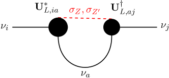
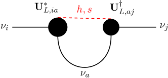
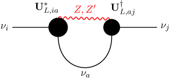
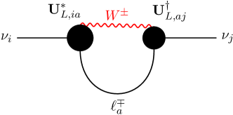
Figure 1: One-loop graphs contributing to the neutrino self energy. Top left: Goldstone boson contribution. Top right: scalar contribution. Bottom left: neutral gauge boson contribution. Bottom right: charged gauge boson contribution. Note that $W$ boson loop does not contribute to the matrix B_L.

III.2 Contributions with neutral gauge bosons in the loop

The contribution of the neutral gauge boson $V$ is

$$\Big{(}B_{L}^{V}(M_{V},\{m_{a}\};\xi_{V})\Big{)}_{ij}P_{L}=\mathrm{i}\int\!\frac{\mathrm{d}^{d}\ell}{(2\pi)^{d}}\sum_{a=1}^{6}\Gamma^{\mu}_{V\nu_{i}\nu_{a}}\frac{\not{p}-\not{\ell}+m_{a}}{(p-\ell)^{2}-m_{a}^{2}}\Gamma^{\nu}_{V\nu_{a}\nu_{j}}P_{\mu\nu}(\ell,M_{V}^{2};\xi_{V})$$ (III.8)

where $\xi_{V}$ is the gauge parameter and

$$P_{\mu\nu}(\ell,M_{V}^{2};\xi_{V})=\frac{g_{\mu\nu}}{\ell^{2}-M_{V}^{2}}-(1-\xi_{V})\frac{\ell_{\mu}\ell_{\nu}}{(\ell^{2}-M_{V}^{2})(\ell^{2}-\xi_{V}M_{V}^{2})}\,.$$ (III.9)

Introducing the $6\times 6$ matrix

$$\textbf{m}_{\ell}^{(n)}=\operatorname{diag}\left(\frac{m_{1}^{n}}{\ell^{2}-m_{1}^{2}},\dots,\frac{m_{6}^{n}}{\ell^{2}-m_{6}^{2}}\right),$$ (III.10)

and using the result of Appendix B, we obtain the following expression for a neutral vector boson in the loop:

$$\delta\textbf{M}_{L}^{V}=\mathrm{i}e^{2}\Big{(}C^{L}_{V\nu\nu}-C^{R}_{V\nu\nu}\Big{)}^{2}\int\!\frac{\mathrm{d}^{d}\ell}{(2\pi)^{d}}\textbf{U}_{L}^{*}\bigg{[}\frac{d\>\textbf{m}_{\ell}^{(1)}}{\ell^{2}-M_{V}^{2}}+\frac{\textbf{m}_{\ell}^{(3)}}{M_{V}^{2}}\left(\frac{1}{\ell^{2}-\xi_{V}M_{V}^{2}}-\frac{1}{\ell^{2}-M_{V}^{2}}\right)\bigg{]}\textbf{U}_{L}^{\dagger}.$$ (III.11)

III.3 Contributions with neutral Goldstone bosons in the loop

The contribution of the neutral Goldstone boson $\sigma_{V}$ ($V=1$ means the Goldstone boson belonging to the $Z$ field and $V=2$ refers to the $Z^{\prime}$ field) is

$$\Big{(}B_{L}^{\sigma_{V}}(m_{\sigma_{V}},\{m_{a}\};\xi_{V})\Big{)}_{ij}P_{L}=-\mathrm{i}\int\!\frac{\mathrm{d}^{d}\ell}{(2\pi)^{d}}\sum_{a=1}^{6}{\mbox{\boldmath$\Gamma$}}_{\sigma_{V}\nu_{i}\nu_{a}}\frac{m_{a}}{\ell^{2}-m_{a}^{2}}{\mbox{\boldmath$\Gamma$}}_{\sigma_{V}\nu_{a}\nu_{j}}\frac{1}{\ell^{2}-\xi_{V}M^{2}_{V}}\,.$$ (III.12)

Using the matrix notation, we can write

$$\textbf{U}_{L}^{*}\textbf{B}_{L}^{\sigma_{V}}(0)\textbf{U}_{L}^{\dagger}P_{L}=-\mathrm{i}\int\!\frac{\mathrm{d}^{d}\ell}{(2\pi)^{d}}\textbf{U}_{L}^{*}{\mbox{\boldmath$\Gamma$}}_{\sigma_{V}\nu\nu}\textbf{m}_{\ell}^{(1)}{\mbox{\boldmath$\Gamma$}}_{\sigma_{V}\nu\nu}\textbf{U}_{L}^{\dagger}\frac{1}{\ell^{2}-\xi_{V}M^{2}_{V}}\,.$$ (III.13)

Substituting the vertex functions of Eq. (II.40) and employing the matrix relations in Eqs. (A.2) and (A.5), we obtain the correction to the mass matrix as

$$\delta\textbf{M}_{L}^{\sigma_{V}}=-\mathrm{i}\int\!\frac{\mathrm{d}^{d}\ell}{(2\pi)^{d}}\textbf{U}_{L}^{*}\textbf{M}\textbf{m}_{\ell}^{(1)}\textbf{M}\textbf{U}_{L}^{\dagger}\left(\frac{(\textbf{Z}_{\rm G})_{V1}}{v}\right)^{2}\frac{1}{\ell^{2}-\xi_{V}M^{2}_{V}}\,.$$ (III.14)

We now substitute $\textbf{M}\textbf{m}_{\ell}^{(1)}\textbf{M}=\textbf{m}_{\ell}^{(3)}$ and using Eq. (II.30), we obtain

$$\delta\textbf{M}_{L}^{\sigma_{V}}=-\mathrm{i}e^{2}\Big{(}C^{L}_{V\nu\nu}-C^{R}_{V\nu\nu}\Big{)}^{2}\int\!\frac{\mathrm{d}^{d}\ell}{(2\pi)^{d}}\textbf{U}_{L}^{*}\frac{\textbf{m}_{\ell}^{(3)}}{M_{V}^{2}}\textbf{U}_{L}^{\dagger}\frac{1}{\ell^{2}-\xi_{V}M^{2}_{V}}\,.$$ (III.15)

III.4 Contributions with scalar bosons in the loop

The scalar – neutrino vertex is very similar to the Goldstone boson neutrino vertex, so the contribution with a scalar boson $S_{k}$ in the loop can be written immediately in analogy with Eq. (III.14):

$$\begin{split}\delta\textbf{M}_{L}^{S_{k}}&=\mathrm{i}\int\!\frac{\mathrm{d}^{d}\ell}{(2\pi)^{d}}\textbf{U}_{L}^{*}\textbf{M}\textbf{m}_{\ell}^{(1)}\textbf{M}\textbf{U}_{L}^{\dagger}\left(\frac{(\textbf{Z}_{S})_{k1}}{v}\right)^{2}\frac{1}{\ell^{2}-M^{2}_{S_{k}}}\\ &=\mathrm{i}\left(\frac{(\textbf{Z}_{S})_{k1}}{v}\right)^{2}\int\!\frac{\mathrm{d}^{d}\ell}{(2\pi)^{d}}\textbf{U}_{L}^{*}\textbf{m}_{\ell}^{(3)}\textbf{U}_{L}^{\dagger}\frac{1}{\ell^{2}-M^{2}_{S_{k}}}\,.\end{split}$$ (III.16)

III.5 The complete one-loop mass correction

Combining Eqs. (III.11), (III.15) and (III.16), we find that that the gauge-dependent pieces of the vector boson contribution cancel exactly with the Goldstone boson contribution, and obtain

$$\begin{split}\delta\textbf{M}_{L}&=\sum\limits_{V=Z,Z^{\prime}}\left(\delta\textbf{M}_{L}^{V}+\delta\textbf{M}_{L}^{\sigma_{V}}\right)+\sum\limits_{k=1,2}\delta\textbf{M}_{L}^{S_{k}}\\ &=\sum\limits_{V=Z,Z^{\prime}}\mathrm{i}e^{2}\Big{(}C^{L}_{V\nu\nu}-C^{R}_{V\nu\nu}\Big{)}^{2}\int\!\frac{\mathrm{d}^{d}\ell}{(2\pi)^{d}}\textbf{U}_{L}^{*}\bigg{[}\frac{d\>\textbf{m}_{\ell}^{(1)}}{\ell^{2}-M_{V}^{2}}-\frac{\textbf{m}_{\ell}^{(3)}}{M_{V}^{2}}\frac{1}{\ell^{2}-M_{V}^{2}}\bigg{]}\textbf{U}_{L}^{\dagger}\\ &\quad+\sum\limits_{k=1,2}\mathrm{i}\left(\frac{(\textbf{Z}_{S})_{k1}}{v}\right)^{2}\int\!\frac{\mathrm{d}^{d}\ell}{(2\pi)^{d}}\textbf{U}_{L}^{*}\frac{\textbf{m}_{\ell}^{(3)}}{\ell^{2}-M^{2}_{S_{k}}}\textbf{U}_{L}^{\dagger}\,.\end{split}$$ (III.17)

Introducing the integral

$$I_{0}(M^{2},m_{a}^{2};\mu^{2},\epsilon)=\mu^{2\epsilon}\int\frac{\mathrm{d}^{d}\ell}{(2\pi)^{d}}\frac{1}{(\ell^{2}-M^{2})(\ell^{2}-m_{a}^{2})}\,,$$ (III.18)

the matrix $\textbf{I}^{(n)}$ with elements

$$\textbf{I}^{(n)}_{ij}(M^{2})=\mathrm{i}\sum\limits_{a=1}^{6}(\textbf{U}_{L}^{*})_{ia}m_{a}^{n}(\textbf{U}_{L}^{\dagger})_{aj}I_{0}(M^{2},m_{a}^{2};\mu^{2},\epsilon)\,,$$ (III.19)

and using the relations (II.30) allows us to recast Eq. (III.17) into a neatly condensed form

$$\delta\textbf{M}_{L} =\sum\limits_{k=1,2}\left\{\left(\frac{(\textbf{Z}_{\rm G})_{k1}}{v}\right)^{2}\left(dM_{V_{k}}^{2}\textbf{I}^{(1)}(M_{V_{k}}^{2})-\textbf{I}^{(3)}(M_{V_{k}}^{2})\right)+\left(\frac{(\textbf{Z}_{S})_{k1}}{v}\right)^{2}\textbf{I}^{(3)}(M_{S_{k}}^{2})\right\}$$ (III.20)

with $V_{1}=Z$ and $V_{2}=Z^{\prime}$. In Eq. (III.18) $2\epsilon=d-4$ and $\mu$ is the regularization scale.

III.6 Finiteness and scale independence of $\delta\textbf{M}_{L}$

We show here that the one loop mass correction $\delta\textbf{M}_{L}$ is finite and independent of the scale $\mu$. Evaluating the integral (III.18) yields

$$I_{0}(M^{2},m^{2};\mu^{2},\epsilon) =I^{(\mathrm{s})}_{0}(\epsilon)+I^{(\mathrm{f})}_{0}\left(\frac{m^{2}}{M^{2}},\frac{\mu^{2}}{M^{2}}\right)+\mathrm{O}(\epsilon)$$ (III.21)

where ‘s’ stands for the singular and ‘f’ for the finite functions

$$I^{(\mathrm{s})}_{0}(\epsilon)=\frac{\mathrm{i}}{16\pi^{2}}\left(\frac{1}{\epsilon}-\gamma_{\mathrm{E}}+\ln 4\pi+1\right) ,\quad I^{(\mathrm{f})}_{0}(x,x_{\mu})=\frac{\mathrm{i}}{16\pi^{2}}\left(\frac{x\ln x}{1-x}+\ln x_{\mu}\right).$$ (III.22)

with $\gamma_{\mathrm{E}}\simeq 0.5722$ being the Euler-Mascheroni constant. It is also convenient to split the matrix (III.19) in a similar fashion

$$\textbf{I}^{(n)}(M^{2})=\textbf{I}^{(\mathrm{s},n)}+\textbf{I}^{(\mathrm{f},n)}(M^{2})$$ (III.23)

such that

$$\textbf{I}^{(\mathrm{s},n)}=\mathrm{i}\textbf{U}_{L}^{*}\textbf{M}^{n}\textbf{U}_{L}^{\dagger}I^{(\mathrm{s},n)}_{0}\,,\quad\Big{(}\textbf{I}^{(\mathrm{f},n)}(M^{2})\Big{)}_{ij}=\mathrm{i}\sum_{a=1}^{6}(\textbf{U}_{L}^{*})_{ia}m_{a}^{n}(\textbf{U}_{L}^{\dagger})_{aj}I^{(\mathrm{f},n)}_{0}\left(\frac{m_{a}^{2}}{M^{2}},\frac{\mu^{2}}{M^{2}}\right).$$ (III.24)

Then the one-loop correction to the mass matrix of the light neutrinos can also be decomposed as

$$\delta\textbf{M}_{L}=\delta\textbf{M}^{(\mathrm{s})}_{L}+\delta\textbf{M}^{(\mathrm{f})}_{L}+\mathrm{O}(\epsilon)$$ (III.25)

where

$$\delta\textbf{M}^{(\mathrm{s})}_{L} =\sum_{k=1,2}\left[dM_{V_{k}}^{2}\left(\frac{(\textbf{Z}_{\rm G})_{k1}}{v}\right)^{2}\textbf{I}^{(\mathrm{s},1)}+\frac{(\textbf{Z}_{S})^{2}_{k1}-(\textbf{Z}_{\rm G})^{2}_{k1}}{v^{2}}\textbf{I}^{(\mathrm{s},3)}\right]$$ (III.26)

and

$$\delta\textbf{M}^{(\mathrm{f})}_{L} =\sum\limits_{k=1,2}\left[\left(\frac{(\textbf{Z}_{\rm G})_{k1}}{v}\right)^{2}\left(dM_{V_{k}}^{2}\textbf{I}^{(\mathrm{f},1)}(M_{V_{k}}^{2})-\textbf{I}^{(\mathrm{f},3)}(M_{V_{k}}^{2})\right)+\left(\frac{(\textbf{Z}_{S})_{k1}}{v}\right)^{2}\textbf{I}^{(\mathrm{f},3)}(M_{S_{k}}^{2})\right].$$ (III.27)

In order to prove that $\delta\textbf{M}_{L}$ is finite, one has to show that $\delta\textbf{M}^{(\mathrm{s})}_{L}$ is free from $\epsilon$ poles. We prove that it in fact vanishes because the matrix $\textbf{I}^{(\mathrm{s},1)}$ is zero matrix due to the identity (A.5), while the coefficient in the second term cancels because the matrices Z_S and Z_G are orthogonal, so

$$\sum_{k=1}^{2}(\textbf{Z}_{S})_{k1}^{2}-\sum_{k=1}^{2}(\textbf{Z}_{G})_{k1}^{2}=0\,.$$ (III.28)

Hence the mass independent terms, including the divergent pieces of the light neutrino one-loop mass correction cancel, and we can set $\epsilon=0$, which yields $\delta\textbf{M}_{L}=\delta\textbf{M}^{(\mathrm{f})}_{L}$. Furthermore, the terms depending on the regularization scale in $\delta\textbf{M}^{(\mathrm{f})}_{L}$ cancel in an identical way as the second term does in $\delta\textbf{M}^{(\mathrm{s})}_{L}$ (using Eq. (III.28)).

The remaining finite terms give the final, regularization-scale independent and finite one-loop correction to the light neutrinos as given in Eq. (III.4). It is the linear combination of the matrix valued function F given in Eq. (III.5) with different arguments and coefficients corresponding to the different one-loop contributions. The function F gives the mass correction corresponding to a one loop diagram, before coupling suppression; see Fig. 4 in Sect. IV for details where we shall also give a numerical estimate for its eigenvalues $\delta m^{\nu}_{i,0}$. It is well defined for any non-negative $x$ because

$$\lim\limits_{x\rightarrow 0}\frac{x\ln x}{1-x}=0\text{~{}~{}and~{}~{}}\lim\limits_{x\rightarrow 1}\frac{x\ln x}{1-x}=-1\,.$$ (III.29)

III.7 Generalization to arbitrary number of neutral bosons and neutrinos

Our predictions for the one-loop correction to the light neutrino mass matrix can easily be generalized to any number of $n_{V}$ massive neutral gauge bosons, $n_{S}$ neutral real scalars coupling to $n_{a}$ active and $n_{s}$ sterile neutrinos. Clearly, the matrix form of gauge-dependent parts in Eq. (III.11) and Eq. (III.15) is unchanged, and they cancel in the same way.

The correction without gauge parameters $\xi_{V}$ in Eq. (III.4) is straightforwardly generalized to a case where the sums go over an arbitrary positive integer $n_{V}$ and $n_{S}$.

The neutrino mass and mixing matrices with arbitrary $n_{a}$ and $n_{s}$ are written identically in the block form, differing only on the block shape: U_L is a $n_{a}\times(n_{a}+n_{s})$ matrix and U_R is a $n_{s}\times(n_{a}+n_{s})$ matrix. The finite correction derived in Eq. (III.4) is then immediately generalized to

$$\begin{split}\delta\textbf{M}_{L}=\frac{1}{16\pi^{2}}\left[3\sum_{k=1}^{n_{V}}(\textbf{Z}_{\rm G})_{k1}^{2}\frac{M^{2}_{V_{k}}}{v^{2}}\textbf{F}(M_{V_{k}}^{2})+\sum_{k=1}^{n_{S}}(\textbf{Z}_{\rm S})_{k1}^{2}\frac{M^{2}_{S_{k}}}{v^{2}}\textbf{F}(M_{S_{k}}^{2})\right]\end{split}$$ (III.30)

where the upper limit in the summation in the matrix F is $n_{a}+n_{s}$. The factor 3 in front of the first term in the bracket of Eq. (III.30) stems from the three polarization states of the propagating massive neutral gauge bosons. The corresponding factor is of course one in the case of the scalars. This formula is also independent of the new U(1) charge assignments.

IV Numerical estimate of the corrections

We are now ready to estimate the order of magnitude of the corrections. We assume large mixing in the scalar sector: $\theta_{S}=\mathrm{O}(1)$. The $Z^{\prime}$ mass and mixing angle $\theta_{G}$ are fixed by the gauge couplings $g_{y}^{\prime}=\gamma_{y}^{\prime}g_{L}$ and $g_{z}^{\prime}$ and ratio of VEVs, $\tan\beta\equiv w/v$. We plot their magnitudes in Fig. 2, scanning the parameters $g_{y}^{\prime},g_{z}^{\prime}\in[10^{-6},1]$ and for $w=100,750$ GeV. Note that larger $\tan\beta$ corresponds to a larger Goldstone angle. Smaller $\tan\beta$ distorts the $M_{Z^{\prime}}$ contours so that the same $Z^{\prime}$ mass can be achieved with larger gauge couplings $g_{y}^{\prime}$ and $g_{z}^{\prime}$ compared to large $\tan\beta$. In addition, we set $M_{s}/v=\mathrm{O}(1)$, that is, only the mass of the $Z^{\prime}$ boson is free, and may be far from electroweak scale. The relevant gauge couplings can then be estimated as from Fig. 2 after identifying the region in $(g_{y}^{\prime},g_{z}^{\prime})$ plane corresponding to $M_{Z^{\prime}}\in[20,200]$ MeV, which is the relevant mass region for the super-weak model to reproduce the dark matter relic density, allowed by experimental constraints [29].

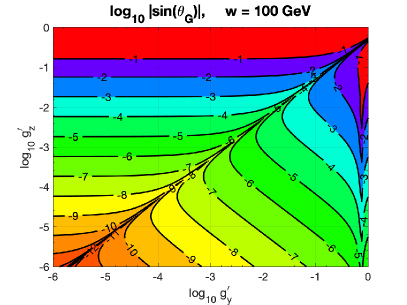
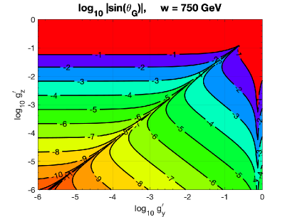
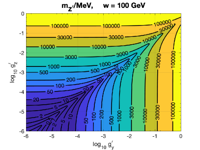
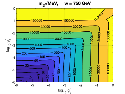
Figure 2: Absolute values of $\sin\theta_{G}$ (top) and mass of $Z^{\prime}$ boson (bottom) in logarithmic $(g_{y}^{\prime},g_{z}^{\prime})$ plane. For $\theta_{G}$ the contour labels $n$ correspond to value $10^{n}$. Left plots: $w=100$ GeV; right plots: $w=750$ GeV.

Then we identify the order-of-magnitude estimate for $|\sin\theta_{G}|$ by comparing the regions relevant to the mass range of $M_{Z^{\prime}}$. For $w=100$ GeV, we have $|\sin\theta_{G}|<10^{-6}$, which we take as a conservative upper limit. Then the prefactors in gauge boson contributions to $\delta\textbf{M}_{L}$ are

$$e^{2}(C^{L}_{Z\nu\nu}-C^{R}_{Z\nu\nu})^{2}=\cos^{2}\theta_{G}\frac{M_{Z}^{2}}{v^{2}}\sim\mathrm{O}(10^{-1})$$ (IV.1)

and

$$e^{2}(C^{L}_{Z^{\prime}\nu\nu}-C^{R}_{Z^{\prime}\nu\nu})^{2}=\sin^{2}\theta_{G}\frac{M_{Z^{\prime}}^{2}}{v^{2}}\sim\mathrm{O}(10^{-19})\times\left(\frac{M_{Z^{\prime}}}{100\,\text{MeV}}\right)^{2}.$$ (IV.2)

Then the numerical estimate for the total correction in Eq. (III.4) can be written as

$$(\delta\textbf{M}_{L})_{ij}<\mathrm{O}(10^{-7})\,\text{eV}+\mathrm{O}(10^{-21})\times\left(\frac{M_{Z^{\prime}}}{100\text{ MeV}}\right)^{2}\textbf{F}_{ij}(M_{Z^{\prime}}^{2})\,.$$ (IV.3)

The elements of the matrix F are plotted as a function of the mass of the boson of the loop $m_{\rm loop}$ in Fig. 3 and the eigenvalues of the matrix corresponding to corrections to active neutrino species in Fig. 4. The eigenvalues of F themselves exceed the active neutrino tree-level masses, as the latter are at most about 10 eV for the MeV scale $Z^{\prime}$ boson. However, the coupling suppressions in Eq. (IV.3) are sufficient to tame the relative correction to the tree level mass below the per cent level. Assuming the active neutrino masses to be $\mathrm{O}(10^{-3})$ eV, a rough estimate for the relative correction to active neutrino masses is of $\mathrm{O}(10^{-4})$.

We may maximize the effect of $Z^{\prime}$ loop by allowing $Z^{\prime}$ mass to be free and setting large $|\sin\theta_{G}|=\mathrm{O}(10^{-1})$, which is obtained when $g_{y}^{\prime}$ and $g_{z}^{\prime}$ are O($10^{-1}$). This corresponds to $M_{Z^{\prime}}=\mathrm{O}(M_{Z})$, which is of course, excluded. Yet, even in this case, the correction from $Z$ and $Z^{\prime}$ loops are small, have the same order of magnitude, $\mathrm{O}(10^{-7})$ eV. Thus, the individual contributions from BSM loops cannot be significantly larger than the SM contributions.

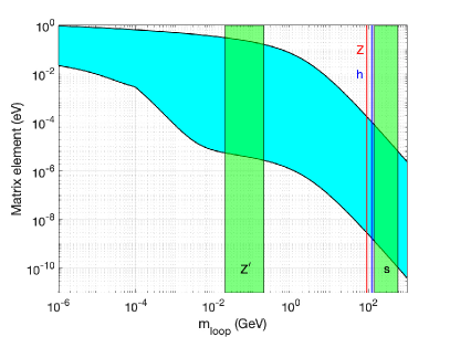
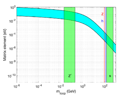
Figure 3: Matrix elements F_ij as a function of the mass $m_{\text{loop}}$ of the boson in the loop are confined to the blue band, assuming normal neutrino mass hierarchy. We have highlighted with vertical bands the relevant mass regions where the masses of the bosons in the loop lie. The scalar $s$ is required to have mass between 144 and 558 GeV requiring stability of the vacuum [38]. Left plot: $m_{1}^{\text{tree}}=0.01$ eV, $m_{4}^{\text{tree}}=30$ keV, $m_{5}^{\text{tree}}\approx m_{6}^{\text{tree}}=2.5$ GeV; right plot: $m_{1}^{\text{tree}}=0.001$ eV, $m_{4}^{\text{tree}}=7.1$ keV, $m_{5}^{\text{tree}}\approx m_{6}^{\text{tree}}=3.0$ GeV.

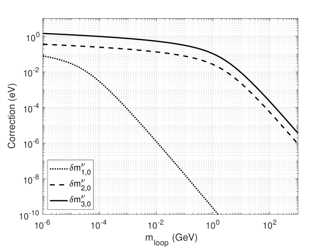
Figure 4: Eigenvalues of the matrix F as a function of the mass of the boson in the loop $m_{\text{loop}}$, assuming $m_{1}^{\text{tree}}=0.01$ eV, $m_{4}^{\text{tree}}=30$ keV, $m_{5}^{\text{tree}}\approx m_{6}^{\text{tree}}=2.5$ GeV, and normal neutrino mass hierarchy.

V Conclusions

In this paper, we have computed the one-loop corrections to the mass matrix of the active neutrinos in a gauged U(1) extension of the standard model of particle interactions. The field content of the model consists of a new complex scalar field and three right-handed neutrinos—sterile under the standard model interactions—in addition to the fields in the standard model. The neutrino masses are generated by Dirac and Majorana type Yukawa terms, which after spontaneous symmetry breaking of both scalar fields give rise to neutrino masses in the way of the type I see-saw mass generation. We used $R_{\xi}$ gauge and have shown that the one-loop corrections are (i) independent of the gauge fixing parameters, (ii) finite and (iii) independent of the regularization scale. We also demonstrated how the formula for the one-loop mass corrections can be generalized to the case of arbitrary number of new U(1) groups, complex scalars and right-handed neutrinos.

We have provided a numerical estimate of the size of the mass corrections in the context of the super-weak model, in which the new neutral gauge boson $Z^{\prime}$ is much lighter than the $Z$ boson of the standard model. We have found that in the mass range of $M_{Z^{\prime}}\in[20,200]$ MeV, motivated by a possible explanation of the relic density of dark matter in the Universe, the relative mass corrections to the tree-level mass matrix elements do not exceed the per mill level. Hence the model is stable against higher-order corrections in the neutrino sector, which motivates further studies to explore the viable parameter space of the model regarding the mixings between the active and sterile neutrinos [28].

Acknowledgments

We are grateful to Josu Hernández-García for discussions on this project. This work was supported by grant K 125105 of the National Research, Development and Innovation Fund in Hungary.

Appendix A Some properties of neutrino mass and mixing matrices

In this appendix, we derive some useful relations among the neutrino mass and mixing matrices. The matrix U that diagonalizes the neutrino mass matrix is unitary, hence

$$\textbf{UU}^{\dagger}=\binom{\textbf{U}_{L}}{\textbf{U}_{R}^{*}}(\textbf{U}_{L}^{\dagger},\textbf{U}_{R}^{T})=\begin{pmatrix}\textbf{U}_{L}\textbf{U}_{L}^{\dagger}&\textbf{U}_{L}\textbf{U}_{R}^{T}\\ \textbf{U}_{R}^{*}\textbf{U}_{L}^{\dagger}&\textbf{U}_{R}^{*}\textbf{U}_{R}^{T}\end{pmatrix}=\begin{pmatrix}{\mbox{\boldmath$1$}}_{3}&\textbf{0}_{3}\\ \textbf{0}_{3}&{\mbox{\boldmath$1$}}_{3}\end{pmatrix},$$ (A.1)

from which we obtain the following important relations:

$$\textbf{U}_{L}\textbf{U}_{L}^{\dagger}={\mbox{\boldmath$1$}}_{3}\,,\quad\textbf{U}_{R}\textbf{U}_{R}^{\dagger}={\mbox{\boldmath$1$}}_{3}$$ (A.2)

and

$$\textbf{U}_{L}\textbf{U}_{R}^{T}=\textbf{U}_{R}^{*}\textbf{U}_{L}^{\dagger}=\textbf{0}_{3}$$ (A.3)

where ${\mbox{\boldmath$1$}}_{n}$ denotes the $n\times n$ unit matrix. The second unitarity conditions gives

$$\textbf{U}^{\dagger}\textbf{U}=(\textbf{U}_{L}^{\dagger},\textbf{U}_{R}^{T})\binom{\textbf{U}_{L}}{\textbf{U}_{R}^{*}}=\textbf{U}_{L}^{\dagger}\textbf{U}_{L}+\textbf{U}_{R}^{T}\textbf{U}_{R}^{*}={\mbox{\boldmath$1$}}_{6}\,.$$ (A.4)

Using Eq. (II.35) we derive

$$\textbf{U}_{L}^{*}\textbf{M}\textbf{U}_{L}^{\dagger} =\textbf{U}_{L}^{*}(\textbf{U}_{L}^{T},\textbf{U}_{R}^{\dagger})\begin{pmatrix}\textbf{0}_{3}&\textbf{M}_{D}^{T}\\ \textbf{M}_{D}&\textbf{M}_{N}\end{pmatrix}\binom{\textbf{U}_{L}}{\textbf{U}_{R}^{*}}\textbf{U}_{L}^{\dagger}$$

$$=\textbf{U}_{L}^{*}\textbf{U}_{L}^{T}\textbf{M}_{D}\textbf{U}_{R}^{*}\textbf{U}_{L}^{\dagger}+\textbf{U}_{L}^{*}\textbf{U}_{R}^{\dagger}\textbf{M}_{D}\textbf{U}_{L}\textbf{U}_{L}^{\dagger}+\textbf{U}_{L}^{T}\textbf{U}_{R}^{\dagger}\textbf{M}_{N}\textbf{U}_{R}^{*}\textbf{U}_{L}^{\dagger}\,,$$

and then with relations in Eq. (A.3) we obtain

$$\textbf{U}_{L}^{*}\textbf{M}\textbf{U}_{L}^{\dagger}={\mbox{\boldmath$0$}}_{3}\,.$$ (A.5)

Analogous calculations yield

$$\textbf{U}_{R}\textbf{M}\textbf{U}_{L}^{\dagger}=\textbf{M}_{D}\,.$$ (A.6)

Multiplying Eq. (A.6) with $\textbf{U}_{R}^{\dagger}$ from the left and using Eq. (A.4), we find

$$\textbf{U}_{R}^{\dagger}\textbf{M}_{D}=\textbf{U}_{R}^{\dagger}\textbf{U}_{R}\textbf{M}\textbf{U}_{L}^{\dagger}=({\mbox{\boldmath$1$}}_{6}-\textbf{U}_{L}^{T}\textbf{U}_{L}^{*})\textbf{M}\textbf{U}_{L}^{\dagger}=\textbf{M}\textbf{U}_{L}^{\dagger}-\textbf{U}_{L}^{T}\textbf{U}_{L}^{*}\textbf{M}\textbf{U}_{L}^{\dagger}$$ (A.7)

where the last term vanishes by Eq. (A.5), so

$$\textbf{U}_{R}^{\dagger}\textbf{M}_{D}=\textbf{M}\textbf{U}_{L}^{\dagger}\,.$$ (A.8)

Finally,

$$\textbf{U}_{R}\textbf{M}\textbf{U}_{R}^{T} =\textbf{U}_{R}(\textbf{U}_{L}^{T},\textbf{U}_{R}^{\dagger})\begin{pmatrix}\textbf{0}&\textbf{M}_{D}^{T}\\ \textbf{M}_{D}&\textbf{M}_{N}\end{pmatrix}\binom{\textbf{U}_{L}}{\textbf{U}_{R}^{*}}\textbf{U}_{R}^{T}$$

$$=\textbf{U}_{R}\Big{(}\textbf{U}_{L}^{T}\textbf{M}_{D}^{T}\textbf{U}_{R}^{*}+\textbf{U}_{R}^{\dagger}\textbf{M}_{D}\textbf{U}_{L}+\textbf{U}_{R}^{\dagger}\textbf{M}_{N}\textbf{U}_{R}^{*}\Big{)}\textbf{U}_{R}^{T}$$

Expanding the factors into the parenthesis, the first two terms give vanishing contribution by Eq. (A.4), while utilizing Eq. (A.2), the last one is simply $\textbf{M}_{N}$, so

$$\textbf{U}_{R}\textbf{M}\textbf{U}_{R}^{T}=\textbf{M}_{N}\,.$$ (A.9)

Now Eq. (A.4) allows us to derive

$$\textbf{U}_{R}^{\dagger}\textbf{M}_{N}=\textbf{U}_{R}^{\dagger}\textbf{U}_{R}\textbf{M}\textbf{U}_{R}^{T}=({\mbox{\boldmath$1$}}_{6}-\textbf{U}_{L}^{T}\textbf{U}_{L}^{*})\textbf{M}\textbf{U}_{R}^{T}=\textbf{M}\textbf{U}_{R}^{T}-\textbf{U}_{L}^{T}\textbf{U}_{L}^{*}\textbf{M}\textbf{U}_{R}^{T}\,.$$ (A.10)

where the second term on the right does not vanish this time.

Appendix B Evaluation of the vector boson exchange diagram

The vector boson exchange diagrams, shown in the bottom row of Fig. 1 contribute gauge-dependent terms to the neutrino self energy. In order to show that the gauge-dependent terms cancel once contributions from all particles are considered, it is useful to eliminate the loop momentum from the one loop integral corresponding to the vector boson exchange diagram. A decomposition to achieve this was used in Ref. [39], and we shall derive it here as well. In Ref. [40], Eq (4.4) contains the self energy:

$$\mathrm{i}\Sigma_{V}(p)=-\int\frac{d^{d}\ell}{(2\pi)^{d}}{\mbox{\boldmath$\Gamma$}}^{\mu\dagger}\textbf{P}(p-\ell){\mbox{\boldmath$\Gamma$}}^{\nu}P_{\mu\nu}(\ell,M_{V}^{2};\xi_{V}),$$ (B.1)

where the $6\times 6$ matrices are defined as follows. The matrix P is the fermion propagator, diagonal in the mass eigenstates,

$$\textbf{P}(p-\ell)=[(\cancel{p}-\cancel{\ell}){\mbox{\boldmath$1$}}-\textbf{M}]^{-1}\,,\text{~{}~{}while~{}~{}}{\mbox{\boldmath$\Gamma$}}^{\mu}=-\mathrm{i}e\gamma^{\mu}\textbf{A}\,,\text{~{}~{}with~{}~{}}\textbf{A}={\mbox{\boldmath$\Gamma$}}^{L}P_{L}+{\mbox{\boldmath$\Gamma$}}^{R}P_{R}.$$ (B.2)

In the following we shall write P for $\textbf{P}(p-\ell)$. The matrix A is self-adjoint, $\textbf{A}^{\dagger}=\textbf{A}$, and so is ${\mbox{\boldmath$\Gamma$}}^{L/R}$. We also introduce the abbreviation

$$\tilde{\textbf{A}}={\mbox{\boldmath$\Gamma$}}^{R}P_{L}+{\mbox{\boldmath$\Gamma$}}^{L}P_{R}\,,$$ (B.3)

which will simplify our calculations. In order to compute the loop integral easily containing the neutral vector boson propagator in the neutrino self-energy loop, in this Appendix we perform tensor reduction of the matrix product

$$\cancel{\ell}\textbf{A}^{\dagger}\textbf{P}\cancel{\ell}\textbf{A}$$ (B.4)

such that the numerator factor be at most linear in the loop momentum $\ell$.

When the fermion momentum $p$ appears as $\cancel{p}$ at the extreme left or right of the expression, it satisfies the Dirac equation $\cancel{p}{\mbox{\boldmath$1$}}_{6}=\textbf{M}$ (both Dirac and Majorana fermions do so), thus we can replace formally $\cancel{p}$ with M. Let us first write the identity

$$\cancel{\ell}\textbf{A}^{\dagger} =(\cancel{\ell}-\cancel{p}+\textbf{M})\textbf{A}^{\dagger}=\textbf{MA}^{\dagger}-(\cancel{p}-\cancel{\ell})\textbf{A}^{\dagger}.$$ (B.5)

The chiral coupling matrix A anticommutes with the Dirac matrices $\gamma_{\mu}$, hence

$$\cancel{\ell}\textbf{A}^{\dagger}=\textbf{M}\textbf{A}^{\dagger}-\tilde{\textbf{A}}^{\dagger}\Big{(}(\cancel{p}-\cancel{\ell}){\mbox{\boldmath$1$}}-\textbf{M}+\textbf{M}\Big{)} =\textbf{M}\textbf{A}^{\dagger}-\tilde{\textbf{A}}^{\dagger}\textbf{P}^{-1}-\tilde{\textbf{A}}^{\dagger}\textbf{M}\,,$$ (B.6)

and similarly,

$$\textbf{P}\cancel{\ell}\textbf{A}=-\textbf{A}-\textbf{P}\textbf{MA}+\textbf{P}\tilde{\textbf{A}}\textbf{M}\,.$$ (B.7)

Multiplying Eqs. (B.6) and (B.7), we obtain the expression (B.4), and its expansion yields

$$\begin{split}\cancel{\ell}\textbf{A}^{\dagger}\textbf{P}\cancel{\ell}\textbf{A}=&-\textbf{MA}^{\dagger}\textbf{A}-\textbf{MA}^{\dagger}\textbf{P}\textbf{MA}+\textbf{MA}^{\dagger}\textbf{P}\textbf{AM}+\tilde{\textbf{A}}^{\dagger}\textbf{P}^{-1}\textbf{A}\\ &+\tilde{\textbf{A}}^{\dagger}\textbf{MA}-\tilde{\textbf{A}}^{\dagger}\tilde{\textbf{A}}\textbf{M}+\tilde{\textbf{A}}^{\dagger}\textbf{MA}+\tilde{\textbf{A}}^{\dagger}\textbf{M}\textbf{P}\textbf{MA}-\tilde{\textbf{A}}^{\dagger}\textbf{M}\textbf{P}\tilde{\textbf{A}}\textbf{M}\,.\end{split}$$ (B.8)

Using that $\cancel{p}\textbf{A}=\tilde{\textbf{A}}\cancel{p}$, the fourth term can rearranged as

$$\begin{split}\tilde{\textbf{A}}^{\dagger}\textbf{P}^{-1}\textbf{A}&=\tilde{\textbf{A}}^{\dagger}\Big{(}(\cancel{p}-\cancel{\ell})\textbf{1}-\textbf{M}\Big{)}\textbf{A}=\frac{1}{2}\tilde{\textbf{A}}^{\dagger}\cancel{p}\textbf{A}+\frac{1}{2}\tilde{\textbf{A}}^{\dagger}\cancel{p}\textbf{A}-\tilde{\textbf{A}}^{\dagger}\cancel{\ell}\textbf{A}-\tilde{\textbf{A}}^{\dagger}\textbf{MA}\\ &=\frac{1}{2}\cancel{p}\textbf{A}^{\dagger}\textbf{A}+\frac{1}{2}\tilde{\textbf{A}}^{\dagger}\tilde{\textbf{A}}\cancel{p}-\tilde{\textbf{A}}^{\dagger}\cancel{\ell}\textbf{A}-\tilde{\textbf{A}}^{\dagger}\textbf{MA}\end{split}$$ (B.9)

The $\cancel{p}$ is on extreme left and right, hence can be replaced with M, giving

$$\tilde{\textbf{A}}^{\dagger}\textbf{P}^{-1}\textbf{A}=\frac{1}{2}\textbf{M}\textbf{A}^{\dagger}\textbf{A}+\frac{1}{2}\tilde{\textbf{A}}^{\dagger}\tilde{\textbf{A}}\textbf{M}-\tilde{\textbf{A}}^{\dagger}\cancel{\ell}\textbf{A}-\tilde{\textbf{A}}^{\dagger}\textbf{MA}\,.$$ (B.10)

Substituting Eq. (B.10) into Eq. (B.8), we obtain

$$\cancel{\ell}\textbf{A}^{\dagger}\textbf{P}\cancel{\ell}\textbf{A}=\textbf{M}_{0}+\textbf{M}_{1}+\textbf{M}_{2}$$ (B.11)

where we introduced the abbreviations

$$\begin{split}\textbf{M}_{0}&=-\tilde{\textbf{A}}^{\dagger}\cancel{\ell}\textbf{A}\,,\\ \textbf{M}_{1}&=-\frac{1}{2}\textbf{M}\textbf{A}^{\dagger}\textbf{A}-\frac{1}{2}\tilde{\textbf{A}}^{\dagger}\tilde{\textbf{A}}\textbf{M}+\tilde{\textbf{A}}^{\dagger}\textbf{MA}\end{split}$$ (B.12)

and

$$\begin{split}\textbf{M}_{2}&=-\textbf{MA}^{\dagger}\textbf{P}\textbf{MA}+\textbf{MA}^{\dagger}\textbf{P}\tilde{\textbf{A}}\textbf{M}+\tilde{\textbf{A}}^{\dagger}\textbf{M}\textbf{P}\textbf{MA}-\tilde{\textbf{A}}^{\dagger}\textbf{M}\textbf{P}\tilde{\textbf{A}}\textbf{M}\\ &=(\textbf{MA}^{\dagger}-\tilde{\textbf{A}}^{\dagger}\textbf{M})\textbf{P}(\tilde{\textbf{A}}\textbf{M}-\textbf{MA})\,,\end{split}$$ (B.13)

which correspond to constant, linear and quadratic terms in the neutrino mass matrix M. We now discuss the contribution from each term in Eq. (B.11) separately.

The first, constant term gives vanishing contribution to the loop integral as it is odd in the loop momentum. The other two terms can be decomposed into left and right chiral pieces:

$$\textbf{M}_{i}=\textbf{M}_{i}^{L}P_{L}+\textbf{M}_{i}^{R}P_{R}\,.$$ (B.14)

Our goal is to compute the one-loop correction (III.7) to the tree-level mass matrix of the light neutrinos. In order to obtain it, one sandwiches the left handed pieces $\textbf{M}_{i}^{L}$ between the matrices $\textbf{U}_{L}^{*}$ and $\textbf{U}_{L}^{\dagger}$. Using the properties of the neutrino mixing matrices of Appendix A, we immediately see that

$$\textbf{U}_{L}^{*}\textbf{M}_{1}^{L}\textbf{U}_{L}^{\dagger}=0\,,$$ (B.15)

while lengthy computations yield

$$\begin{split}\textbf{U}_{L}^{*}\textbf{M}_{2}^{L}\textbf{U}_{L}^{\dagger}=&-(C^{L}_{V\nu\nu}-C^{R}_{V\nu\nu})^{2}\textbf{U}_{L}^{*}\textbf{M}\textbf{P}\textbf{MU}_{L}^{\dagger}\\ &+\text{terms that do not contribute to {\bf B}}_{L}(0)\,.\end{split}$$ (B.16)

Here we outline the steps needed to reach Eq. (B.16).

Firstly, in order to find the left-chiral part $\textbf{M}_{2}^{L}$, we substitute A and $\tilde{\textbf{A}}$ into Eq. (B.13). We write the denominator of the fermion propagator as

$$(\textbf{P})_{ij}=\delta_{ij}\frac{\not{p}-\not{\ell}+m_{i}}{(p-\ell)^{2}-m_{i}^{2}}$$ (B.17)

and use the following relations for the Dirac projectors:

$$P_{L/R}(\not{q}+m)P_{L/R}=mP_{L/R}\,,\quad P_{L/R}(\not{q}+m)P_{R/L}=\not{q}P_{R/L}\,,$$ (B.18)

valid for any momentum $q$ and mass $m$. Hence

$$\begin{split}P_{L/R}(\textbf{P})_{ij}P_{L/R}&=\left((\textbf{P})_{ij}-\delta_{ij}\frac{\not{p}-\not{\ell}}{(p-\ell)^{2}-m_{i}^{2}}\right)P_{L/R}\,,\\ P_{L/R}(\textbf{P})_{ij}P_{R/L}&=\delta_{ij}\frac{\not{p}-\not{\ell}}{(p-\ell)^{2}-m_{i}^{2}}P_{R/L}\,,\end{split}$$ (B.19)

and therefore, we obtain

$$\textbf{M}_{2}^{L}=-\textbf{M}{\mbox{\boldmath$\Gamma$}}^{L\dagger}\textbf{P}\textbf{M}{\mbox{\boldmath$\Gamma$}}^{L}+\textbf{M}{\mbox{\boldmath$\Gamma$}}^{L\dagger}\textbf{P}{\mbox{\boldmath$\Gamma$}}^{R}\textbf{M}+{\mbox{\boldmath$\Gamma$}}^{R\dagger}\textbf{M}\textbf{P}\textbf{M}{\mbox{\boldmath$\Gamma$}}^{L}-{\mbox{\boldmath$\Gamma$}}^{R\dagger}\textbf{M}\textbf{P}{\mbox{\boldmath$\Gamma$}}^{R}\textbf{M}+\textbf{D}$$ (B.20)

where the last term is proportional to $(\not{p}-\not{\ell})$:

$$\textbf{D}=[\textbf{M}({\mbox{\boldmath$\Gamma$}}^{L\dagger}-{\mbox{\boldmath$\Gamma$}}^{R\dagger})-({\mbox{\boldmath$\Gamma$}}^{L\dagger}-{\mbox{\boldmath$\Gamma$}}^{R\dagger})\textbf{M})](\not{p}-\not{\ell})[(p-l)^{2}{\mbox{\boldmath$1$}}_{6}-\textbf{M}^{2}]^{-1}({\mbox{\boldmath$\Gamma$}}^{R}\textbf{M}-\textbf{M}{\mbox{\boldmath$\Gamma$}}^{L})\,.$$

Then using the matrix relations derived in Appendix A, we can compute the following identities:

$$\textbf{U}_{L}^{*}\textbf{M}{\mbox{\boldmath$\Gamma$}}^{L\dagger} =-C_{V\nu\nu}^{R}\textbf{U}_{L}^{*}\textbf{M}\,,\quad\textbf{U}_{L}^{*}{\mbox{\boldmath$\Gamma$}}^{R\,\dagger}=-C^{L}_{V\nu\nu}\textbf{U}_{L}^{*}\,,$$ (B.21)

$${\mbox{\boldmath$\Gamma$}}^{R}\textbf{MU}_{L}^{\dagger} =C^{R}_{V\nu\nu}\textbf{MU}_{L}^{\dagger}\,,\qquad\;{\mbox{\boldmath$\Gamma$}}^{L}\textbf{U}_{L}^{\dagger}=C^{L}_{V\nu\nu}\textbf{U}_{L}^{\dagger}\,.$$ (B.22)

Finally sandwiching Eq. (B.20) gives us

$$\begin{split}\textbf{U}_{L}^{*}\textbf{M}_{2}^{L}\textbf{U}_{L}^{\dagger}&=-(C^{L}_{V\nu\nu}-C^{R}_{V\nu\nu})^{2}\textbf{U}_{L}^{*}\textbf{M}\textbf{P}\textbf{MU}_{L}^{\dagger}+\textbf{U}_{L}^{*}\textbf{D}\textbf{U}_{L}^{\dagger}\,.\end{split}$$ (B.23)

As mentioned, the last term is proportional to $(\not{p}-\not{\ell})$, but only the term with $\not{\ell}$ contributes to $\textbf{B}_{L}(p=0)$. That piece, being an odd function of $\ell$, vanishes upon integration, which completes the proof of Eq. (B.16).

The charged vector bosons $W^{\pm}$ also contribute to the neutrino self-energy. The corresponding Feynman rules are

$${\mbox{\boldmath$\Gamma$}}^{\mu}_{W^{-}\bar{\ell}\nu}=-\mathrm{i}e\gamma^{\mu}{\mbox{\boldmath$\Gamma$}}^{L}_{W^{-}\bar{\ell}\nu}P_{L},\quad{\mbox{\boldmath$\Gamma$}}^{\mu}_{W^{+}\nu\ell}=-\mathrm{i}e\gamma^{\mu}{\mbox{\boldmath$\Gamma$}}^{L}_{W^{+}\nu\ell}P_{L}.$$ (B.24)

where

$${\mbox{\boldmath$\Gamma$}}^{L}_{W^{-}\bar{\ell}\nu}=C_{W\ell\nu}(\textbf{U}_{L}^{\ell}\textbf{U}_{L})_{ij}$$ (B.25)

with $\textbf{U}_{L}^{\ell}$ being the charged lepton mixing matrix and ${\mbox{\boldmath$\Gamma$}}^{L}_{W^{-}\bar{\ell}\nu}=({\mbox{\boldmath$\Gamma$}}^{L}_{W^{+}\nu\ell})^{\dagger}$. The charged vector boson contribution to (III.7) is proportional to $\textbf{U}_{L}^{*}\textbf{M}\textbf{U}_{L}^{\dagger}$, which vanishes identically as shown in Appendix A.

References

- [1] Y. Fukuda et al. Measurements of the solar neutrino flux from super-kamiokande’s first 300 days. Phys. Rev. Lett., 81:1158–1162, Aug 1998.
- [2] Q. R. Ahmad et al. Measurement of the rate of interactions produced by solar neutrinos at the sudbury neutrino observatory. Phys. Rev. Lett., 87:071301, Jul 2001.
- [3] H. Fritzsch, M. Gell-Mann, and P. Minkowski. Vectorlike weak currents and new elementary fermions. Physics Letters B, 59(3):256 – 260, 1975.
- [4] Peter Minkowski. at a Rate of One Out of Muon Decays? Phys. Lett., 67B:421–428, 1977.
- [5] Murray Gell-Mann, Pierre Ramond, and Richard Slansky. Complex Spinors and Unified Theories. Conf. Proc., C790927:315–321, 1979.
- [6] Tsutomu Yanagida. Horizontal symmetry and masses of neutrinos. Conf. Proc., C7902131:95–99, 1979.
- [7] Rabindra N. Mohapatra and Goran Senjanović. Neutrino mass and spontaneous parity nonconservation. Phys. Rev. Lett., 44:912–915, Apr 1980.
- [8] J. Schechter and J. W. F. Valle. Neutrino Masses in SU(2) U(1) Theories. Phys. Rev., D22:2227, 1980.
- [9] M. Magg and C. Wetterich. Neutrino Mass Problem and Gauge Hierarchy. Phys. Lett., 94B:61–64, 1980.
- [10] S. L. Glashow. The Future of Elementary Particle Physics. NATO Sci. Ser. B, 61:687, 1980.
- [11] B. Abi et al. Measurement of the Positive Muon Anomalous Magnetic Moment to 0.46 ppm. Phys. Rev. Lett., 126(14):141801, 2021.
- [12] A. A. Aguilar-Arevalo et al. Observation of a Significant Excess of Electron-Like Events in the MiniBooNE Short-Baseline Neutrino Experiment. 2018.
- [13] Ann E. Nelson and Jonathan Walsh. Short Baseline Neutrino Oscillations and a New Light Gauge Boson. Phys. Rev. D, 77:033001, 2008.
- [14] Julian Heeck and Werner Rodejohann. Gauged and different Muon Neutrino and Anti-Neutrino Oscillations: MINOS and beyond. J. Phys. G, 38:085005, 2011.
- [15] Ernest Ma. Gauged B - 3L(tau) and radiative neutrino masses. Phys. Lett. B, 433:74–81, 1998.
- [16] Ernest Ma, D. P. Roy, and Sourov Roy. Gauged L(mu) - L(tau) with large muon anomalous magnetic moment and the bimaximal mixing of neutrinos. Phys. Lett. B, 525:101–106, 2002.
- [17] Kento Asai. Predictions for the neutrino parameters in the minimal model extended by linear combination of U(1), U(1) and U(1)B-L gauge symmetries. Eur. Phys. J. C, 80(2):76, 2020.
- [18] Disha Bhatia, Sabyasachi Chakraborty, and Amol Dighe. Neutrino mixing and anomaly in U(1)X models: a bottom-up approach. JHEP, 03:117, 2017.
- [19] Rathin Adhikari, Jens Erler, and Ernest Ma. Seesaw Neutrino Mass and New U(1) Gauge Symmetry. Phys. Lett. B, 672:136–140, 2009.
- [20] Debasish Borah, Lopamudra Mukherjee, and Soumitra Nandi. Low scale U(1)X gauge symmetry as an origin of dark matter, neutrino mass and flavour anomalies. JHEP, 12:052, 2020.
- [21] D. Aristizabal Sierra and Carlos E. Yaguna. On the importance of the 1-loop finite corrections to seesaw neutrino masses. JHEP, 08:013, 2011.
- [22] J. Lopez-Pavon, S. Pascoli, and Chan-fai Wong. Can heavy neutrinos dominate neutrinoless double beta decay? Phys. Rev. D, 87(9):093007, 2013.
- [23] Walter Grimus and Luis Lavoura. One-loop corrections to the seesaw mechanism in the multi-Higgs-doublet standard model. Phys. Lett. B, 546:86–95, 2002.
- [24] W. Grimus and M. Löschner. Renormalization of the multi-Higgs-doublet Standard Model and one-loop lepton mass corrections. JHEP, 11:087, 2018.
- [25] Vytautas Dūdėnas and Thomas Gajdosik. Gauge dependence of tadpole and mass renormalization for a seesaw extended 2HDM. Phys. Rev. D, 98(3):035034, 2018.
- [26] Ansgar Denner, Laura Jenniches, Jean-Nicolas Lang, and Christian Sturm. Gauge-independent renormalization in the 2HDM. JHEP, 09:115, 2016.
- [27] Zoltán Trócsányi. Super-weak force and neutrino masses. Symmetry, 12(1):107, 2020.
- [28] Timo J. Kärkkäinen and Zoltán Trócsányi. prepared for submission.
- [29] Sho Iwamoto, Károly Seller, and Zoltán Trócsányi. Sterile neutrino dark matter in a U(1) extension of the standard model. 4 2021.
- [30] Zoltán Péli, István Nándori, and Zoltán Trócsányi. Particle physics model of curvaton inflation in a stable universe. Phys. Rev. D, 101(6):063533, 2020.
- [31] F. Staub. Sarah, 2012.
- [32] Florian Staub. From superpotential to model files for feynarts and calchep/comphep. Computer Physics Communications, 181(6):1077–1086, 2010.
- [33] Florian Staub. Automatic calculation of supersymmetric renormalization group equations and loop corrections. Computer Physics Communications, 182(3):808–833, 2011.
- [34] Florian Staub. Sarah 4: A tool for (not only susy) model builders. Computer Physics Communications, 185(6):1773–1790, 2014.
- [35] We present the model files in a separate file SuperWeak.zip.
- [36] Note the opposite sign convention for in this work and in Ref. [27] where this mixing angle was denoted as , so .
- [37] This matrix coincides with the unitary matrix used by SARAH.
- [38] Zoltán Péli and Zoltán Trócsányi. Stability of the vacuum as constraint on (1) extensions of the standard model. 2 2019.
- [39] Maximilian Löschner. Renormalization and one-loop corrections of lepton masses. PhD thesis, Vienna U., 2018.
- [40] Steven Weinberg. Perturbative Calculations of Symmetry Breaking. Phys. Rev. D, 7:2887–2910, 1973.