Late-time acceleration with a scalar field source: Observational constraints and statefinder diagnostics

Abstract

This article discusses a dark energy cosmological model in the standard theory of gravity - general relativity with a broad scalar field as a source. Exact solutions of Einstein’s field equations are derived by considering a particular form of deceleration parameter $q$, which shows a smooth transition from decelerated to accelerated phase in the evolution of the universe. The external datasets such as Hubble ($H(z)$) datasets, Supernovae (SN) datasets, and Baryonic Acoustic Oscillation (BAO) datasets are used for constraining the model par parameters appearing in the functional form of $q$. The transition redshift is obtained at $z_{t}=0.67_{-0.36}^{+0.26}$ for the combined data set ($H(z)+SN+BAO$), where the model shows signature-flipping and is consistent with recent observations. Moreover, the present value of the deceleration parameter comes out to be $q_{0}=-0.50_{-0.11}^{+0.12}$ and the jerk parameter $j_{0}=-0.98_{-0.02}^{+0.06}$ (close to 1) for the combined datasets, which is compatible as per Planck2018 results. The analysis also constrains the omega value i.e., $\Omega_{m_{0}}\leq 0.269$ for the smooth evolution of the scalar field EoS parameter. It is seen that energy density is higher for the effective energy density of the matter field than energy density in the presence of a scalar field. The evolution of the physical and geometrical parameters is discussed in some details with the model parameters’ numerical constrained values. Moreover, we have performed the state-finder analysis to investigate the nature of dark energy.

I Introduction

Cosmological observations indicate that our universe is going through a phase of an accelerated expansion Riess ; Perlmutter , which is also supported by the recent SNe Ia observations SNIa , CMB observations CMB , BAO peak experiments BAO and $H(z)$ measurements Hz . These observations also indicate that the cosmological entity is responsible for the acceleration. In addition to that, this entity should also create an anti-gravitational effect to push the universe apart. The unknown force responsible for the accelerated expansion possessing a negative pressure is generally termed ”dark energy”(DE). According to the $\Lambda$CDM model, the best current measurement for dark energy is 69 percentage, i.e., $\frac{3}{4}$th of the total energy in the present-day observable universe. Since ordinary baryonic matter does not have such an equation of state, let alone to account for such a lion-share of the energy budget of the universe, several alternate scenarios have been proposed and investigatedalternate .

Since dark energy is mysterious and not much idea about its nature, several dark energy candidates have been proposed. Out of these various possible choices to study dark energy, Einstein’s cosmological constant ($\Lambda$) introduced in 1917, serves the best and simplest candidate, as described in the literature. This suggests that the repulsive nature of $\Lambda$ is responsible for accelerating the universe with the equation of state $\omega=-1$. However, this authentic candidate suffers from some long-standing cosmological constant problem and also the constant equation of state. As we know, the EoS parameter is the connection between energy density and pressure i.e. $\omega=\frac{p}{\rho}$. The EoS parameter is used to characterize the universe’s decelerated and accelerated expansion. It categorizes different phases of the universe as, If $\omega=\frac{1}{3}$, the model indicates the phase dominated by radiation, while $\omega=0$ represents the phase dominated by matter. In the current accelerated period of evolution, the quintessence period is shown by $-1<\omega\leq 0$ and the cosmological constant $\omega=-1$, i.e., the $\Lambda$CDM model and the phantom age by $\omega<-1$. The recent fine-tuning problem can be minimized by considering the equation of state as time-dependent. One such model having this property is the scalar field, also known as quintessence Sahni . The presence of scalar fields $\phi$ is predicted by several fundamental physics theories, encouraging to study the dynamic properties of scalar fields in cosmology. A wide range of scalar-field dark energy models has been suggested so far. Among several, these include quintessence, K-essence, tachyon, phantoms etc. Quintessence depends on scalar fields’ potential energy to contribute to the acceleration of the late time universe. The potential $V(\phi)$ has the property such that scalar fields are rotating down potential approach a common evolutionary path. For large values of $\phi$, the potential becomes flat, winding scalar fields to slow down, allowing the universe to accelerate. This ordinary scalar field model is a viable alternative that has a dynamical equation of state (EoS) wherein the EoS parameter $\omega$ ranges in between $-1/3$ to $-1$. A route to dark energy is also provided by Chaplygin gas AY/2001 which has a peculiar EoS and also phantom field Bamba/2012 for which $\omega$ crosses $-1$.

Implementing SN distance measurements Riess ; Perlmutter with baryon acoustic peak measurements in the power spectrum of cosmic microwave background(CMB) suggests that our universe is accelerating and composed predominantly of baryon, dark matter, and dark energy. The cosmic microwave background (CMB) is landmark proof of the universe’s Big Bang origin. Precise CMB measurements are essential to cosmology, as any proposed model of the universe must clarify this radiation. Current observational data is used to constrain the $f(z)$ models and describe distance-redshift relations. Here, $f(z)$ refers to constraining the $H(z)$ models. Nevertheless, given its role as a hypothesis, the $\Lambda$CDM model was immensely successful in explaining most cosmological observations. In addition to a moderately significant difference with broad angular scale CMB observations, $\Lambda$CDM provided an almost ideal match to measurements made by the Wilkinson Microwave Anisotropy probe (WMAP) satellite project mission. Even in parallel with corresponding observational data such as BAO surveys, Type Ia supernovae, and Hubble constant direct measurements. The Baryon Acoustic Oscillations (BAO) matter clustering provides a ‘standard ruler’ for length scale in cosmology the same way as supernovae offer a ‘standard candle’ for astronomical observations. There are different observational data also discussed in Valentino ; J.K.Singh : Cosmic microwave background radiation (CMB) acts as authentication of big bang theory, Sloan digital sky survey (SDSS), which provides a map of the distribution of the galaxy and encodes the existing variations in the universe, Baryon acoustic oscillations (BAO) Aghanim estimates large-scale structures in the universe that make the dark energy more attractive, QUASARS brings out the matter between observers and quasars, SNe Ia observations are the instruments for measuring the cosmic distances known as standard candles. Compilations of Hubble measurementsCasertano are regarded as cosmic chronometers with a sample covering the redshift range of $0<z<1.97$. And the latest type 1048 SNe Ia covers the redshift range of $0.01<z<2.26$. Also, the luminosity distance data of 1048 type Ia supernovae from Pantheon Scolnic is recently developed.

The current practice for finding the cosmic evolution is to develop the model from observational data. The method of finding a viable cosmological model is called reconstruction. Starobinsky Staro/1998 , in his pioneering work, considered the scalar field potential, which was used as the dark energy, and has reconstructed the cosmological model using the density perturbation data. Later, the observational data of distance measurement from supernova has been utilized in Huterer/1999 ; Saini/2000 . The effective equation of dark energy through the parametrization of the quintessence scalar field and potential is discussed in Guo/2005 . In general, two types of reconstruction available in the literature. The first one is based on the parametric form of the DE equation of state $\omega_{DE}$ Mukherjee/2016 and the estimation of parameters from the observational data. The second one is a non-parametric formulation attempting to estimate the evolution of $\omega_{DE}$ directly from the observational data without considering any parametric form nair/2014 .

In cosmology, authors try to understand the cosmic acceleration through analyzing the kinematic variables like the Hubble parameter ($H$), the deceleration parameter ($q$), and the jerk parameter ($j$), where all these parameters are derived from the derivatives of the scale factor $a$ Mamon/2018 . The kinematic approach is more advantageous as it does not depend on any model-specific assumptions. It is described by some metric theory of gravity and is assumed that the present Universe is isotropic and homogeneous at cosmological scales parameter . In the literature, one can find many attempts to constrain the current values of $H,q$, and the jerk $j$ by parametrizing the deceleration parameter $q$ dece .

In this work, we have considered the scalar field model in flat FLRW space-time. We come across the two field equations along with the conservation equations in the scalar field and matter field Sudipta ; Narayan . Further, the proposed deceleration parameter is considered so that the difficulty in solving these equations with four unknowns $a(t)$, $\rho_{\phi}$, $p_{\phi}$ and $V(\phi)$ can be reduced. Therefore, we obtained the expressions for $\rho_{\phi}$, $p_{\phi}$. The model parameters are constrained using the Hubble, BAO, and SN datasets. The behavior of the equation of state parameter $\omega=\frac{p_{\phi}}{\rho_{\phi}}$ and the deceleration parameter has been observed showing the transition from decelerated to accelerated phase. The various kinematic variables such as jerk, snap, and lerk are studied, indicating the accelerated expansion. Further, the temporal evolution of dark energy mimicked by our model has been shown by the statefinder diagnostics r-s and r-q pairs. The two planes describe quintessence dark energy, the Chaplygin gas model, and the $\Lambda$CDM model.

The manuscript is organized as follows: In Section II, we present the Einstein field equations along with the scalar field. In Section III, we derive the kinematic quantities from the second-degree parametrization of the deceleration parameter and found the observational constraints on the model parameters involved. The kinematic parameters of the cosmological model are discussed in Section IV. In Section V, we present some geometrical diagnostics. Finally, in Section VI, we present our results and conclusions.

II EFEs & scalar field formalism

To begin our analysis, we consider the homogeneous and isotropic flat Friedmann-Lemaitre-Robertson-Walker (FLRW) space-time as,

$$ds^{2}=dt^{2}-a(t)^{2}\left[dr^{2}+r^{2}d\Omega^{2}\right],$$ (1)

where $a(t)$ is the scale factor of the universe and $d\Omega^{2}=d\theta^{2}+\sin^{2}\theta d\varphi^{2}$.

For a general scalar field together with the cold dark matter as sources, the Einstein field equations (EFEs) are obtained as Sudipta ; Narayan ,

$$3\left(\frac{\dot{a}}{a}\right)^{2}=\rho_{m}+\frac{1}{2}\dot{\phi}^{2}+V(\phi),$$ (2)

and

$$2\frac{\ddot{a}}{a}+\left(\frac{\dot{a}}{a}\right)^{2}=-\frac{1}{2}\dot{\phi}^{2}+V(\phi).$$ (3)

Here, $\rho_{m}$ is the matter density, $\phi$ is the scalar field and $V(\phi)$ is the scalar field potential. The overhead dot denote the derivative of the quantity with respect to the cosmic time ‘$t$’. The units have been chosen in such a way that $8\pi G=c=1$. The energy density and pressure due to the field $\phi$ are,

$$\rho_{\phi}=\frac{1}{2}\dot{\phi}^{2}+V(\phi)\text{,}$$ (4)

$$p_{\phi}=\frac{1}{2}\dot{\phi}^{2}-V(\phi)\text{.}$$ (5)

The equation of state for the scalar field is given by, $\omega_{\phi}=\frac{p_{\phi}}{\rho_{\phi}}$. We also consider minimal interaction between cold dark matter and the dark energy for which the conservation of energy and momentum yield the continuity equations for matter and scalar fields separately as,

$$\dot{\rho_{m}}+3H\rho_{m}=0\text{,}$$ (6)

$$\dot{\rho_{\phi}}+3H(\rho_{\phi}+p_{\phi})=0\text{,}$$ (7)

where $H=$ $\frac{\dot{a}}{a}$ is the Hubble parameter. On solving Eqs. (6), we come across the solution for the matter energy density $\rho_{m}$ as,

$$\rho_{m}=\rho_{0}a^{-3}.$$ (8)

With the understanding, $\rho_{eff}=\rho_{\phi}+\rho_{m}$ and $p_{eff}=p_{\phi}+p_{m}$, from Eqs. (2), (3) and (8), we may obtain the general expressions for the energy densities and pressure and potential function of the scalar field as,

$$\rho_{eff}=3H^{2}\text{, }\rho_{\phi}=3H^{2}-\rho_{m}\text{,}$$ (9)

$$p_{eff}=p_{\phi}=(2q-1)H^{2}\text{, (since }p_{m}=0\text{),}$$ (10)

$$V(\phi)=(2-q)H^{2}-\frac{\rho_{m}}{2}\text{,}$$ (11)

where $q=-\frac{a\ddot{a}}{\dot{a}^{2}}$ is the deceleration parameter.

III Kinematic variables $\&$ Observational constraints

The kinematic variables play an important role in a cosmological model study e.g. the deceleration parameter describes the behavior of the universe whether it is ever decelerating, ever accelerating or has any transition phase or multiple transition phases etc. Similarly, the equation of state parameter describes the physical significance of the energy sources in the evolution of the universe. Also, the above system of field equations need one more equation to close the system for the complete determination of other cosmological parameters and for their evolutionary behavior e.g. pressure, energy densities and EoS parameter, potential function. This supplementary equation can be assumed as a functional form of any cosmological parameter. Parameterizations of Hubble parameter, deceleration parameter, EoS parameter etc. provide the necessary constraint equation (see pacif2016 ). In this paper, we employ a generalized varying deceleration parameter of the second degree introduced in Bakry and Shafeek of the form,

$$q(t)=(8\alpha^{2}-1)-12\alpha t+3t^{2},$$ (12)

where $\alpha$ is an arbitrary constant and constrained from a $\chi^{2}$ test using some external observational datasets. The corresponding Hubble parameter reads,

$$H(t)=\frac{1}{t(2\alpha-t)(4\alpha-t)}.$$ (13)

Integrating the above equation, we get the explicit expression of scale factor as,

$$a(t)=\beta\frac{[t(4\alpha-t)]^{\frac{1}{8\alpha^{2}}}}{(2\alpha-t)^{\frac{1}{4\alpha^{2}}}},$$ (14)

where $\beta$ is an integrating constant.
  As we are interested in studying the late-time universe, we should express the above geometrical parameters in terms of redshift $z$ related to scale factor as $a(t)=1/(1+z)$. So, the kinematic quantities $H(z)$ and $q(z)$ are expressed as functions of redshift as,

$$H(z)=\frac{H_{0}\left((\beta(z+1))^{8\alpha^{2}}+1\right)^{3/2}}{\left(\beta^{8\alpha^{2}}+1\right)^{3/2}(z+1)^{4\alpha^{2}}},$$ (15)

$$q(z)=-\frac{(\beta(z+1))^{8\alpha^{2}}+\alpha^{2}\left(4-8(\beta(z+1))^{8\alpha^{2}}\right)+1}{(\beta(z+1))^{8\alpha^{2}}+1}.$$ (16)

The expressions for $H(z)$ and $q(z)$ in Eqs. (15) and (16) contain two free parameters $\alpha$ and $\beta$ (let us call them model parameters). As we can see, the evolution depends on the values of model parameters $\alpha$ and $\beta$, their values should be chosen properly to describe the current evolution. So, we will constrained their values through some observational datasets.

As we know, the modern cosmology is heavily dependent on observations and describe the validation of any theoretical model obtained and also find constraints on the model parameters, here in this study, we find observational constraints on our model parameters $\alpha$ & $\beta$ using observational Hubble datasets (OHD) containing a sample of $57$ data points, Type Ia supernovae datasets (known as standard candles, used to measure the expansion of Universe) containing a sample of $580$ data points (Union$2.1$ compilation datasets) and Baryon Acoustic Oscillations (BAO) datasets (used to measure the structure in the Universe).

III.1 OHD sample

A list of $57$ points of Hubble parameter data in the redshift range $0.07\leqslant z\leqslant 2.42$ is compiled by Sharov and Vasiliev sharov (see the Appendix in sharov ) is considered here. We also take a prior for the present value of the Hubble constant from Planck 2018 results Hz-Plank as $H_{0}=67.8$ $Km/s/Mpc$ to complete the data set. The mean values of the model parameters $\alpha$ & $\beta$ are determined by minimizing the chi square value (which is equivalent to the maximum likelihood analysis). The chi square value is given by,

$$\chi_{OHD}^{2}(p_{s})=\sum\limits_{i=1}^{28}\frac{[H_{th}(p_{s},z_{i})-H_{obs}(z_{i})]^{2}}{\sigma_{H(z_{i})}^{2}},$$ (17)

where, $H_{th}$ and $H_{obs}$ respectively refers to the theoretical and observed value of Hubble parameter $H$ and $p_{s}$ refers to the parameters of the model to be constrained. $\sigma_{H(z_{i})}$ stands for the standard error in the observed value of $H$.

III.2 Union 2.1 compilation datasets sample

For our analysis, we have used the Union $2.1$ compilation supernovae datasets SNeIa containing $580$ points. The chi square formula for the supernovae datasets is given by,

$$\chi_{SN}^{2}(\mu_{0},p_{s})=\sum\limits_{i=1}^{580}\frac{[\mu_{th}(\mu_{0},p_{s},z_{i})-\mu_{obs}(z_{i})]^{2}}{\sigma_{\mu(z_{i})}^{2}},$$ (18)

where, $\mu_{th}$ and $\mu_{obs}$ are respectively, the theoretical and observed distance modulus with the standard error in the observed value denoted by $\sigma_{\mu(z_{i})}$. The distance modulus $\mu(z)$ is defined by $\mu(z)=m-M=5LogD_{l}(z)+\mu_{0},$where $m$ and $M$ are respectively, the apparent and absolute magnitudes of a standard candle. The luminosity distance $D_{l}(z)$ and the nuisance parameter $\mu_{0}$ are defined by $D_{l}(z)=(1+z)H_{0}\int_{0}^{z}\frac{1}{H(z^{\ast})}dz^{\ast}$ and $\mu_{0}=5Log\Big{(}\frac{H_{0}^{-1}}{Mpc}\Big{)}+25$ respectively. In order to calculate luminosity distance, we have restricted the series of $H(z)$ upto tenth term then integrate the approximate series to obtain the luminosity distance.

III.3 BAO datasets sample

Baryon Acoustic Oscillation (BAO) measures the structures in the universe from very large scales. For BAO, we have used the datasets of $\frac{d_{A}(z_{\ast})}{D_{V}(z_{BAO})}$ gio , where $z_{\ast}$ is the photon decoupling redshift (according to Planck 2018 results Hz-Plank , $z_{\ast}=1091$), the comoving angular-diameter distance $d_{A}(z)=\int\limits_{0}^{z}\frac{dz^{{}^{\prime}}}{H(z^{{}^{\prime}})}$ and $D_{v}(z)=\left[d_{A}(z)^{2}\frac{z}{H(z)}\right]^{\frac{1}{3}}$. The datasets used for our analysis consisteing of six points (from surveys of SDSS(R) padn , 6dF Galaxy survey 6df , BOSS CMASS boss and WiggleZ wig ) and given in the following Table I.

$z_{BAO}$	$0.106$	$0.2$	$0.35$	$0.44$	$0.6$	$0.73$
$\frac{d_{A}(z_{\ast})}{D_{V}(z_{BAO})}$	$30.95\pm 1.46$	$17.55\pm 0.60$	$10.11\pm 0.37$	$8.44\pm 0.67$	$6.69\pm 0.33$	$5.45\pm 0.31$

Table I: Values of $\frac{d_{A}(z_{\ast})}{D_{V}(z_{BAO})}$ for different of $z_{BAO}$.

The chi square for BAO datasets ($\chi_{BAO}^{2}$) is defined as,

$$\chi_{BAO}^{2}=X_{BAO}^{T}C_{BAO}^{-1}X_{BAO}$$ (19)

Where,

$$X_{BAO}=\left(\begin{array}[]{c}\frac{d_{A}(z_{\star})}{D_{V}(0.106)}-30.95\\ \frac{d_{A}(z_{\star})}{D_{V}(0.2)}-17.55\\ \frac{d_{A}(z_{\star})}{D_{V}(0.35)}-10.11\\ \frac{d_{A}(z_{\star})}{D_{V}(0.44)}-8.44\\ \frac{d_{A}(z_{\star})}{D_{V}(0.6)}-6.69\\ \frac{d_{A}(z_{\star})}{D_{V}(0.73)}-5.45\end{array}\right)\,,$$

and the inverse covariance matrix is given by,

$$C^{-1}=\left(\begin{array}[]{cccccc}0.48435&-0.101383&-0.164945&-0.0305703&-0.097874&-0.106738\\ -0.101383&3.2882&-2.45497&-0.0787898&-0.252254&-0.2751\\ -0.164945&-2.454987&9.55916&-0.128187&-0.410404&-0.447574\\ -0.0305703&-0.0787898&-0.128187&2.78728&-2.75632&1.16437\\ -0.097874&-0.252254&-0.410404&-2.75632&14.9245&-7.32441\\ -0.106738&-0.2751&-0.447574&1.16437&-7.32441&14.5022\end{array}\right)\,.$$

III.4 Results

With the above samples, we have found the likelihood contours for our model parameters $\alpha$ & $\beta$ with $1$-$\sigma$, $2$-$\sigma$ and $3$-$\sigma$ errors in the $\alpha$-$\beta$ plane and shown in the following figures. We have minimize the chi square for $OHD$ sample independently and then combinedly as $OHD+BAO$, $OHD+SN$, $SN+BAO$ and finally $OHD+SN+BAO$ and summarized the constrained values in Table-2.

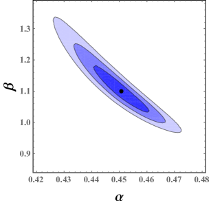
(a) Contour plot for OHD

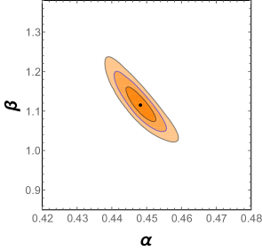
(b) Contour plot for combined OHD+BAO

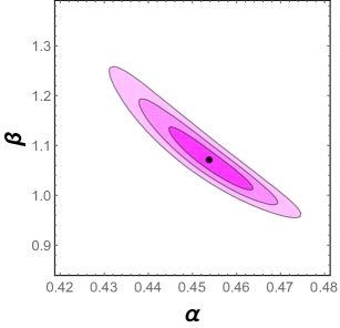
(c) Contour plot for combined OHD+SN

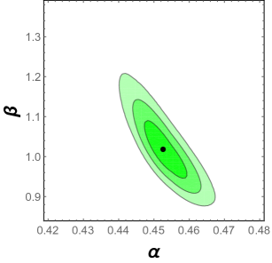
(d) Contour plot for combined SN+BAO

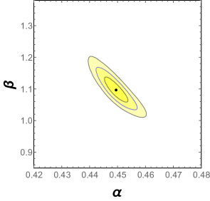
(e) Contour plot for combined OHD+SN+BAO

Figure 1: Figures show the contour plots for likelihood values of the model parameters $\alpha$ & $\beta$ with samples of OHD, SN, BAO and some combined datasets at 1-$\sigma$, 2-$\sigma$, 3-$\sigma$ levels.

We tabulate the constrained values of the model parameters $\alpha$ & $\beta$ as follows together with the minimum chi square values. Also, we calculate the values of deceleration parameter for different datasets at present ($z=0$) which are obtained from Fig. 1.

Table.2: Constrained values of the model parameters with minimum chi square values and the present values of deceleration parameter

$Datasets$	$\alpha$	$\beta$	$\chi_{\min}^{2}/dof$	$q(z=0)$	$z_{t}$
$H(z)$	$0.45_{-0.02}^{+0.02}$	$1.10_{-0.11}^{+0.11}$	$0.574$	$-0.50_{-0.11}^{+0.11}$	$-0.76_{-0.37}^{+0.27}$
$H(z)+BAO$	$0.44_{-0.02}^{+0.02}$	$1.11_{-0.11}^{+0.11}$	$0.564$	$-0.48_{-0.11}^{+0.13}$	$-0.73_{-0.11}^{+0.13}$
$H(z)+SN$	$0.45_{-0.02}^{+0.02}$	$1.07_{-0.11}^{+0.11}$	$0.940$	$-0.51_{-0.15}^{+0.23}$	$-0.74_{-0.15}^{+0.23}$
$SN+BAO$	$0.45_{-0.01}^{+0.02}$	$1.01_{-0.11}^{+0.11}$	$0.966$	$-0.57_{-0.16}^{+0.21}$	$-0.85_{-0.60}^{+0.44}$
$H(z)+SN+BAO$	$0.44_{-0.01}^{+0.01}$	$1.09_{-0.11}^{+0.11}$	$0.936$	$-0.50_{-0.11}^{+0.12}$	$-0.67_{-0.36}^{+0.26}$

The error bar plots of the $OHD$ sample and the Union $2.1$ compilation sample are shown in the Fig. 2.

$\begin{array}[]{c@{\hspace{.1in}}c}\includegraphics[width=216.81pt,height=180.67499pt]{6.pdf}\hfil\hskip 7.22743pt&\includegraphics[width=216.81pt,height=180.67499pt]{7.pdf}\\ \mbox{(}a)\hfil\hskip 7.22743pt&\mbox{(}b)\end{array}$

Figure 2: Figures (a) and (b) are respectively the error bar plots for $57$ data points from OHD and for $580$ points from Union$2.1$ compilation supernovae datasets. Solid red lines are presented model compared with $\Lambda$CDM model shown in black dashed lines in both the plots.

IV Evolution of cosmological and cosmographic parameters

The very useful way of describing an increasing or decreasing rate of expansion of the universe is to study the deceleration parameter. The form of deceleration parameter considered here (see equation (16)) contain two parameters which are constrained through some datasets, so we can now discuss it’s evolution with the numerical values. The following plot shows the evolution of $q$ w.r.t. redshift $z$ that explains it’s evolution in the near past, present evolution and the signature flipping behavior for the above constrained values of the model parameters $\alpha$ and $\beta$ (see Fig. 3). As we know, although the negative value of q corresponds to the accelerated period, the positive q refers to the decelerating phase. We can see from the figure 3 that the deceleration parameter q varies with z from positive to negative. This demonstrates a transition from early deceleration to the universe’s present acceleration.

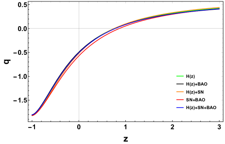
Figure 3: Evolution of the deceleration parameter as a function of redshift for different constrained values of model parameters $\alpha$ & $\beta$ showing phase transition and present acceleration.

If we talk about equation of state parameter (EoS), then we see that it reflects the relation of energy density and pressure which basically connects to the evolution of the universe. The EoS parameter for radiation dominated phase is illustrated by $\omega=\frac{1}{3}$ followed by the dust phase i.e matter dominated phase with $\omega=0$. The cosmological constant is represented by $\omega=-1$ which is also known as $\Lambda$CDM model. Also $-1<\omega<0$, shows the quintessence phase whereas $\omega<-1$ is the phantom stage.

Now, using equations (15) and (16) in equations (9), (10) and (11), we have the expressions for the pressure, the energy densities and the potential function of the scalar field can be written as,

$$p_{eff}=-H_{0}^{2}\left(2\frac{(\beta(z+1))^{8\alpha^{2}}+\alpha^{2}\left(4-8(\beta(z+1))^{8\alpha^{2}}\right)+1}{(\beta(z+1))^{8\alpha^{2}}+1}+1\right)\frac{\left((\beta(z+1))^{8\alpha^{2}}+1\right)^{3}}{\left(\beta^{8\alpha^{2}}+1\right)^{3}(z+1)^{8\alpha^{2}}}\text{.}$$ (20)

$$\rho_{eff}=3H_{0}^{2}\frac{\left((\beta(z+1))^{8\alpha^{2}}+1\right)^{3}}{\left(\beta^{8\alpha^{2}}+1\right)^{3}(z+1)^{8\alpha^{2}}}\text{.}$$ (21)

$$\rho_{\phi}=3H_{0}^{2}\frac{\left((\beta(z+1))^{8\alpha^{2}}+1\right)^{3}}{\left(\beta^{8\alpha^{2}}+1\right)^{3}(z+1)^{8\alpha^{2}}}-3H_{0}^{2}\Omega_{m_{0}}(1+z)^{3}\text{. }$$ (22)

where $\Omega_{m_{0}}=\frac{\rho_{0}}{3H_{0}^{2}}$. The expression for the potential function $V(\phi)$ of the scalar field is obtained as,

$$V(\phi)=H_{0}^{2}\left(2+\frac{(\beta(z+1))^{8\alpha^{2}}+\alpha^{2}\left(4-8(\beta(z+1))^{8\alpha^{2}}\right)+1}{(\beta(z+1))^{8\alpha^{2}}+1}\right)\frac{\left((\beta(z+1))^{8\alpha^{2}}+1\right)^{3}}{\left(\beta^{8\alpha^{2}}+1\right)^{3}(z+1)^{8\alpha^{2}}}-1.5H_{0}^{2}\Omega_{m_{0}}(1+z)^{3}\text{.}$$ (23)

The evolution of the effective energy density of the matter energy density, scalar field energy density and the scalar field potential are shown in the figure.

$\begin{array}[]{c@{\hspace{.1in}}c}\includegraphics[width=216.81pt,height=180.67499pt]{8.pdf}\hfil\hskip 7.22743pt&\includegraphics[width=216.81pt,height=180.67499pt]{9.pdf}\\ \mbox{(}a)\hfil\hskip 7.22743pt&\mbox{(}b)\end{array}$

Figure 4: In this figure panel (a) shows the evolution of effective energy density, matter energy density and scalar field energy density as a function of redshift while panel (b) shows the evolution of scalar field potential $V(\phi)$ as function of redshift.

$\begin{array}[]{c@{\hspace{.1in}}c}\includegraphics[width=216.81pt,height=180.67499pt]{Omega.pdf}\hfil\hskip 7.22743pt&\end{array}$

Figure 5: The figure shows the evolution of the density parameters for matter ($\Omega_{m}$) and the scalar field ($\Omega_{\phi}$) as functions of redshift $z$.

Now, the effective equation of state parameter $\omega_{eff}=\frac{p_{eff}}{\rho_{eff}}$ reads as,

$$\omega_{eff}=-\frac{1}{3}\left(2\frac{(\beta(z+1))^{8\alpha^{2}}+\alpha^{2}\left(4-8(\beta(z+1))^{8\alpha^{2}}\right)+1}{(\beta(z+1))^{8\alpha^{2}}+1}+1\right).$$ (24)

Moreover, with the dark energy domination, the expression for the equation of state of scalar field or the dark energy $\omega_{\phi}$ can be written as,

$$\omega_{\phi}=\frac{1}{3}\frac{\frac{\left((\beta(1+z))^{8\alpha^{2}}+1\right)^{3}}{\left(\beta^{8\alpha^{2}}+1\right)^{3}(1+z)^{8\alpha^{2}}}\left(2\frac{(\beta(z+1))^{8\alpha^{2}}+\alpha^{2}\left(4-8(\beta(z+1))^{8\alpha^{2}}\right)+1}{(\beta(z+1))^{8\alpha^{2}}+1}+1\right)}{\Omega_{m0}(1+z)^{3}-\frac{\left((\beta(1+z))^{8\alpha^{2}}+1\right)^{3}}{\left(\beta^{8\alpha^{2}}+1\right)^{3}(1+z)^{8\alpha^{2}}}}.$$ (25)

$\begin{array}[]{c@{\hspace{.1in}}c}\includegraphics[width=216.81pt,height=180.67499pt]{10.pdf}\hfil\hskip 7.22743pt&\includegraphics[width=216.81pt,height=180.67499pt]{11.pdf}\\ \mbox{(}a)\hfil\hskip 7.22743pt&\mbox{(}b)\end{array}$

Figure 6: In this figure, the panel (a) shows the evolution of effective EoS parameter ($\omega^{eff}$) for the constrained values of $\alpha=0.449451$ and $\beta=1.096408$ and the panel (b) shows the evolution of scalar field (or dark energy) EoS parameter ($\omega_{\phi}$) as functions of redshift.

In Fig 4, the energy density $\rho_{eff}$, $\rho_{m}$ and $\rho_{\phi}$ is showing positive behavior for according to different value of $\Omega_{m_{0}}$. It is seen that the energy density is higher for the effective energy density of the matter field if compared with energy density in the presence of scalar field. Also the evolution of scalar field potential is shown which is responsible for negative pressure.

The evolution density parameter for matter and scalar field is shown in Fig5 for different values of $\Omega_{m_{0}}$. Also, in Figs 6, the behavior of $\omega_{eff}$ and $\omega_{\phi}$ are shown for the constrained values of $\alpha=0.449451$ and $\beta=1.096408$ and some chosen values values of the matter density parameter $\Omega_{m_{0}}$ as shown in the figure. This analysis also put constrain on the $\Omega_{m_{0}}$ value which should be $\leq 0.269$ for smooth evolution of the scalar field (or dark energy) EoS parameter. The curve shows a negative behavior at early times and evolve through different phases of acceleration, deceleration and finally to phantom phase. It can also be seen that for some values of $\Omega_{m_{0}}$, the curves shows a singularity. The transition from one phase to the other indicates the possibility for evolution of the universe. Planck observations are known to be considered the best approximations of cosmological effects. Planck’s 2018 findings indicate that the Hubble constant is $H_{0}=67.8\pm 0.9$ km $s^{-1}Mpc^{-1}$ and $\Omega_{m}=0.308\pm 0.012$, but the obtained value of $\Omega_{m_{0}}$ is 0.269. This deviation point towards a tension with Planck results.

Moreover, the higher order derivatives of deceleration parameter $q$ such as jerk ($j$), snap ($s$) and lerk ($l$) are important in understanding the past and future evolution of the universe sanjay . They are represented as Pan :

$$j(z)=(1+z)\frac{dq}{dz}+q(1+2q),$$ (26)

$$s(z)=-(1+z)\frac{dj}{dz}-j(2+3q),$$ (27)

$$l(z)=-(1+z)\frac{ds}{dz}-s(3+4q).$$ (28)

These higher order derivatives can be useful in understanding the future evolution of the universe owing to the fact that $q(z)$ can be strictly constrained from observations. The jerk parameter $j$ is related to the third time derivative of $a$ as a higher-order derivative of the scale component. The higher-order derivatives can describe the dynamics of the universe and may be connected to the appearance of abrupt future singularities Pan ; Dabrowski . In the statefinder diagnostic, the jerk parameter $j$ is often used to discriminate against various dark energy or modified gravity models. Zhai Zhai proposed different kinds of parameterizations of $j$ as a function of the redshift z. A vital feature of $j$ is that for the $\Lambda$CDM model, $j=1$ always. The deviation from $j=1$ enables us to constrain the departure from the $\Lambda$CDM value.. The value of $j_{0}$ according to constrain value of $\alpha$ and $\beta$ is $j_{0}=-0.98_{-0.02}^{+0.06}$ Mamon . The behavior of $j(z)$ is shown in Figs. 7. It can be clearly observed that $j(z)$ increases with redshift indicating a decelerated phase in the past and an accelerated phase in future. Interestingly the kinematic quantity $j(z)$ is positive which is a reminiscent of an accelerated expansion. Also note that $j(z)\neq 1$ at $z=0$ which does not correspond to $\Lambda$CDM cosmology. As mentioned in sanjay , this can be thought as an expansion caused purely due to modifications of gravity.

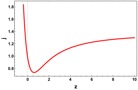
Figure 7: The plots of jerk $j$, snap $s$ and lerk $l$ parameters  vs. redshift $z$ for the constrained values of $\alpha=0.449451$ and $\beta=1.096408$.

V Statefinder diagnostics

The statefinder pairs $\{r,s\}$ and $\{r,q\}$ are the geometrical quantities formulated directly from the metric and are employed to identify various dark energy model. In the literature, the $\{r,s\}$ and $\{r,q\}$ pairs are defined as Statefinder1 .

$$q=-\frac{\ddot{a}}{aH^{2}}\text{, \ \ }r=\frac{\dddot{a}}{aH^{3}}\text{, \ \ }s=\frac{r-1}{3(q-\frac{1}{2})}\text{.}$$ (29)

The statefinder diagnostic is an useful tool in modern day cosmology and being used to serve the purpose of distinguishing different dark energy models Statefinder2 . In this setup, different trajectories in $r-s$ and $r-q$ planes define the temporal evolution for various dark energy models. In a spatially flat FLRW background, the statefinder pair are respectively $\{r,s\}=\{1,0\}$ and $\{1,1\}$ for $\Lambda$CDM and standard cold dark matter (SCDM). In the $r-s$ and $r-q$ planes, the departure of any dark energy model from these fixed points are analyzed. The pairs $\{r,s\}$ and $\{r,q\}$ for our model are shown in figure below.

$\begin{array}[]{c@{\hspace{.1in}}c}\includegraphics[width=216.81pt,height=180.67499pt]{r-s.pdf}\hfil\hskip 7.22743pt&\includegraphics[width=216.81pt,height=180.67499pt]{r-q.pdf}\\ \mbox{(}a)\hfil\hskip 7.22743pt&\mbox{(}b)\end{array}$

Figure 8: Figures (a) and (b) shows the behavior of r-s and r-q plane in red color respectively for the constrained values of $\alpha=0.449451$ and $\beta=1.096408$.

In Fig. 8(a) we show the temporal evolution of the dark energy model mimicked by our model. It is observed that at early times, the model presumes values in the range $r>1$ and $s<0$ and therefore represents a Chaplygin gas type dark energy model. Nonetheless, the model evolves into a Quintessence type dark energy model at some point but then quickly reverts back into CG gas at late times. Interestingly, it can be clearly observed that throughout its temporal evolution, the model deviates significantly from the point $\{r,s\}=\{1,0\}$. In Fig. 8(b) we show the temporal evolution of our model in the $\{r,q\}$ to get additional information regarding the parametrization. In this diagnostic plane, the solid line in the middle depicts the evolution of the standard $\Lambda$CDM cosmological model and also divides the plane into two equal halves with the lower half belonging to Quintessence dark energy models and the upper half to Chaplygin gas dark energy models. We clearly see that the profile starts from the region $q>0$ and $r>1$ which corresponds to the SCDM universe. This is then followed by the region $r<1$ and $q<0$ and finally approaches to towards the de-Sitter phase with $r=1,q=-1$.

VI Conclusion

In this paper we have considered the scalar field with positive potential to study the accelerated expansion of the universe. To explain the late-time acceleration, the EoS parameter $\omega$ must be negative as this implies the cosmological pressure is negative. Negative cosmological pressure is the hallmark of the presence of dark energy as this is only cosmic entity which posses an anti-gravity effect. The potential $V(\phi)$ is responsible for negative pressure.

In order to solve the field equations, we took the assistance of a supplementary equation since the value of $\rho_{\phi}$ and $p_{\phi}$ is difficult to obtain. In this work, we employ a second degree parametrization of deceleration parameter first proposed in Bakry and Shafeek . We used the latest 57 points of $H(z)$ dataset in the redshift range $0.07\leq z\leq 2.42$, 580 points of SN data and BAO datasets to constrained the model parameters using $\chi^{2}$ minimization technique. The values of the parameters $\alpha\ \&\ \beta$ considered here from all the datasets given in Table 2, the present model shows a smooth transition for the deceleration parameter (see Fig. 3) from the deceleration ($q>0$) phase to the present acceleration ($q<0$) phase of the Universe. It has been found that the values of transition redshift $z_{t}$ (from decelerated phase to accelerated expansion) and the values of present deceleration parameter $q_{0}$ depends on the model parameters $\alpha\ \&\ \beta$. It is interesting to note that the values of $z_{t}=0.67_{-0.36}^{+0.26}$ and $q_{0}=-0.50_{-0.11}^{+0.12}$ obtained in our model are in good agreement with the recent results as reported in Jesus/2020 and the references therein. Further, we have studied the other kinematical parameter like jerk parameter using the combined datasets ($H(z)+SN+BAO$). An alternative to describing cosmological models similar to the $\Lambda$CDM model of concordance is the jerk parameter. For LCDM model , the value of j is 1. The deviation from $j=1$ enables us to constrain the departure from the $\Lambda$CDM value. According to the restricted value of $\alpha$ and $\beta$, the value of $j_{0}=-0.98_{-0.02}^{+0.06}$ (close to 1). The jerk parameter increasing with respect to redshift indicating the accelerated phase in the future Universe.
Also, the evolution of $\omega_{eff}$ and $\omega_{\phi}$ is shown for the constrained $\alpha=0.449451$ and $\beta=1.096408$ values and some of the chosen $\Omega_{m_{0}}$ parameter density values. The transition from positive to negative values indicates the decelerated to accelerated phase of the universe. This study also constrains the value of $\Omega_{m_{0}}$ which should be $\leq 0.269$ for the smooth evolution of the EoS parameter scalar field. It can also be shown that the curves display a singularity for specific values of $\Omega_{m_{0}}$. It is understood that Planck observations are regarded as the best approximations of cosmological results. Planck’s 2018 results suggest that $H_{0}=67.8\pm 0.9$ km $s^{-1}Mpc^{-1}$ and $\Omega_{m}=0.308\pm 0.012$ are the Hubble constants, but the obtained value of $\Omega_{m_{0}}$ is 0.269 which results in tension with Planck approximations.

Furthermore, to understand the parametrization from a cosmological point of view, we also diagnose it geometrically using $\{r,s\}$, $\{r,q\}$ planes and $Om(z)$ parameter. We observe that at early times, the model represents a Chaplygin gas type dark energy model and later evolves into a Quintessence type dark energy model at some point but then quickly reverts back into CG gas at late times. Interestingly, the model deviates significantly from the point $\{r,s\}=\{1,0\}$ and therefore do not coincide with $\Lambda$CDM cosmology throughout the cosmic aeon.

- (1) A. G. Riess et al., Astron. J. 116, 1009 (1998).
- (2) S. Perlmutter et al., Astrphys. J. 517, 565 (1999).
- (3) Supernova Cosmology Project collaboration, Astrophys. J. 686, 749 (2008); R. Amanullah et al., Astrophys. J. 716, 712 (2010); Supernova Cosmology Project collaboration, Astrophys. J. 746, 85 (2012).
- (4) WMAP collaboration, Astrophys. J. Suppl. 192, 18 (2011); D. Larson et al., Astrophys. J. Suppl. 192, 16 (2011) ; Planck collaboration, Planck 2013 results. Astron. Astrophys. 571, A16 (2014) .
- (5) SDSS collaboration, Astrophys. J. 633, 560 (2005); SDSS collaboration, Astron. J. 142, 72 (2011); BOSS collaboration, Astron. J. 145, 10 (2013).
- (6) O. Farooq, B. Ratra, Astrophys. J. 766, L7 (2013); O. Farooq et al. Astrophys. J. 835, 26 (2017).
- (7) B. Ratra, P. J. E Peebles, Phys. Rev. D 37, 3406 (1988); R. R. Caldwell et al., Phys. Rev. Lett. 80, 1582 1988; C. Armendariz-Picon et al., Phys. Rev. D 63, 103510 (2001); T. Buchert, Gen. Relativ. Gravit. 32, 105 (2000); P. Hunt, S. Sarkar, Mon. Not. R. Astron. Soc. 401, 547 (2010); K. Tomita, Mon. Not. R. Astron. Soc. 326, 287 (2001); B. Pandey, Mon. Not. R. Astron. Soc. 485, L73 (2019); B. Pandey, Mon. Not. R. Astron. Soc. 471, L77 (2017); K. A. Milton, Gravit. Cosmol. 9, 66 (2003); D. Easson et al., Phys. Lett. B 696, 273 (2011); D. Pavón , N. Radicella, Gen. Relativ. Gravit. 45, 63 (2013); N. Radicella, D. Pavón, Gen. Relativ. Gravit. 44, 685 (2012).
- (8) V. Sahni, The Physics of the Early Universe. Lecture Notes in Physics, Springer, Berlin, Heidelberg 653, 141-179 (2004): V. Sahni, and A. Starobinsky, Int. J. Mod. Phys. D 9, 373 (2000): Luis P. Chimento et al., Int. J. Mod. Phys. D 5, 1, 71-84 (1996).
- (9) A.Y. Kamenshchik et al., Phys. Lett. B 511, 265 (2001).
- (10) R. R. Caldwell, M. Kamionkowski, N. N. Weinberg, Phys. Rev. Lett. 91, 071301 (2003); K. Bamba et al. Astrophys Space Sci 342, 155 (2012).
- (11) G. S. Sharov, V. O. Vasiliev, Mathematical Modelling and Geometry, 6, 1 (2018).
- (12) E. Di Valentino, A. Melchiorri, J. Silk, arXiv: 2003.04935.
- (13) J.K.Singh , R. Nagpal, Eur. Phys. J.C. 80:295 (2020).
- (14) N. Aghanim et al. Planck Collaboration arXiv: 1807.06209.
- (15) A.G. Riess, S. Casertano et al. Astrophys. J. 876, no.1 85 (2019).
- (16) D.M. Scolnic et al. ApJ 859, 101 2018.
- (17) A. A. Starobinsky, J. Exp. Theor. Phys. Lett. 68, 757 (1998).
- (18) D. Huterer, M. S. Turner, Phys. Rev. D 60, 081301 (1999).
- (19) T. D. Saini et al. Phys. Rev. Lett. 85, 1162 (2000).
- (20) Z. K. Guo, N. Ohta, Y. Z. Zhang, Phys. Rev. D 72, 023504 (2005).
- (21) A. Mukherjee, Mon. Not. R. Astron. Soc. 460, 273 (2016).
- (22) R. Nair, S. Jhingan, D. Jain, J. Cosmol. Astropart. Phys. 01, 005 (2014).
- (23) A. A. Mamon, K. Bamba, Eur. Phys. J. C 78, 862 (2018).
- (24) C. Shapiro, M. Turner, Astrophys. J. 649, 563 (2006); D. Rapetti, S. W. Allen, M. A. Amin, R. D. Blandford, Mon. Not. R. Astron. Soc. 375, 1510 (2007); A. Aviles, C. Gruber, O. Luongo, H. Quevedo, Phys. Rev. D 86, 123516 (2012); S. D. P. Vitenti, M.Penna-Lima, J. Cosmol. Astropart. Phys. 09, 045 (2015); S. Capozziello, R. D�, Agostino, O. Luongo, Mon. Not. R. Astron. Soc. 476, 3 (2018).
- (25) J. Lu, L. Xu, M. Liu, Phys. Lett. B 699, 246(2011); L. Xu, Y. Wang, Phys. Lett. B 702, 114(2011); I. Sendra, R. Lazkoz, Mon. Not. R. Astron. Soc. 422, 776 (2012); S. del Campo, I. Duran, R. Herrera, D. Pavon, Phys. Rev. D 86, 083509 (2012); A. R. Neben, M. S. Turner, Astrophys. J. 769, 133 (2013); A. Mukherjee, N. Banerjee, Class. Quant. Grav. 34, 035016(2017); L. Tedesco, Eur. Phys. J. Plus 133, 188(2018).
- (26) S. Das et al., Res. Astron. Astrophys. 18, 131 (2018).
- (27) N. Banerjee et al., Gen. Relativ. Gravit. 37(10): 1695-1703 (2005).
- (28) Planck 2018 results. VI. Cosmological parameters [arXiv:1807.06209].
- (29) S. K. J. Pacif et al., Int. J. Geom. Meth. Mod. Phys., 14(7), 1750111 (2017).
- (30) M.A. Bakry, Aryn T. Shafeek, Astrophys Space Sci. 364, 135 (2019).
- (31) R. Giostri, M. V. d. Santos, I. Waga, R. R. R. Reis, M. O. Calvao and B. L. Lago, J. Cosm. Astrop. Phys. 1203, 027 (2012).
- (32) P. A. R. Ade et al. [Planck Collaboration], Astron. Astrophys., 571, A16 (2014).
- (33) N. Suzuki et al., Astrophys. J., 746, 85 (2012).
- (34) N. Padmanabhan, X. Xu, D. J. Eisenstein, R. Scalzo, A. J. Cuesta, K. T. Mehta et al., Mon. Not. Roy. Astron. Soc. 427, 2132 (2012).
- (35) F. Beutler, C. Blake, M. Colless, D. H. Jones, L. Staveley-Smith, L. Campbell et al., Mon. Not. Roy. Astron. Soc. 416, 3017 (2011).
- (36) BOSS collaboration, L. Anderson et al., Mon. Not. Roy. Astron. Soc. 441, 24 (2014).
- (37) C. Blake et al., Mon. Not. Roy. Astron. Soc. 425, 405 (2012).
- (38) G. Hinshaw et al., Astrophys. J. Suppl., 208, 19 (2013).
- (39) S. Mandal, S. Bhattacharjee, S.K.J. Pacif, P.K. Sahoo., Physics of the Dark Universe 28, 100551 (2020), https://doi.org/10.1016/j.dark.2020.100551.
- (40) S. Pan, A. Mukherjee, N. Banerjee, Mon. Not. R. Astron. Soc. 477, 1189 (2018).
- (41) M.P. Dabrowski, Phys. Lett. B 625, 184 (2005).
- (42) Ahong-Xu-Zhai et al., Phys. Lett. B 727, 8-20 (2013).
- (43) A. AI Mamon, K. Bamba, Eur. Phys. J. C 78, 862 (2018).
- (44) V. Sahni, T. D. Saini, A. A. Starobinsky and U. Alam, JETP Lett. 77, 201 (2003); U. Alam, V. Sahni, T. D. Saini, A. A. Starobinsky, Mon. Not. R. Astron. Soc. 344, 1057 (2003).
- (45) M. Sami et al., Phys. Rev. D 86, 103532 (2012); R. Myrzakulov, M. Shahalam, J. Cosm. Astrop. Phys. 1310, 047 (2013); S. Rani et al., J. Cosm. Astrop. Phys. 1503, 031 (2015).
- (46) J. F. Jesus et al. J. Cosm. Astrop. Phys. 04, 053 (2020).