Deep Two-Stage High-Resolution Image Inpainting

Abstract

In recent years, the field of image inpainting has developed rapidly, learning based approaches show impressive results in the task of filling missing parts in an image. But most deep methods are strongly tied to the resolution of the images on which they were trained. A slight resolution increase leads to serious artifacts and unsatisfactory filling quality. These methods are therefore unsuitable for interactive image processing. In this article, we propose a method that solves the problem of inpainting arbitrary-size images. We also describe a way to better restore texture fragments in the filled area. For this, we propose to use information from neighboring pixels by shifting the original image in four directions. Moreover, this approach can work with existing inpainting models, making them almost resolution independent without the need for retraining. We also created a GIMP plugin that implements our technique. The plugin, code, and model weights are available at https://github.com/a-mos/High˙Resolution˙Image˙Inpainting.

1 Introduction

Image inpainting is the process of realistically filling unknown or damaged regions of an image. An inpainting algorithm receives as input a corrupted image and a mask; its output is a restored image.

${512\times 512}$
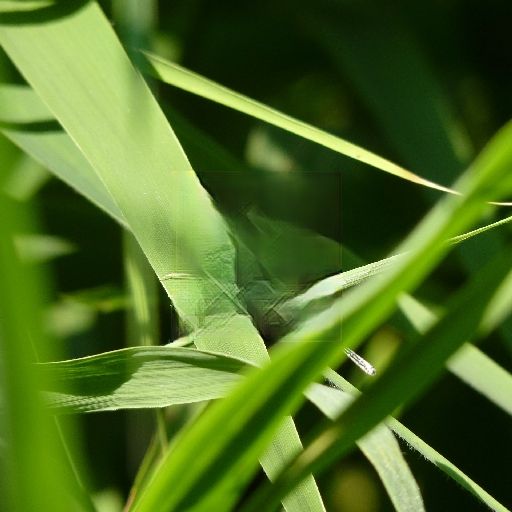
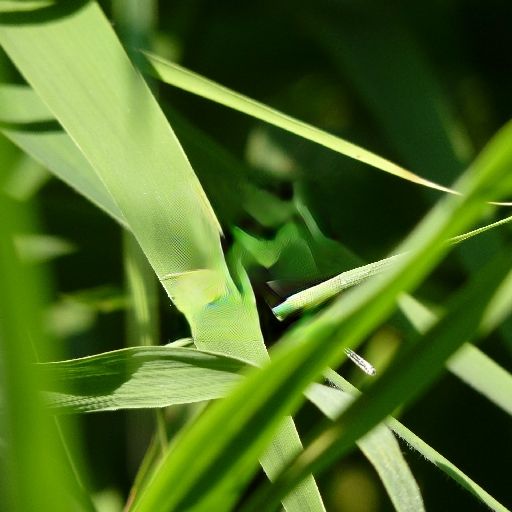
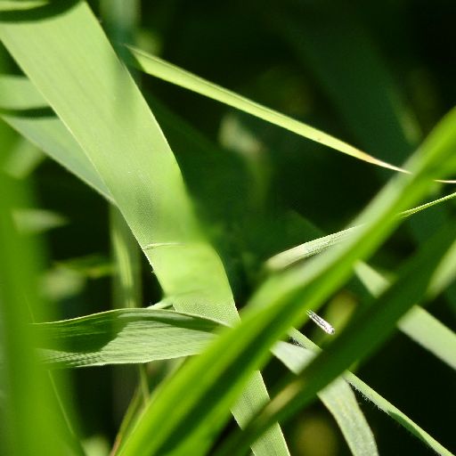
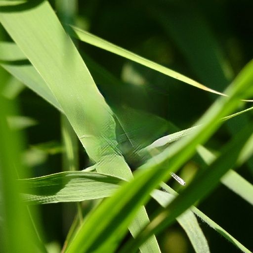
${1024\times 1024}$
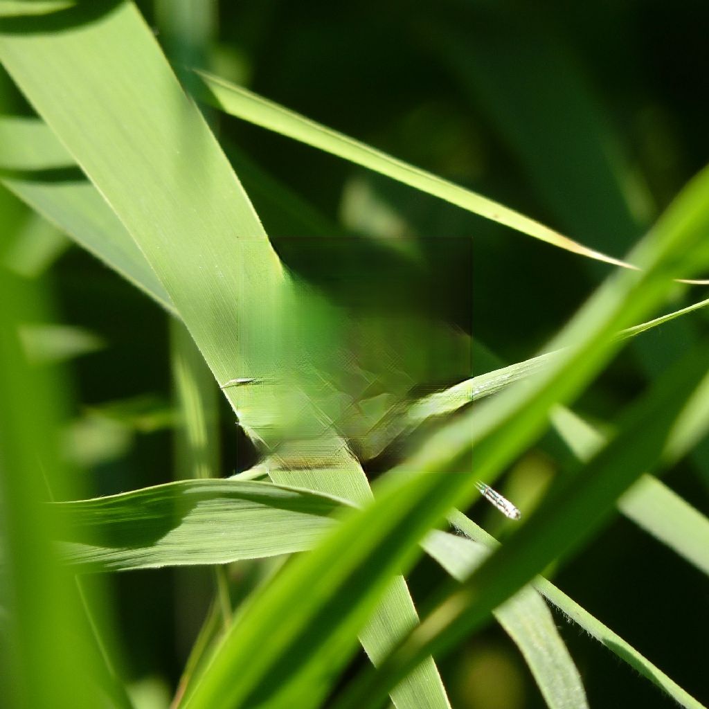
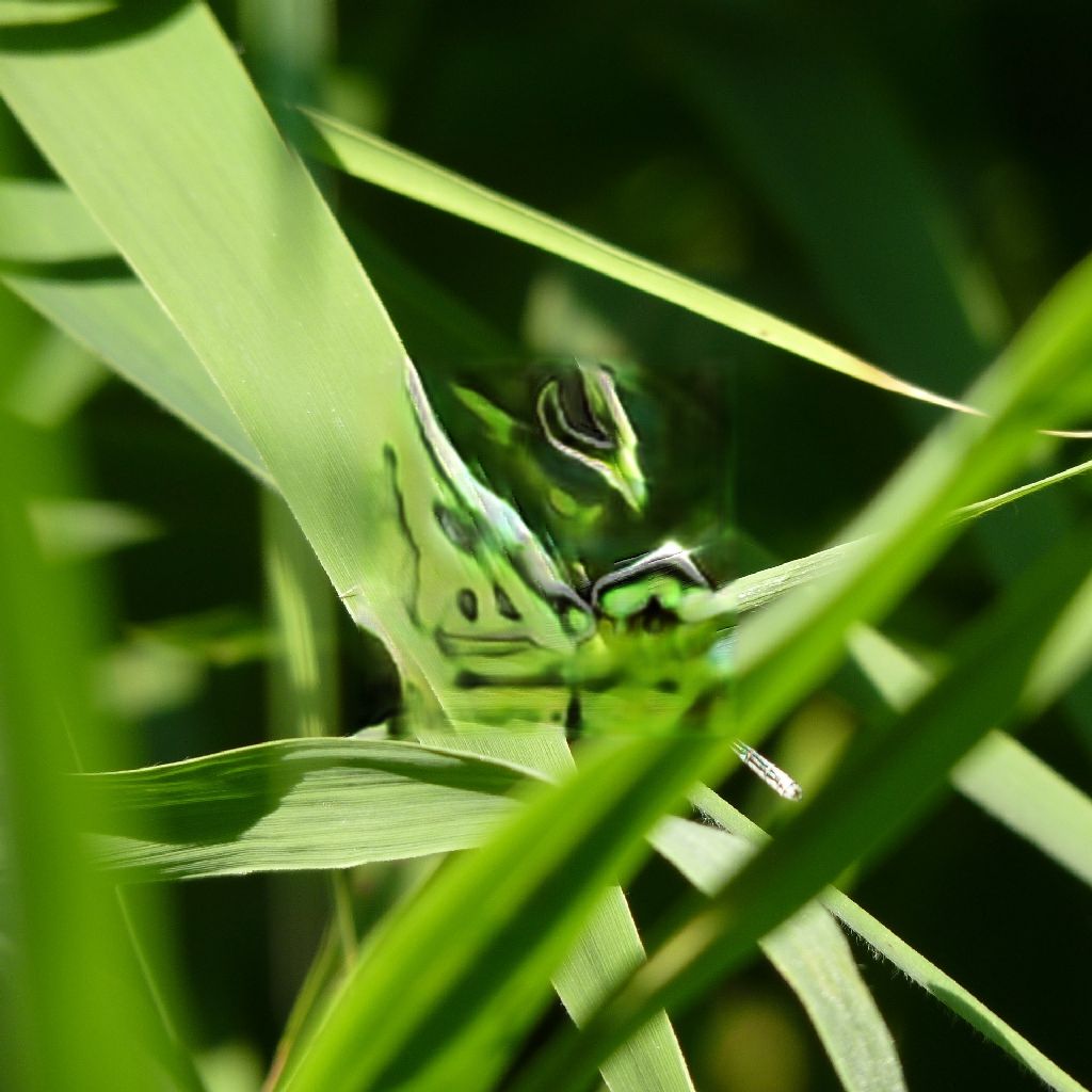
${512\times 512}$
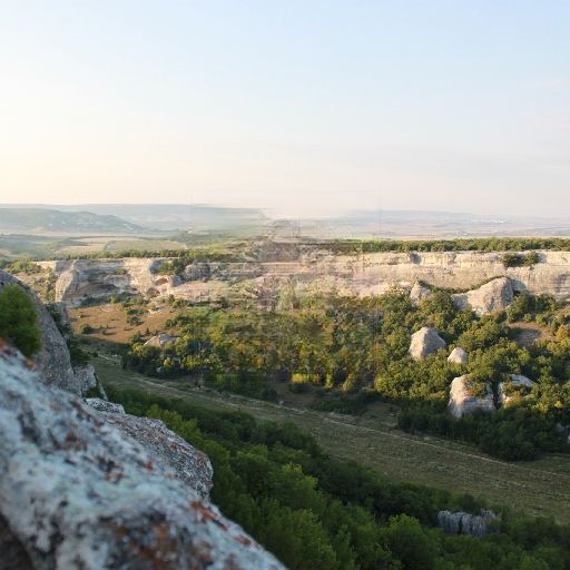
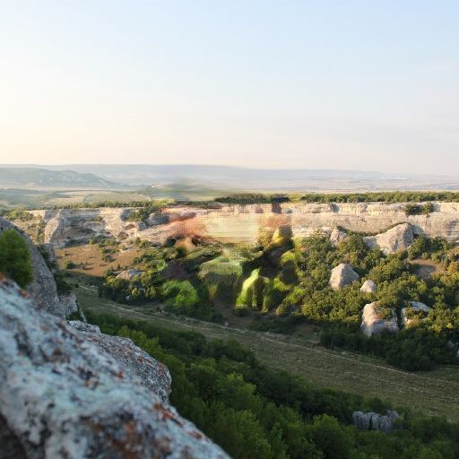
${1024\times 1024}$
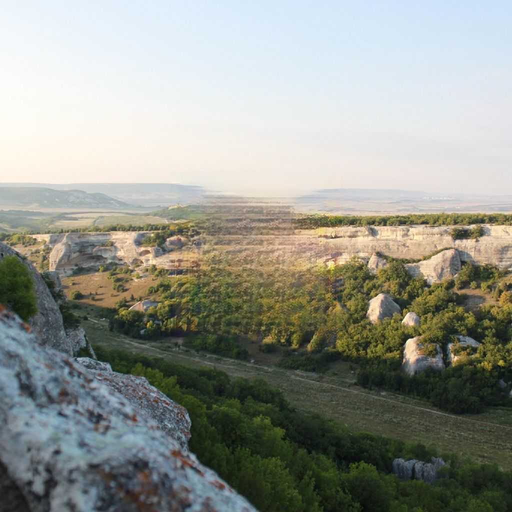
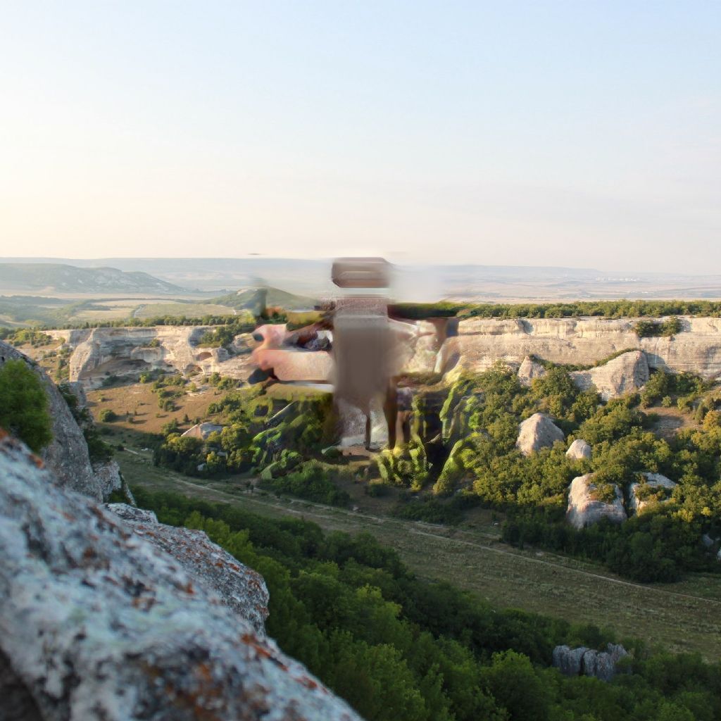
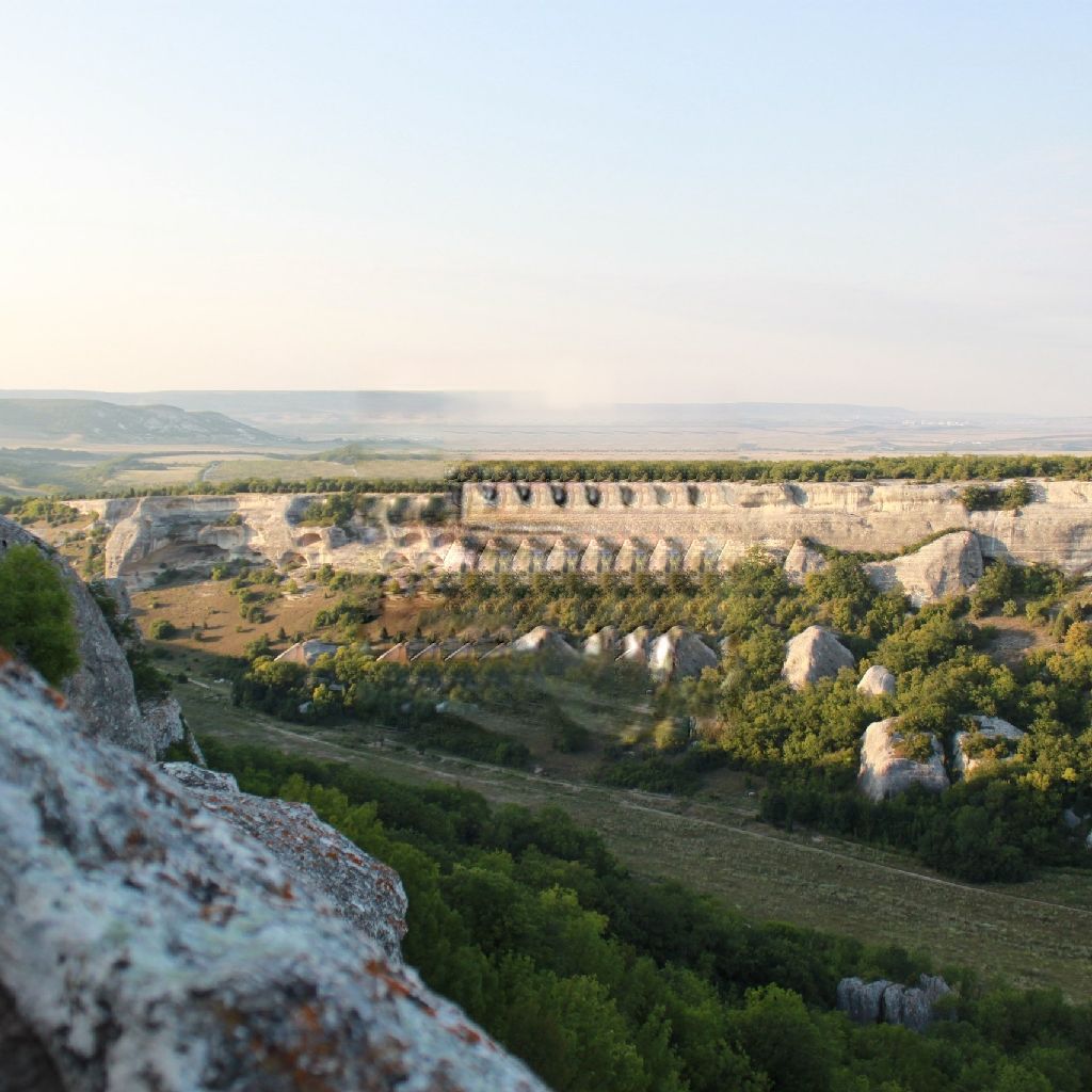
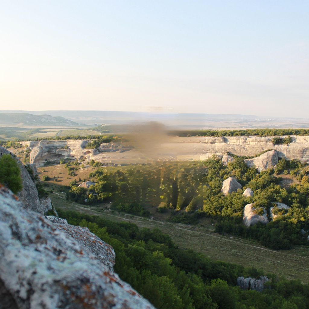
	DFNet	DeepFillv2	HiFill	ProFill	Ours

Figure 1: Methods outputs at different resolutions

In recent years, the progress of neural networks has led to the development of deep inpainting methods. Neural-network methods are strongly tied to the resolution at which they are trained, owing to the lack of receptive field. Most models have an input size less than or equal to 512 pixels. As a result, they are unable to handle images of arbitrary shape — for instance, those in interactive image-processing tools. When the resolution increases, serious artifacts appear in the models. Fig. 1 shows several examples.

In this article, we describe a method that can restore images regardless of resolution. It uses the coarse-to-fine approach, restoring the image structure at low resolution and the texture at high resolution. Also, to improve texture filling, we propose using shifts of the original image that fill the hole and that artificially expand the receptive field by the shift amount. Our approach theoretically works for any inpainting method without retraining.

2 Related Work

The solution to image inpainting problem can take the classical approach of choosing the most suitable patch [1, 2, 3] from the image and sequentially filling the hole. Such methods are good at filling the texture component but poor at filling the structural component. In recent years, the development of neural networks has led to the creation of various deep inpainting methods [4, 5, 6]. Such algorithms avoid using external memory and operate only on the basis of knowledge gained during training. They are better than classical algorithms at restoring an image’s structural features.

Adding to the difficulty of training neural-network methods is that the solution to the inpainting problem is nonunique. Thus, formulating the most suitable loss function for training is difficult. Deep-neural-network features are the best way to evaluate hole-filling quality [7].

Also, the appearance of generative adversarial networks (GANs) [8] formed the basis for creating generative image-filling methods [9, 4, 5, 10, 11, 12], which use adversarial loss as one component of their loss functions.

2.1 Gated Convolutions and Contextual Attention Module

In [10], researchers proposed replacing some of the neural network’s classical convolutions with gated convolutions, an extension of partial convolutions [4]. They also introduced a contextual-attention module, which is a neural-network analog of patch-based algorithms for filling image areas. Their method employs a GAN. Instead of a high-computational-cost contextual-attention module, we propose common shifts as a means of filling texture.

2.2 Deep Fusion Network

The authors of [6] created a fusion block, which allows the network to, at its output, alpha blend each pixel in accordance with the predicted alpha map. They implemented the U-Net [13] architecture in a non-generative-adversarial manner, using the high-level features of VGG16 [14] as loss functions. Our network implements a pretrained DFNet in the first stage, yielding the structural component in low resolution. We avoided a fusion block in our refinement network, since it changes even the unmasked area.

2.3 High-Resolution Inpainting

In [11], researchers proposed modified gated convolutions that decrease the computational complexity, reducing the number of weights. They also suggested splitting the image at high and low frequencies by subtracting the blurry version from the image and using the modified contextual-attention module for aggregation. They trained their refinement network on the small but full images. The goal of our refinement network, on the other hand, is only to restore texture, so we train it on small patches of the original image; when testing, we use the entire image.

3 Proposed Approach

3.1 Data Preparation

For training, we selected all images from DIV2K [15] and some from the Internet. From each image, we cut out three random largest squares. In total, the training sample contained 7,218 images, with an additional 1,650 for validation. We applied to each image a random irregular mask from [4]. Our testing used natural images with a square mask at the center.

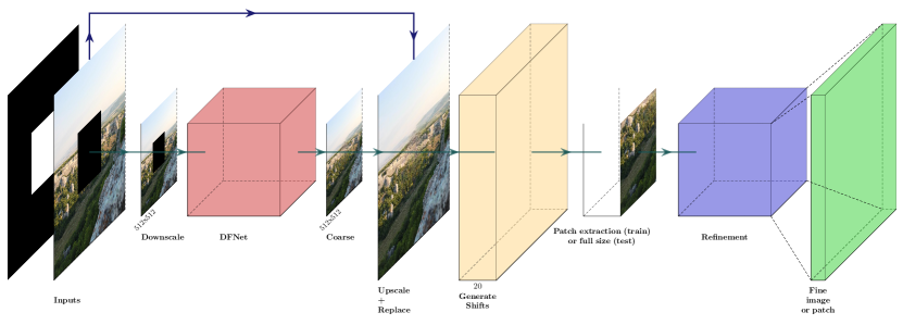
Figure 2: Whole pipeline illustration

Figure 3: Refinement network architecture

3.2 Whole Pipeline

3.2.1 Stage one

The first stage of our algorithm restores the image structure at a low resolution. We initially downscale the image and mask to ${512\times 512}$, then apply the pretrained DFNet [6] to get the coarse result in low resolution. Next we perform an upscale and replace the known region with the corresponding region from the high-resolution image.

Finally we generate shifts of the original image in four directions: left, right, down, up. For our experiments, the shifts were 20% of the image size. Note that during this process, we also recount the masks and mark the pixels in the open areas as invalid. Thus, the first stage yields a 20-channel image: five RGB images (main plus four shifts) and five masks.

3.2.2 Stage two

The second stage restores the texture. To prevent the network from being attached to the structure and to increase training efficiency, we cut out random ${512\times 512}$ patches from the input tensor of depth 20, with the condition that the masked area (from the main mask) is at least 10% but not more than 90% of the patch area. Note that during testing, we skip the patch extraction and simply transmit images in full resolution. The refinement network’s output is a fine filled result. Fig. 3 shows the pipeline.

3.3 Network Architecture

The refinement-network architecture implements the U-Net [13] approach. (An illustration appears in Fig. 3). Note that after each layer — except for the last one — we used Batch Normalization [16]. The figure shows encoder filter sizes; all decoder filters are ${3\times 3}$.

3.4 Loss Function

We trained our network in a non-generative-adversarial manner. Following [6] as a loss function, we used a linear combination:

$$\mathcal{L}=0.1\cdot\mathcal{L}_{\_}{tv}+6.0\cdot\mathcal{L}_{\_}{1}+0.1\cdot\mathcal{L}_{\_}{p}+240.0\cdot\mathcal{L}_{\_}{s}$$ (1)

Where for reference image $\mathbf{I}$ and predicted $\hat{\mathbf{I}}$:

${L}_{\_}{tv}$ — total variation distance in the masked area

${L}_{\_}{1}$ — distance which is calculated as

$$\mathcal{L}_{\_}{1}=\frac{1}{CHW}\left\|\mathbf{I}-\hat{\mathbf{I}}\right\|_{\_}{1}$$ (2)

Where $C,W,H$ are the number of channels, width, and height respectively.

${L}_{\_}{p},{L}_{\_}{s}$ — Perceptual and Style Losses [17]:

$$\mathcal{L}_{\_}{p}=\sum_{\_}{j\in J}\left\|\psi_{\_}{j}\left(\mathbf{I}\right)-\psi_{\_}{j}\left(\hat{\mathbf{I}}\right)\right\|_{\_}{1}$$ (3)

$$\mathcal{L}_{\_}{s}=\sum_{\_}{j\in J}\left\|G_{\_}{j}\left(\mathbf{I}\right)-G_{\_}{j}\left(\hat{\mathbf{I}}\right)\right\|_{\_}{1}$$ (4)

Where $J$ is set of indices in VGG16, $\psi_{\_}{j}$ is $j-th$ feature layer. And $G_{\_}{j}$ is Gram matrix of $j-th$ feature layer.

4 Experiments

Our network training used the Adam [18] optimizer with default settings. It took two days on two Nvidia Tesla P100 GPUs with a batch size of 18 images. Note that we trained only the network from the second stage. For optimization, we calculated the first stage’s output separately.

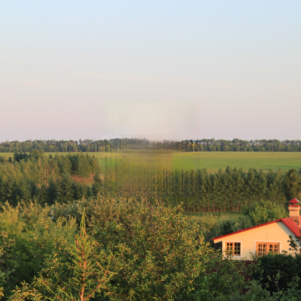
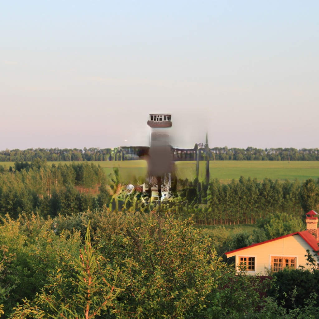
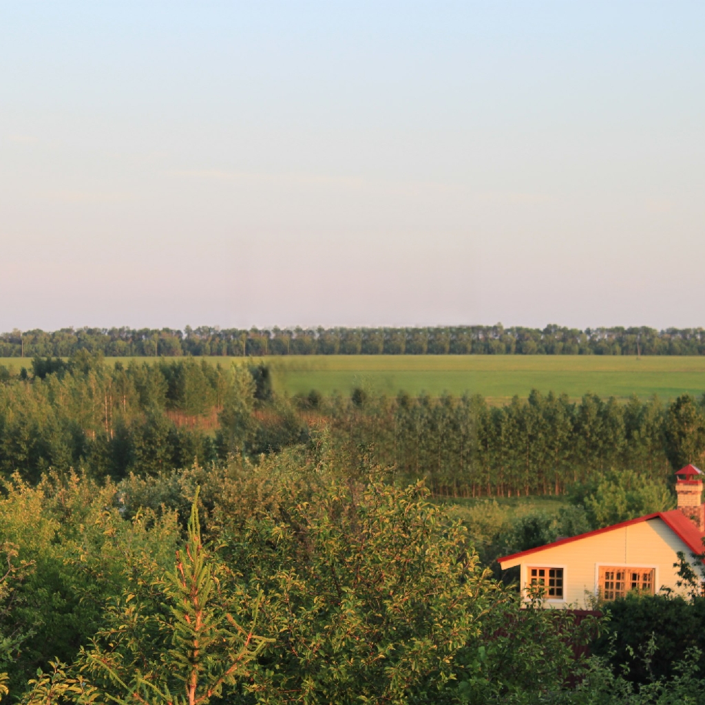
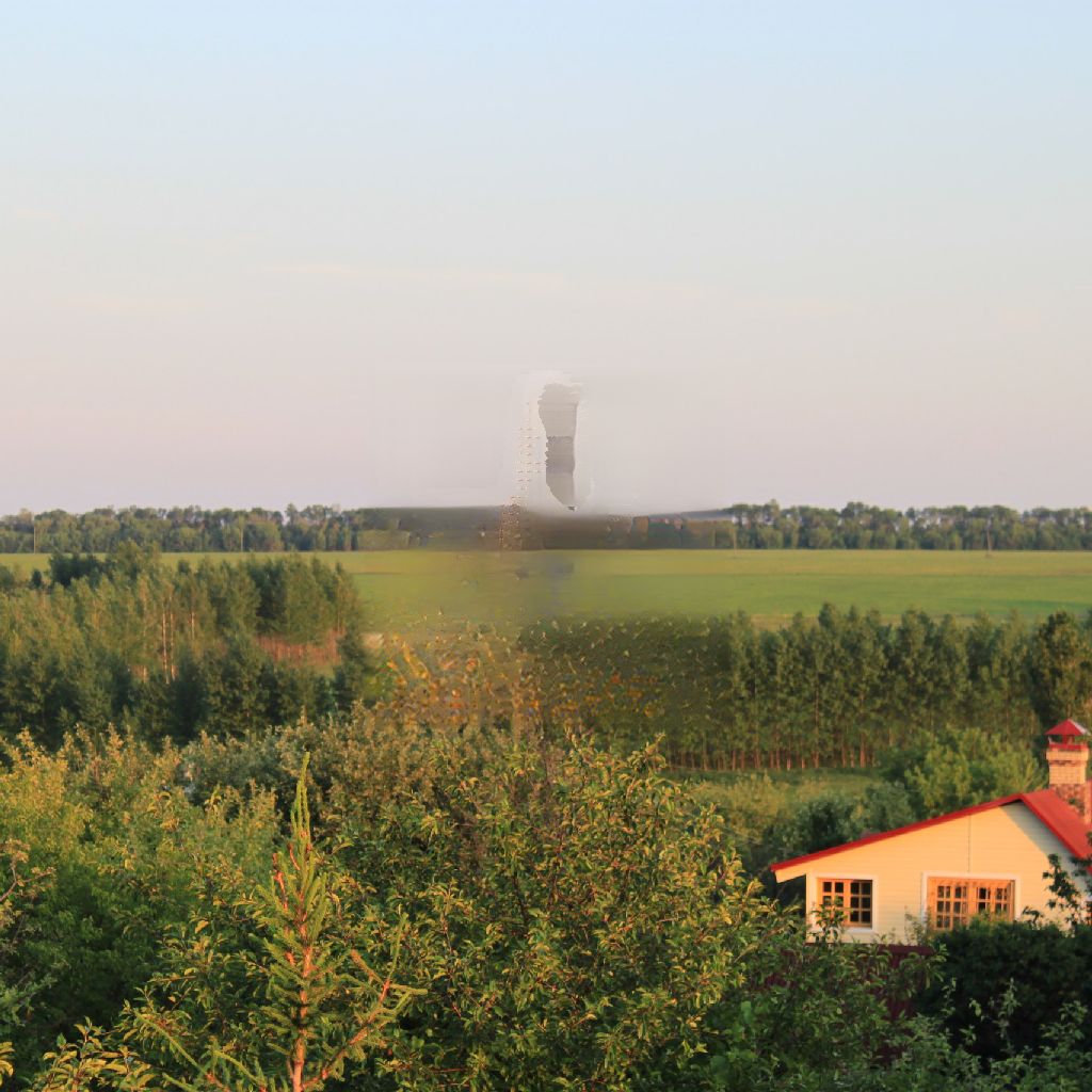
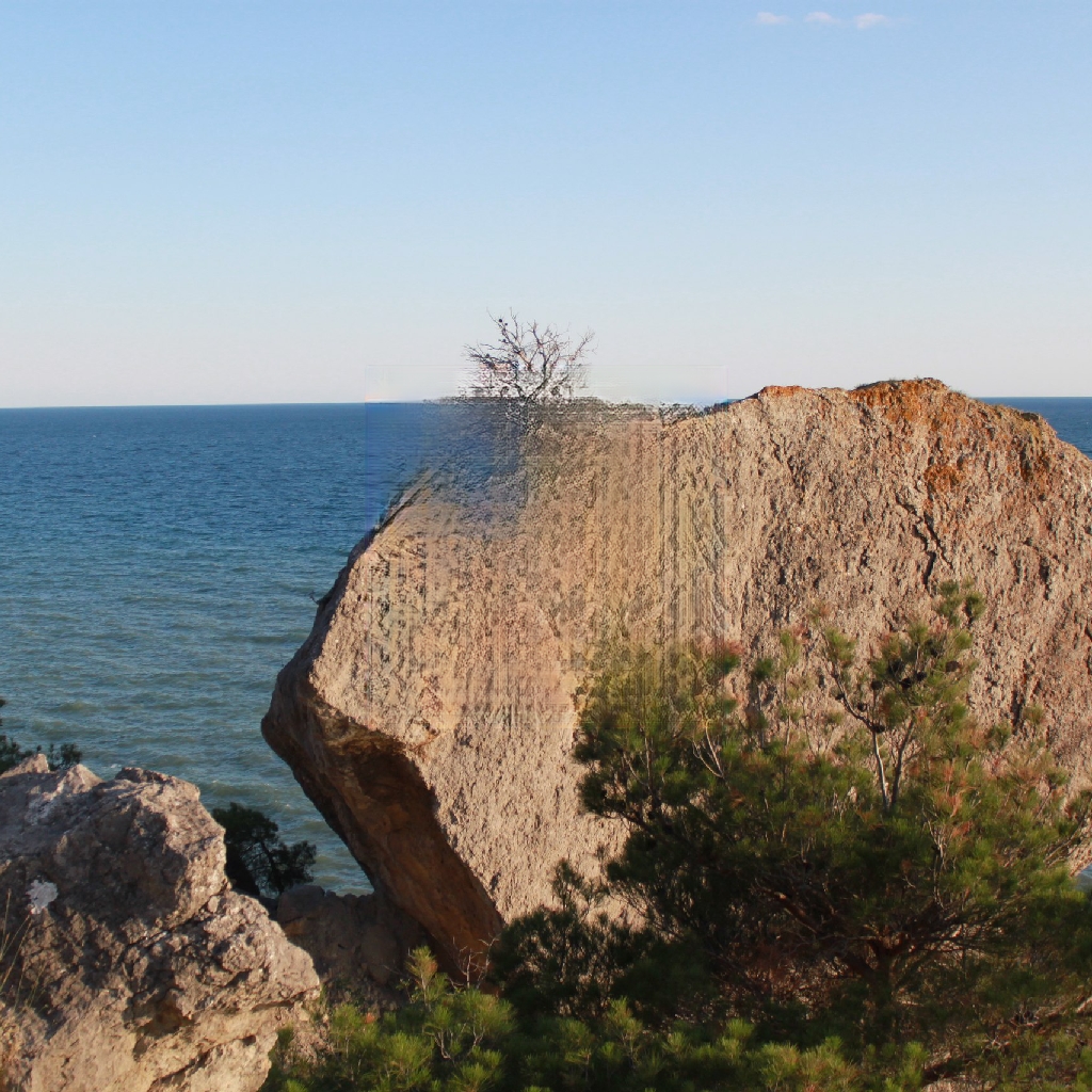
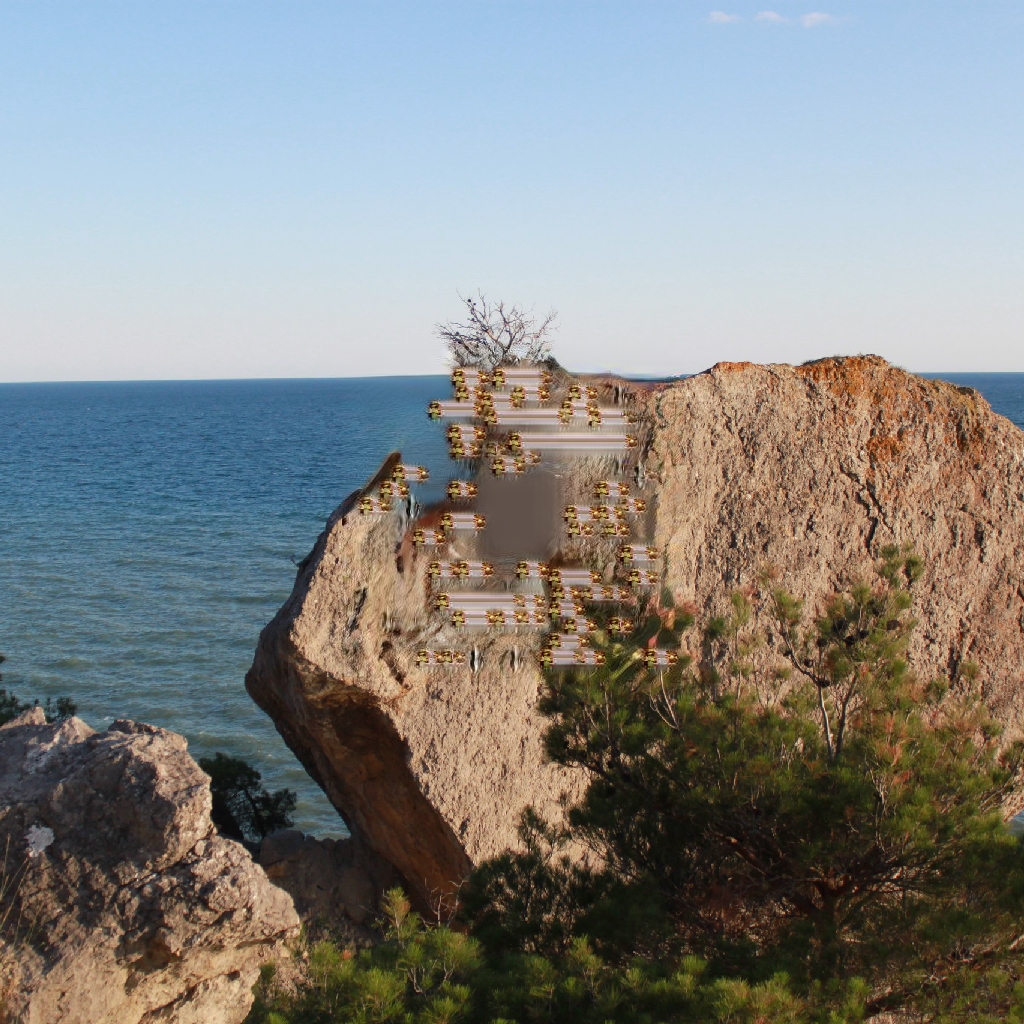
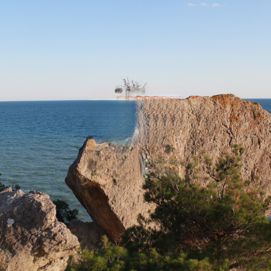
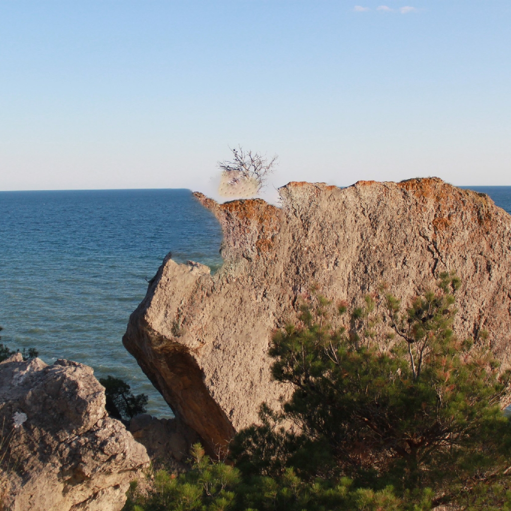
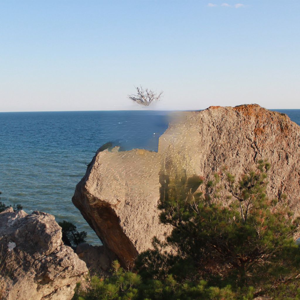
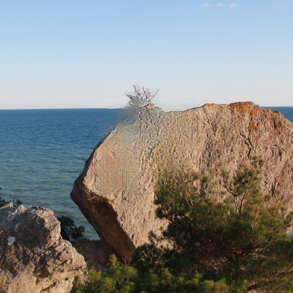
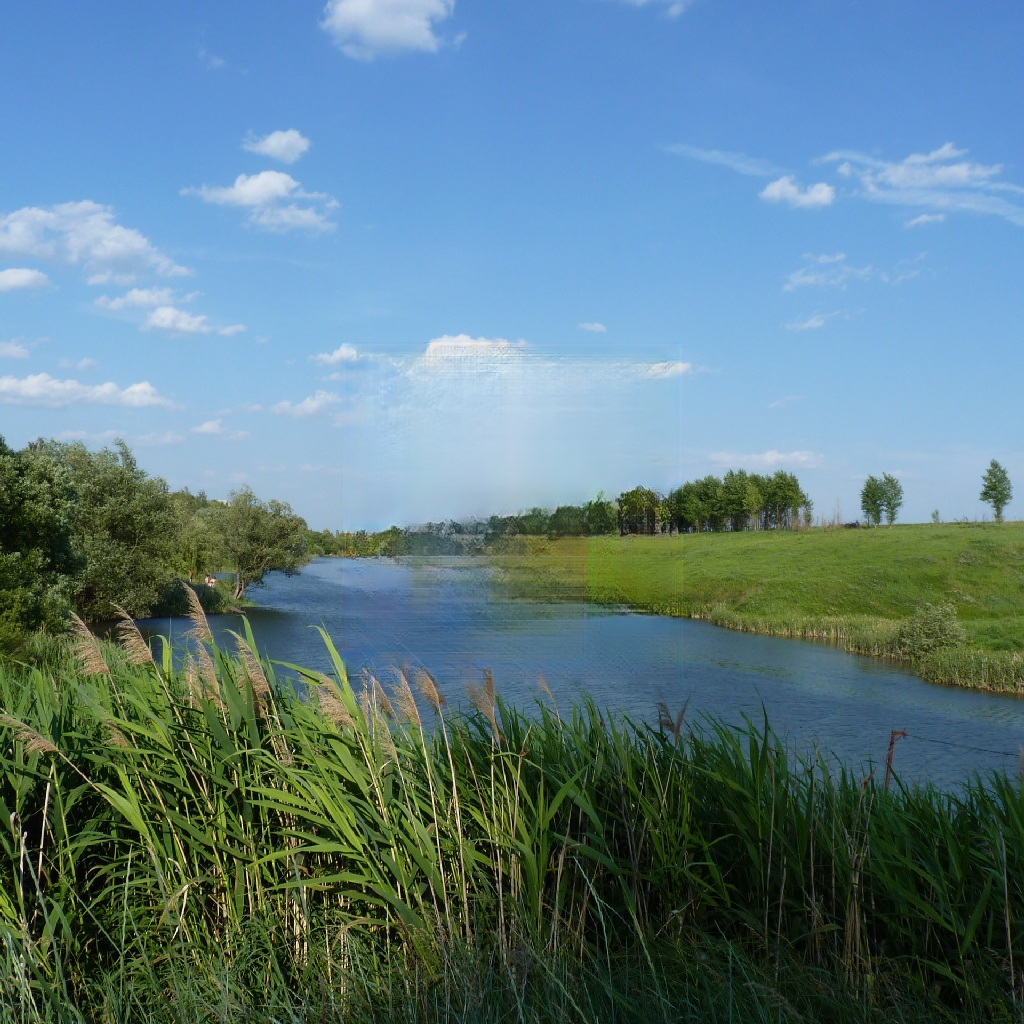
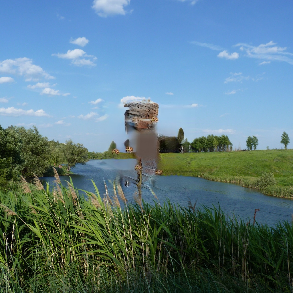
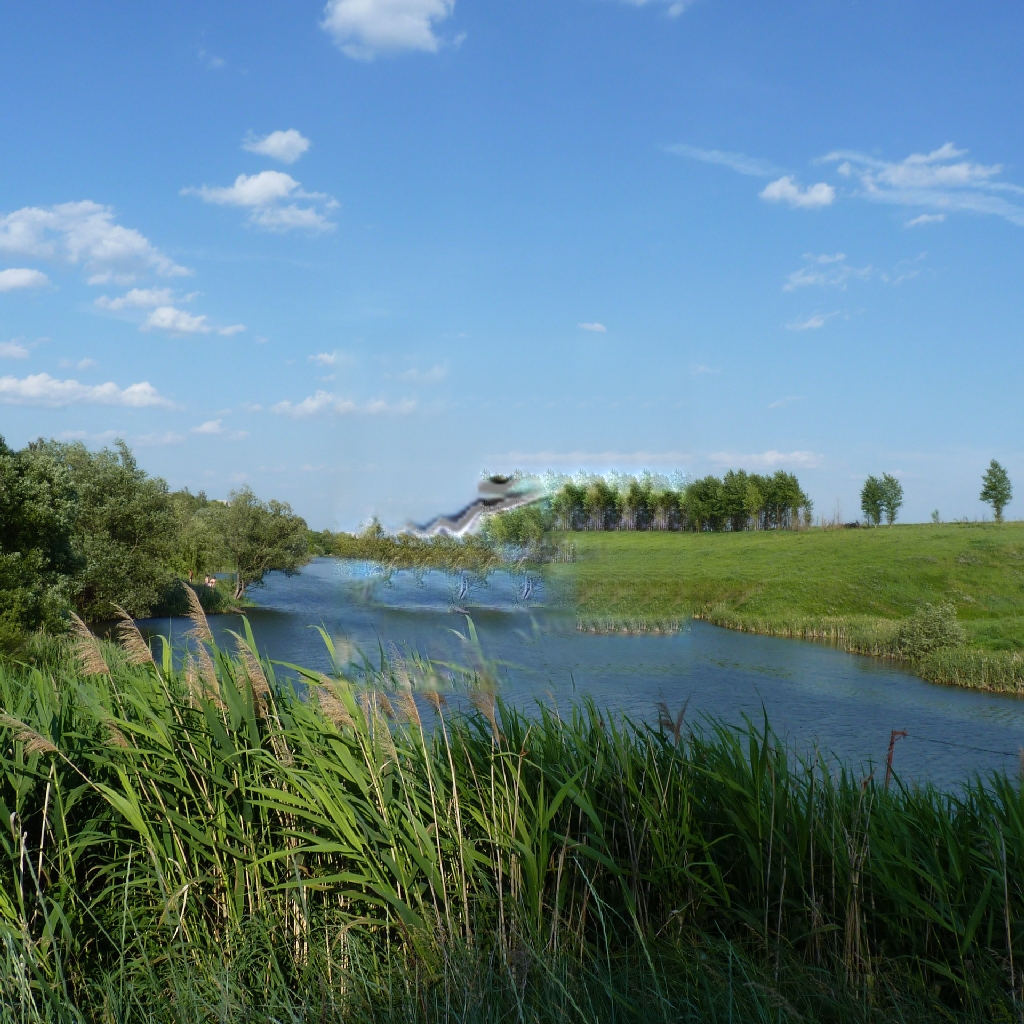
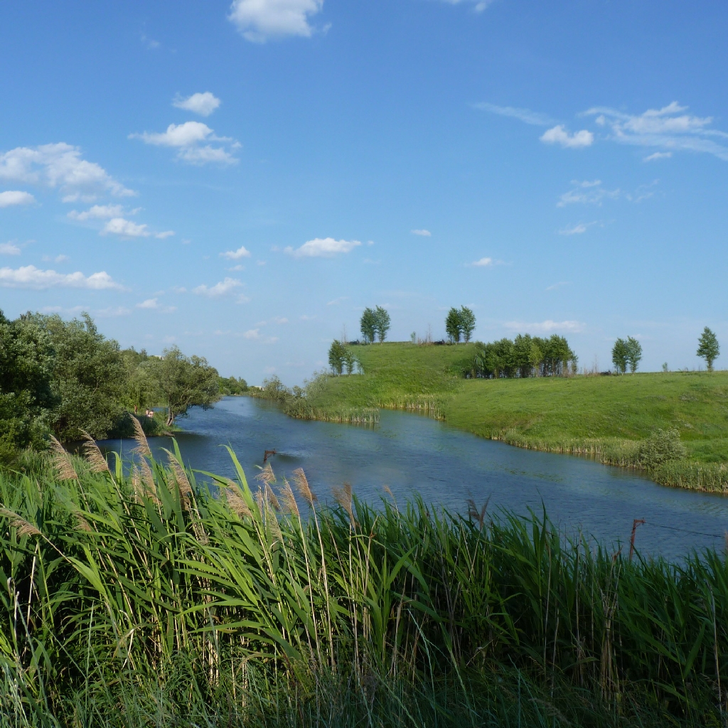
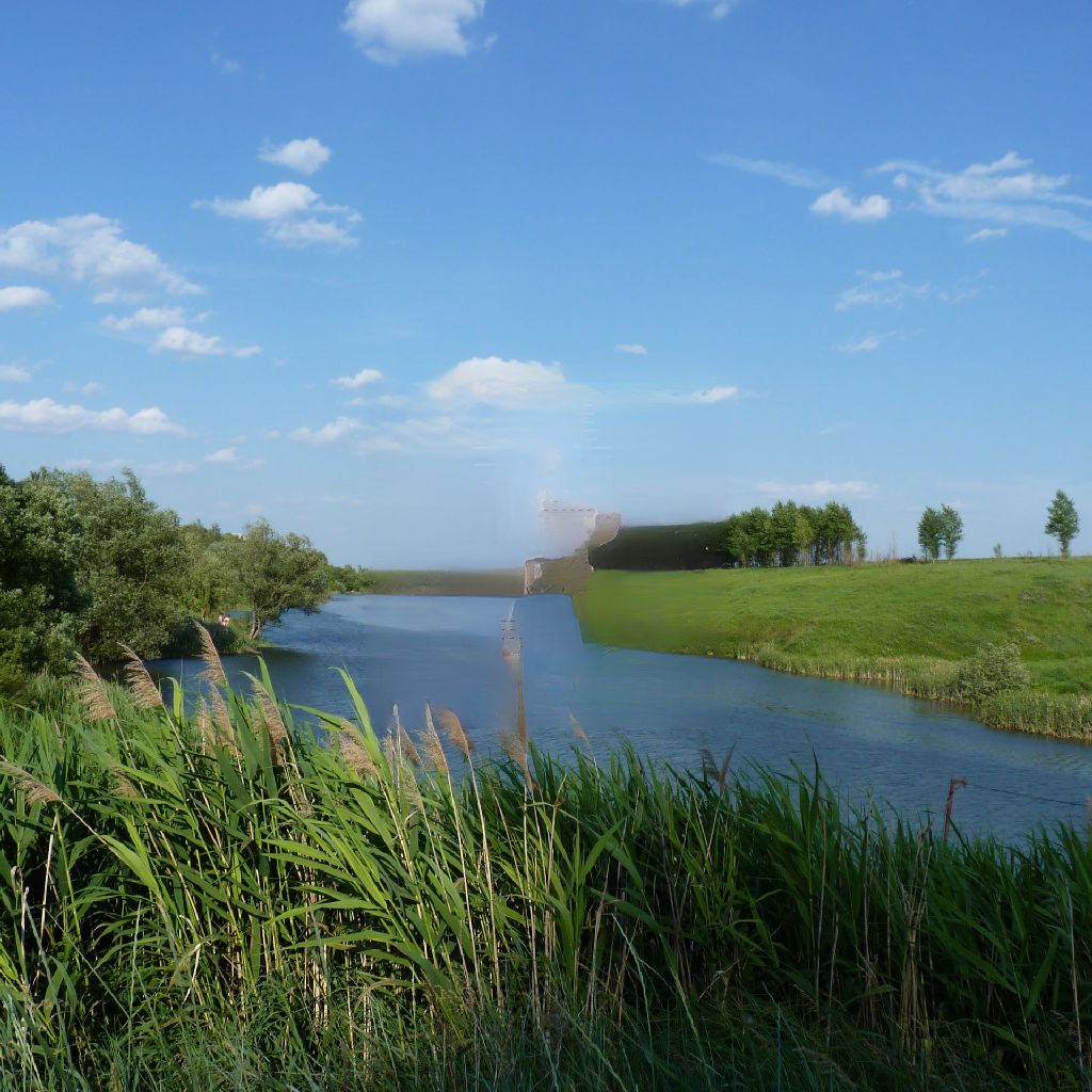
DFNet	DeepFillv2	HiFill	Photoshop	ProFill	Ours

Figure 4: Methods outputs with ${1024\times 1024}$ images

4.1 Comparisons

Fig. 1, Fig. 4, and Fig. 7 show examples of our work. Although the method functions almost identically at any resolution, we limited ourselves to ${1024\times 1024}$. More pictures and resolutions appear in the repository.

Figure 5: Subjective comparison scores (resolution 2048x2048)

Figure 6: Subjective comparison scores (resolution 1024x1024)

4.1.1 Subjective evaluation

To conduct a subjective evaluation, we selected a set of 34 natural images mostly from [7] with a full resolution of ${2048\times 2048}$. Participants were shown two images and asked to choose the one with the highest visual quality. We also added two validation questions to exclude unscrupulous viewers. Due to the implementation limitations of the [12] we made two separate comparisons at ${2048\times 2048}$ and ${1024\times 1024}$ resolutions. In first comparison 150 people participated, yielding 3,750 valid votes. In second comparison 248 people participated, yielding 6200 valid votes. Then paired estimates were converted into numerical ones using [19] model. The results appear in Fig. 5, Fig. 6.

4.1.2 Objective evaluation

Due to the complexity of subjective evaluation, we only conducted objective comparisons for other resolutions, although this may not be confirmed by observers ratings. For the objective comparison, we also added output images from Adobe Photoshop 2020, a commercial package that implements the classical inpainting approach. Our quality metrics were the mean L1 distance, SSIM [20], and PSNR. To reduce resolution, we used Nearest-Neighbor downsampling. Table 1 shows the results for this objective comparison.

Table 1: Objective comparison with different resolutions

	L1	PSNR	SSIM		L1	PSNR	SSIM
DeepFill v2	4.981	22.389	0.938		5.397	21.956	0.944
DFNet	3.592	24.910	0.946		4.132	23.836	0.946
HiFill	4.422	23.667	0.935		4.373	23.738	0.943
Photoshop 2020	4.115	23.789	0.944		13.320	23.756	0.949
ProFill	3.906	24.677	0.950		—	—	—
Ours	3.524	25.175	0.944		3.474	25.311	0.950
Resolution	1024x1024				1536x1536
	L1	PSNR	SSIM		L1	PSNR	SSIM
DeepFill v2	5.546	21.834	0.946		5.669	21.697	0.948
DFNet	4.345	23.424	0.948		4.633	22.915	0.950
HiFill	4.403	23.696	0.944		4.391	23.710	0.947
Photoshop 2020	4.047	23.863	0.952		4.153	23.659	0.952
Ours	3.447	25.374	0.952		3.434	25.412	0.954
Resolution	1792x1792				2048x2048

4.2 GIMP Plugin

Inspired by [21], we embedded our method in the GNU Image Manipulation Program (GIMP). The final plugin, which implements our method, appears in the repository.

5 Conclusion

This work proposes an inpainting technique that handles images of different sizes. We conducted both objective and subjective comparisons with existing learning-based models and a popular commercial package, showing that our method produces a more satisfactory result. Also, our approach can theoretically apply to any inpainting model, making it resolution independent. In the future, we would like to train a new model using the proposed method, but in an end-to-end manner with dynamic shift size.

5.0.1 Acknowledgments

This work was partially supported by Russian Foundation for Basic Research under Grant 19-01-00785 a. Model training for this work employed the IBM Polus computing cluster of the Faculty of Computational Mathematics and Cybernetics at Moscow State University.

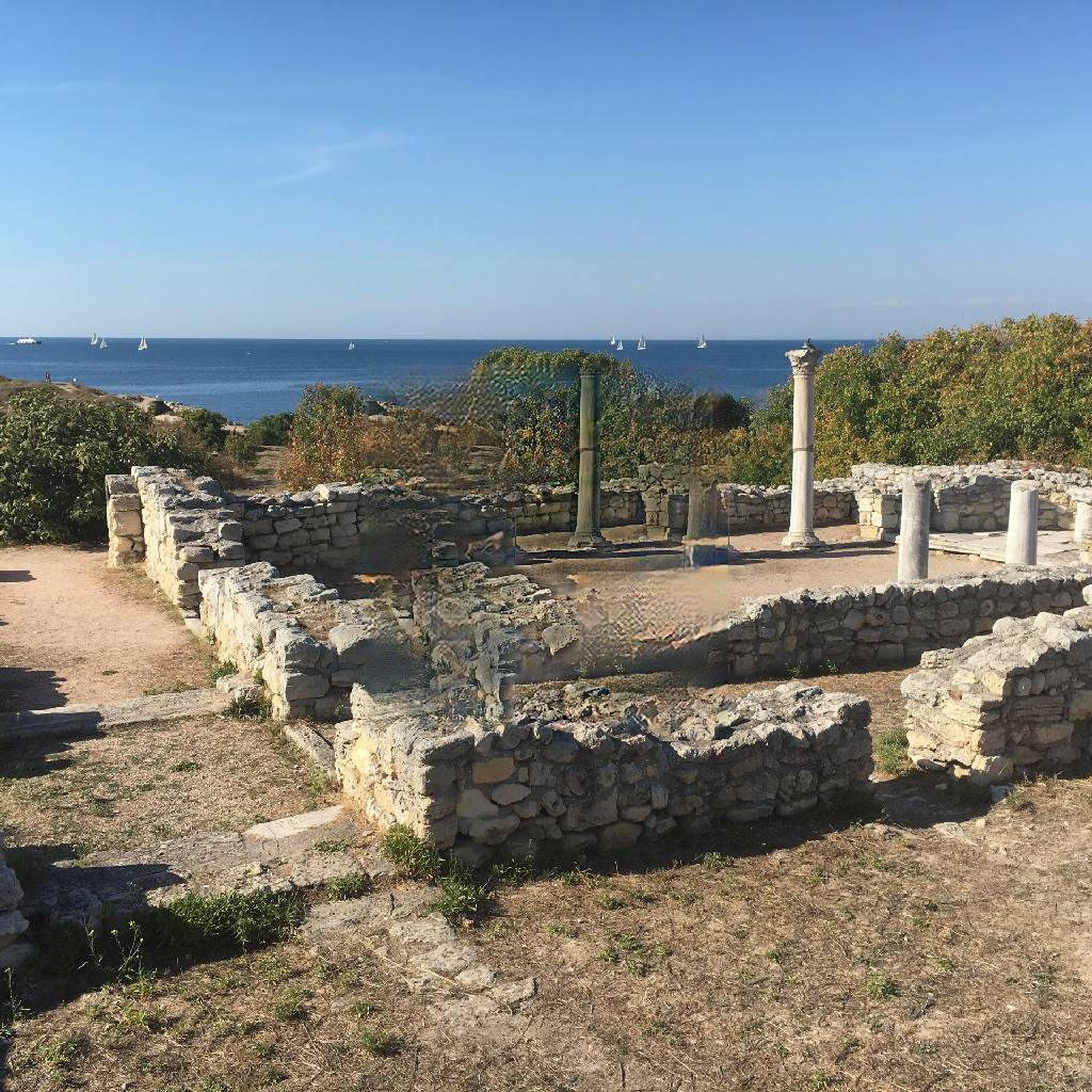
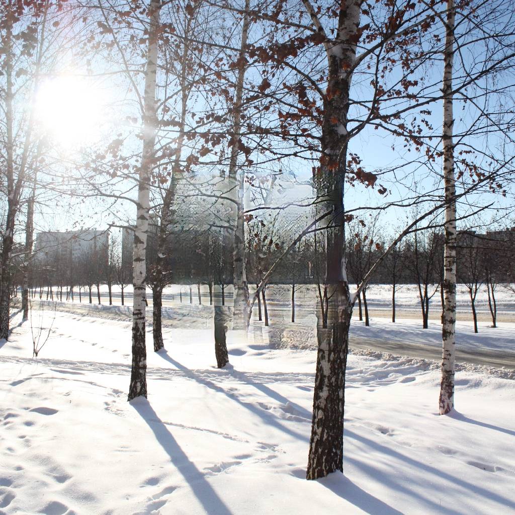
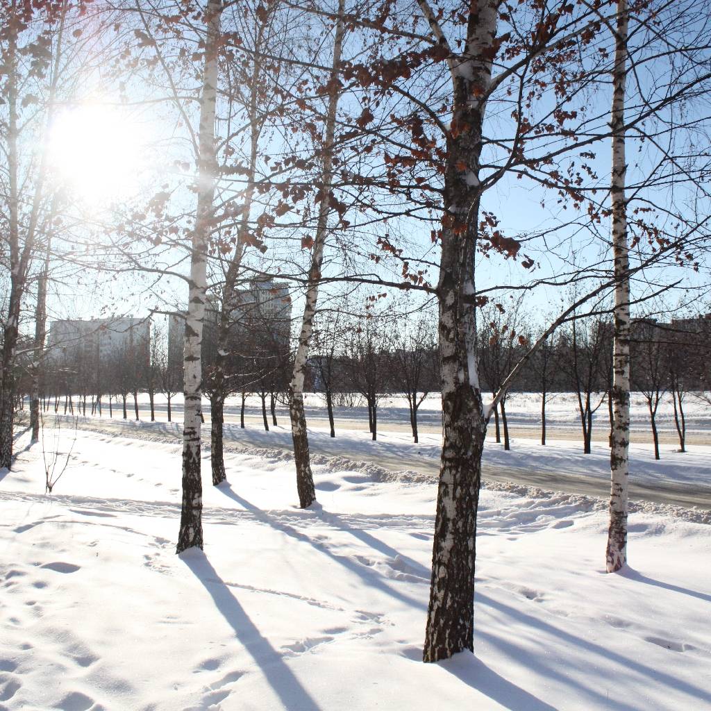
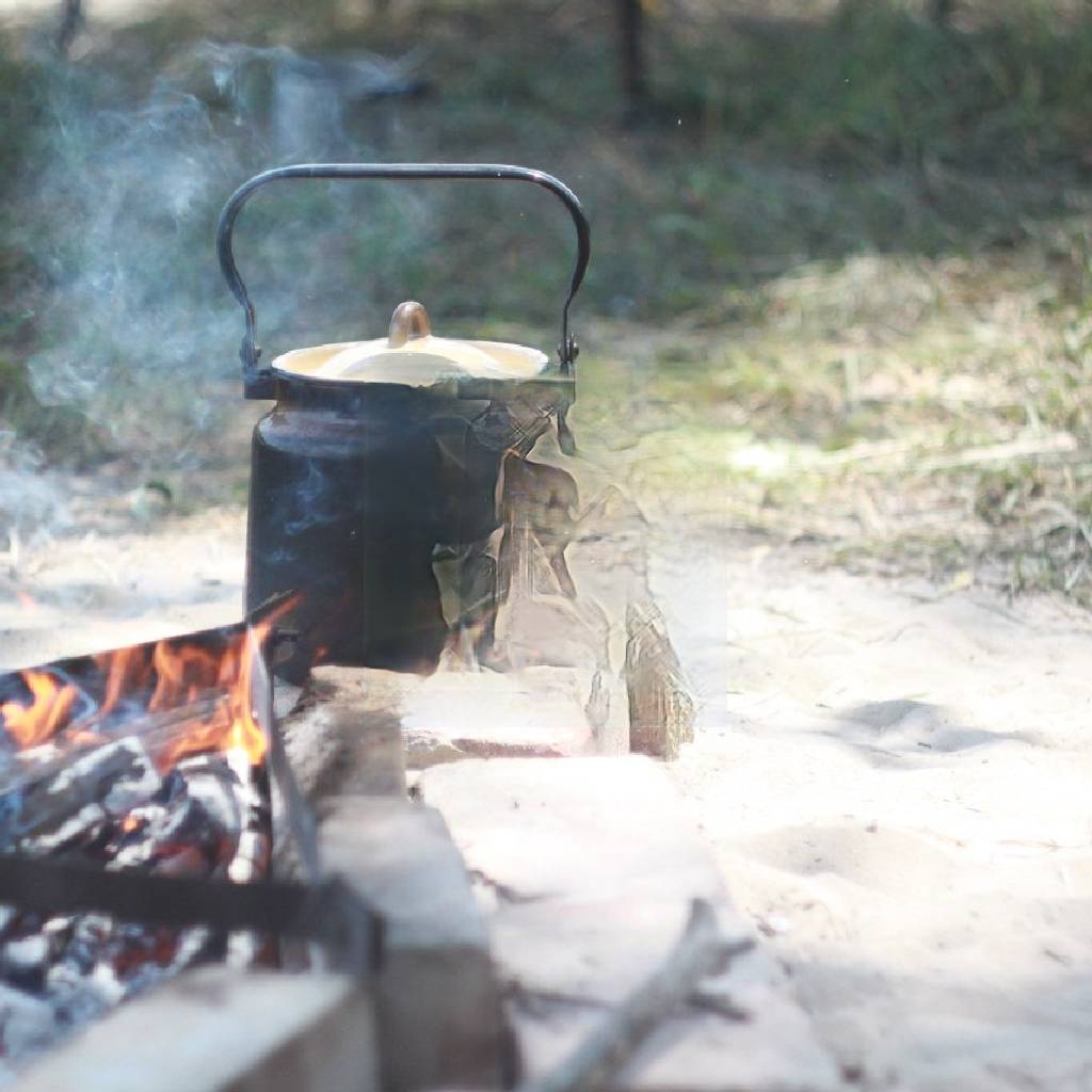
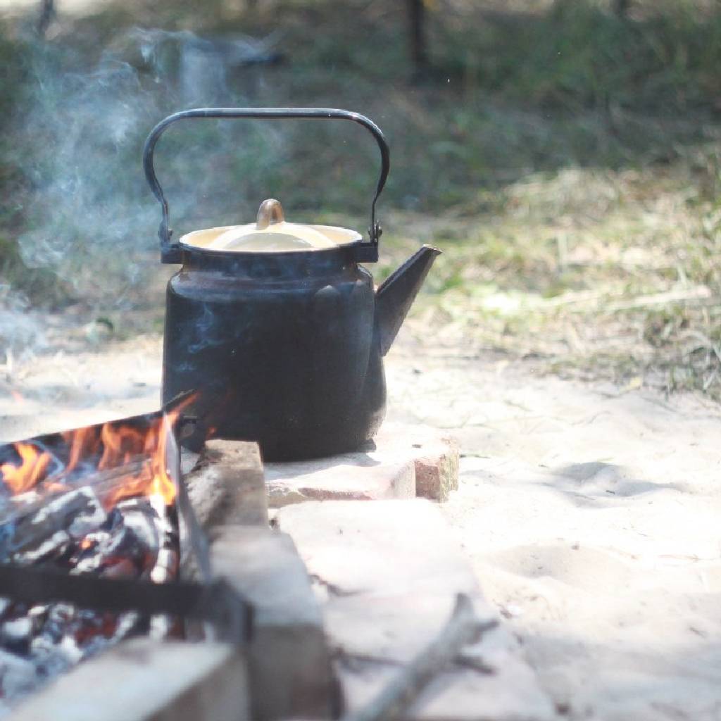
Ours	GT	Ours	GT

Figure 7: Failures of our model

References

- [1] Drori, I., Cohen-Or, D., Yeshurun, H.: Fragment-based image completion. ACM Transactions on Graphics 22 (08 2003)
- [2] Criminisi, A., Perez, P., Toyama, K.: Region filling and object removal by exemplar-based image inpainting. IEEE Transactions on Image Processing 13(9), 1200–1212 (2004)
- [3] Barnes, C., Shechtman, E., Finkelstein, A., Goldman, D.: Patchmatch: A randomized correspondence algorithm for structural image editing. ACM Trans. Graph. 28 (08 2009)
- [4] Liu, G., Reda, F.A., Shih, K.J., Wang, T.C., Tao, A., Catanzaro, B.: Image inpainting for irregular holes using partial convolutions. In: The European Conference on Computer Vision (ECCV) (2018)
- [5] Yu, J., Lin, Z., Yang, J., Shen, X., Lu, X., Huang, T.S.: Generative image inpainting with contextual attention. 2018 IEEE/CVF Conference on Computer Vision and Pattern Recognition (Jun 2018)
- [6] Hong, X., Xiong, P., Ji, R., Fan, H.: Deep fusion network for image completion. In: Proceedings of the 27th ACM International Conference on Multimedia. pp. 2033–2042. MM ’19, ACM, New York, NY, USA (2019)
- [7] Molodetskikh, I., Erofeev, M., Vatolin, D.: Perceptually motivated method for image inpainting comparison (2019)
- [8] Goodfellow, I., Pouget-Abadie, J., Mirza, M., Xu, B., Warde-Farley, D., Ozair, S., Courville, A., Bengio, Y.: Generative adversarial nets. ArXiv (06 2014)
- [9] Iizuka, S., Simo-Serra, E., Ishikawa, H.: Globally and locally consistent image completion. ACM Transactions on Graphics 36, 1–14 (07 2017)
- [10] Yu, J., Lin, Z., Yang, J., Shen, X., Lu, X., Huang, T.: Free-form image inpainting with gated convolution. 2019 IEEE/CVF International Conference on Computer Vision (ICCV) (Oct 2019)
- [11] Yi, Z., Tang, Q., Azizi, S., Jang, D., Xu, Z.: Contextual residual aggregation for ultra high-resolution image inpainting (2020)
- [12] Zeng, Y., Lin, Z., Yang, J., Zhang, J., Shechtman, E., Lu, H.: High-resolution image inpainting with iterative confidence feedback and guided upsampling. In: European Conference on Computer Vision. pp. 1–17. Springer (2020)
- [13] Ronneberger, O., Fischer, P., Brox, T.: U-net: Convolutional networks for biomedical image segmentation. Medical Image Computing and Computer-Assisted Intervention – MICCAI 2015 p. 234–241 (2015)
- [14] Simonyan, K., Zisserman, A.: Very deep convolutional networks for large-scale image recognition. arXiv 1409.1556 (09 2014)
- [15] Timofte, R., Gu, S., Wu, J., Van Gool, L., Zhang, L., Yang, M.H., Haris, M., et al.: Ntire 2018 challenge on single image super-resolution: Methods and results. In: The IEEE Conference on Computer Vision and Pattern Recognition (CVPR) Workshops (June 2018)
- [16] Ioffe, S., Szegedy, C.: Batch normalization: Accelerating deep network training by reducing internal covariate shift (2015)
- [17] Johnson, J., Alahi, A., Fei-Fei, L.: Perceptual losses for real-time style transfer and super-resolution. Lecture Notes in Computer Science p. 694–711 (2016)
- [18] Kingma, D.P., Ba, J.: Adam: A method for stochastic optimization (2014)
- [19] Bradley, R.A., Terry, M.E.: Rank analysis of incomplete block designs: I. the method of paired comparisons. Biometrika 39(3/4), 324–345 (1952)
- [20] Wang, Z., Bovik, A., Sheikh, H., Simoncelli, E.: Image quality assessment: From error visibility to structural similarity. Image Processing, IEEE Transactions on 13, 600 – 612 (05 2004)
- [21] Soman, K.: Gimp-ml: Python plugins for using computer vision models in gimp. arXiv preprint arXiv:2004.13060 (2020)