Transverse momentum dependent parton densities in processes with heavy quark generations

Abstract

To study the heavy quark production processes, we use the transverse momentum dependent (TMD, or unintegrated) gluon distribution function in a proton obtained recently using the Kimber-Martin-Ryskin prescription from the Bessel-inspired behavior of parton densities at small Bjorken $x$ values. We obtained a good agreement of our results with the latest HERA experimental data for reduced cross sections $\sigma^{c\overline{c}}_{\rm red}(x,Q^{2})$ and $\sigma^{b\overline{b}}_{\rm red}(x,Q^{2})$, and also for deep inelastic structure functions $F_{2}^{c}(x,Q^{2})$ and $F_{2}^{b}(x,Q^{2})$ in a wide range of $x$ and $Q^{2}$ values. Comparisons with the predictions based on the Ciafaloni-Catani-Fiorani-Marchesini evolution equation and with the results of conventional pQCD calculations performed at first three orders of perturbative expansion are presented.

Keywords: small $x$, QCD evolution, TMD parton densities, high energy factorization

1 Introduction

Recently, important new data have appeared on the cross sections for the open charm and beauty production in neutral current deep inelastic electron-proton scattering (DIS) obtained[1] by combining the results of H1 and ZEUS Collaborations at HERA. Measurements have shown that heavy flavour production in DIS proceeds predominantly via the photon-gluon fusion process, $\gamma g\to Q\overline{Q}$, where $Q$ is the heavy quark. The cross section therefore depends strongly on the gluon distribution in the proton and heavy quark mass. Moreover, an analysis of the data in the framework of perturbative Quantum Chromodynamics (QCD) has been done[1], where the massive fixed-flavour-number scheme and different implementations of the variable-flavour-number scheme were used.

The theoretical description of the heavy quark production processes can also be performed with transverse momentum dependent (TMD), or non-integrated, functions of the density of partons (quarks and/or gluons) in a proton [2, 3]. These quantities, depending on the fraction of the longitudinal momentum $x$ of the proton carried by the parton, the two-dimensional transverse momentum of the parton ${\mathbf{k}_{T}^{2}}$, and the hard scale $\mu^{2}$ of a complex process, contain nonperturbative information about the proton structure, including the transverse momentum. The TMD factorization theorems provide the necessary basis for separating hard parton physics, described in terms of perturbative QCD, and soft hadron physics. Currently, there are a number of factorization approaches that include the dependence of the parton distribution fnctions (PDFs) on the transverse momentum: for example, the Collins-Soper-Sterman [4] approach, developed for semi-inclusive processes with a finite and nonzero ratio between the rigid scale $\mu^{2}$ and total energy $s$, as well as the approach to high-energy factorization [5, 6] (or $k_{T}$-factorization [7]), valid at a fixed limit of the hard scale and at high energies.

With high-energy factorization, the TMD density of gluons satisfies the Balitsky-Fadin-Kuraev-Lipatov (BFKL) [8] or Ciafaloni-Catani-Fiorani-Marchesini (CCFM) [9] evolution equations, which resum the contributions of large logarithms proportional to $\alpha_{s}^{n}\ln^{n}s\sim\alpha_{s}^{n}\ln^{n}1/x$. These terms are important at high energies $s$ (or, equivalently, at low $x$ values). Thus, high-order radiative corrections can be effectively taken into account in the estimated cross sections (namely, the part of the next-to-leading order (NLO) + of the next-to-leading order (NNLO) + … terms corresponding to the emission of the original gluons). Phenomenological applications of the high-energy factorization approach augmented by the CCFM are well known in the literature (see, for example, [10, 11, 12, 13, 14, 15, 16, 17, 18, 19, 20] and references therein).

In addition to the CCFM equation, there are also other approaches to determining the TMD PDFs in a proton. They can be estimated using schemes based on the usual Dokshitser-Gribov-Lipatov-Altarelli-Parisi (DGLAP) [21] equations, namely the parton branching approach (PB) [22] and the Kimber-Martin-Ryskin (KMR) recipe [23]. The first of them gives a numerical iterative solution of the DGLAP evolution equations for collinear and TMD PDFs using the concept of resolvable and non-resolvable branching and the application of Sudakov’s formalism to describe the evolution of a parton from one scale to another without decidable branching. The splitting kinematics at each branching vertex is described by the DGLAP equations and the angular ordering condition for parton emission, which can be used instead of the usual DGLAP ordering by virtuality. The KMR approach is a formalism invented to construct TMD PDFs from well-known traditional (collinear) PDFs under the key assumption that the dependence of parton distributions on transverse momentum comes only in the last stage of evolution. It is believed that the KMR procedure effectively takes into account a main part of the following next-to-leading logarithmic (NLL) terms $\alpha_{s}(\alpha_{s}\ln\mu^{2})^{n-1}$ compared to the leading logarithmic approximation (LLA), where terms are proportional to $\alpha_{s}^{n}\ln^{n}\mu^{2}$ taken into account only. The KMR approach is currently being explored in NLO [24] and is commonly used in phenomenological applications (see, for example, [11, 13, 14, 15, 16, 17, 18, 19] and references therein), where the usual PDFs (for example, the NNPDF [25] or CTEQ [26] ones) accepted numerically as input. The relationship between PB and KMR scenarios has been discussed [27], and the relationship between PB and CCFM approaches has been recently created [28].

The KMR formalism was used in our recent article [29] for analytical calculations of the TMD PDFs. These calculations are based on the [30, 31, 32] expressions for usual PDFs obtained with the generalized double asymptotic scaling (DAS) approach [33, 31, 32]. This scaling, related to the asymptotic behavior of DGLAP evolution, was discovered many years ago by [34]. It was shown [30, 31, 32] that the flat initial conditions for the DGLAP equations used in the generalized DAS scheme lead to the Bessel-like behavior of PDFs at small $x$ values. Using the results [30, 31, 32], analytical expressions for the TMD quark and gluon densities has be obtained [29] in the leading order (LO) . In Ref. [29], we have implemented various kinematic constraints that exist in the KMR recipe (namely, angular and strict ordering conditions), and investigated the relationship between the differential and integral formulations of the KMR procedure recently mentioned in [36].

In the present paper we continue our investigations and analyze the combined H1 and ZEUS experimental data [1] for the (reduced) charm and beauty cross sections $\sigma^{c\overline{c}}_{\rm red}$ and $\sigma^{b\overline{b}}_{\rm red}$ and charm and beauty contributions to the proton structure functions (SFs) $F_{2}(x,Q^{2})$ and $F_{L}(x,Q^{2})$[37, 38, 39] and their ratio for different $Q^{2}$ values. Studying the earlier data on the charm SF $F^{c}_{2}$ in the proton from H1[40] and ZEUS[41] Collaborations at HERA, obtained for $x\sim 10^{-4}$, it was found that the charm contribution to the total proton SF $F_{2}$ is about 25$\%$, which is significantly larger than that found by the European Muon Collaboration at CERN[42] for large $x$, where SF $F^{c}_{2}$ was only $1\%$ of $F_{2}$. Such a large value of $F^{c}_{2}$ required extensive experimental and theoretical studies of heavy quark production processes (see, for example, the data [1] studied in this paper, as well as the experimental data[43] from LHCb Coolaboration at CERN for the prompt charm production in $pp$ collisions). Theoretical studies usually serve to confirm that HERA and LHC data can be described by perturbative charm generation within QCD (see, for example, reviews[44, 45, 46] and references therein). We also note here that, historically, it was in the study of these processes that the $k_{T}$-factorization was introduced and tested (see[5, 6, 7]).

The production of charmed mesons ah hadron colliders is dominated by the $gg\to c\overline{c}$ subprocess, and therefore it provides a sensitive probe of the gluon density at small $x$. In particular the data[43] of LHCb Collaboration provides an information on the gluon at values of $x$ as small as $x\sim 10^{-6}$ (see[47] and discussions therein). This very small-$x$ region is also crucial for the calculations of signal and backgroud processes for ultra-high energy neutrino astrophysics (see[48] and [49] for calculations of the high energy neutrino cross-section and the prompt atmospheric neutrino flux, respectively). A study of the heavy quark production will be contitued at future lepton-hadron and hadron-hadron colliders, such as LHeC, FCC-eh and FCC-hh, respectively (for a review, see[50, 51] and references therein).

To study the process of the heavy quark production, we produce the $k_{T}$-factorization predictions in two ways, namely, using the framework of DAS approach and CCFM evolution equation. The direct comparison of these predictions is interesting and could be rather useful to discriminate between the different approaches to evaluate the TMD parton (mainly gluon) density in a proton. Then, we calculate the high-energy asymptotics of the heavy quark parts of the SFs $F_{2}$ and $F_{L}$ at first three orders of perturbation theory and present the numerical comparison of these higher-order predictions with corresponding results of the $k_{T}$-factorization calculations.

The outline of our paper is following. In Sections 2 and 3 we briefly describe our theoretical input. Section 4 presents our numerical results for the reduced charm and beauty cross sections and charm and beauty parts of SFs $F_{2}(x,Q^{2})$ and $F_{L}(x,Q^{2})$ in a wide $Q^{2}$ range. Section 5 contains our conclusions. In Appendix A we present the high energy asymptotics of the heavy quark contribution to the SFs $F_{2}$ and $F_{L}$ at first three orders of perturbation theory. Appendix B contains the simple approximations of these formulas for the ratio of the heavy quark parts of the SFs $F_{2}$ and $F_{L}$, which could be useful for subsequent applications.

2 $k_{T}$-dependent Wilson coefficient functions

The differential cross section $\sigma^{Q\bar{Q}}$ (hereafter $Q=c,b$) can be presented in the simple form:

$${d^{2}\sigma^{Q\bar{Q}}\over dxdy}={2\pi\alpha^{2}\over xQ^{4}}\left[\left(1-y+{y^{2}\over 2}\right)F_{2}^{Q}(x,Q^{2})-{y^{2}\over 2}F_{L}^{Q}(x,Q^{2})\right],$$ (1)

where $F_{k}^{Q}(x,Q^{2})$ (hereafter $k=2,L$) are heavy quark parts of the proton SFs $F_{k}(x,Q^{2})$, $x$ and $y$ are the usual Bjorken scaling variables. Here we present the basic elements of the relations between SFs $F_{2}^{Q}(x,Q^{2})$ and $F_{L}^{Q}(x,Q^{2})$ and TMD PDFs. More detail analysis can be found in[52].

In the $k_{T}$-factorization approach, the SFs $F^{Q}_{k}(x,Q^{2})$ are driven at small $x$ by gluons and related in the following way to the TMD gluon distribution $f_{g}(x,{\mathbf{k}}^{2}_{T},\mu^{2})$:

$$F^{Q}_{k}(x,Q^{2})=\int^{1}_{x}\frac{dx^{\prime}}{x^{\prime}}\int\frac{dk^{2}_{\bot}}{k^{2}_{\bot}}\;C_{k,g}(x,Q^{2},m^{2},k^{2}_{\bot},\mu^{2})~{}f_{g}\left(\frac{x}{x^{\prime}},k^{2}_{\bot},\mu^{2}\right).$$ (2)

The functions $C_{k,g}(x,Q^{2},m_{f}^{2},k^{2}_{\bot},\mu^{2})$ may be regarded as the structure functions of the off-shell gluons with virtuality $k^{2}_{\bot}$ (hereafter we call them as Wilson coefficient functions). Following[52], we do not use the Sudakov decomposition, which is sometimes quite convenient in high-energy calculations. Here we only note that the property $k^{2}=-k^{2}_{\bot}$ comes from the fact that the Bjorken parton variable $x$ in the standard and in the Sudakov approaches coincide.

The $k_{\bot}$-dependent Wilson coefficient functions have the following form:

$$C_{k,g}(x)=\frac{1}{\tilde{\beta}^{4}}\left[\tilde{\beta}^{2}\overline{C}_{k,g}(x)-12bx^{2}\frac{q^{\alpha}q^{\beta}}{Q^{2}}\tilde{C}_{k,g}(x)\right],~{}~{}$$ (3)

where $\overline{C}_{k,g}(x)$ and $\tilde{C}_{k,g}(x)$ corresponds to application of the Feynman $P_{F}^{\alpha\beta}$ polarization tensor and additional tensor of gluon polarization $P_{a}^{\alpha\beta}$:

$$\hat{P}_{F}^{\alpha\beta}=-\frac{1}{2}\,g^{\alpha\beta},~{}~{}\hat{P}_{a}^{\alpha\beta}=\frac{6bx^{2}}{\tilde{\beta}^{2}}\,\frac{q^{\alpha}q^{\beta}}{Q^{2}}.$$ (4)

Hereafter

$$\tilde{\beta}^{2}=1-4bx^{2},~{}~{}b=-\frac{k^{2}}{Q^{2}}\equiv\frac{k_{\bot}^{2}}{Q^{2}},~{}~{}a=\frac{m^{2}}{Q^{2}},~{}~{}Q^{2}>0,\,$$ (5)

and we omitted the dependence of the coefficient functions on the heavy quark mass $m$, $Q^{2}$, $k^{2}_{\bot}$ and hard scale $\mu^{2}$. The sum of the polarizations tensors produces so-called BFKL polarizations tensor:

$$\hat{P}^{\alpha\beta}_{BFKL}=\frac{k_{\bot}^{\alpha}k_{\bot}^{\beta}}{k_{\bot}^{2}}=\frac{x^{2}}{-k^{2}}p^{\alpha}p^{\beta}.~{}~{}~{}$$ (6)

Indeed, as it was shown in[52]

$$\hat{P}^{\alpha\beta}_{BFKL}~{}=~{}-\frac{1}{2}\frac{1}{\tilde{\beta}^{4}}\left[\tilde{\beta}^{2}g^{\alpha\beta}-12bx^{2}\frac{q^{\alpha}q^{\beta}}{Q^{2}}\right]=\hat{P}_{F}^{\alpha\beta}+\hat{P}_{a}^{\alpha\beta}\,.$$ (7)

After applying the photon polarizations tensors

$$\hat{P}^{(1)}_{\mu\nu}=-\frac{1}{2}g_{\mu\nu}~{}~{}\mbox{ and }~{}~{}\hat{P}^{(2)}_{\mu\nu}=4x^{2}\frac{k_{\mu}k_{\nu}}{Q^{2}}\,,$$ (8)

which can be rewritten as

$$P^{(i)}_{\mu\nu}F_{\mu\nu}=\frac{e_{f}^{2}a_{s}}{\beta^{2}}\;f^{(i)},\,i=1,2\,,$$ (9)

the results for the coefficient functions $C_{k,2}(x)$ have been calculated in [52]:

$$C_{2,g}(x) = \frac{e_{Q}^{2}a_{s}}{\beta^{2}}\;\left[f^{(1)}+\frac{3}{2\tilde{\beta}^{2}}\;f^{(2)}\right]\,\Theta(x_{1}-x)$$ (10)

$$C_{L,g}(x) = \frac{e_{Q}^{2}a_{s}}{\beta^{2}}\;\left[4bx^{2}f^{(1)}+\frac{(1+2bx^{2})}{\tilde{\beta}^{2}}\;f^{(2)}\right]\,\Theta(x_{1}-x)$$ (11)

$$= \frac{e_{Q}^{2}a_{s}}{\beta^{2}}\;f^{(2)}\,\Theta(x_{0}-x)+4bx^{2}\,C^{g}_{2},$$

where $a_{s}=\alpha_{s}/(4\pi)$ is the strong coupling constant, $\Theta(x_{1}-x)$ is the Heaviside step function and

$$x_{1}~{}=~{}\frac{1}{1+4a+b}\,.$$ (12)

Following to the representation (7) of gluon polarization tensors, we can represent the basic functions $f^{(i)}$ $(1,2)$ in the following form:

$$f^{(i)}=\frac{1}{\tilde{\beta}^{4}}\left[\tilde{\beta}^{2}\overline{f}^{(i)}~{}-~{}3bx^{2}\tilde{f}^{(i)}\right]\,,$$ (13)

where

$$\overline{f}^{(1)} = -2\overline{\beta}\Biggl{[}1-\biggl{(}1-2x(1+b-2a)\;[1-x(1+b+2a)]\biggr{)}\;f_{1}$$ (14)

$$+ (2a-b)(1-2a)x^{2}\;f_{2}\Biggr{]},$$

$$\overline{f}^{(2)} = 8x\;\overline{\beta}\Biggl{[}(1-(1+b)x)-2x\biggl{(}bx(1-(1+b)x)(1+b-2a)+a\tilde{\beta}^{2}\biggr{)}\;f_{1}$$ (15)

$$+ bx^{2}(1-(1+b)x)(2a-b)\;f_{2}\Biggr{]}$$

and

$$\tilde{f}^{(1)} = -\overline{\beta}\Biggl{[}\frac{1-x(1+b)}{x}-2\biggl{(}x(1-x(1+b))(1+b-2a)+a\tilde{\beta}^{2}\biggr{)}\;f_{1}$$ (16)

$$- x(1-x(1+b))(1-2a)\;f_{2}\Biggr{]},$$

$$\tilde{f}^{(2)} = 4\;\overline{\beta}~{}(1-(1+b)x)^{2}\Biggl{[}2-(1+2bx^{2})\;f_{1}-bx^{2}\;f_{2}\Biggr{]}.$$ (17)

Here

$$\overline{\beta}^{2}=1-\frac{4ax}{(1-(1+b)x)}$$ (18)

and

$$f_{1}=\frac{1}{\tilde{\beta}\overline{\beta}}\;\ln\frac{1+\overline{\beta}\tilde{\beta}}{1-\overline{\beta}\tilde{\beta}},~{}~{}f_{2}=\frac{-4}{1-\overline{\beta}^{2}\tilde{\beta}^{2}}.$$ (19)

2.1 The case of on-shell gluons

In the particular case of off-shell initial gluons, when $k^{2}=0$, we have (see[52] for more details):

$$C_{k,g}(x)~{}=~{}e_{Q}^{2}a_{s}(\mu^{2})\,B^{(0)}_{k,g}(x,a)$$ (20)

with

$$B^{(0)}_{2,g}(x,a)=x\,\;\left[f^{(1)}(x,a)+\frac{3}{2}\;f^{(2)}(x,a)\right],~{}~{}B^{(0)}_{L,g}(x,a)~{}=~{}x\,f^{(2)}(x,a),$$ (21)

and

$$f^{(1)}(x,a) = -2\;\beta\Biggl{[}\biggl{(}1-2x(1-x)(1-2a)\biggr{)}-\biggl{(}1-2x(1-2a)+2x^{2}(1-4a^{2})\biggr{)}\;L(\beta)\Biggr{]},$$

$$f^{(2)}(x,a) = 8x\;\beta\Biggl{[}(1-x)-2xa\;L(\beta)\Biggr{]},$$ (22)

where

$$\beta^{2}=\overline{\beta}^{2}(b=0)=1-\frac{4ax}{(1-x)},~{}~{}L(\beta)=\frac{1}{\beta}\,\ln\frac{1+\beta}{1-\beta}\,.$$ (23)

Here $B^{(0)}_{k,g}(x,a)$ is the LO collinear Wilson coefficient function. Equations (21) — (22) coincide with the results[53]. Indeed, we have

$$B^{(0)}_{2,g}(x,a) = -2x\beta\,\Biggl{[}\biggl{(}1-4x(2-a)(1-x)\biggr{)}$$ (24)

$$- \biggl{(}1-2x(1-2a)+2x^{2}(1-6a-4a^{2})\biggr{)}\;L(\beta)\Biggr{]}$$

$$B^{(0)}_{l,g}(x,a) = 8x^{2}\beta\,\Biggl{[}(1-x)-2xa\;L(\beta)\Biggr{]}\,,$$ (25)

which are in agreement with the old results [53].

3 Kimber-Martin-Ryskin approach

Here we present the main elements of TMD PDFs, based on the KMR prescription in so-called interal formulation (see[36]) and DAS appoach for usual PDFs. More details, including the differential formulation of the KMR prescription, can be found in our previous paper[29].

The TMD quark and gluon distributions (hereafter $a=q,g$)

$$f_{a}(x,k^{2},\mu^{2})=T_{a}(\mu^{2},k^{2})\,\sum_{a^{\prime}}\int\limits^{x_{0}}_{x}\,\frac{dz}{z}\,P_{aa^{\prime}}(z,k^{2})\,D_{a}\left(\frac{x}{z},k^{2}\right)\,,~{}~{}x_{0}=1-\Delta\,,$$ (26)

where $D_{a}(x,\mu^{2})$ are the conventional PDFs, $f_{a}(x,\mu^{2})=xD_{a}(x,\mu^{2})$, $T_{a}(\mu^{2},k^{2})$ are the Sudakov form factors and $P_{aa^{\prime}}(z,\mu^{2})$ are the DGLAP splitting functions (see, for example, (2.56) — (2.60) in[54]):

$$P_{aa^{\prime}}(z,\mu^{2})=2a_{s}(\mu^{2})\,P_{aa^{\prime}}^{\rm(LO)}(z)+...\,.$$ (27)

3.1 Sudakov form factors $T_{a}(\mu^{2},k^{2})$

The Sudakov form factor $T_{a}(\mu^{2},k^{2})$ have the following form (see (2.4) in[36]):

$$T_{a}(\mu^{2},k^{2})=\exp\left\{-\int\limits^{\mu^{2}}_{k^{2}}\,\frac{dp^{2}}{p^{2}}\,\sum_{a^{\prime}}\int\limits^{x_{0}}_{0}\,dz\,zP_{a^{\prime}a}(z,k^{2})\right\}\,.$$ (28)

When $\Delta$ is a constant, we have

$$T_{a}(\mu^{2},k^{2})=\exp\Bigl{[}-d_{a}R_{a}(\Delta)s_{1}\Bigr{]}\,,$$ (29)

where

$$s_{1}=\ln\left(\frac{a_{s}(k^{2})}{a_{s}(\mu^{2})}\right),~{}d_{a}=\frac{4C_{a}}{\beta_{0}},~{}C_{q}=C_{F},~{}C_{g}=C_{A},~{}\beta_{0}=\frac{C_{A}}{3}\Bigl{(}11-2\varphi\Bigr{)},~{}\varphi=\frac{f}{C_{A}}=\frac{f}{3},$$

$$R_{q}(\Delta)=\ln\left(\frac{1}{\Delta}\right)-\frac{3x_{0}^{2}}{4},~{}R_{g}(\Delta)=\ln\left(\frac{1}{\Delta}\right)-\left(1-\frac{\varphi}{4}\right)x_{0}^{2}+\frac{1-\varphi}{12}x_{0}^{3}(4-3x_{0})\,.$$ (30)

3.2 Conventional PDFs

At LO, the conventional sea quark and gluon densities $f_{a}(x,\mu^{2})$ can be written as follows

$$f_{a}(x,\mu^{2}) = f^{+}_{a}(x,\mu^{2})+f^{-}_{a}(x,\mu^{2}),$$

$$f^{+}_{g}(x,\mu^{2}) = \biggl{(}A_{g}+C\,A_{q}\biggl{)}\overline{I}_{0}(\sigma)\;e^{-\overline{d}_{+}s}+O(\rho),~{}~{}~{}C=\frac{C_{F}}{C_{A}}=\frac{4}{9},$$

$$f^{+}_{q}(x,\mu^{2}) = \frac{\varphi}{3}\,\biggl{(}A_{g}+C\,A_{q}\biggl{)}\tilde{I}_{1}(\sigma)\;e^{-\overline{d}_{+}s}+O(\rho),$$

$$f^{-}_{g}(x,\mu^{2}) = -C\,A_{q}e^{-d_{-}s}\,+\,O(x),~{}~{}f^{-}_{q}(x,\mu^{2})~{}=~{}A_{q}e^{-d_{-}s}\,+\,O(x),$$ (31)

where $C_{A}=N_{c}$, $C_{F}=(N_{c}^{2}-1)/(2N_{c})$ for the color $SU(N_{c})$ group, $\overline{I}_{\nu}(\sigma)$ and $\tilde{I}_{\nu}(\sigma)$ ($\nu=0,1$) are the combinations of modified Bessel functions (at $s\geq 0$, i.e. $\mu^{2}\geq Q^{2}_{0}$) and usual Bessel functions (at $s<0$, i.e. $\mu^{2}<Q^{2}_{0}$):

$$\tilde{I}_{\nu}(\sigma)=\left\{\begin{array}[]{ll}\rho^{\nu}I_{\nu}(\sigma),&\mbox{ if }s\geq 0;\\ (-\tilde{\rho})^{\nu}J_{\nu}(\tilde{\sigma}),&\mbox{ if }s<0,\end{array}\right.\,~{}~{}\overline{I}_{\nu}(\sigma)=\left\{\begin{array}[]{ll}\rho^{-\nu}I_{\nu}(\sigma),&\mbox{ if }s\geq 0;\\ \tilde{\rho}^{-\nu}J_{\nu}(\tilde{\sigma}),&\mbox{ if }s<0,\end{array}\right.$$ (32)

where $\overline{I}_{0}(\sigma)=\tilde{I}_{0}(\sigma)$ and

$$s=\ln\left(\frac{a_{s}(Q^{2}_{0})}{a_{s}(\mu^{2})}\right),~{}~{}a_{s}(\mu^{2})\equiv\frac{\alpha_{s}(\mu^{2})}{4\pi}=\frac{1}{\beta_{0}\ln(\mu^{2}/\Lambda^{2}_{\rm LO})},~{}~{}\sigma=2\sqrt{\left|\hat{d}_{+}\right|s\ln\left(\frac{1}{x}\right)},~{}~{}$$

$$\rho=\frac{\sigma}{2\ln(1/x)},~{}~{}\tilde{\sigma}=2\sqrt{-\left|\hat{d}_{+}\right|s\ln\left(\frac{1}{x}\right)},~{}~{}\tilde{\rho}=\frac{\tilde{\sigma}}{2\ln(1/x)}$$ (33)

and

$$\hat{d}_{+}=-\frac{4C_{A}}{\beta_{0}}=-\frac{12}{\beta_{0}},~{}~{}~{}\overline{d}_{+}=1+\frac{4f(1-C)}{3\beta_{0}}=1+\frac{20f}{27\beta_{0}},~{}~{}~{}d_{-}=\frac{4Cf}{3\beta_{0}}=\frac{16f}{27\beta_{0}}$$ (34)

are the singular and regular parts of the anomalous dimensions, $\beta_{0}$ is the first coefficient of the QCD $\beta$-function in the $\overline{\rm MS}$-scheme. The results for the parameters $A_{a}$ and $Q_{0}^{2}$ can be found in[30, 55]; they were obtained for $\alpha_{s}(M_{Z})=0.1168$.

It is convenient to show the following expressions:

$$\beta_{0}\,\hat{d}_{+}=-4C_{A},~{}~{}~{}\beta_{0}\,\overline{d}_{+}=\frac{C_{A}}{3}\Bigl{(}11-2\varphi(1-2C)\Bigr{)},~{}~{}~{}\beta_{0}\,d_{-}=\frac{4Cf}{3}=\frac{4C_{A}\varphi}{3}.$$ (35)

3.3 TMDs in KMR approach

Now we can use (26) to find the results for TMDs without derivatives. After some algebra we have

$$f_{a}(x,k^{2},\mu^{2})=4C_{a}\,a_{s}(k^{2})T_{a}(\mu^{2},k^{2})$$

$$\times\left(D_{a}(\Delta)\,f_{a}\left(\frac{x}{x_{0}},k^{2}\right)+D_{a}^{+}f_{a}^{+}\left(\frac{x}{x_{0}},k^{2}\right)+D_{a}^{-}f_{a}^{-}\left({x\over x_{0}},k^{2}\right)\right)\,.$$ (36)

We can obtain (see more details in[29]):

$$D_{q}(\Delta)=\ln\left(\frac{1}{\Delta}\right)-\frac{x_{0}}{4}(2+x_{0}),~{}D_{g}(\Delta)=\ln\left(\frac{1}{\Delta}\right)-x_{0}+\frac{x_{0}^{2}}{4}-\frac{x_{0}^{3}}{3},~{}$$

$$D_{q}^{-}(\Delta)=-\frac{x_{0}\varphi}{2}\,\left(1-x_{0}+\frac{2x_{0}^{2}}{3}\right),~{}D_{g}^{-}(\Delta)=0,~{}D_{g}^{+}=\frac{1}{\overline{\rho}_{g}}-x_{0}+\frac{x_{0}^{2}}{4}+\frac{C\varphi}{3},\,$$

$$D_{q}^{+}=\frac{3x_{0}}{2C}\Biggl{[}\frac{1}{\overline{\rho}_{s}}\left(1-x_{0}+\frac{2x_{0}^{2}}{3}\right)-\left(1-\frac{x_{0}}{2}+\frac{2x_{0}^{2}}{9}\right)\Biggr{]},$$ (37)

where

$$\frac{1}{\rho_{g}}=\frac{\overline{I}_{1}(\sigma)}{\overline{I}_{0}(\sigma)}=\frac{1}{\rho}\frac{I_{1}(\sigma)}{I_{0}(\sigma)},~{}~{}\frac{1}{\rho_{q}}=\frac{1}{\rho}\,\frac{\overline{I}_{0}(\sigma)}{\tilde{I}_{1}(\sigma)}=\frac{1}{\rho}\frac{I_{0}(\sigma)}{I_{1}(\sigma)}\,$$ (38)

and

$$\overline{\sigma}=\left\{\begin{array}[]{ll}\sigma\left(x\to\frac{x}{x_{0}}\right),&\mbox{ if }s\geq 0;\\ \tilde{\sigma}\left(x\to\frac{x}{x_{0}}\right),&\mbox{ if }s<0.\end{array}\right.\,,~{}~{}\frac{1}{\overline{\rho}_{a}}=\frac{1}{\rho}_{a}\left(x\to\frac{x}{x_{0}}\right)\,.$$ (39)

3.4 Other prescriptions

1. For the phenomenological applications, we use the cut-off parameter $\Delta$ in the angular ordering[36] (the case of strong ordering can be found in [29]):

$$\Delta_{\rm ang}=\frac{k}{k+\mu}\,.$$ (40)

In all above cases, except the results for $T_{a}(\mu^{2},k^{2})$, we can simply replace the parameter $\Delta$ by $\Delta_{\rm ang}$. For the Sudakov form factors, we note that the parameters $\Delta$ contribute to the integrand in (28) and, thus, their momentum dependence changes the results in (29). To perform the correct evaluation of the integral (28), we should recalculate the $p^{2}$ integration in (28). So, we have

$$T_{a}^{({\rm ang})}(\mu^{2},k^{2})=\exp\left[-4C_{a}\int\limits^{\mu^{2}}_{k^{2}}\,\frac{dp^{2}}{p^{2}}\,a_{s}(p^{2})R_{a}(\Delta_{\rm ang})\right].$$ (41)

The analytic evaluation of $T_{a}^{({\rm ang})}(\mu^{2},k^{2})$ is a very cumbersome procedure, which will be accomplished in the future. With the purpose of simplifying our analysis, below we use the numerical results for $T_{a}^{({\rm ang})}(\mu^{2},k^{2})$.

2. As it was shown [32], the results of the fits of the experimental data for SF $F_{2}$ are not very well at low $Q^{2}$ values. To overcome this problem, following to[30], it is possible to use a modification of the strong-coupling constant in the infrared region. Specifically, usually it is possible to consider two modifications: the “frozen” coupling constant (see, for example,[30, 56]) and analytic one[57, 58], which effectively increase the argument of the strong coupling constant at small $\mu^{2}$ values, in accordance with[59, 60]. As one can see[30, 55, 61], the fits based on the ”frozen” and analytic strong coupling constants are rather similar and describe the $F_{2}(x,Q^{2})$ data in the small $Q^{2}$ range significantly better than the canonical fit.

However, as it was shown in[29], the “frozen” coupling constant leads to a better agreements with data sets. Thus, we will use it in our present analysis. So, we introduce a freezing of the strong coupling constant by changing its argument as $\mu^{2}\to\mu^{2}+M^{2}_{\rho}$, where $M_{\rho}$ is the $\rho$ meson mass[56]. Thus, in the formulae of Section 3 we introduce the following replacement

$$\alpha_{s}(\mu^{2})\to\alpha_{\rm fr}(\mu^{2})=\alpha_{s}(\mu^{2}+M^{2}_{\rho})\,.$$ (42)

3. In the phenomenological applications (see Section 4) the calculated TMD parton densities will be used to predict the reduced cross sections $\sigma^{Q\bar{Q}}_{\rm red}$ and proton SFs $F_{k}^{Q}(x,Q^{2})$. According to $k_{T}$-factorization theorem[5, 7], the theoretical predictions for these observables can be obtained by convolution (2) of the TMD gluon densities and corresponding off-shell production amplitudes. So, we need the TMD quark and gluon distributions in rather broad range of the $x$ variable, i.e. beyond the standart low $x$ range ($x\leq 0.05$).

It was shown (see[29] and discussions therein) that the analytic expressions for TMD parton densities can be modified in the form:

$$f_{a}(x,k^{2},\mu^{2})\to f_{a}(x,k^{2},\mu^{2})\,\left(1-\frac{x}{x_{0}}\right)^{\beta_{a}(s)},$$ (43)

that in agreement with a similar modifications of conventional PDFs (see, for example, the recent paper[62], where similar extension has been done in the case of EMC effect from the study of shadowing[63] at low $x$ to antishadowing effect at $x\sim 0.1-0.2$). The value of $\beta_{a}(0)$ can be estimated from the quark counting rules[65]:

$$\beta_{v}(0)\sim 3,~{}~{}\beta_{g}(0)\sim\beta_{v}(0)+1\sim 4,~{}~{}\beta_{q}(0)\sim\beta_{v}(0)+2\sim 5\,,$$ (44)

where the symbol $v$ marks the valence part of quark density. Usually the $\beta_{v}(0)$, $\beta_{g}(0)$, $\beta_{q}(0)$ are determined from fits of experimental data (see, for example,[66, 67]). In our analysis, we use the numerical values of $\beta_{g}(0)=3.03$ which have been extracted[29] from the fit to the inclusive $b$-jet production data taken by the CMS[68] and ATLAS[69] Collaborations in $pp$ collisions at $\sqrt{s}=7$ TeV.

4 Phenomenological applications

We are now in a position to apply the TMD parton densities, obtained in[29] and shown above, for phenomenological applications. In the present paper we consider the reduced charm and beauty cross sections $\sigma^{c\bar{c}}_{\rm red}$ and $\sigma^{b\bar{b}}_{\rm red}$ and charm and beauty contributions to the deep inelastic proton SFs $F_{2}(x,Q^{2})$, which are directly related with the gluon content of the proton. These observables were measured in $ep$ collisions at HERA with rather good accuracy (see[1] and[37, 38, 39], respectively.) Additionally, in the evaluations below we will use latest TMD gluon density in a proton, obtained from the numerical solution of the CCFM evolution equation, namely, JH’2013 set 2 one[70]. Our choice is motivated mainly by the fact that the CCFM equation smoothly interpolates between the small-$x$ BFKL gluon dynamics and conventional DGLAP one, as it was mentioned above. The input parameters of starting (initial) gluon distribution implemented into the JH’2013 set 2 were fitted to describe the high-precision DIS data on structure functions $F_{2}(x,Q^{2})$ and $F_{2}^{c}(x,Q^{2})$ at $x\leq 5\cdot 10^{-3}$ (see[70] for more information). Everywhere below, we set the charm and beauty masses to be equal to $m_{c}=1.65$ GeV and $m_{b}=4.78$ GeV[72]. We use the one-loop formula for the QCD coupling $\alpha_{s}$ with $n_{f}=4$ quark flavours at $\Lambda_{\rm QCD}=143$ MeV (that corresponds to $\alpha_{s}(m_{Z}^{2})=0.1168$) for for analytically calculated TMD gluon density as described above. In the case of CCFM-evolved gluon, we apply the two-loop expression for $\alpha_{s}$ with $n_{f}=4$ and $\Lambda_{\rm QCD}=200$ MeV, as it is dictated by the fit[70].

4.1 Reduced cross sections $\sigma^{Q\bar{Q}}_{\rm red}$ and SFs $F_{k}^{Q}(x,Q^{2})$

Usually the differential cross section of heavy quark production in deep inelastic scattering (1) are represented in terms of reduced cross sections $\sigma^{Q\bar{Q}}_{\rm red}$, which are defined as follows:

$${d^{2}\sigma^{Q\bar{Q}}\over dxdy}={2\pi\alpha^{2}\over xQ^{4}}\,\left(1-y+{y^{2}\over 2}\right)\,\sigma^{Q\bar{Q}}_{\rm red}\,.$$ (45)

Hence, taking together expressions (1) and (45), the reduced cross section $\sigma^{Q\bar{Q}}_{\rm red}$ can be easily rewritten through $F_{2}^{Q}(x,Q^{2})$ and $F_{L}^{Q}(x,Q^{2})$ as

$$\sigma^{Q\bar{Q}}_{\rm red}=F_{2}^{Q}(x,Q^{2})-\frac{y^{2}}{1+(1-y)^{2}}\,F_{L}^{Q}(x,Q^{2})=F_{2}^{Q}(x,Q^{2})\,\left(1-\frac{y^{2}}{1+(1-y)^{2}}\overline{R}^{Q}(x,Q^{2})\right)\,,$$ (46)

where the ratio $\overline{R}^{Q}(x,Q^{2})$ in defined as:

$$\overline{R}^{Q}(x,Q^{2})=\frac{F_{L}^{Q}(x,Q^{2})}{F_{2}^{Q}(x,Q^{2})}\,.$$ (47)

The evaluation below is based on the formulas (46) and (2) with the coefficient functions as given by (10) — (19).

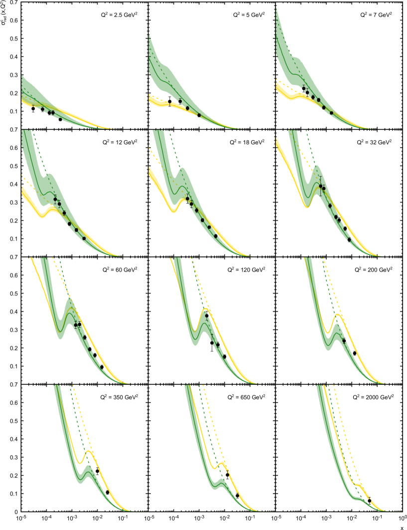
Figure 1: The reduced charm cross sections $\sigma^{c\bar{c}}_{\rm red}(x,Q^{2})$ as a function of $x$ calculated at different $Q^{2}$ values. The predictions obtained with analytical TMD gluon density in a proton and CCFM-evolved one are shown by the solid green and yellow curves, respectively. The shaded bands correspond to the scale uncertainties of our calculations. The dashed curves represent the contributions from SF $F_{2}^{c}(x,Q^{2})$, as it is described in the text. The experimental data are from H1 and ZEUS[1].

Our numerical results for reduced cross sections $\sigma^{c\overline{c}}_{\rm red}$ and $\sigma^{b\overline{b}}_{\rm red}$ are shown in Figs. 1 and 2, respectively, in comparison with the latest H1 and ZEUS data [1]. The shaded bands represent the theoretical uncertainties of our calculations. We find that the $k_{T}$-factorization predictions obtained using derived analytical expressions for TMD gluon density in a proton are in perfect agreement with the HERA data in a wide region of $x$ and $Q^{2}$ within the theoretical and experimental uncertainties, both in normalization and shape. These results tend to slightly overshoot the JH’2013 set 2 predictions in the region of small $x$ and especially at low $Q^{2}$. At larger $Q^{2}$ and/or moderate or large $x\geq 10^{-2}$ the CCFM-evolved gluon density tends to overestimate the HERA data, that could be due to the determination of corresponding input parameters at small $x$ only (see[70]). To estimate the scale uncertainties of our calculations, the standard variations (by a factor of $2$) in default renormalization and factorization scales, which were set to be equal to $\mu_{R}^{2}=4m_{Q}^{2}+Q^{2}$ and $\mu_{F}^{2}=Q^{2}$, respectively, were introduced. To show the contribution of the longitudinal structure functions $F_{L}^{c}(x,Q^{2})$ and $F_{L}^{b}(x,Q^{2})$, we present also in Figs. 1 and 2 the results for $F_{2}^{c}(x,Q^{2})$ and $F_{2}^{b}(x,Q^{2})$ as dotted curves. The difference between the estimated $\sigma^{Q\bar{Q}}_{\rm red}$ and $F_{2}^{Q}(x,Q^{2})$ is coming from the contribution of the longitudinal SFs $F_{L}^{Q}(x,Q^{2})$, as it can been clearly seen from (46). So, our calculations show that these contributions are rather important at low $x$.

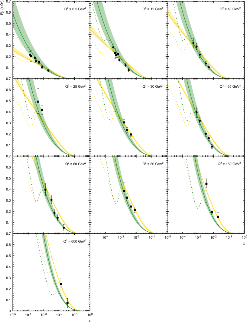
Figure 3: The charm contribution to the proton structure function $F_{2}(x,Q^{2})$ as a function of $x$ calculated at different $Q^{2}$ values. Notation of all curves is the same as in Fig. 1. The experimental data are from ZEUS[37] and H1[38].

To show the difference between $\sigma^{Q\bar{Q}}_{\rm red}$ and $F_{2}^{Q}(x,Q^{2})$ more clearly, in Figs. 3 and 4 we present our results for SFs $F_{2}^{c}(x,Q^{2})$ and $F_{2}^{b}(x,Q^{2})$ in comparison with the latest ZEUS[37] and H1[38, 39] data. Our corresponding predictions for the reduced cross sections $\sigma^{c\overline{c}}_{\rm red}$ and $\sigma^{b\overline{b}}_{\rm red}$ are presented here as dotted curves. One can see again that the results obtained with analytically evaluated TMD gluon density are in good agreement with the latest HERA data for both structure functions $F_{2}^{c}(x,Q^{2})$ and $F_{2}^{b}(x,Q^{2})$ in a wide region of $x$ and $Q^{2}$. The CCFM-evolved gluon JH’2013 set 2 provides a bit worse description of the HERA data, although these results are rather close to the measurements. We find that the discrepancy between two considered approaches tends to be more clearly pronounced at large $Q^{2}$.

4.2 Ratio $\overline{R}^{Q}(x,Q^{2})$

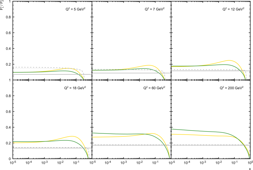
Figure 5: The charm and beauty contribution to the ratio $\hat{R}^{c}(x,Q^{2})$ as a function of $x$ calculated at different $Q^{2}$ values. Notation of green and yellow solid curves is the same as in Fig. 1. The collinear results for $\hat{R}^{c}_{\rm LO}(x,Q^{2})$, $\hat{R}^{c}_{\rm NLO}(x,Q^{2})$ and $\hat{R}^{c}_{\rm NNLO}(x,Q^{2})$ are represented by solid, dashed and dotted gray curves, respectively.

Following the results of[52] and using our coefficient functions obtained in Section 2 and TMD gluon density presented in Section 3, now we can produce predictions for the ratio $\overline{R}^{Q}(x,Q^{2})$ according to (47). Results of our calculations for $\overline{R}^{c}(x,Q^{2})$ are presented in Fig. 5, where we plot this ratio as a function of $x$ in a wide $Q^{2}$ range. As earlier, we have applied two TMD gluon densities in a proton discussed above.

Our calculations leads to more or less flat (independent on $x$) behaviour of $\overline{R}^{c}(x,Q^{2})$ with $\overline{R}^{c}\sim 0.1$ at low $Q^{2}\sim 5$ GeV² and $\overline{R}^{c}\sim 0.3-0.4$ at higher $Q^{2}\sim 200$ GeV² values. The results obtained with our TMD gluon and CCFM-evolved one are in a good agreement to each other. The difference between them is visible at very large $Q^{2}$ only. Moreover, the obtained predictions are in good agreement with ones[52], which were based in-turn on rather old representations for TMD gluon density (see[73] and more recent[3]).

As a next point of our study, we would like to compare the results for the ratio $\overline{R}^{c}(x,Q^{2})$, obtained in $k_{T}$-factorization with the one $\hat{R}^{c}(x,Q^{2})$ (see A4), where the ratio $\hat{R}^{c}(x,Q^{2})$ was obtained in the conventional (collinear) QCD factorization at first three orders of perturbation theory (see Appendix A) represented by the solid, dashed and dotted grey curves in Fig. 5. To evaluate the latter, we have used the LO DAS parton densities presented in Section 3.2. Note that the results for this ratio, obtained using the power-like behaviour $x^{-\Delta}$ of the collinear PDFs, can be found in[74]. Our calculations show that the $k_{T}$-factorization predictions rather close to the results obtained beyond LO of collinear perturbation theory. This is in complete agreement with the usual statement about the property of $k_{T}$-factorization, which resums the main part of higher order pQCD contributions at small $x$. Indeed, the LO results obtained in the collinear perturbation theory lead to too small values for the ratio $\hat{R}^{c}(x,Q^{2})$. However, the $Q^{2}$-dependence of the ratio $\hat{R}^{c}(x,Q^{2})$ in the NLO and NNLO results are noticebly different from the corresponding $Q^{2}$-dependence evaluated with the TMD gluons. In fact, in the $k_{T}$-factorization approach the ratio $\overline{R}^{c}(x,Q^{2})$ grows fastly when $Q^{2}$ increased whereas in collinear perturbation theory the ratio $\hat{R}^{c}(x,Q^{2})$ grows slowly.

Of course, the observed difference between the predicted $\overline{R}^{c}(x,Q^{2})$ and $\hat{R}^{c}(x,Q^{2})$ ratios at moderate and large $Q^{2}$ is unclear and needs an explanation, especially because there are no experimental data for the SF $F_{L}^{c}(x,Q^{2})$ and, accordingly, for the ratio $\overline{R}^{c}(x,Q^{2})$. Indeed, the $k_{T}$-factorization with the estimated $\overline{R}^{c}(x,Q^{2})$ leads to good agreement between experimental data and theoretical predictions for both reduced cross sections $\sigma^{c\overline{c}}_{\rm red}$ and SF $F_{2}^{c}(x,Q^{2})$, as one can see in Figs. 1 and 3. From another side, the experimental data for both $\sigma^{c\overline{c}}_{\rm red}$ and $F_{2}^{c}(x,Q^{2})$ are in good agreement with the corresponding theoretical predictions obtained in the framework of collinear approach[1, 37, 38, 39] (see also section 2.5 in the recent review[46]). However, we would like to note that there is a quite similar situation between the exclusive reduced cross section $\sigma_{\rm red}(x,Q^{2})$ and $F_{2}(x,Q^{2})$: experimental data for both of these observables are in good agreement with the corresponding theoretical predictions (see[75] and discussions therein), where the calculated SF $F_{L}(x,Q^{2})$ is known to be very sensitive to low $x$ resummation (see, for example, Section 9.3 in the recent review[46]). But, apart of $F_{L}^{c}(x,Q^{2})$, the SF $F_{L}(x,Q^{2})$ is measured at the HERA (see[76] and references therein). Therefore, it seems that in order to understand the observed difference between the predictions for $\overline{R}^{c}(x,Q^{2})$ and $\hat{R}^{c}(x,Q^{2})$ ratios at large $Q^{2}$ one have to investigate first the SF $F_{L}(x,Q^{2})$ using the same approaches, that is out of our present consideration. We plan to perform such investigation in forthcoming study and then, having experience in the latter, return to the study its heavy quark parts and, correspondingly, the ratio $\overline{R}^{c}(x,Q^{2})$.

5 Conclusions

We have studied the heavy quark production processes with using the transverse momentum dependent gluon distribution function in a proton obtained recently[29] using the Kimber-Martin-Ryskin prescription from the Bessel-inspired behavior of parton densities at small Bjorken $x$ values. The Bessel-like behavior of parton densities at small Bjorken $x$ was obtained[30, 31, 32, 33] in-turn in the case of the flat initial conditions for DGLAP evolution equations in the double scaling QCD approximation. To construct the TMD parton distributions we implemented[29] the different treatments of kinematical constraint, reflecting the angular and strong ordering conditions and discussed the relations between the differential and integral formulation of the KMR approach. Additionally, we have tested the TMD gluon density in a proton obtained from the numerical solution of the CCFM evolution equation, which smoothly interpolates between the small-$x$ BFKL dynamics and large-$x$ DGLAP ones.

We have considered the (reduced) cross sections $\sigma^{Q\bar{Q}}_{\rm red}$ (where $Q=c,b$) and charm and beauty contributions to the deep inelastic proton SFs $F_{2}(x,Q^{2})$ and $F_{L}(x,Q^{2})$. To show an importanse of the longitudinal structure function $F_{L}^{c}(x,Q^{2})$ and $F_{L}^{b}(x,Q^{2})$, we compare the results for $\sigma^{c\overline{c}}_{\rm red}$ and $\sigma^{b\overline{b}}_{\rm red}$ with the SFs and $F_{2}^{c}(x,Q^{2})$ and $F_{2}^{b}(x,Q^{2})$. We achieved a good agreement between the HERA experimental data for these observables and our theoretical predictions and demostrated the importance of the contributions of $F_{L}^{c}(x,Q^{2})$ and $F_{L}^{b}(x,Q^{2})$ at small $x$. Concerning the ratio of the proton SFs, namely, $\overline{R}^{c}(x,Q^{2})=F_{L}^{c}(x,Q^{2})/F_{2}^{c}(x,Q^{2})$, we show that the results of $k_{T}$-factorization calculations are similar to the ones obtained beyond LO of collinear perturbation theory. This effect is clearly visible for $Q^{2}\leq 12$ GeV². However, starting with $Q^{2}\geq 12$ GeV², the $k_{T}$-factorization leads to larger values for the ratio $\hat{R}^{c}(x,Q^{2})$, that needs an additional investigations.

As we discussed already in Section 4.2, as the next step, we plan to study the longitudinal structure function $F_{L}(x,Q^{2})$ and compare our future results with the previous ones [77, 61] and [59, 78, 79], obtained in the framework of $k_{T}$-factorization and collinear perturbation theory, respectively. This study is important in itself and will provide some kind of clue for solving the problem of differences in the predictions for the ratio $\overline{R}^{c}(x,Q^{2})$ obtained in the framework of $k_{T}$-factorization approach and conventional (collinear) QCD factorization (see Section 4.2).

Moreover, we plan to extend the present analysis beyond the LO approximation. We will obtain the results for the NLO TMD parton densities using the corresponding NLO results [30, 31, 32] for the standard PDFs in the generalized DAS approach. We will accept also the results for the NLO matrix elements (see [80, 27] and references and discussions therein). Such results are seems to be extremely important for future experiments, in particular, for experiments at the Electron-Ion Collider (EIC) and Electron-Ion Collider in China (EiCC) (see[83, 84] and discussions and references therein). So, at the EIC, an essential low $x$ (up to $x\sim 10^{-4}$) region is expected to be probed, thus providing us with new and precise data for DIS SFs, especially data for longitudinal SF $F_{L}(x,Q^{2})$. The EiCC could provide a new information on the light and sea quark density in a proton, that is, of course, important to produce and update the theoretical high-order predictions for $F_{L}(x,Q^{2})$. Moreover, EIC and EiCC measurements could be important to distinguish between the different non-collinear QCD evolution scenarios widely discussed at present (see, for example, review [2]).

Appendix A. Collinear approach

It is easily to obtain the following results in the collinear generalized DAS approach (see [81, 82]):

$$\hat{F}_{k}^{Q}(x,Q^{2})=C_{k,g}(x,Q^{2},m^{2}_{Q})\,\otimes f_{g}(x,Q^{2}),$$ (A1)

where the SFs, obtained in the generalized DAS approach, were marked as $\hat{F}_{k}^{Q}(x,Q^{2})$. Here $\otimes$ is the Mellin convolution:

$$C_{k,g}(x,Q^{2},m^{2}_{f})\,\otimes f_{g}(x,Q^{2}) = \int_{x/x_{2}}^{1}\,\frac{dy}{y}\,C_{k,g}(x/y,Q^{2},m^{2}_{f})\,f_{g}(y,Q^{2})$$ (A2)

$$= \int_{x}^{x_{2}}\,\frac{dy}{y}\,C_{k,g}(y,Q^{2},m^{2}_{f})\,f_{g}(x/y,Q^{2}),$$

where

$$x_{2}=x_{1}(b=0)~{}=~{}\frac{1}{1+4a_{Q}}.\,$$ (A3)

It can be represented as

$$\hat{R}^{Q}(x,Q^{2})=\frac{\hat{F}_{L}^{Q}(x,Q^{2})}{\hat{F}_{2}^{Q}(x,Q^{2})}=\frac{C_{L,g}(x,Q^{2},m^{2}_{Q})\,\otimes f_{g}(x,Q^{2})}{C_{2,g}(x,Q^{2},m^{2}_{Q})\,\otimes f_{g}(x,Q^{2})}\,,$$ (A4)

where $f_{g}(x,Q^{2})$ is given in (31). In fact, the ratio $\hat{R}^{Q}(x,Q^{2})$ depends slowly on non-perturbative input $f_{g}(x,Q^{2})$, which contribute to the both numerator and denominator of the ratio $\hat{R}^{Q}(x,Q^{2})$.

Using the results of $k_{T}$-factorization and BFKL approach[5, 85] (see also[86, 87]), the results for the high energy limit of collinear coefficient functions of the heavy quark production process in all orders of perturbation theory were obtained. Thus, using the results[85], below we give formulas for the high energy asymptotics of collinear coefficient functions of the heavy quark production process in the first three orders of the perturbation theory.

LO

Taking the LO Wilson coefficient (20), results (24) and (25) for on-shell coefficient functions and the PDFs considered in the section 3.2, we have for the ratio $\hat{R}^{Q}_{\rm LO}(x,Q^{2})$:

$$\hat{R}^{Q}_{\rm LO}(x,Q^{2})=\frac{B^{(0)}_{L,g}(x,Q^{2},m^{2}_{Q})\,\otimes f_{g}(x,Q^{2})}{B^{(0)}_{2,g}(x,Q^{2},m^{2}_{Q})\,\otimes f_{g}(x,Q^{2})}\,,$$ (A5)

where the dependence of gluon density $f_{g}(x,Q^{2})$ should be rather week. In fact, there is no $x$-dependence at all (see Fig. 5), which is associated with the property of the Mellin convolution (A2) in the low $x$ region (see Appendix B).

NLO

Through NLO, we have

$$C_{k,g}(x)~{}=~{}e_{Q}^{2}a_{s}(\mu^{2})\,\bigl{[}B^{(0)}_{k,g}(x,a)+a_{s}(\mu^{2})\,B^{(1)}_{k,g}(x,a)\bigr{]}\,.$$ (A6)

The NLO coefficient functions $B^{(1)}_{k,g}(x,a)$ of photon-gluon fusion subprocess are rather lengthy and not published in print; they are only available as computer codes[88]. Following [81, 82], it is sufficient to work in the high energy regime, defined by $x\ll 1$, where they assume the compact form[86, 86, 87]:

$$B_{k,g}^{(1)}(x,a)=\beta\bigl{[}R_{k,g}^{(1)}(1,a)+4C_{A}B_{k,g}^{(0)}(1,a)L_{\mu}\bigr{]}\,,~{}~{}L_{\mu}=\ln\frac{M^{2}}{\mu^{2}}\,,M^{2}=4m^{2},\,$$ (A7)

with

$$R_{2,g}^{(1)}(1,a)~{}=~{}\frac{8}{9}C_{A}[5+(13-10a)J(a)+6(1-a)I(a)],~{}~{}$$

$$R_{L,g}^{(1)}(1,a)~{}=~{}-\frac{16}{9}C_{A}x_{2}\bigl{\{}1-12a-[3+4a(1-6a)]J(a)+12a(1+3a)I(a)\bigr{\}}$$ (A8)

and

$$B_{2,g}^{(0)}(1,a) = \frac{2}{3}\,[1+2(1-a)J(a)],$$

$$B_{L,g}^{(0)}(1,a) = \frac{4}{3}\,x_{2}\,[1+6a-4a(1+3a)J(a)],$$ (A9)

where

$$J(a)=-\sqrt{x_{2}}\ln t,\qquad t=\frac{1-\sqrt{x_{2}}}{1+\sqrt{x_{2}}},$$ (A10)

$$I(a)=-\sqrt{x_{2}}\left[\zeta(2)+\frac{1}{2}\ln^{2}t-\ln(ax_{2})\ln t+2\mathop{\mathrm{Li}}\nolimits_{2}(-t)\right]$$ (A11)

with

$$\mathop{\mathrm{Li}}\nolimits_{2}(x)=-\int_{0}^{1}\,\frac{dy}{y}\,\ln(1-xy)$$ (A12)

being the dilogarithmic function. We would like to note that $B_{k,g}^{(0)}(1,a)$ are the first moments of the LO Wilson coefficients $B_{k,g}^{(0)}(x,a)$ (see (24) and (25)):

$$B_{k,g}^{(0)}(n,a)=\int_{0}^{x_{2}}dx\,x^{n-2}B_{k,g}^{(0)}(x,a)\,.$$ (A13)

So, at the NLO we have for the ratio $\hat{R}^{Q}(x,Q^{2})$:

$$\hat{R}^{Q}_{\rm NLO}(x,Q^{2})=\frac{\bigl{[}B^{(0)}_{L,g}(x,a)+a_{s}(\mu^{2})\,B^{(1)}_{L,g}(x,a)\bigr{]}\,\otimes f_{g}(x,Q^{2})}{\bigl{[}B^{(0)}_{2,g}(x,a)+a_{s}(\mu^{2})\,B^{(1)}_{2,g}(x,a)\bigr{]}\,\otimes f_{g}(x,Q^{2})}\,,$$ (A14)

where the LO gluon density $f_{g}(x,Q^{2})$ given by (31) is used because its contribution to the ratio $\hat{R}^{Q}_{\rm NLO}(x,Q^{2})$ is strongly suppressed (see Appendix B).

NNLO

Following to the results [87], we have for the coefficient function:

$$C_{k,g}(x)~{}=~{}e_{Q}^{2}a_{s}(\mu^{2})\,\bigl{[}B^{(0)}_{k,g}(x,a)+a_{s}(\mu^{2})\,B^{(1)}_{k,g}(x,a)+a^{2}_{s}(\mu^{2})\,B^{(2)}_{k,g}(x,a)\bigr{]}\,,$$ (A15)

where in the high energy regime the coeffcicient $B^{(2)}_{k,g}(x,a)$ has the compact form:

$$B_{k,g}^{(2)}(x,a)=\beta\,\ln(1/x)\,\bigl{[}R_{k,g}^{(2)}(1,a)+4C_{A}R_{k,g}^{(1)}(1,a)L_{\mu}+8C_{A}^{2}B_{k,g}^{(0)}(1,a)L^{2}_{\mu}\bigr{]}+O(x^{0})\,,$$ (A16)

with

$$R_{2,g}^{(2)}(1,a)~{}=~{}\frac{32}{27}C_{A}^{2}\,[46+(71-92a)J(a)+3(13-10a)I(a)-9(1-a)K(a)],~{}~{}$$

$$R_{L,g}^{(1)}(1,a)~{}=~{}\frac{64}{27}C_{A}^{2}x_{2}\bigl{\{}34+240a-[3+136a+480a^{2}]J(a)+3[3+4a(1-6a)]I(a)$$

$$\hskip 56.9055pt+18a(1+3a)K(a)\bigr{\}}\,,$$ (A17)

where $J(a)$ and $I(a)$ are defined by (A10) and (A11), respectively, and

$$K(a) = -\sqrt{x_{2}}\biggl{[}4\Bigl{(}\zeta(3)+\mathop{\mathrm{Li}}\nolimits_{3}(-t)-\mathop{\mathrm{Li}}\nolimits_{2}(-t)\ln t-2S_{1,2}(-t)\Bigr{)}+2\ln(ax_{2})$$ (A18)

$$\times\Bigl{(}\zeta(2)+2\mathop{\mathrm{Li}}\nolimits_{2}(-t)\Bigr{)}-\frac{1}{3}\ln^{3}t-\ln^{2}(ax_{2})\ln t+\ln(ax_{2})\ln^{2}t\biggr{]},$$

where $t$ is given in (A10) and

$$\mathop{\mathrm{Li}}\nolimits_{3}(x)=\int_{0}^{1}\,\frac{dy}{y}\,\ln(y)\,\ln(1-xy),~{}~{}S_{1,2}(x)=\frac{1}{2}\,\int_{0}^{1}\,\frac{dy}{y}\,\ln^{2}(1-xy),~{}$$ (A19)

are the trilogarithmic function $\mathop{\mathrm{Li}}\nolimits_{3}(x)$ and Nilsen Polylogarithm $S_{1,2}(x)$ (see[89]). The results for $K(a)$ in the form of harmonic Polylogarithms[90] can be found in[87].

So, at the NNLO we have for the ratio $\hat{R}^{Q}(x,Q^{2})$:

$$\hat{R}^{Q}_{\rm NNLO}(x,Q^{2})=\frac{\bigl{[}B^{(0)}_{L,g}(x,a)+a_{s}(\mu^{2})\,B^{(1)}_{L,g}(x,a)+a^{2}_{s}(\mu^{2})\,B^{(2)}_{L,g}(x,a)\bigr{]}\,\otimes f_{g}(x,Q^{2})}{\bigl{[}B^{(0)}_{2,g}(x,a)+a_{s}(\mu^{2})\,B^{(1)}_{2,g}(x,a)+a^{2}_{s}(\mu^{2})\,B^{(2)}_{2,g}(x,a)\bigr{]}\,\otimes f_{g}(x,Q^{2})}\,,$$ (A20)

where the LO gluon density $f_{g}(x,Q^{2})$ given by (31) is used because its contribution to the ratio $\hat{R}^{Q}_{\rm NNLO}(x,Q^{2})$ is strongly suppressed (see Appendix B).

Appendix B. Collinear results in DAS approach

The use of the DAS approach for the PDFs makes it possible to significantly simplify the formulas for the relation $\hat{R}^{Q}(x,Q^{2})$. We will show this below.

Taking the results (24) and (25) for on-shell coefficient functions and the PDFs considered in the section 3.2, it is easily to obtain the following LO results in the generalized DAS approach (see[81]):

$$\hat{F}^{Q}_{k}(x,Q^{2})=M_{k,g}(1,Q^{2},m^{2}_{Q})\,f_{g}(x,Q^{2}),$$ (B1)

where $M_{k,g}(1,Q^{2},m^{2})$ is the first Mellin moment ($n=1$) (see (A10)), where the Mellin moments can be defined as

$$M_{k,g}(n,Q^{2},m^{2}_{Q})=\int_{0}^{x_{2}}dx\,x^{n-2}C_{k}^{g}(x,Q^{2},m^{2}_{Q})\,,$$ (B2)

where $x_{2}$ are given by (A3). In fact, the non-perturbative input $f_{g}(x,Q^{2})$ does cancel in the $\hat{R}_{f}$ ratio and we have

$$\hat{R}^{Q}(x,Q^{2})=\frac{\hat{F}_{L}^{Q}(x,Q^{2})}{\hat{F}_{2}^{Q}(x,Q^{2})}=\frac{M_{L,g}(1,Q^{2},m_{Q}^{2})}{M_{2,g}(1,Q^{2},m_{Q}^{2})},$$ (B3)

in the case, where the moments $M_{k,g}(1,Q^{2},m_{Q}^{2})$ have no singularities at $n\to 1$.

LO

Taking the integral (B2), which becomes to be (A13) at the LO, we can obtain the results (A9), using (see[81]) the following auxiliary formulas

$$\int_{0}^{x_{2}}\,dx\,x^{m}\beta = \left\{\begin{array}[]{ll}1-2aJ(a),&\mbox{if}~{}m=0\\ \frac{x_{2}}{2}[1+6a-4a(1+3a)J(a)],&\mbox{if}~{}m=1\\ \frac{x_{2}^{2}}{3}[(1+3a)(1+10a)-6a(1+6a+10a^{2})J(a)],&\mbox{if}~{}m=2\\ \end{array}\right.,\qquad$$ (B7)

$$\int_{0}^{b}\,dx\,x^{m}\,L(\beta) = \left\{\begin{array}[]{ll}J(a),&\mbox{if}~{}m=0\\ -\frac{x_{2}}{2}[1-(1+2a)J(a)],&\mbox{if}~{}m=1\\ -\frac{x_{2}^{2}}{6}[3(1+2a)-2(1+4a+6a^{2})J(a)],&\mbox{if}~{}m=2\end{array}\right.\,$$ (B11)

So, at LO the small-$x$ approximation formula (A5) thus reads

$$\hat{R}^{Q}_{\rm LO}(x,Q^{2})=2x_{2}\frac{1+6a_{Q}-4a_{Q}(1+3a_{Q})J(a_{Q})}{1+2(1-a_{Q})J(a_{Q})}\,,$$ (B12)

which is $x$-independent, that is in full agreement with the numerical evaluation of the $\overline{R}^{Q}_{\rm LO}(x,Q^{2})$ in (A5).

NLO

At NLO, the coefficient function $C^{g}_{k}(x)$ has the form (A6) with the NLO coefficients $B^{(1)}_{k,g}(x,a)$ given by (A7) and (A8). Its moments $M_{k,g}(n,Q^{2},\mu^{2})$ exhibit the corresponding structure

$$M_{k,g}(n,Q^{2},\mu^{2})=e_{Q}^{2}a_{s}(\mu^{2})\,\bigl{[}B^{(0)}_{k,g}(n,a)+a_{s}(\mu^{2})\,B^{(1)}_{k,g}(n,a)\bigr{]}\,.$$ (B13)

The Mellin transforms of $B_{k,g}^{(1)}(x,a)$ exhibit singularities in the limit $n\to 1$, which lead to modifications in (B1). As was shown[91], the terms involving $1/\delta$ at $n=1+\delta\to 1$ (which correspond to singularities of the Mellin moments $M_{k,g}(n)$ (see (B2)) at $n\to 1$) depend on the exact form of the asymptotic low-$x$ behavior encoded in $f_{g}(x,\mu^{2})$. Using the results for $f_{g}(x,\mu^{2})$ from (31), we obtain the modification is simple modification (see[81] and discussions therein)

$$\frac{1}{\delta}\to\frac{1}{\tilde{\delta}_{\pm}},~{}~{}\frac{1}{\tilde{\delta}_{+}(x)}\approx\frac{1}{\rho_{g}(x,\mu)}\,,~{}~{}\frac{1}{\tilde{\delta}_{-}(x)}\approx\ln\frac{1}{x},$$ (B14)

where $\rho_{g}(x,\mu)$ are given by (38).

Because the ratio $f_{g}^{-}(x,Q^{2})/f_{g}^{+}(x,Q^{2})$ is rather small at the $Q^{2}$ values considered, the expression (B1) is modified to become

$$\hat{F}_{k}^{Q}(x,Q^{2})\approx\tilde{M}_{k,g}(1,\mu^{2},a)xf_{g}(x,\mu^{2}),$$ (B15)

where $\tilde{M}_{k,g}(1,\mu^{2})$ is obtained from $M_{k,g}(n,\mu^{2})$ by taking the limit $n\to 1$ and replacing $1/(n-1)\to 1/\tilde{\delta}_{+}$ in $B_{k,g}^{(1)}(n,a)$. Consequently, one needs to substitute only

$$B_{k,g}^{(1)}(1,a)\to\tilde{B}_{k,g}^{(1)}(1,a)$$ (B16)

in the NLO part of (B22), i.e.

$$\tilde{M}_{k,g}(1,Q^{2},\mu^{2})=e_{Q}^{2}a_{s}(\mu^{2})\,\bigl{[}B^{(0)}_{k,g}(1,a)+a_{s}(\mu^{2})\,\tilde{B}^{(1)}_{k,g}(1,a)\bigr{]}.$$ (B17)

Using the identity

$$\frac{1}{I_{0}(\sigma(\hat{x}))}\int^{1}_{\hat{x}}\frac{dy}{y}\beta\left(\frac{x}{y}\right)I_{0}(\sigma(y))\approx\frac{1}{\tilde{\delta}_{+}(\hat{x})}+\phi_{1}(a)\equiv\frac{1}{\hat{\delta}_{+}},~{}~{}\hat{x}=\frac{x}{x_{2}}\,,$$ (B18)

where

$$\phi_{1}(a)=-\ln(ax_{2})-\hat{J}(a),~{}~{}\hat{J}(a)=\frac{J(a)}{x_{2}}\,,$$ (B19)

we find the Mellin transform (B2) of (A7) to be

$$\tilde{B}_{k,g}^{(1)}(1,a)\approx\frac{1}{\hat{\delta}_{+}}\,\bigl{[}R_{k,g}^{(1)}(1,a)+4C_{a}B_{k,g}^{(0)}(1,a)L_{\mu}\bigr{]}\,,$$ (B20)

with $R_{k,g}^{(1)}(1,a)$ and $B_{k,g}^{(0)}(1,a)$ are given in (A8) and (A9), respectively.

So, at the NLO we have for the ratio $\hat{R}^{Q}(x,Q^{2})$:

$$\hat{R}^{Q}_{\rm NLO}(x,Q^{2})\approx\ \frac{\tilde{M}_{L,g}(1,Q^{2},m_{f}^{2})}{\tilde{M}_{2,g}(1,Q^{2},m_{f}^{2})}=\frac{B_{L,g}^{(0)}(1,a)+a_{s}(\mu^{2})\,\tilde{B}_{L,g}^{(1)}(1,a)}{B_{2,g}^{(0)}(1,a)+a_{s}(\mu^{2})\,\tilde{B}_{2,g}^{(1)}(1,a)}\,,$$ (B21)

where the ratio has some $x$-dependence coming from the corresponding $x$-dependence of $\hat{\delta}_{+}$ in (B18). The $x$-dependence is in rather good agreement with the numerical results in (A20).

NNLO

At NNLO, the coefficient function $C^{g}_{k}(x)$ has the form (A15) with the NNLO coefficients $B^{(2)}_{k,g}(x,a)$ given in Eqs. (A16) and (A17). Its moment $M_{2,g}(n,Q^{2},\mu^{2})$ exhibits the corresponding structure

$$M_{k,g}(n,Q^{2},\mu^{2})=e_{Q}^{2}a_{s}(\mu^{2})\,\bigl{[}B^{(0)}_{k,g}(n,a)+a_{s}(\mu^{2})\,B^{(1)}_{k,g}(n,a)+a^{2}_{s}(\mu^{2})\,B^{(2)}_{k,g}(n,a)\bigr{]}\,.$$ (B22)

The Mellin transforms of $B_{k,g}^{(2)}(x,a)$ exhibit singularities in the limit $n\to 1$, which has the form

$$\frac{1}{(n-1)^{2}}\to\frac{1}{\tilde{\delta}^{2}_{++}}=\frac{1}{\rho^{2}(x,\mu)}\,\frac{I_{2}(\sigma)}{I_{0}(\sigma)}\,,$$ (B23)

where all definitions can be found in (32) and (33). So, by analogy with the NLO case, we have

$$\tilde{M}_{k,g}(1,Q^{2},\mu^{2})=e_{Q}^{2}a_{s}(\mu^{2})\,\bigl{[}B^{(0)}_{k,g}(1,a)+a_{s}(\mu^{2})\,\tilde{B}^{(1)}_{k,g}(1,a)+a^{2}_{s}(\mu^{2})\,\tilde{B}^{(2)}_{k,g}(1,a)\bigr{]}\,.$$ (B24)

Using the identity

$$\frac{1}{I_{0}(\sigma(\hat{x}))}\int^{1}_{\hat{x}}\frac{dy}{y}\beta\left(\frac{x}{y}\right)\,\ln\left(\frac{y}{x}\right)I_{0}(\sigma(y))\approx\frac{1}{\tilde{\delta}^{2}_{++}(\hat{x})}\equiv\frac{1}{\hat{\delta}^{2}_{++}},~{}~{}\hat{x}=\frac{x}{x_{1}}\,,$$ (B25)

we find the Mellin transform (B2) of (A7) to be

$$\tilde{B}_{k,g}^{(2)}(1,a)\approx\frac{1}{\hat{\delta}^{2}_{++}}\,\bigl{[}R_{k,g}^{(2)}(1,a)+4C_{A}R_{k,g}^{(1)}(1,a)L_{\mu}+8C_{A}^{2}B_{k,g}^{(0)}(1,a)L^{2}_{\mu}\bigr{]}$$ (B26)

with $R_{k,g}^{(2)}(1,a)$, $R_{k,g}^{(1)}(1,a)$ and $B_{k,g}^{(0)}(1,a)$ are given in (A17), (A8) and (A9), respectively.

So, we have for the ratio $\hat{R}^{Q}(x,Q^{2})$:

$$\hat{R}^{Q}_{\rm NNLO}(x,Q^{2})\approx\ \frac{B_{L,g}^{(0)}(1,a)+\,a_{s}(\mu^{2})\,\tilde{B}_{L,g}^{(1)}(1,a)+\,a^{2}_{s}(\mu^{2})\,\tilde{B}_{L,g}^{(2)}(1,a)}{B_{2,g}^{(0)}(1,a)+\,a_{s}(\mu^{2})\,\tilde{B}_{2,g}^{(1)}(1,a)+\,a^{2}_{s}(\mu^{2})\,\tilde{B}_{2,g}^{(2)}(1,a)}\,,$$ (B27)

where the ratio has some $x$-dependence coming from the corresponding $x$-dependence of $\hat{\delta}_{++}$ in (B25). The $x$-dependence is in rather good agreement with the numerical results in (A20).

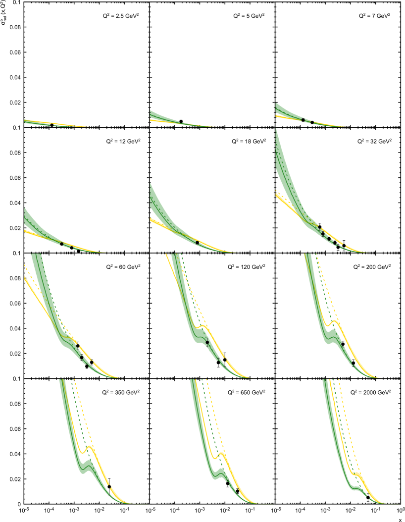
Figure 2: The reduced beauty cross sections $\sigma^{b\bar{b}}_{\rm red}(x,Q^{2})$ as a function of $x$ calculated at different $Q^{2}$ values. Notation of all curves is the same as in Fig. 1. The experimental data are from H1 and ZEUS[1].

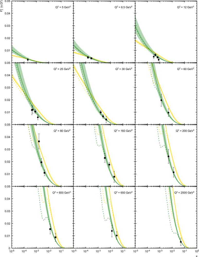
Figure 4: The beauty contribution to the proton structure function $F_{2}(x,Q^{2})$ as a function of $x$ calculated at different $Q^{2}$ values. Notation of all curves is the same as in Fig. 1. The experimental data are from ZEUS[37] and H1[39].

References

- [1] H. Abramowicz et al. [H1 and ZEUS Collaborations], Eur. Phys. J. C 78, no. 6, 473 (2018)
- [2] R. Angeles-Martinez et al., Acta Phys. Polon. B 46, 2501 (2015).
- [3] N. A. Abdulov et al., “TMDlib2 and TMDplotter: a platform for 3D hadron structure studies,” arXiv:2103.09741 [hep-ph].
- [4] J.C. Collins, D.E. Soper, G.F. Sterman, Nucl. Phys. B 223, 381 (1983), Nucl. Phys. B 250, 199 (1985).
- [5] S. Catani, M. Ciafaloni, F. Hautmann, Nucl. Phys. B 366, 135 (1991).
- [6] J.C. Collins, R.K. Ellis, Nucl. Phys. B 360, 3 (1991).
-
[7]
L.V. Gribov, E.M. Levin, M.G. Ryskin, Phys. Rep. 100, 1 (1983);
E.M. Levin, M.G. Ryskin, Yu.M. Shabelsky, A.G. Shuvaev, Sov. J. Nucl. Phys. 53, 657 (1991). -
[8]
E.A. Kuraev, L.N. Lipatov, V.S. Fadin, Sov. Phys. JETP 44, 443 (1976);
Sov. Phys. JETP 45, 199 (1977);
I.I. Balitsky, L.N. Lipatov, Sov. J. Nucl. Phys. 28, 822 (1978). -
[9]
M. Ciafaloni, Nucl. Phys. B 296, 49 (1988);
S. Catani, F. Fiorani, G. Marchesini, Phys. Lett. B 234, 339 (1990); Nucl. Phys. B 336, 18 (1990);
G. Marchesini, Nucl. Phys. B 445, 49 (1995). - [10] A.V. Lipatov, M.A. Malyshev, H. Jung, Phys. Rev. D 100, 034028 (2019).
- [11] S.P. Baranov, A.V. Lipatov, Phys.Rev. D 100, no.11, 114021 (2019).
- [12] S.P. Baranov, A.V. Lipatov, Phys. Lett. B 785, 338 (2018).
- [13] S.P. Baranov, H. Jung, A.V. Lipatov, M.A. Malyshev, Eur. Phys. J. C 77, 772 (2017).
- [14] N.A. Abdulov, A.V. Lipatov, M.A. Malyshev, Phys. Rev. D 97, 054017 (2018).
- [15] A.V. Lipatov, M.A. Malyshev, N.P. Zotov, Phys. Lett. B 735, 79 (2014).
- [16] R. Islam, M. Kumar, V.S. Rawoot, Eur. Phys. J. C 79, 181 (2019).
- [17] A. Szczurek, M. Luszczak, R. Maciula, Phys. Rev. D 90, 094023 (2014).
- [18] H. Jung, M. Krämer, A.V. Lipatov, N.P. Zotov, Phys. Rev. D 85, 034035 (2012).
- [19] H. Jung, M. Krämer, A.V. Lipatov, N.P. Zotov, JHEP 1101, 085 (2011).
- [20] S. Dooling, F. Hautmann, H. Jung, Phys. Lett. B 736, 293 (2014).
-
[21]
V.N. Gribov and L.N. Lipatov, Sov.J. Nucl. Phys. 15, 438 (1972);
L.N. Lipatov, Sov. J. Nucl. Phys. 20, 94 (1975);
G. Altarelli, G. Parisi, Nucl. Phys. B 126, 298 (1977);
Yu.L. Dokshitzer, Sov. Phys. JETP 46, 641 (1977). - [22] F. Hautmann, H. Jung, A. Lelek, V. Radescu, R. Zlebcik, Phys. Lett. B 772, 446 (2017); JHEP 1801, 070 (2018).
-
[23]
M.A. Kimber, A.D. Martin, M.G. Ryskin, Phys. Rev. D 63, 114027 (2001);
G. Watt, A.D. Martin, M.G. Ryskin, Eur. Phys. J. C 31, 73 (2003). - [24] A.D. Martin, M.G. Ryskin, G. Watt, Eur. Phys. J. C 66, 163 (2010).
- [25] R. Abdul Khalek et al. [NNPDF Collaboration], Eur. Phys. J. C (2019) 79:838
- [26] T. J. Hou et al., “Progress in the CTEQ-TEA NNLO global QCD analysis,” arXiv:1908.11394 [hep-ph]; Phys. Rev. D 103 (2021) no.1, 014013
- [27] R. Maciula, A. Szczurek, Phys. Rev. D 100, 054001 (2019).
- [28] A.V. Lipatov, M.A. Malyshev, H. Jung, Phys. Rev. D 101, no. 3, 034022 (2020).
- [29] A. V. Kotikov, A. V. Lipatov, B. G. Shaikhatdenov and P. Zhang, JHEP 2002, 028 (2020)
- [30] G. Cvetic, A.Yu. Illarionov, B.A. Kniehl, A.V. Kotikov, Phys. Lett. B 679, 350 (2009).
- [31] A.V. Kotikov, G. Parente, Nucl. Phys. B 549, 242 (1999).
- [32] A.Yu. Illarionov, A.V. Kotikov, G. Parente, Phys. Part. Nucl. 39, 307 (2008).
- [33] L. Mankiewicz, A. Saalfeld, T. Weigl, Phys. Lett. B 393, 175 (1997).
- [34] A. De Rújula, S.L. Glashow, H.D. Politzer, S.B. Treiman, F. Wilczek, A. Zee, Phys. Rev. D 10, 1649 (1974).
- [35] A.V. Lipatov, M.A. Malyshev, S.P. Baranov, Eur. Phys. J. C 80, 330 (2020).
- [36] K. Golec-Biernat, A.M. Stasto, Phys. Lett. B 781, 633 (2018).
- [37] ZEUS Collaboration, JHEP 1409, 127 (2014).
- [38] H1 Collaboration, Eur. Phys. J. C 71, 1769 (2011); Eur. Phys. J. C 72, 2252 (2012).
- [39] H1 Collaboration, Eur. Phys. J. C 65, 89 (2010).
- [40] C. Adloff et al. [H1 Collaboration], Z. Phys. C 72 (1996) 593; Nucl. Phys. B 545 (1999) 21.
- [41] J. Breitweg et al. [ZEUS Collaboration], Phys. Lett. B 407 (1997) 402; Eur. Phys. J. C 12 (2000) 35
- [42] J. J. Aubert et al. [European Muon Collaboration], Nucl. Phys. B 213 (1983) 31; Phys. Lett. 94B (1980) 96; Phys. Lett. 110B (1982) 73.
- [43] R. Aaij et al. [LHCb Collaboration], Nucl. Phys. B 871 (2013) 1; JHEP 1706 (2017) 147; JHEP 1603 (2016) 159 Erratum: [JHEP 1609 (2016) 013] Erratum: [JHEP 1705 (2017) 074]
- [44] A. M. Cooper-Sarkar, R. C. E. Devenish and A. De Roeck, Int. J. Mod. Phys. A 13 (1998) 3385
- [45] O. Zenaiev, Eur. Phys. J. C 77 (2017) no.3, 151
- [46] J. Gao, L. Harland-Lang and J. Rojo, Phys. Rept. 742 (2018) 1
-
[47]
M. Cacciari, M. L. Mangano and P. Nason,
Eur. Phys. J. C 75 (2015) no.12, 610;
O. Zenaiev et al. [PROSA Collaboration], Eur. Phys. J. C 75 (2015) no.8, 396;
R. Gauld and J. Rojo, Phys. Rev. Lett. 118 (2017) no.7, 072001. -
[48]
A. Cooper-Sarkar, P. Mertsch and S. Sarkar,
JHEP 1108 (2011) 042;
R. Fiore et al., Phys. Rev. D 68 (2003) 093010; Phys. Rev. D 71 (2005) 033002; Phys. Rev. D 73 (2006) 053012;
A. Y. Illarionov, B. A. Kniehl and A. V. Kotikov, Phys. Rev. Lett. 106 (2011) 231802 -
[49]
R. Gauld, J. Rojo, L. Rottoli, S. Sarkar and J. Talbert,
JHEP 1602 (2016) 130;
M. V. Garzelli et al. [PROSA Collaboration], JHEP 1705 (2017) 004 -
[50]
J. L. Abelleira Fernandez et al. [LHeC Study Group],
J. Phys. G 39 (2012) 075001;
“On the Relation of the LHeC and the LHC,”
arXiv:1211.5102 [hep-ex];
N. Armesto [LHeC Study Group], J. Phys. Conf. Ser. 422 (2013) 012030. - [51] M. L. Mangano et al., CERN Yellow Rep. (2017) no.3, 1 [arXiv:1607.01831 [hep-ph]].
- [52] A.V. Kotikov, A.V. Lipatov, G. Parente, N.P. Zotov, Eur. Phys. J. C 26, 51 (2002).
-
[53]
E. Witten,
Nucl. Phys. B104 (1976) 445;
M. Gluck and E. Reya, Phys. Lett. B83 (1979) 98;
F.M. Steffens, W. Melnitchouk, and A.W. Thomas, Eur.Phys.J. C11 (1999) 673. - [54] A.J. Buras, Rev. Mod. Phys. 52, 199 (1980).
- [55] A.V. Kotikov, B.G. Shaikhatdenov, Phys. Part. Nucl. 48, 829 (2017); Phys. Atom. Nucl. 78, 525 (2015); Phys. Part. Nucl. 44, 543 (2013).
- [56] B. Badelek, J. Kwiecinski, A. Stasto, Z. Phys. C 74, 297 (1997).
-
[57]
D.V. Shirkov, I.L. Solovtsov, Phys. Rev. Lett. 79, 1209 (1997);
I.L. Solovtsov, D.V. Shirkov, Theor. Math. Phys. 120, 1220 (1999). -
[58]
G. Cvetic, C. Valenzuela, Braz. J. Phys. 38, 371 (2008);
A.P. Bakulev, Phys. Part. Nucl. 40, 715 (2009);
N.G. Stefanis, Phys. Part. Nucl. 44, 494 (2013). - [59] A.V. Kotikov, Phys. Lett. B 338, 349 (1994)
-
[60]
Yu.L. Dokshitzer, D.V. Shirkov, Z. Phys. C 67, 449 (1995);
S.J. Brodsky, V.S. Fadin, V.T. Kim, L.N. Lipatov, G.B. Pivovarov, JETP Lett. 70, 155 (1999);
Small- Collaboration, Eur. Phys. J. C 25, 77 (2002). - [61] A. V. Kotikov, A. V. Lipatov and N. P. Zotov, J. Exp. Theor. Phys. 101, 811 (2005)
- [62] A.V. Kotikov, B.G. Shaikhatdenov, P. Zhang, Phys. Part. Nucl. Lett. 16 no.4, 311 (2019) [ arXiv:1811.05615 [hep-ph]].
- [63] A.V. Kotikov, B.G. Shaikhatdenov, P. Zhang, Phys. Rev. D 96, 114002 (2017).
-
[64]
C. Lopez, F.J. Yndurain, Nucl. Phys. B 171, 231 (1980);
Nucl. Phys. B 183, 157 (1981);
A.Yu. Illarionov, A.V. Kotikov, S.S. Parzycki, D.V. Peshekhonov, Phys. Rev. D 83, 034014 (2011). -
[65]
V.A. Matveev, R.M. Muradian, A.N. Tavkhelidze, Lett. Nuovo Cim. 7, 719 (1973);
S.J. Brodsky, G.R. Farrar, Phys. Rev. Lett. 31, 1153 (1973);
S.J. Brodsky, J.R. Ellis, E.Gardi, M. Karliner, M.A. Samuel, Phys. Rev. D 56, 6980 (1997). -
[66]
P. Jimenez-Delgado, E. Reya, Phys. Rev. D 89, 074049 (2014);
S. Alekhin, J. Blümlein, S. Moch, R. Placakyte, Phys. Rev. D 96, 014011 (2017). -
[67]
V.G. Krivokhizhin, A.V. Kotikov, Phys. Atom. Nucl. 68, 1873 (2005);
Phys. Part. Nucl. 40, 1059 (2009);
B.G. Shaikhatdenov, A.V. Kotikov, V.G. Krivokhizhin, G. Parente, Phys. Rev. D 81, 034008 (2010);
A.V. Kotikov, V.G. Krivokhizhin, B.G. Shaikhatdenov, Phys. Atom. Nucl. 75, 507 (2012); J. Phys. G 42, no. 9, 095004 (2015); Phys. Atom. Nucl. 81, 244 (2018). - [68] CMS Collaboration, JHEP 1204, 084 (2012).
- [69] ATLAS Collaboration, Eur. Phys. J. C 71, 1846 (2011).
- [70] F. Hautmann, H. Jung, Nucl. Phys. B 883, 1 (2014).
- [71] L.A. Harland-Lang, A.D. Martin, P. Motylinski, R.S. Thorne, Eur. Phys. J. C 75, 435 (2015).
- [72] PDG Collaboration, Rev. D 98, 030001 (2018).
-
[73]
J. Blumlein, “On the -dependent gluon density in hadrons and in the photon, in ’95 QCD and high-energy hadronic
interactions. Proceedings, 30th Rencontres de Moriond, MoriondParticle Physics Meetings, Hadronic Session, Le Arcs, France, March 19-25, 1995, pp.191–197. 1995. Also in preprint hep-ph/9506446;
M. G. Ryskin and Y. M. Shabelski, Z. Phys. C 61 (1994) 517; Z. Phys. C 66 (1995) 151. -
[74]
N. Y. Ivanov and B. A. Kniehl,
Eur. Phys. J. C 59, 647 (2009);
G. R. Boroun, “Importance of the heavy-quarks longitudinal structure function measurements at future circular collider energies,” arXiv:2101.11829 [hep-ph]. - [75] H. Abramowicz et al. [H1 and ZEUS Collaborations], Eur. Phys. J. C 75 (2015) no.12, 580; F. D. Aaron et al. [H1 and ZEUS Collaborations], JHEP 1001 (2010) 109
- [76] V. Andreev et al. [H1 Collaboration], Eur. Phys. J. C 74 (2014) no.4, 2814
- [77] A.V. Kotikov, A.V. Lipatov, N.P. Zotov, Eur. Phys. J. C 27, 219 (2003).
-
[78]
A. V. Kotikov,
J. Exp. Theor. Phys. 80, 979 (1995);
A. V. Kotikov and G. Parente, Mod. Phys. Lett. A 12, 963 (1997); J. Exp. Theor. Phys. 85, 17 (1997) - [79] L. P. Kaptari, A. V. Kotikov, N. Y. Chernikova and P. Zhang, Phys. Rev. D 99, no. 9, 096019 (2019); JETP Lett. 109, no. 5, 281 (2019)
-
[80]
A. van Hameren, “A note on QED gauge invariance of off-shell amplitudes”,
arXiv:1902.01791 [hep-ph];
M. Nefedov, V. Saleev, Mod. Phys. Lett. A 32, 1750207 (2017);
F. Caporale, F. G. Celiberto, G. Chachamis, D. Gordo Gomez, A. Sabio Vera, AIP Conf. Proc. 1819, 060009 (2017). - [81] A.Yu. Illarionov, B.A. Kniehl, A.V. Kotikov, Phys. Lett. B 663, 66 (2008); “Heavy-quark contributions to the ratio F(L)/F(2) at low values of the Bjorken variable x,” Proceedings, Helmholz International Summer School on Heavy Quark Physics, p.243-252. 2008. Also in preprint arXiv:0812.4943 [hep-ph].
- [82] A.Yu. Illarionov, A.V. Kotikov, Phys. Atom. Nucl. 75, 1234 (2012).
- [83] A. Accardi et al., Eur. Phys. J. A 52 (2016) no.9, 268
- [84] D. P. Anderle et al., “Electron-Ion Collider in China,” arXiv:2102.09222 [nucl-ex].
- [85] S. Catani, Z. Phys. C 75 (1997) 665.
- [86] S. Catani, M. Ciafaloni and F. Hautmann, Preprint CERN-Th.6398/92, in Proceeding of the Workshop on Physics at HERA (Hamburg, 1991), Vol. 2., p. 690; S. Catani and F. Hautmann, Nucl. Phys. B 427 (1994) 475; S. Riemersma, J. Smith and W. L. van Neerven, Phys. Lett. B 347 (1995) 143
- [87] H. Kawamura, N. A. Lo Presti, S. Moch and A. Vogt, Nucl. Phys. B 864, 399 (2012)
- [88] E. Laenen, S. Riemersma, J. Smith and W. L. van Neerven, Nucl. Phys. B 392 (1993) 162, 229.
- [89] A. Devoto and D. W. Duke, Riv. Nuovo Cim. 7N6, 1 (1984).
- [90] E. Remiddi and J. A. M. Vermaseren, Int. J. Mod. Phys. A 15 (2000) 725
- [91] A.V. Kotikov, Phys. Part. Nucl. 38, 1 (2007) 1; [Erratum-ibid. 38 (2007) 828].