Barrow Holographic Dark Energy in non-flat Universe

Abstract

We construct Barrow holographic dark energy in the case of non-flat universe. In particular, considering closed and open spatial geometry we extract the differential equations that determine the evolution of the dark-energy density parameter, and we provide the analytical expression for the corresponding dark energy equation-of-state parameter. We show that the scenario can describe the thermal history of the universe, with the sequence of matter and dark energy epochs. Comparing to the flat case, where the phantom regime is obtained for relative large Barrow exponents, the incorporation of positive curvature leads the universe into the phantom regime for significantly smaller values. Additionally, in the case of negative curvature we find a reversed behavior, namely for increased Barrow exponent we acquire algebraically higher dark-energy equation-of-state parameters. Furthermore, we confront the scenario with Hubble parameter measurements and supernova type Ia data. Hence, the incorporation of slightly non-flat spatial geometry to Barrow holographic dark energy improves the phenomenology while keeping the new Barrow exponent to smaller values.

I Introduction

According to the general consensus of modern cosmology, supported by a huge amount of cosmological observations, the Universe experienced accelerated expansion at both early and late times. In order to provide an explanation one has two main directions to follow. The first path is to introduce new forms of matter, such as the inflaton Olive:1989nu ; Bartolo:2004if or the dark energy concept Copeland:2006wr ; Cai:2009zp , while maintaining general relativity as the gravitational theory. The second path, is to construct extended and modified gravitational theories, which in general give rise to the extra degree(s) of freedom capable of triggering acceleration, but still possess general relativity as a particular limit CANTATA:2021ktz ; Capozziello:2011et ; Cai:2015emx .

Nevertheless, holographic dark energy Li:2004rb ; Wang:2016och and holographic inflation Nojiri:2019kkp is an interesting alternative for the quantitative description of acceleration, that strictly speaking does not fall in the above two solution ways. It arises from the cosmological application of the holographic principle tHooft:1993dmi ; Bousso:2002ju ; Fischler:1998st , and the induced connection between the Ultraviolet cutoff of a quantum field theory with the largest length Cohen:1998zx , which finally results to a vacuum energy of holographic origin. Holographic dark energy leads to interesting cosmological phenomenology Li:2004rb ; Wang:2016och ; Horvat:2004vn ; Pavon:2005yx ; Wang:2005jx ; Nojiri:2005pu ; Kim:2005at ; Wang:2005ph ; Setare:2008pc ; Setare:2008hm , it is in agreement with observations Zhang:2005hs ; Li:2009bn ; Feng:2007wn ; Zhang:2009un ; JWLee:2007JCAP ; Lu:2009iv ; Micheletti:2009jy ; DAgostino:2019wko ; Sadri:2019qxt ; Molavi:2019mlh , and it has been extended to various versions Gong:2004fq ; Saridakis:2007cy ; Setare:2007we ; Cai:2007us ; Setare:2008bb ; Saridakis:2007ns ; Saridakis:2007wx ; Jamil:2009sq ; Gong:2009dc ; Suwa:2009gm ; BouhmadiLopez:2011xi ; Chimento:2011pk ; Malekjani:2012bw ; Chimento:2013se ; Khurshudyan:2014axa ; Landim:2015hqa ; Pasqua:2015bfz ; Jawad:2016tne ; Pourhassan:2017cba ; Nojiri:2017opc ; Saridakis:2017rdo ; Saridakis:2018unr ; Aditya:2019bbk ; Geng:2019shx ; Waheed:2020cxw ; Saha:2021ngs ; Saleem:2021iju .

We should comment here that holographic dark energy models may face the causality problem Kim:2013epl . In particular, the present accelerated expansion requires the future event horizon to be the universe boundary Li:2004rb , which in turn depends on the future evolution of the scale factor and thus it might violate causality Cai:2007us . Nevertheless, a number of possibilities have been explored to address this problem. It has been shown that suitable modifications of the gravitational sector in the scalar-tensor theories of gravity Xu:2009EPJ or various modified holographic models such as Agegraphic dark energy Cai:2007us , Ricci dark energy Gao:2009prd ; Zhang:2009un etc, can alleviate the problem through suitable alternative choices of the universe horizon. Additionally, there have been other approaches in which the causality problem can been resolved, by separating out the “future-dependent” part from the evolution equation Kim:2013epl , since this part carries the information of the causality violation which can be fixed by properly choosing the initial conditions.

In order to apply the holographic principle and construct holographic dark energy one uses the black hole entropy expression, and thus one can obtain various versions of the theory through the use of different entropies. Recently Barrow proposed a new black hole entropy relation that arises from the incorporation of quantum-gravitational effects which may introduce intricate, fractal features on the black-hole area, namely Barrow:2020tzx

$$S_{B}=\left(\frac{A}{A_{0}}\right)^{1+\frac{\Delta}{2}},$$ (1)

with $A$ the standard horizon area ($A_{0}$ is the Planck area). The new exponent $\Delta$ lies in the range $0\leq\Delta\leq 1$, with $\Delta=0$ corresponding to the standard smooth structure (in which case Barrow entropy gives back the standard Bekenstein-Hawking ones), and with $\Delta=1$ corresponding to the most intricate structure. Hence, application of this extended entropy relation as the basis of holographic dark energy gives rise to Barrow holographic dark energy Saridakis:2020zol which is able to offer improved phenomenology comparing to the standard scenarios of holographic dark energy Saridakis:2020zol ; Anagnostopoulos:2020ctz ; Abreu:2020cyv ; Saridakis:2020lrg ; Mamon:2020spa ; Abreu:2020rrh ; Abreu:2020dyu ; Dabrowski:2020atl ; Abreu:2020wbz ; Barrow:2020kug ; Srivastava:2020cyk ; Das:2020rmg ; Sharma:2020ylh ; Pradhan:2021cbj ; Sheykhi:2021fwh ; Bhardwaj:2021chg ; Chakraborty:2021uzp .

On the other hand, recently there is a reheated debate on whether the spatial curvature of the universe is zero or not. In particular, there are arguments that if one considers the combined analysis of Cosmic Microwave Background (CMB) anisotropy power spectra of the Planck Collaboration with the luminosity distance data, then a non-flat universe is favored at 99% confidence level DiValentino:2020hov . Additionally the enhanced lensing amplitude in the CMB power spectrum seems to suggest that the curvature index $k$ may be positive Akrami:2018vks .

Having these in mind, in the present work we are interested in constructing and investigating Barrow Holographic dark energy in a non-flat universe. The paper is organized as follows: In Section II we present the basic equations for Barrow Holographic dark energy in both closed and open Friedmann-Robertson-Walker (FRW) metric. In Section III we proceed to a detailed investigation of the cosmological behavior, focusing on the dark energy density and equation-of-state parameters. In section IV we present the observational constraints on various parameters of the model and finally, we summarize our results in Section V.

II Barrow holographic dark energy in non-flat geometry

In this section we desire to construct holographic dark energy in the case of non-zero spatial curvature. In particular, we consider a non-flat FRW line element of the form

$$ds^{2}=-\;dt^{2}+a^{2}(t)\left[\frac{dr^{2}}{1-kr^{2}}+r^{2}d\Omega^{2}\right],$$ (2)

where $a(t)$ is the scale factor and $k=+1,0,-1$ corresponds to closed, flat and open spatial curvature respectively.

In general, by applying Barrow entropy (1) in the holographic framework, one obtains a holographic dark energy density of the form Saridakis:2020zol

$$\rho_{DE}=CL^{\Delta-2},$$ (3)

with $L$ the holographic horizon length and $C$ a parameter with dimensions $[L]^{-2-\Delta}$. Note that in the case where Barrow entropy becomes the usual Bekenstein-Hawking one, namely for $\Delta=0$, expression (3) gives the standard holographic dark energy $\rho_{DE}=CL^{-2}$ with $C=3{c^{2}}{M_{p}}^{2}$, where $c^{2}$ is the standard parameter of order one that is present in all holographic dark energy models Li:2004rb ; Wang:2016och and $M_{p}$ the Planck mass.

We consider that the universe is filled with the above holographic dark energy, as well as the matter sector. The Friedmann equations are written as

$$3H^{2}+3\frac{k}{a^{2}}={\rho}_{m}+{\rho}_{DE}$$ (4)

$$2\dot{H}+3H^{2}+\frac{k}{a^{2}}=-p_{DE},$$ (5)

with $H\equiv\dot{a}/a$ the Hubble parameter, and where $\rho_{m}$ is the energy density corresponding to the matter perfect fluid assumed to be dust, while $p_{DE}$ represents the pressure of the Barrow holographic dark energy. The two components are separately conserved, namely they obey

$${\dot{\rho}}_{m}+3H\rho_{m}=0$$ (6)

$${\dot{\rho}}_{DE}+3H\left(1+w_{DE}\right)\rho_{DE}=0,$$ (7)

where we have introduced the dark-energy effective equation-of-state parameter as $w_{DE}\equiv\frac{p_{DE}}{\rho_{DE}}$. Finally, it proves convenient to introduce the density parameters through $\Omega_{m}\equiv\frac{\rho_{m}}{3M_{p}^{2}H^{2}}$, $\Omega_{DE}\equiv\frac{\rho_{DE}}{3M_{p}^{2}H^{2}}$ and $\Omega_{k}\equiv\frac{k}{a^{2}H^{2}}$.

The last step that we need to perform is to suitably define the largest length $L$ of the theory, namely the holographic horizon that enters in the definition of holographic dark energy. Although there are many possible choices, in the case of flat spatial geometry the most common one is to use the future event horizon Li:2004rb , namely

$$R_{h}\equiv a\int_{t}^{\infty}\frac{dt}{a}=a\int_{a}^{\infty}\frac{da}{Ha^{2}}$$ (8)

However, if one desires to extend holographic dark energy in a non-flat universe, the above length should be suitably extended Huang:2004ai ; Setare:2006wh . Hence, in the case of Barrow holographic dark energy this recipe should be followed too (note that in Dixit:2021phd it was tried to apply Barrow holographic dark energy in a non-flat universe but with $L$ being the Hubble horizon, a choice that is known to be not correct Li:2004rb ; Hsu:2004ri since it cannot lead to acceleration). Since the corresponding extension is slightly different for closed and open cases, in the following subsections we examine them separately.

II.1 Positive spatial curvature

Let us start with the case of closed universe ($k=+1$). The horizon length $L$ is given by $L=ar(t)$, where $r(t)$ is determined through Huang:2004ai ; Setare:2006wh

$$\int_{0}^{r(t)}\frac{dr^{\prime}}{\sqrt{1-k{r^{\prime}}^{2}}}=\frac{R_{h}}{a}.$$ (9)

Thus, one obtains

$$r(t)=\frac{1}{\sqrt{k}}\sin y,$$ (10)

where

$$y=\sqrt{k}\frac{R_{h}}{a}=\sqrt{k}\int_{x}^{\infty}\frac{dx}{aH},$$ (11)

with $x=\ln a$. Hence, inserting $L=ar(t)$ into (3) we obtain the holographic dark energy density

$$\rho_{DE}=Ca^{\Delta-2}\left(\frac{1}{\sqrt{k}}\sin y\right)^{\Delta-2}.$$ (12)

In the following it proves convenient to use the values of the density parameters at present, denoted by the subscript “0”:

$$\Omega_{m}=\frac{\Omega_{m0}H_{0}^{2}}{a^{3}H^{2}},\ \ \ \ \Omega_{k}=\frac{\Omega_{k0}H_{0}^{2}}{a^{2}H^{2}},$$ (13)

which in turn gives

$$\frac{\Omega_{k}}{\Omega_{m}}=a\gamma,$$ (14)

with $\gamma\equiv\frac{\Omega_{k0}}{\Omega_{m0}}$.

Inserting (12) into (4), and using the density parameters, we obtain

$$\frac{1}{aH}=\frac{1}{\sqrt{{\Omega_{m}}_{0}}H_{0}}\ \left(\frac{1-\Omega_{DE}}{a^{-1}-\gamma}\right)^{\frac{1}{2}},$$ (15)

while further insertion into (11),(10) leads to

$$L=\frac{a}{\sqrt{k}}\ \sin\left[\sqrt{k}\int_{x}^{\infty}\frac{dx}{H_{0}\sqrt{\Omega_{m0}}}\left(\frac{1-\Omega_{DE}}{a^{-1}-\gamma}\right)^{\frac{1}{2}}\right].$$ (16)

On the other hand, substituting (3) into (4), and using the density parameters, gives

$$L=\left[\frac{(1-\Omega_{DE})}{\Omega_{DE}}\frac{C}{3M_{p}^{2}H_{0}^{2}\Omega_{m0}}\frac{a^{2}}{(a^{-1}-\gamma)}\right]^{\frac{1}{2-\Delta}}\;.$$ (17)

Equating (16) and (17) one obtains the equation

$$\begin{split}\frac{a}{\sqrt{k}}\ \sin\left[\sqrt{k}\int_{x}^{\infty}\frac{dx}{H_{0}\sqrt{\Omega_{m0}}}\left(\frac{1-\Omega_{DE}}{a^{-1}-\gamma}\right)^{\frac{1}{2}}\right]\\ =\left[\frac{(1-\Omega_{DE})}{\Omega_{DE}}\frac{C}{3M_{p}^{2}H_{0}^{2}\Omega_{m0}}\frac{a^{2}}{(a^{-1}-\gamma)}\right]^{\frac{1}{2-\Delta}}.\end{split}$$ (18)

Differentiating equation(18) with respect to $x=\ln a$ we acquire

$$\begin{split}\frac{\Omega_{DE}^{\prime}}{\Omega_{DE}(1-\Omega_{DE})}=\Delta+1+\gamma e^{x}(1-\gamma e^{x})^{-1}+\left[Q\cos y\right.\\ \left.(\Omega_{DE})^{\frac{1}{2-\Delta}}(1-\Omega_{DE})^{\frac{\Delta}{2(\Delta-2)}}e^{\frac{3\Delta x}{2(\Delta-2)}}(1-\gamma e^{x})^{\frac{\Delta}{2(2-\Delta)}}\right],\end{split}$$ (19)

with

$$Q\equiv(2-\Delta)\left(\frac{C}{3M_{p}^{2}}\right)^{\frac{1}{\Delta-2}}\left(H_{0}\sqrt{\Omega_{m0}}\right)^{\frac{\Delta}{2-\Delta}},$$

and with primes denoting derivatives with respect to $x=\ln a$ .

Differential equation (19) determines the evolution of Barrow holographic dark energy for dust matter in a closed universe. In the case where $\gamma=0$ (i.e. $\Omega_{k}=0$) it coincides with Barrow holographic dark energy in flat universe Saridakis:2020zol . Additionally, in the case where $\Delta=0$ it coincides with the usual holographic dark energy in a closed universe Huang:2004ai ; Setare:2006wh . Finally, for $\gamma=0$ and $\Delta=0$ it gives back the standard holographic dark energy in a flat universe, namely $\Omega_{DE}^{\prime}|_{{}_{\Delta=0}}=\Omega_{DE}(1-\Omega_{DE})\left(1+2\sqrt{\frac{3M_{p}^{2}\Omega_{DE}}{{C}}}\right)$, which accepts an analytic solution (in implicit form) Li:2004rb .

We close this subsection by extracting the expression for the dark-energy equation-of-state parameter $w_{DE}$. Differentiating (12), using (11),(10), and inserting into (7), we easily obtain

$$\begin{split}w_{DE}=-\left(\frac{1+\Delta}{3}\right)-\frac{Q}{3}{\left(\Omega_{DE}\right)}^{\frac{1}{2-\Delta}}\cos y\\ \left(\frac{1-\Omega_{DE}}{1-\gamma e^{x}}\right)^{\frac{\Delta}{2(\Delta-2)}}e^{\frac{3\Delta x}{2(\Delta-2)}}.\end{split}$$ (20)

As expected for the flat case $\gamma=0$, equation (20) reduces to the expression obtained in Saridakis:2020zol . Moreover, for $\Delta=0$ we acquire the expression of standard holographic dark energy in closed universe Huang:2004ai ; Setare:2006wh . Finally, setting $\gamma=0$ and $\Delta=0$ we re-obtain the equation-of-state parameter for standard holographic dark energy in flat spatial geometry Wang:2016och .

II.2 Negative spatial curvature

In the case of an open universe ($k=-1$) the horizon length $L$ is given by $L=ar(t)$, where $r(t)$ is determined through Huang:2004ai ; Setare:2006wh

$$\int_{0}^{r(t)}\frac{dr^{\prime}}{\sqrt{1+k{r^{\prime}}^{2}}}=\frac{R_{h}}{a},$$ (21)

leading to

$$r(t)=\frac{1}{\sqrt{|k|}}\sinh y,$$ (22)

where

$$y=\sqrt{|k|}\frac{R_{h}}{a}=\sqrt{|k|}\int_{x}^{\infty}\frac{dx}{aH},$$ (23)

with $x=\ln a$. Proceeding similarly to the previous subsection, we obtain

$$\begin{split}\frac{a}{\sqrt{|k|}}\ \sinh\left[\sqrt{|k|}\int_{x}^{\infty}\frac{dx}{H_{0}\sqrt{\Omega_{m0}}}\left(\frac{1-\Omega_{DE}}{a^{-1}-\gamma}\right)^{\frac{1}{2}}\right]\\ =\left[\frac{(1-\Omega_{DE})}{\Omega_{DE}}\frac{C}{3M_{p}^{2}H_{0}^{2}\Omega_{m0}}\frac{a^{2}}{(a^{-1}-\gamma)}\right]^{\frac{1}{2-\Delta}}.\end{split}$$ (24)

Differentiating equation(24) with respect to $x=\ln a$ and using equation (15) we acquire

$$\begin{split}\frac{\Omega_{DE}^{\prime}}{\Omega_{DE}(1-\Omega_{DE})}=\Delta+1+\gamma e^{x}(1-\gamma e^{x})^{-1}+\left[Q\cosh y\right.\\ \left.(\Omega_{DE})^{\frac{1}{2-\Delta}}\ (1-\Omega_{DE})^{\frac{\Delta}{2(\Delta-2)}}\ e^{\frac{3\Delta x}{2(\Delta-2)}}\ (1-\gamma e^{x})^{\frac{\Delta}{2(2-\Delta)}}\right]\end{split}$$ (25)

with

$$Q\equiv(2-\Delta)\left(\frac{C}{3M_{p}^{2}}\right)^{\frac{1}{\Delta-2}}\left(H_{0}\sqrt{\Omega_{m0}}\right)^{\frac{\Delta}{2-\Delta}}.$$

Differential equation (25) provides the evolution of Barrow holographic dark energy for dust matter in an open universe. In the case where $\gamma=0$ it coincides with Barrow holographic dark energy in flat universe Saridakis:2020zol . Furthermore, in the case where $\Delta=0$ it coincides with the usual holographic dark energy in an open universe Huang:2004ai ; Setare:2006wh . Lastly, for $\gamma=0$ and $\Delta=0$ it gives back the standard holographic dark energy in a flat universe Li:2004rb .

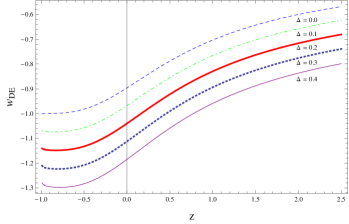
Figure 1: Upper graph: The evolution of the density parameters for matter and Barrow holographic dark energy, as a function of the redshift $z$, in the case of a closed universe ($k=+1$), for $\Delta=0.1$ and ${C}=3$, in $M_{p}^{2}=1$ units. Lower graph: The evolution of the dark-energy equation-of-state parameter $w_{DE}(z)$, for various $\Delta$ values. We have imposed $\Omega_{DE0}\approx 0.72$, $\Omega_{m0}\approx 0.27$ and $\Omega_{k0}=0.01$ at present. The vertical line marks the present time $z=0$.

We proceed to extract the expression for the dark-energy equation-of-state parameter $w_{DE}$. Differentiating (12), using (23),(22), and inserting into (7), we easily obtain

$$\begin{split}w_{DE}=-\left(\frac{1+\Delta}{3}\right)-\frac{Q}{3}{\left(\Omega_{DE}\right)}^{\frac{1}{2-\Delta}}\cosh y\\ \left(\frac{1-\Omega_{DE}}{1-\gamma e^{x}}\right)^{\frac{\Delta}{2(\Delta-2)}}e^{\frac{3\Delta x}{2(\Delta-2)}}.\end{split}$$ (26)

Similarly to the closed case, for $k=0$ equation (26) reduces to the expression for flat-universe obtained in Saridakis:2020zol , while with $\Delta=0$ we re-acquire the standard form of equation-of-state parameter for standard holographic dark energy in open universe Huang:2004ai ; Setare:2006wh . Lastly, for both $k=0$ and $\Delta=0$ we recover standard holographic dark energy in a flat universe Wang:2016och .

III Cosmological behavior

In this section we proceed to the investigation of the cosmological evolution of Barrow holographic dark energy in closed and open universe. As we mentioned above, equations (19) and (25) determine respectively the behavior of the dark-energy density parameter as a function of $x=\ln a$, for the two spatial-flatness cases. One can easily express the evolution in terms of the more convenient redshift, through $x=\ln a=-{\rm ln}(1+z)$ (setting the current scale factor value to $a_{0}=1$). We elaborate equations (19) and (25) numerically, imposing the initial conditions $\Omega_{m}(x=-\ln(1+z)=0)\equiv\Omega_{m0}$, $\Omega_{DE}(x=-\ln(1+z)=0)\equiv\Omega_{DE0}$ and $\Omega_{k}(x=-\ln(1+z)=0)\equiv\Omega_{k0}$ in agreement with recent observations Akrami:2018vks .

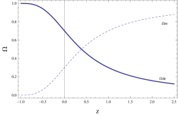
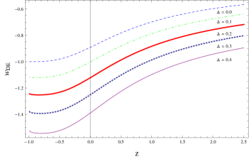
Figure 2: Upper graph: The evolution of the density parameters for matter and Barrow holographic dark energy, as a function of the redshift $z$, in the case of a closed universe ($k=+1$), for $\Delta=0.1$ and ${C}=3$, in $M_{p}^{2}=1$ units. Lower graph: The evolution of the dark-energy equation-of-state parameter $w_{DE}(z)$, for various $\Delta$ values. We have imposed $\Omega_{DE0}\approx 0.70$, $\Omega_{m0}\approx 0.299$ and $\Omega_{k0}=0.001$ at present. The vertical line marks the present time $z=0$.

In the upper graph of Fig. 1 we depict the evolution of matter and dark energy density parameters $\Omega_{m}(z)$ and $\Omega_{DE}(z)$, in the case of a closed universe, for a given value of the Barrow exponent $\Delta$. As we observe, we obtain the usual thermal history, with the sequence of matter and radiation epochs, with the transition from matter to dark energy domination happening around $z\sim 0.4$, which is in agreement with the required scenario of structure formation of the universe. Note that for more transparency we have extended the evolution up to the far future $z=-1$, where we can see that the universe results in a complete dark-energy domination as expected.

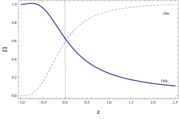
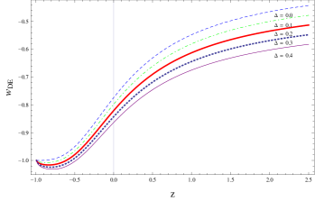
Figure 3: Upper graph: The evolution of the density parameters for matter and Barrow holographic dark energy, as a function of the redshift $z$, in the case of a closed universe ($k=+1$), for $\Delta=0.1$ and ${C}=3$, in $M_{p}^{2}=1$ units. Lower graph: The evolution of the dark-energy equation-of-state parameter $w_{DE}(z)$, for various $\Delta$ values. We have imposed $\Omega_{DE0}\approx 0.63$, $\Omega_{m0}\approx 0.27$ and $\Omega_{k0}=0.1$ at present. The vertical line marks the present time $z=0$.

In order to study in more detail the behavior of the equation-of-state parameter of Barrow holographic dark energy, and specifically to investigate how it is affected by the exponent $\Delta$ and by $\Omega_{k0}$, in the lower graph of Fig. 1 we present $w_{DE}(z)$ for the case $k=+1$, and for various $\Delta$ values. As we can see, for increasing $\Delta$ the evolution of $w_{DE}(z)$ and its current value $w_{DE}(z=0)\equiv w_{DE0}$ tend to obtain lower values. In particular, while for $\Delta=0$ the dark-energy equation-of-state parameter lies completely in the quintessence regime, for $\Delta$ deviating from 0 the universe will result in the phantom regime, and specifically for $\Delta>0.03$ the phantom-divide crossing has been realized in the past. Hence, in the case of Barrow holographic dark energy we obtain the possibility to exhibit the crossing to the phantom regime, contrary to the case of standard holographic dark energy.

We mention here that comparing to flat Barrow holographic dark energy, in which the phantom regime was obtained for relative large Barrow exponents $\Delta\geq 0.5$, the incorporation of curvature is able to drive the universe into the phantom regime for significantly smaller $\Delta$ values, which is an advantage of the scenario since realistically one expects small Barrow exponents. In order to further examine the effect of the special curvature, we repeat the whole analysis for lower as well as higher values of $\Omega_{k0}$, and the corresponding results are displayed in Figs. 2 and 3. As we observe, smaller curvature densities lead to lower $w_{DE}$ values, while the exact values of $\Omega_{m0}$ and $\Omega_{DE0}$ have insignificant effect. Additionally, we mention that in Fig. 3 we considered a non-realistically large value for $\Omega_{k0}$ in order to be able to show the tendency in more transparency. In particular, apart from the delay of the dark-energy domination (which is expected since we have imposed a lower $\Omega_{DE0}$), we observe that for all $\Delta$ values the universe remains in the quintessence regime, while in the far future, although the phantom-divide crossing is exhibited, eventually all curves tend to the de Sitter phase $w_{DE}=-1$.

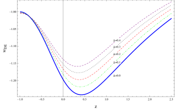
Figure 4: The evolution of the dark-energy equation-of-state parameter for Barrow holographic dark energy, as a function of the redshift $z$, in the case of an open universe ($k=-1$), for various $\Delta$ values. We have imposed $\Omega_{DE0}\approx 0.72$, $\Omega_{m0}\approx 0.29$ and $\Omega_{k0}=-0.01$ at present. The vertical line marks the present time $z=0$.

We proceed to the investigation of the negative curvature case ($k=-1$). Since the evolution of $\Omega_{m}(z)$ and $\Omega_{DE}(z)$ is similar to the upper graphs of the previous cases, with the sequence of matter and dark-energy epochs, we omit the corresponding graphs and we focus on the evolution of dark-energy equation-of-state parameter. In Fig. 4 we depict $w_{DE}(z)$ for various $\Delta$ values. Interestingly enough we now obtain a reversed behavior than in the positive-curvature case, namely the increased $\Delta$ leads to algebraically higher $w_{DE}$ values. Moreover, note that for all cases the universe is currently in the phantom regime, hence for the case of open spatial geometry the phantom regime is more favorable, contrary to the case of flat universe Saridakis:2020zol as well as to the positive curvature case analyzed above. Finally, we observe the interesting behavior that in the far future all curves converge to the de Sitter universe, with a complete dark-energy domination and $w_{DE}=-1$.

IV Observational Constraints

Figure 5: The $1\sigma$ and $2\sigma$ iso-likelihood contours for the scenario of Barrow holographic dark energy in non-flat universe, using Hubble data, in the case of negative curvature (upper panel) and positive curvature (lower panel). The black dot represents the best fit value.

In this section we proceed to the confrontation of the scenario at hand with observations, and in particular with Hubble measurements and supernova type Ia (SNIa) data.

Dataset	$k$	$\Delta~{}$	$\Omega_{k0}~{}$	$\chi_{\text{min}}/dof$
$H(z)$	Positive	$0.19$	$0.032$	$8.42$
	Negative	$0.1$	$-0.001$	$9.24$
SNIa	Positive	$0.18$	$0.01$	$9.74$
	Negative	$0.21$	$-0.15$	$8.90$
$H(z)$ $+$ SNIa	Positive	$0.2$	$0.01$	$9.14$
	Negative	$0.06$	$-0.09$	$16.23$

Table 1: Best-fit values of $\Delta$ and $\Omega_{k0}$ for Barrow holographic dark energy in the case of non-flat universe, for various datasets, alongside the corresponding $\chi_{\text{min}}/dof$ of the fit, where “dof” stands for degrees of freedom.

For the $H(z)$ data we use the 29 data points of Hubble parameter measurements zhang:2014 ; Simon:2005 ; aam:2015 in the redshift range $0.07\leq z\leq 2.34$. The corresponding $\chi^{2}$ function is defined as

$$\chi^{2}_{H}=\sum^{29}_{i=1}\frac{[{h}^{obs}(z_{i})-{h}^{th}(z_{i})]^{2}}{\sigma^{2}_{H}(z_{i})},$$ (27)

where ${h}=\frac{H(z)}{H_{0}}$ is the normalized Hubble parameter. For the SNIa dataset, we have used the Union2.1 compilation data Suzuki:2012 of 580 data points in the range $0.015\leq z\leq 1.414$. The corresponding $\chi^{2}$ reads as NesserisPRD:2005

$$\chi^{2}_{SN}=A-\frac{B^{2}}{C},$$ (28)

with $A$, $B$ and $C$ defined as

$$A=\sum^{580}_{i=1}\frac{[{\mu}^{obs}(z_{i})-{\mu}^{th}(z_{i})]^{2}}{\sigma^{2}_{i}},$$ (29)

$$B=\sum^{580}_{i=1}\frac{[{\mu}^{obs}(z_{i})-{\mu}^{th}(z_{i})]}{\sigma^{2}_{i}},$$ (30)

and

$$C=\sum^{580}_{i=1}\frac{1}{\sigma^{2}_{i}},$$ (31)

where $\mu^{obs}$ represents the observed distance modulus at a particular redshift, $\mu^{th}$ the corresponding theoretical value and $\sigma_{i}$ represents the uncertainty in the distance modulus. Hence, the total $\chi^{2}$ for these combined observational datasets is given by

$$\chi^{2}_{total}=\chi^{2}_{SN}+\chi^{2}_{H}.$$ (32)

Figure 6: The $1\sigma$ and $2\sigma$ iso-likelihood contours for the scenario of Barrow holographic dark energy in non-flat universe, using SNIa data, in the case of negative curvature (upper panel) and positive curvature (lower panel). The black dot represents the best fit value.

In Table 1 we display the resulting best-fit values for the separated datasets, as well as for the combined analysis. Additionally, in Fig. 5 we present the $1\sigma$ and $2\sigma$ confidence contours in the $\Delta-\Omega_{k0}$ parameter space in the case of Hubble data, in Fig. 6 in the case of SNIa data, and in Fig. 7 for the combined dataset analysis.

Figure 7: The $1\sigma$ and $2\sigma$ iso-likelihood contours for the scenario of Barrow holographic dark energy in non-flat universe, for the combined $H(z)$+SNIa analysis, in the case of negative curvature (upper panel) and positive curvature (lower panel). The black dot represents the best fit value.

As we observe, in the case of negative values of $k$ the Barrow exponent $\Delta$ is constrained to smaller values, closer to standard results. Concerning $\Omega_{k0}$, we can see that although the best-fit values are small, comparatively larger values of $\Omega_{k0}$ are allowed at $1\sigma$ or $2\sigma$ confidence level. Furthermore, for a comprehensive analysis we have also handled $H_{0}$ as a free parameter, and the corresponding value comes out to be $H_{0}=69.86$ km s^-1 Mpc^-1, which is closer to the value obtained by PLANCK Collaboration. Hence, the scenario at hand might offer a way to alleviate the $H_{0}$ tension DiValentino:2020zio . Nevertheless, we mention that a full investigation of this issue would require to incorporate additionally the CMB data and perform a joint analysis (see also colgain:2021 ; Guo:2018ans ). Such a full observational analysis lies beyond the scope of this first work on the model, and it is left for a future project.

V Conclusions

In this work we constructed Barrow holographic dark energy in the case of non-flat universe. The former is a holographic dark energy that arises through the usual application of the holographic principle in a cosmological framework, however it incorporates the recently proposed Barrow entropy, instead of the standard Bekenstein-Hawking one. Considering closed and open spatial geometry we extracted the simple differential equations that determine the evolution of the dark-energy density parameter, and we provided the analytical expression for the corresponding dark energy equation-of-state parameter.

Proceeding to the detailed investigation, we showed that the scenario at hand can describe the thermal history of the universe, with the sequence of matter and dark energy epochs. Furthermore, we examined the effect of the Barrow exponent $\Delta$, as well as of the curvature density parameter at present, on the dark-energy equation-of-state parameter. As we saw, while for $\Delta=0$ the dark-energy equation-of-state parameter lies completely in the quintessence regime, for $\Delta>0.03$ the phantom-divide crossing has been realized in the past, namely Barrow holographic dark favors the phantom regime.

However, the interesting feature is that comparing to the flat case, where the phantom regime was obtained for relative large Barrow exponents $\Delta\geq 0.5$, the incorporation of positive curvature leads the universe into the phantom regime for significantly smaller $\Delta$ values. This is an advantage since one expects that only small deviations from standard entropy could actually be the case. Additionally, in the case of negative curvature we found a reversed behavior, namely for increased $\Delta$ we obtained algebraically higher $w_{DE}$ values, however for all cases the universe is currently in the phantom regime. Hence, comparing to the flat and closed universe, negative curvature favors the phantom regime more intensively. Finally, we confronted the scenario at hand with Hubble parameter measurements and supernova type Ia data, and we found that it can fit observations efficiently.

In summary, the incorporation of slightly non-flat spatial geometry to Barrow holographic dark energy improves the phenomenology comparing to the flat case while keeping the new Barrow exponent to smaller values. This is an advantage of the scenario, since in a realistic case one expects the Barrow exponent to be closer to the standard Bekenstein-Hawking value.

- (1) K. A. Olive, Phys. Rept. 190, 307 (1990).
- (2) N. Bartolo, E. Komatsu, S. Matarrese and A. Riotto, Phys. Rept. 402, 103 (2004). [arXiv:astro-ph/0406398].
- (3) E. J. Copeland, M. Sami and S. Tsujikawa, Int. J. Mod. Phys. D 15, 1753 (2006). [arXiv:hep-th/0603057].
- (4) Y. -F. Cai, E. N. Saridakis, M. R. Setare and J. -Q. Xia, Phys. Rept. 493, 1 (2010). [arXiv:0909.2776].
- (5) E. N. Saridakis et al. [CANTATA], [arXiv:2105.12582].
- (6) S. Capozziello and M. De Laurentis, Phys. Rept. 509, 167 (2011). [arXiv:1108.6266].
- (7) Y. F. Cai, S. Capozziello, M. De Laurentis and E. N. Saridakis, Rept. Prog. Phys. 79, 106901 (2016). [arXiv:1511.07586].
- (8) M. Li, Phys. Lett. B 603, 1 (2004) [arXiv:hep-th/0403127].
- (9) S. Wang, Y. Wang and M. Li, Phys. Rept. 696, 1-57 (2017) [arXiv:1612.00345].
- (10) S. Nojiri, S. D. Odintsov and E. N. Saridakis, Phys. Lett. B 797, 134829 (2019) [arXiv:1904.01345].
- (11) G. ’t Hooft, Salamfest 1993: 0284-296 [arXiv:gr-qc/9310026].
- (12) R. Bousso, Rev. Mod. Phys. 74, 825 (2002) [arXiv:hep-th/0203101].
- (13) W. Fischler and L. Susskind, [arXiv:hep-th/9806039].
- (14) A. G. Cohen, D. B. Kaplan and A. E. Nelson, Phys. Rev. Lett. 82, 4971 (1999) [arXiv:hep-th/9803132].
- (15) R. Horvat, Phys. Rev. D 70, 087301 (2004) [arXiv:astro-ph/0404204].
- (16) D. Pavon and W. Zimdahl, Phys. Lett. B 628, 206 (2005) [arXiv:gr-qc/0505020].
- (17) B. Wang, Y. g. Gong and E. Abdalla, Phys. Lett. B 624, 141 (2005) [arXiv:hep-th/0506069].
- (18) S. Nojiri and S. D. Odintsov, Gen. Rel. Grav. 38, 1285 (2006) [arXiv:hep-th/0506212].
- (19) H. Kim, H. W. Lee and Y. S. Myung, Phys. Lett. B 632, 605 (2006) [arXiv:gr-qc/0509040].
- (20) B. Wang, C. Y. Lin and E. Abdalla, Phys. Lett. B 637, 357 (2006) [arXiv:hep-th/0509107].
- (21) M. R. Setare and E. N. Saridakis, Phys. Lett. B 671, 331 (2009) [arXiv:0810.0645].
- (22) M. R. Setare and E. N. Saridakis, Phys. Lett. B 670, 1 (2008) [arXiv:0810.3296].
- (23) X. Zhang and F. Q. Wu, Phys. Rev. D 72, 043524 (2005) [arXiv:astro-ph/0506310].
- (24) M. Li, X. D. Li, S. Wang and X. Zhang, JCAP 0906, 036 (2009) [arXiv:0904.0928].
- (25) C. Feng, B. Wang, Y. Gong and R. K. Su, JCAP 0709, 005 (2007) [arXiv:0706.4033].
- (26) X. Zhang, Phys. Rev. D 79, 103509 (2009) [arXiv:0901.2262].
- (27) J. W. Lee, J. Lee, H. C. Kim, JCAP 0708, 005 (2007) [arXiv:hep-th/0701199].
- (28) J. Lu, E. N. Saridakis, M. R. Setare and L. Xu, JCAP 1003, 031 (2010) [arXiv:0912.0923].
- (29) S. M. R. Micheletti, JCAP 1005, 009 (2010) [arXiv:0912.3992].
- (30) R. D’Agostino, Phys. Rev. D 99, no.10, 103524 (2019) [arXiv:1903.03836].
- (31) E. Sadri, Eur. Phys. J. C 79, no.9, 762 (2019) [arXiv:1905.11210].
- (32) Z. Molavi and A. Khodam-Mohammadi, Eur. Phys. J. Plus 134, no.6, 254 (2019) [arXiv:1906.05668].
- (33) Y. G. Gong, Phys. Rev. D 70, 064029 (2004) [arXiv:hep-th/0404030].
- (34) E. N. Saridakis, Phys. Lett. B 660, 138 (2008) [arXiv:0712.2228].
- (35) M. R. Setare and E. C. Vagenas, Int. J. Mod. Phys. D 18, 147 (2009) [arXiv:0704.2070].
- (36) R. G. Cai, Phys. Lett. B 657, 228 (2007) [arXiv:0707.4049].
- (37) E. N. Saridakis, JCAP 0804, 020 (2008) [arXiv:0712.2672].
- (38) E. N. Saridakis, Phys. Lett. B 661, 335 (2008) [arXiv:0712.3806].
- (39) M. R. Setare and E. C. Vagenas, Phys. Lett. B 666, 111 (2008) [arXiv:0801.4478].
- (40) M. Jamil, E. N. Saridakis and M. R. Setare, Phys. Lett. B 679, 172 (2009) [arXiv:0906.2847].
- (41) Y. Gong and T. Li, Phys. Lett. B 683, 241 (2010) [arXiv:0907.0860].
- (42) M. Suwa and T. Nihei, Phys. Rev. D 81, 023519 (2010) [arXiv:0911.4810].
- (43) M. Bouhmadi-Lopez, A. Errahmani and T. Ouali, Phys. Rev. D 84, 083508 (2011) [arXiv:1104.1181].
- (44) L. P. Chimento and M. G. Richarte, Phys. Rev. D 84, 123507 (2011) [arXiv:1107.4816].
- (45) M. Malekjani, Astrophys. Space Sci. 347, 405 (2013) [arXiv:1209.5512].
- (46) L. P. Chimento, M. Forte and M. G. Richarte, Eur. Phys. J. C 73, no.1, 2285 (2013) [arXiv:1301.2737].
- (47) M. Khurshudyan, J. Sadeghi, R. Myrzakulov, A. Pasqua and H. Farahani, Adv. High Energy Phys. 2014, 878092 (2014) [arXiv:1404.2141].
- (48) R. C. G. Landim, Int. J. Mod. Phys. D 25, no. 04, 1650050 (2016) [arXiv:1508.07248].
- (49) Eur. Phys. J. Plus 131, no. 11, 408 (2016) [arXiv:1511.00611].
- (50) A. Jawad, N. Azhar and S. Rani, Int. J. Mod. Phys. D 26, no. 04, 1750040 (2016).
- (51) B. Pourhassan, A. Bonilla, M. Faizal and E. M. C. Abreu, Phys. Dark Univ. 20, 41 (2018) [arXiv:1704.03281].
- (52) S. Nojiri and S. D. Odintsov, Eur. Phys. J. C 77, no. 8, 528 (2017) [arXiv:1703.06372].
- (53) E. N. Saridakis, Phys. Rev. D 97, no. 6, 064035 (2018) [arXiv:1707.09331].
- (54) E. N. Saridakis, K. Bamba, R. Myrzakulov and F. K. Anagnostopoulos, JCAP 12, 012 (2018) [arXiv:1806.01301].
- (55) Y. Aditya, S. Mandal, P. Sahoo and D. Reddy, Eur. Phys. J. C 79, no.12, 1020 (2019) [arXiv:1910.12456].
- (56) C. Q. Geng, Y. T. Hsu, J. R. Lu and L. Yin, Eur. Phys. J. C 80, no.1, 21 (2020) [arXiv:1911.06046].
- (57) S. Waheed, Eur. Phys. J. Plus 135, no.1, 11 (2020).
- (58) A. Saha, S. Ghose, A. Chanda and B. C. Paul, Annals Phys. 426, 168403 (2021) [arXiv:2101.04060].
- (59) R. Saleem and N. Shahnila, Phys. Dark Univ. 32, 100808 (2021).
- (60) H. Kim, J. W. Lee and J. Lee 102, 29001 (2013) [arXiv:1208.3729].
- (61) L. Xu, W. Li and J. Lu, 60, 135 (2009) [arXiv:astro-ph/0804.2925].
- (62) C. Gao, F. Q. Wu, X. Chen and Y. G. Shen, Phys. Rev. D 79, 043511 (2009) [arXiv:astro-ph/0712.1394]
- (63) J. D. Barrow, Phys. Lett. B 808, 135643 (2020) [arXiv:2004.09444].
- (64) E. N. Saridakis, Phys. Rev. D 102, no.12, 123525 (2020) [arXiv:2005.04115].
- (65) F. K. Anagnostopoulos, S. Basilakos and E. N. Saridakis, Eur. Phys. J. C 80, no.9, 826 (2020) [arXiv:2005.10302].
- (66) E. M. C. Abreu, J. A. Neto and E. M. Barboza, jr., EPL 130, no.4, 40005 (2020) [arXiv:2005.11609].
- (67) E. N. Saridakis, JCAP 07, 031 (2020) [arXiv:2006.01105].
- (68) A. A. Mamon, A. Paliathanasis and S. Saha, Eur. Phys. J. Plus 136, no.1, 134 (2021) [arXiv:2007.16020].
- (69) E. M. C. Abreu and J. Ananias Neto, Phys. Lett. B 807, 135602 (2020).
- (70) E. M. C. Abreu and J. A. Neto, Eur. Phys. J. C 80, no.8, 776 (2020)
- (71) M. P. Dabrowski and V. Salzano, Phys. Rev. D 102, no.6, 064047 (2020) [arXiv:2009.08306].
- (72) E. M. C. Abreu and J. A. Neto, Phys. Lett. B 810, 135805 (2020) [arXiv:2009.10133].
- (73) J. D. Barrow, S. Basilakos and E. N. Saridakis, Phys. Lett. B 815, 136134 (2021) [arXiv:2010.00986].
- (74) S. Srivastava and U. K. Sharma, Int. J. Geom. Meth. Mod. Phys. 18, no.01, 2150014 (2021) [arXiv:2010.09439].
- (75) B. Das and B. Pandey, [arXiv:2011.07337].
- (76) U. K. Sharma, G. Varshney and V. C. Dubey, Int. J. Mod. Phys. D 30, no.03, 2150021 (2021) [arXiv:2012.14291].
- (77) A. Pradhan, A. Dixit and V. K. Bhardwaj, Int. J. Mod. Phys. A 36, no.04, 2150030 (2021) [arXiv:2101.00176].
- (78) A. Sheykhi, [arXiv:2102.06550].
- (79) V. K. Bhardwaj, A. Dixit and A. Pradhan, [arXiv:2102.09946].
- (80) G. Chakraborty, S. Chattopadhyay, E. Güdekli and I. Radinschi, Symmetry 13, no.4, 562 (2021).
- (81) J. M. Bardeen, B. Carter and S. W. Hawking, Commun. Math. Phys. 31, 161-170 (1973).
- (82) S. Das, P. Majumdar and R. K. Bhaduri, Class. Quant. Grav. 19, 2355-2368 (2002) [arXiv:hep-th/0111001].
- (83) N. Suzuki et al., Astrophy. J., 746, 85 (2021) [arXiv:1105.3470].
- (84) S. Nesseris and L. Perivolaropoulos, [arXiv:astro-ph/0511040].
- (85) C. Zhang et al., Res. in Astron. and Astrophys., 14, 1221 (2014), [arXiv:1207.4541].
- (86) J. Simon et al., Phys. Rev. D 71, 123001 (2005), [arXiv:astro-ph/0412269].
- (87) A. A. Mamon and S. Das, Eur. Phys. J. C, 75, 244 (2015), [arXiv:1503.06280].
- (88) F. Beutler et al., Mon. Not. R. Astron. Soc. 416, 3017 (2011), [arXiv:1106.3366].
- (89) W. J. Percival et al., Mon. Not. R. Astron. Soc. 401, 2148 (2010), [arXiv:0907.1660 ].
- (90) C. Blake et al., Mon. Not. R. Astron. Soc. 418, 1707 (2011), [arXiv:1108.2635 ].
- (91) N. Jarosik et al., Astrophys. J. Suppl. 192, 14 (2011), [arXiv:1001.4744].
- (92) R. Goistri et al., JCAP, 03, 027 (2012), [arXiv:1203.3213].
- (93) E. Di Valentino, L. A. Anchordoqui, O. Akarsu, et al. Astropart. Phys. 131, 102605 (2021) [arXiv:2008.11284].
- (94) E. Di Valentino, A. Melchiorri and J. Silk, Astrophys. J. Lett. 908, no. 1, L9 (2021) [arXiv:2003.04935].
- (95) N. Aghanim et al. [Planck], Astron. Astrophys. 641, A1 (2020) [arXiv:1807.06205].
- (96) Q. G. Huang and M. Li, JCAP 0408, 013 (2004) [arXiv:astro-ph/0404229].
- (97) M. R. Setare, Phys. Lett. B 642, 1 (2006) [arXiv:hep-th/0609069].
- (98) A. Dixit, V. K. Bharadwaj and A. Pradhan, [arXiv:2103.08339].
- (99) S. D. H. Hsu, Phys. Lett. B 594, 13-16 (2004) [arXiv:hep-th/0403052].
- (100) E. Ó. Colgáin and M. M. Sheikh-Jabbari, Class.Quantum Grav. 38, 177001 (2021) [arXiv:2102.09816].
- (101) R. Y. Guo, J. F. Zhang and X. Zhang, JCAP 02, 054 (2019) arXiv:1809.02340].