Interpretation of multiple solutions in fully iterative GF2 and GW schemes using local analysis of two-particle density matrices

Abstract

Due to non-linear structure, iterative Green’s function methods can result in multiple different solutions even for simple molecular systems. In contrast to the wave-function methods, a detailed and careful analysis of such molecular solutions was not performed before. In this work, we use two-particle density matrices to investigate local spin and charge correlators that quantify the charge-resonance and covalent characters of these solutions. When applied within unrestricted orbital set, spin correlators elucidate the broken symmetry of the solutions, containing necessary information for building effective magnetic Hamiltonians. Based on GW and GF2 calculations of simple molecules and transition metal complexes, we construct Heisenberg Hamiltonians, four-spin-four-center corrections, as well as biquadratic spin–spin interactions. These Hamiltonian parametrizations are compared to prior wave-function calculations.

Iterative or self-consistent propagator methods that solve the Dyson equation are used across diverse areas such as nuclear and particle physicsRoberts:Dyson:hadronic:1994 ; Roberts:Dyson:QCD:2000 ; Koide:nuclear_dyson:1994 , electronic structure of moleculesStan06 ; Dahlen05 ; Ortiz:propagator:review:2013 , and condensed matter physicsMahan00 ; Negele:Orland:book:2018 ; Martin:Interacting_electrons:2016 . The self-consistent solution of the Dyson equation can be interpreted in the following way. A propagating particle interacts with the environment, changing it. The perturbed environment changes the effective interaction, affecting the particle propagator. Therefore, there is a feedback loop between the particle propagation and the environment that this self-consistent equation encodes.

The nonlinear equations appearing in iterative Green’s function methods may lead to multiple solutions Kozik15 ; Reining:Dyson:multiple_solutions:2017 ; Rossi:multivalue:2015 ; Berger:unphys_solutions:2015 fulfilling these equations. Some of these solutions are discarded as “unphysical” and only the remaining “physical” ones should be used to describe systems under study. Existence of multiple solutions is a fundamental problem, going beyond convergence difficulties or trapping in local minima. The space of acceptable physical solutions is large and deserves a careful analysis. In solids, the interpretations of such results is natural since they correspond to different thermodynamic phases. In molecular problems, such interpretation is more challenging because the association between these solutions and molecular excited states is not always straightforward when considering only the one-body density matrix (or natural orbital occupations). In the wave-function methods, the analysis of many-body wave functions can be done not only via one-electron orbitalsSalem:72:SOGeomDep ; ElSayedRule ; Michl:ACR:13 ; Ohrn:73:PROP ; Ortiz:99:PROP ; Oana:Dyson:07 ; Luzanov:TDM-1:76 ; Luzanov:TDM-2:79 ; HeadGordon:att_det:95 ; Martin:NTO:03 ; Luzanov:DMRev:12 ; Dreuw:ESSAImpl:14 ; Dreuw:ESSAImpl-2:14 ; Nanda:NTO:17 ; Wojtek:ImagEx:18 ; Krylov:Libwfa:18 ; Dreuw:NTOfeature:2019 ; Pavel:SOCNTOs:2019 ; Krylov:Orbitals ; Nanda:RIXSNTO:20 ; Nanda:NTO:hyperpolarizability:2021 , but also by examining the determinantal wave-function structureScholes:EET:1994 ; Toru:ASDDimers:13 ; Toru:ASD:14 or high-order density matricesGill:intracule:2003 ; Gill:intracule:2004 ; Luzanov:HP:06 ; Mazziotti:cumulant:norm:06 ; Plasser:NTOfeature:2020 . However, for one-body iterative Green’s functions such analysis was limited and could not be done to a comparable level since it requires information beyond the one-particle picture.

In this paper, we analyze GW and GF2 self-consistent solutions for a few strongly correlated systems by means of local spin and charge correlators. This approach, based on the recently derived two-particle density matricesPokhilko:tpdm:2021 , helps us to rationalize the underlying electronic structure and explain the character of the solutions obtained. In particular, it elucidates the broken-spin character of the solutions when applied to magnetic systems, establishing the interpretation ground of such calculations. Moreover, local spin and charge correlators serve as diagnostic tools for non-Heisenberg type interactions in magnetic species.

An imaginary-time Green’s function $G$ is defined as

$$G_{pq}(\tau)=-\frac{1}{Z}\operatorname{Tr}\left[e^{-(\beta-\tau)(H-\mu N)}pe^{-\tau(H-\mu N)}q^{\dagger}\right],$$ (1)

$$Z=\operatorname{Tr}\left[e^{-\beta(\hat{H}-\mu\hat{N})}\right],$$ (2)

where $\tau$ is the imaginary time, $\beta$ is the inverse temperature, $\mu$ is the chemical potential, $\hat{N}$ is the particle-number operator, and $Z$ is the grand-canonical partition function. Since the fermionic imaginary-time one-particle Green’s function is antiperiodic and the bosonic Green’s function is periodic, the corresponding frequency representations are discrete, known as Matsubara frequencies:

$$\omega_{n}=\frac{(2n+1)\pi}{\beta},$$ (3)

$$\Omega_{n}=\frac{2n\pi}{\beta},$$ (4)

where $\omega_{n}$ are fermionic Matsubara frequencies and $\Omega_{n}$ are bosonic Matsubara frequencies. The Dyson equation is written as

$$G^{-1}(i\omega_{n})=G^{-1}_{0}(i\omega_{n})-\Sigma[G](i\omega_{n}),$$ (5)

where the self-energy $\Sigma[G]$ is a functional of the one-particle Green’s function $G$ and $G_{0}$ is the Green’s function of independent electrons. The exact definition of the self-energy depends on the actual approximation employed.

GF2 is a perturbative method that includes contributions to the self-energy up to the second order in terms of bare Coulomb interactionSnijders:GF2:1990 ; Dahlen05 ; Phillips14 ; Rusakov16 ; Welden16 ; Iskakov19 . GW Hedin65 ; G0W0_Pickett84 ; G0W0_Hybertsen86 ; GW_Aryasetiawan98 ; Stan06 ; Koval14 ; scGW_Andrey09 approximates the static part of self-energy with Hartree–Fock exchange. The dynamic part of its self-energy is defined in terms of screened frequency dependent Coulomb interaction $W(\Omega_{n})$.

The self-consistently solved equations lead to the following structure of the two-particle density matrix

$$\Gamma_{\braket{pq}{rs}}=\gamma_{pr}\gamma_{qs}-\gamma_{ps}\gamma_{qr}+\Gamma^{\text{conn}}_{\braket{pq}{rs}},$$ (6)

$$\Gamma^{\text{disc}}_{\braket{pq}{rs}}=\gamma_{pr}\gamma_{qs}-\gamma_{ps}\gamma_{qr},$$ (7)

where $\Gamma$ is the two-particle density matrix, $\gamma$ is the one-particle density matrix, and $\Gamma^{\text{conn}}$ and $\Gamma^{\text{disc}}$ are the connected and disconnected parts of two-particle density matrix, respectively. The connected part is also known as the electronic cumulant of the two-particle density matrix.

The self-energy functional $\Sigma[G]$, particular for the approximation employed, determines the actual expression for the electronic cumulant. The GF2 and GW approximations lead to the following cumulants:

$$\Gamma_{\braket{p_{0}q_{0}}{r_{0}s_{0}}}^{\text{GF2}}=\frac{1}{\beta}\sum_{\omega_{n}}\sum_{t}I^{dir+ex,1}_{p_{0}q_{0}ts_{0}}(i\omega_{n})G_{tr_{0}}(i\omega_{n}),$$ (8)

$$I^{dir+ex,1}_{p_{0}q_{0}ts_{0}}(\tau)=-\sum_{uvw}\braket{tu}{vw}G_{vp_{0}}(\tau)G_{wq_{0}}(\tau)G_{s_{0}u}(-\tau),$$ (9)

$$\Gamma_{(p_{0}q_{0}|r_{0}s_{0})}^{\text{GW}}=-\frac{1}{\beta}\sum_{\Omega_{m}}\sum_{pqrs}\Pi_{r_{0}s_{0}pq}(\Omega_{m})W_{(pq|rs)}(\Omega_{m})\Pi_{rsp_{0}q_{0}}(\Omega_{m}),$$ (10)

where all the indices label spin-orbitals.

Figure 1: Possible configurations formed with 2 electrons and 2 localized orbitals $A$ and $B$. Local different-center charge and spin correlators are shown.

A statistical cumulantKubo:cumulant:1962 of two operators $\hat{X}$ and $\hat{Y}$ is defined as

$$\Pi_{XY}=\braket{\hat{X}\hat{Y}}-\braket{\hat{X}}\braket{\hat{Y}}=\braket{(\hat{X}-\braket{\hat{X}})(\hat{Y}-\braket{\hat{Y}})}=\braket{\delta\hat{X}\delta\hat{Y}}.$$ (11)

Statistical cumulants are also known as covariances. They measure the joint variability of two random variables. Covariances employ the mean value of the product of the deviations of two variables from their respective means/averages (here denoted as $\braket{\hat{X}}$ and $\braket{\hat{Y}}$). When deployed within localized orbitals, statistical cumulants of local operators give a local into the probe of electronic structure. For example, local charge cumulants have been used to define a chemical bond orderRuedenberg:chem_bond:1962 ; Jorge:bond_index:1985 ; Torre:popul:cumulants:2002 ; Bochicchio:bond_order:2003 ; Goddard:corr_chem_bond:1998 ; Luzanov:bond_indices:2005 ; Mayer:bond_order:2007 and local spin cumulants have been used for the analysis of polyradical speciesDavidson:local_spin:2001 ; Davidson:local_spin:2002 ; Davidson:MolMagnets:2002 ; Hess:local_spin:2005 ; Luzanov:SpinCorr:15 . Here the local operators are constructed from the integrals, expressed in orbitals localized note:nonorth in a certain space region. We follow the Mulliken-like partitioning, similar to Ref.Goddard:corr_chem_bond:1998 ; Bochicchio:bond_order:2003 ; Hess:local_spin:2005 , i.e. use atomic orbitals for partitioning of the system into fragments. Consequently, the local particle number and local spin operators on a fragment $A$ are defined as

$$\hat{N}^{A}=\sum_{pq\in A}\braket{p}{q}(a^{\dagger}_{p,\alpha}a_{q,\alpha}+a^{\dagger}_{p,\beta}a_{q,\beta})$$ (12)

$$\hat{S}_{z}^{A}=\frac{1}{2}\sum_{pq\in A}\braket{p}{q}(a^{\dagger}_{p,\alpha}a_{q,\alpha}-a^{\dagger}_{p,\beta}a_{q,\beta})$$ (13)

$$\hat{S}_{+}^{A}=\sum_{pq\in A}\braket{p}{q}a^{\dagger}_{p,\alpha}a_{q,\beta}$$ (14)

$$\hat{S}_{-}^{A}=\sum_{pq\in A}\braket{p}{q}a^{\dagger}_{p,\beta}a_{q,\alpha}$$ (15)

Below we consider a few examples that can be rationalized by means of local charge and spin correlators. Cartesian geometries of each molecule is given in the Supplementary Information. Dunning’s cc-pVDZ basis sets were used in all calculationsDunning:ccpvxz:1989 ; Dunning:ccpvxz:Al-Ar ; Duninng:ccpvxz:Sc-Zn . Green’s function calculations were performed with the in-house GF2 and GW codes within resolution-or-identity (RI) approximation of two-electron integralsRusakov16 ; Iskakov20 ; integrals were computed with PySCF programPYSCF . Full configuration interaction (FCI) was performed with GAMESS program (2020 R1 version)GAMESS .

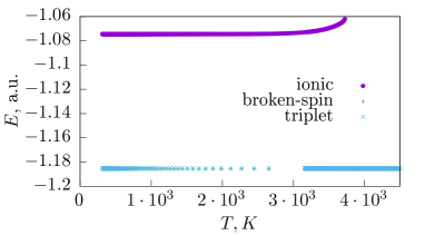
Figure 2: The temperature dependence of the GW internal energy and entropy for the H₂ molecule. The solutions are labeled according to the physical meaning of the corresponding HF solutions.

H₂ molecule. We obtained 3 zero-temperature Hartree–Fock solutions for a stretched hydrogen molecule: broken-spin UHF, high-spin UHF (triplet), and RHF (ionic) solutions. Using these HF solutions as guesses, we converged the corresponding unrestricted and restricted finite-temperature self-consistent HF, GW, and GF2 calculations. The resulting finite-temperature solutions are distinct from each other. To obtain these solutions as a function of temperature, the chemical potential is optimized at $\beta=1000$ a.u.^-1 separately for each of the solutions to ensure that $n=2$, where $n$ is the number of electrons. Subsequently, the chemical potential was fixed at this value for all other temperatures. The energies and entropies for the GW solutions (Figure 2) are flat in a broad range of temperatures. At a very high temperature, the GW solution obtained from RHF (ionic) solution starts losing electrons (due to maintaining a constant chemical potential for all temperatures), which leads to an increase in the energy and entropy (see Figure 2).

Table 1: Local charge and spin correlators for the H₂ molecule, computed for Green’s functions at $\beta=1000$ a.u. Both full GW and only disconnected part of the GW correlators are are listed.

$\mathbf{\braket{\delta N_{A}\delta N_{B}}}$				$\mathbf{\braket{\delta N_{A}\delta N_{A}}}$
method	ionic	triplet	broken-spin	method	ionic	triplet	broken-spin
HF (finite temp)	-0.38	0.00	0.00	HF (finite temp)	0.50	0.00	0.00
GW, disc	-0.28	0.00	0.00	GW, disc	0.51	0.01	0.01
GW	0.13	0.00	0.00	GW	0.64	0.30	0.30
GF2	-0.17	0.00	0.00	GF2	0.21	0.00	0.00
$\mathbf{\braket{\bar{S}_{A}\bar{S}_{B}}}$				$\mathbf{\braket{\bar{S}_{A}\bar{S}_{A}}}$
method	ionic	triplet	broken-spin	method	ionic	triplet	broken-spin
HF (finite temp)	-0.39	0.25	-0.25	HF (finite temp)	0.38	0.76	0.76
GW, disc	-0.28	0.25	-0.25	GW, disc	0.39	0.76	0.76
GW	-0.07	0.25	-0.25	GW	0.60	0.83	0.83
GF2	0.00	0.25	-0.25	GF2	0.61	0.76	0.76

Tab. 1 shows local charge and spin correlators between the same and different centers. Values of these correlators can be used to interpret and distinguish different molecular solutions as illustrated in Fig. 1. The zero-temperature RHF (ionic) solution is a mixture of covalent ($\braket{\delta N_{A}\delta N_{B}}=0$) and charge-resonance configurations ($\braket{\delta N_{A}\delta N_{B}}\neq 0$). Correlators, computed with the finite-temperature RHF solution, also show mixed charge-resonance and covalent characters. Characters of both finite-temperature UHF solutions also match the corresponding zero-temperature UHF solutions. These trends can be explained through a symmetry breaking of a particular type:

$$\hat{\rho}=\sum_{i}w_{i}\ket{\Psi_{i}}\bra{\Psi_{i}}\rightarrow\hat{\rho}_{HF}^{(T=0)}=\ket{\Phi_{HF}}\bra{\Phi_{HF}},$$ (16)

where $\hat{\rho}$ is the grand canonical density operator, $w_{i}$ are the Boltzmann weights for an eigenstate $\Psi_{i}$, and $\Phi_{HF}$ is the Hartree–Fock determinant (the last equality is written in the low-temperature limit). In general, when the symmetry breaking occurs, it does not result in a pure-state low-temperature limit, as is the case, for example, for HF with fractional occupancies. The corresponding symmetry analysis of $\hat{\rho}$ requires consideration of projective representations of symmetry groups rather than linear representations. This gives more pathways of symmetry breaking, going beyond Fukutome’s HF symmetry breaking classificationFukutome:UHF:81 (see also generalization for Green’s functionsMochena:Fukutome:broken_symmetry:GF ). However, in our case, we observe symmetry breaking with the pure-state low-temperature limit which is easy to analyze.

At zero temperature, the high-spin triplet UHF determinant describes the triplet wave function qualitatively correctly. However, the corresponding finite-temperature $\hat{\rho}$ should contain contributions from triplet configurations with all spin projections (since their energies are degenerate), requiring a multiconfigurational treatment. This results in a triplet symmetry-broken finite temperature UHF solution with unequal average numbers of $\alpha$ and $\beta$ electrons while having a triplet pure-state UHF solution in the low-temperature limit. For the finite temperature symmetry-broken triplet, local spin correlators are $0.76$ and $0.25$ for the spins on the same and different centers, respectively. The broken-spin UHF determinant leads to a broken-spin finite-temperature UHF solution with equal average numbers of $\alpha$ and $\beta$ electrons. While the local spin correlator on the same centers is $0.76$, the local spin correlator between different centers is $-0.25$ due to the opposite orientation of local spins in the broken-spin solution. Local charge correlators for both UHF solutions are zero, confirming the covalent character of these solutions.

GW and GF2 preserve the characters of the broken-spin UHF, high spin UHF, and RHF ionic solutions. Their energy and entropy temperature dependences are too flat (see Figure 2) because these methods do not provide enough correlation to properly illustrate temperature dependencies of these solutions (FCI does not have this issue as shown in Fig. S1 in SI). Although weakly correlated methods can give expressions for the density operator analogous to Eq. 16, one should be careful with such generalizations, since Green’s function methods do not have to be ensemble representatable. For example, the GW two-particle density matrix does not have the permutational symmetry required to ensure ensemble representability. Yet, local correlators provide useful characterizations for the solutions obtained. Different-center spin correlators evaluated for GW and GF2 obtained from the RHF (ionic) guess become closer to zero. The different-center charge correlators for this ionic solution range from $-0.38$ (HF) to $0.13$ (GW) and $-0.17$ (GF2) indicating that the presence of electronic correlation suppresses the high-energy ionic contributions and enhances the covalent character of the solution. This is also suggested by the increase in the local same-center spin correlators from $0.38$ (HF) to $0.60$ (GW) and $0.61$ (GF2). Although these correlators show an improvement in the description of strong correlation, the deviation from their limiting values is still significant, indicating that the solutions are partly contaminated with the ionic contributions. The above analysis explains why the restricted GF2 does not give correct electronic energies at the dissociation limit.

GF2 and GW solutions obtained from the UHF guesses preserve the character of the corresponding Hartree–Fock solutions. However, same-center GW correlators (the charge and spin correlators are 0.30 and 0.83, respectively) show deviations from the expected values. This artifact appears only when the electronic cumulant is present indicating that it is likely due to the omission of the correct permutational structure of the GW cumulant. This observation is consistent with our earlier findings of large charge and spin fluctuations in the atomic GW calculationsPokhilko:tpdm:2021 . The GF2 cumulant has a correct permutational structure and does not lead to these artifacts. Since the same-center correlators for the triplet and broken-spin GW solutions are numerically close, we hope that these effects will be cancelled when energy differences are considered.

The interpretation of energies of broken-spin UHF and DFT solutions was pioneered by Noodlemannoodleman:BS:81 , who suggested to construct effective Heisenberg Hamiltonians from such solutions. This approach found its widespread use in the evaluations of magnetic couplings for molecular magnetsNoodleman:BS:1986 ; Ruiz:BSDFT:99 ; Nishino:BSDFT:97 ; Soda:BSDFT:00 ; sinnecker:BS:Mn:04 . However, a rigorous theoretical justification of such a scheme is not always clear since the evaluation of two-particle properties in DFT is usually done for the Kohn–Sham determinant, which is not exactCremer:DFT:S2:2001 ; Handy:DFT:S2:2007 ; Vedene:DFT:S2:1995 . Here, we are following the Davidson’s and Clark’sDavidson:local_spin:2001 ; Davidson:local_spin:2002 ; Davidson:MolMagnets:2002 reasoning and use local spin correlators to construct the Heisenberg Hamiltonian and use the known relations between the effective exchange coupling $J$ and energy differences:

$$H=-J_{AB}\mathbf{S}_{A}\cdot\mathbf{S}_{B},$$

$$J=E(S)-E(T)=2\left(E(BS)-E(T)\right),$$

where S, T, and BS denote the singlet, triplet, and broken-spin solutions. Such construction of effective Hamiltonian is different from the Bloch’s effective Hamiltonian theoryBloch:1958 ; Cloizeax:1960 ; Okubo:1954 , also used for derivations of the effective magnetic HamiltoniansCalzado:02 ; Guihery:2009 ; Malrieu:2010 ; Marlieu:MagnetRev:2014 ; Mayhall:2014:HDVV ; Mayhall:1SF:2015 ; Pokhilko:EffH:2020 ; Pokhilko:spinchain .

Tab. 2 contains the extracted effective exchange couplings from the broken-spin and FCI solutions.

Table 2: Extracted parameters from FCI and broken-spin solutions in cm^-1.

System	Parameter	FCI	GW	GF2	UHF
H2	$J$	-213	-217	-218	-212
H4	$J$	-185	-189	-189	-183
H4	$J_{4c}$	-3.9	-3.8	-3.8	-3.4

The Noodleman’s interpretation applied to UHF, GW, and GF2 predicts exchange constants differing from the FCI ones by only a few wavenumbers.

Tetrahedral H₄. Stretched tetrahedral H₄ is another example of a strongly correlated system. Its Hartree–Fock broken-symmetry solutions has been classified beforeFukutome:H4:1975 ; Scuseria:magnetic:density:2018 . Here, we consider only the unrestricted solutions computed from axial UHF guesses. Similarly to the stretched H₂ molecule, all different-center spin correlators are close to $0.25$ and $-0.25$. The low-energy physics can be reconstructed through the following effective Hamiltonian:

$$H=-J\sum_{i<j}\mathbf{S}_{i}\cdot\mathbf{S}_{j}-J_{4c}\sum_{\braket{ijkl}}(\mathbf{S}_{i}\cdot\mathbf{S}_{j})(\mathbf{S}_{k}\cdot\mathbf{S}_{l}),$$

where the first term is the usual Heisenberg term while the second one is the four-spin-four-center interaction describing a deviation from the Heisenberg model. The summation in the second term runs over a unique partitioning of such indices: (12,34), (13,24), (14,23), where each of the numbers enumerates a radical center. The eigenvalues of this Hamiltonian are:

$$E(S=2) = -\frac{3}{2}J-\frac{3}{16}J_{4c}$$

$$E(S=1) = \frac{1}{2}J+\frac{5}{16}J_{4c}$$

$$E(S=0) = \frac{3}{2}J-\frac{15}{16}J_{4c}.$$

Broken-spin configurations are described by the diagonal of this model in a basis of determinants. The corresponding energies of the broken-spin configurations are:

$$E(S_{z}=\pm 2) = -\frac{3}{2}J-\frac{3}{16}J_{4c}$$

$$E(S_{z}=\pm 1) = 0+\frac{3}{16}J_{4c}$$

$$E(S_{z}=\pm 0) = \frac{1}{2}J-\frac{3}{16}J_{4c}.$$

Table 3: Energies of broken-spin solutions in cm^-1. The high-spin solutions are taken as a zero energy.

	GW	GF2	UHF
$S_{z}=0$	-378	-379	-366
$S_{z}=1$	-285	-286	-276
$S_{z}=2$	0	0	0

There are many degenerate broken-spin solutions, namely 4 solutions with $S_{z}=1$, 6 solutions with $S_{z}=0$, and only one high-spin solution with $S_{z}=2$. Such a high degree of degeneracy becomes clear if one looks at linear combinations of the spin-complete wave-functions, which mix into broken-spin configurations. Each $S_{z}=1$ or $S_{z}=0$ broken-spin configuration has contributions from wave-functions belonging to different irreducible representations of the $T_{d}$ tetrahedral point group. Thus, the broken-spin configurations form a larger, reducible representation. The energies of the broken-spin solutions, the extracted $J$ and $J_{4c}$ parameters, and the reconstructed energies are shown in Tables 3, 2, and 4. Extracted parameters and interpreted energies of GW, GF2, and UHF are very close to FCI. While H₂ and H₄ are toy examples that provide a basic validation for the exchange coupling constants extracted from UHF, GW, and GF2, realistic, many-electron, strongly correlated systems are more complex. In these systems, UHF $\braket{S^{2}}$ may significantly differ from the values, expected from the Noodleman’s interpretation.

Below we consider two more complicated transition metal complexes with electronic structure qualitatively resembling the Heisenberg Hamiltonian.

Table 4: FCI energies and constructed energies from broken-spin solutions in cm^-1. The high-spin solutions are taken as a zero energy.

Symmetry	FCI	GW	GF2	UHF
1E	-552	-564	-565	-546
3T2	-372	-380	-381	-368
5A1	0	0	0	0

Table 5: A comparison between effective exchange constants (in cm^-1) extracted from the broken-spin GW, wave-function theories, and experiments.

Complex	BS-UHF	BS-GW	WF theories	Exp.
Cu2Cl${}_{6}^{2-}$	$-57.4$	$-48.8$	$-16$ a	0, $-40$Caballol:Cu_struct:1994
Fe2OCl${}_{6}^{2-}$	$-44.4$	$-164.1$	$-125.4$..$-108.6$ $-250.2$..$-226.8$ $-233.6$..$-190.8$ b	$-234$Molins:Fe2OCl6:magnet:2003

^a EOM-SF-CCSDOrms:magnets:17
^b Ranges of effective exchange constants (CASSCF, MRCI+Q, DMRG, respectively), extracted from the pairs of states with $\Delta S=1$Morokuma:DMRG:biquad_exc:2014 .

Transition metal complexes: [Cu₂Cl₆]^2- and [Fe₂OCl₆]^2-. Geometries of [Fe₂OCl₆]^2- and [Cu₂Cl₆]^2- were taken from their crystal structures Molins:fe_struct:1998 ; Caballol:Cu_struct:1994 , and are consistent with previous theoretical studies Morokuma:DMRG:biquad_exc:2014 ; Orms:magnets:17 . Similar to the H₂ molecule, we obtained the high-spin and broken-spin UHF and GW solutions for both [Cu₂Cl₆]^2- and [Fe₂OCl₆]^2-. Using the Noodleman’s interpretation of broken-spin solutions, the extracted antiferromagnetic effective exchange couplings $J$ agree with the experimental results and previous theoretical studies (see Tab. 5). The exchange couplings $J$ for the copper complex, computed with the broken-spin UHF and GW, are close to the experimental results and EOM-SF-CCSD. The absolute value of $|J|$ decreases from UHF to GW possibly indicating that capturing of the weak correlation in [Cu₂Cl₆]^2- leads to a decrease of $|J|$. It explains why GW slightly overestimates $|J|$ with respect to a higher-level EOM-SF-CCSD calculation and the available experimental data. As discussed in the Ref.Morokuma:DMRG:biquad_exc:2014 , the treatment of weak correlation is important for a correct estimate of the exchange coupling in the iron complexes (explaining why UHF and CASSCF numbers are significantly different than the experimental estimate). The BS-GW estimate lies in between CASSCF and DMRG estimates. The increase in $|J|$ from UHF to GW is consistent with the previous theoretical calculations. The significant role of weak correlation is not unique to this iron example and has been observed before CuAc:Neese:2011 ; Pokhilko:spinchain .

The changes in electronic structure can be understood by means of local correlators. Davidson and Clark Davidson:local_spin:2001 noted that same-center correlators often give unrealistic values for the local spin due to closed-shell doubly occupied orbitals. The problem is exacerbated when core orbitals are not frozen or when effective core potentials are not used. They proposed to use differences of the correlators for the analysis of the energy differences. Since GW is not an ensemble respresentable method, its total $\braket{S^{2}}$ and $\braket{N^{2}}$ also do not have to be realistic. However, we see that this error cancels out if the differences are considered. For example, squared fluctuation of the number of particles $\braket{(\delta N)^{2}}$, computed for Cu₂Cl${}_{6}^{2-}$ with triplet and broken-spin GW solutions are $23.0019$ and $23.0046$ respectively. While these fluctuations do not describe a realistic system in the low-temperature limit, their difference is close to zero, justifying its use in the interpretation of energy differences. The difference between $\braket{S^{2}}$ of the high-spin and broken-spin GW solutions, $\braket{S^{2}}(\text{high spin})-\braket{S^{2}}(\text{bs})$, is $0.9995$ and $25.019$ for copper and iron complexes, respectively, which are close to the expected values from the broken-spin physics.

Tables S1–S8 in SI show spin and charge correlators computed for [Cu₂Cl₆]^2- and [Fe₂OCl₆]^2-. For [Cu₂Cl₆]^2-, the differences between UHF spin correlators are small, except the correlator between two different copper centers. The difference in spin correlators between copper and neighboring chlorine atoms are about 40 times larger than the difference in correlators between copper and distant chlorine atoms. The difference in charge correlators is small for all atom pairs indicating that the charge fluctuations for the both electronic states are similar and confirming the validity of the Heisenberg form of the effective Hamiltonian. The inclusion of electronic correlation through GW slightly increases the difference in spin correlators between different copper and chlorine centers preserving the Heisenberg form of effective interactions. This results only in a small change of the effective exchange coupling.

UHF difference in spin correlators for [Fe₂OCl₆]^2- is similar to the copper complex. While the difference in spin correlators for the same iron centers is small, the difference in spin correlators for the adjacent Fe and Cl or O centers is significant. This can be rationalized through a larger value of the local spin on an iron center (each Fe has 5 unpaired electrons) resulting in an increase of the correlators between iron and chlorine centers. The difference in charge correlators is small for all atoms except the oxygen center, which means that charge fluctuations on oxygen may influence the value of the effective exchange coupling. GW gives a qualitatively different picture. First, the difference in the same-center iron spin correlators increases by two orders of magnitude and becomes non-negligible ($\Delta\braket{\vec{S}_{A}\vec{S}_{B}}=0.16$). Second, the charge correlator between the same and different iron centers increases by an order of magnitude and becomes comparable to the one on the oxygen center. Consequently, this pronounced effect in charge correlators indicates that the electronic structure of the high-spin and low-spin electronic states influences additional configurations than just the main ones, resulting in a larger deviation between the broken-spin UHF and GW values. Another consequence is the expected deviation from the Heisenberg interaction form. Partial differential charge resonance between iron and bridging oxygen centers indicates that the interaction between the leading configurations and the charge-transfer configurations is significant, which can be wrapped into an effective biquadratic spin interaction (as shown through analysis of DFT calculations in Ref. Malrieu:DFT:biquad:2008 ). This observation explains previous multireference results Morokuma:DMRG:biquad_exc:2014 , parametrizing the biquadratic interaction.

To conclude, we applied a local analysis of electronic structure to Green’s function methods by means of local spin and charge correlators. These correlators quantify the covalent and ionic nature of the Green’s function solutions obtained. We found that weakly correlated self-consistent GW and GF2 are prone to symmetry breaking in open-shell cases, leading to solutions that do not change significantly with temperature. The analysis of these solutions allowed us to construct effective Heisenberg Hamiltonians, four-spin-four-center interactions, and explain trends in selected single-molecule magnets.

Supplementary Material

FCI temperature dependence of energy and entropy for H₂, two-particle charge and spin correlators for transition metal complexes, Cartesian geometries.

References

- (1) C. D. Roberts and A. G. Williams, Dyson-Schwinger equations and their application to hadronic physics, Prog. Part. Nucl. Phys. 33, 477 (1994).
- (2) C. D. Roberts and S. M. Schmidt, Dyson-Schwinger equations: Density, temperature and continuum strong QCD, Prog. Part. Nucl. Phys. 45, S1 (2000).
- (3) M. Nakano, A. Hasegawa, H. Kouno, and K. Koide, Nuclear Schwinger-Dyson formalism applied to finite baryon density. I. Formulation, Phys. Rev. C 49, 3061 (1994).
- (4) A. Stan, N. E. Dahlen, and R. van Leeuwen, Fully self-consistent GW calculations for atoms and molecules, EPL 76, 298 (2006).
- (5) N. E. Dahlen and R. van Leeuwen, Self-consistent solution of the Dyson equation for atoms and molecules within a conserving approximation, J. Chem. Phys. 122, 164102 (2005).
- (6) J. V. Ortiz, Electron propagator theory: an approach to prediction and interpretation in quantum chemistry, WIREs: Comput. Mol. Sci. 3, 123 (2013).
- (7) G. D. Mahan, Many-Particle Physics, Physics of Solids and Liquids. Springer, 2000.
- (8) J. W. Negele and H. Orland, Quantum many-particle systems. CRC Press, 2018.
- (9) R. M. Martin, L. Reining, and D. M. Ceperley, Interacting electrons. Cambridge University Press, 2016.
- (10) E. Kozik, M. Ferrero, and A. Georges, Nonexistence of the luttinger-ward functional and misleading convergence of skeleton diagrammatic series for hubbard-like models, Phys. Rev. Lett. 114, 156402 (2015).
- (11) W. Tarantino, P. Romaniello, J. A. Berger, and L. Reining, Self-consistent Dyson equation and self-energy functionals: An analysis and illustration on the example of the Hubbard atom, Phys. Rev. B 96, 045124 (2017).
- (12) R. Rossi and F. Werner, Skeleton series and multivaluedness of the self-energy functional in zero space-time dimensions, J. Phys. A: Math. Theor. 48, 485202 (2015).
- (13) A. Stan, P. Romaniello, S. Rigamonti, L. Reining, and J. A. Berger, Unphysical and physical solutions in many-body theories: from weak to strong correlation, New J. Phys. 17, 093045 (2015).
- (14) L. Salem and C. Rowland, The electronic properties of diradicals, Angew. Chem., Int. Ed. 11, 92 (1972).
- (15) M. A. El-Sayed, Triplet state: Its radiative and non-radiative properties, Acc. Chem. Res. 1, 8 (1968).
- (16) J. C. Johnson, A. J. Nozik, and J. Michl, The role of chromophore coupling in singlet fission, Acc. Chem. Res. 46, 1290 (2013).
- (17) J. Linderberg and Y. Öhrn, Propagators in quantum chemistry. Academic, London, 1973.
- (18) J. V. Ortiz, Toward an exact one-electron picture of chemical bonding, Adv. Quantum Chem. 35, 33 (1999).
- (19) C. M. Oana and A. I. Krylov, Dyson orbitals for ionization from the ground and electronically excited states within equation-of-motion coupled-cluster formalism: Theory, implementation, and examples, J. Chem. Phys. 127, 234106 (2007).
- (20) A. V. Luzanov, A. A. Sukhorukov, and V. E. Umanskii, Application of transition density matrix for analysis of excited states, Theor. Exp. Chem. 10, 354 (1976), Russian original: Teor. Eksp. Khim., 10, 456 (1974).
- (21) A. V. Luzanov and V. F. Pedash, Interpretation of excited states using charge-transfer number, Theor. Exp. Chem. 15, 338 (1979).
- (22) M. Head-Gordon, A. M. Grana, D. Maurice, and C. A. White, Analysis of electronic transitions as the difference of electron attachment and detachment densities, J. Phys. Chem. 99, 14261 (1995).
- (23) R. L. Martin, Natural transition orbitals, J. Phys. Chem. A 118, 4775 (2003).
- (24) A. V. Luzanov and O. A. Zhikol, Excited state structural analysis: TDDFT and related models, in Practical aspects of computational chemistry I: An overview of the last two decades and current trends, edited by J. Leszczynski and M.K. Shukla, pages 415–449. Springer, 2012.
- (25) F. Plasser, M. Wormit, and A. Dreuw, New tools for the systematic analysis and visualization of electronic excitations. I. formalism, J. Chem. Phys. 141, 024106 (2014).
- (26) F. Plasser, S. A. Bäppler, M. Wormit, and A. Dreuw, New tools for the systematic analysis and visualization of electronic excitations. II. Applications, J. Chem. Phys. 141, 024107 (2014).
- (27) K. D. Nanda and A. I. Krylov, Visualizing the contributions of virtual states to two-photon absorption cross-sections by natural transition orbitals of response transition density matrices, J. Phys. Chem. Lett. 8, 3256 (2017).
- (28) W. Skomorowski and A. I. Krylov, Real and imaginary excitons: Making sense of resonance wavefunctions by using reduced state and transition density matrices, J. Phys. Chem. Lett. 9, 4101 (2018).
- (29) S. Mewes, F. Plasser, A. I. Krylov, and A. Dreuw, Benchmarking excited-state calculations using exciton properties, J. Chem. Theory Comput. 14, 710 (2018).
- (30) S. A. Mewes and A. Dreuw, Density-based descriptors and exciton analyses for visualizing and understanding the electronic structure of excited states, Phys. Chem. Chem. Phys. 21, 2843 (2019).
- (31) P. Pokhilko and A. I. Krylov, Quantitative El-Sayed rules for many-body wavefunctions from spinless transition density matrices, J. Phys. Chem. Lett. 10, 4857 (2019).
- (32) A. I. Krylov, From orbitals to observables and back, J. Chem. Phys. 153, 080901 (2020).
- (33) K. D. Nanda and A. I. Krylov, A simple molecular orbital picture of RIXS distilled from many-body damped response theory, J. Chem. Phys. 152, 244118 (2020).
- (34) K. D. Nanda and A. I. Krylov, The Orbital Picture of the First Dipole Hyperpolarizability from Many-Body Response Theory, (2021).
- (35) R. D. Harcourt, G. D. Scholes, and K. P. Ghiggino, Rate expressions for excitation transfer. II. Electronic considerations of direct and through-configuration exciton resonance interactions, J. Chem. Phys. 101, 10521 (1994).
- (36) S. M. Parker, T. Seideman, M. Ratner, and T. Shiozaki, Communication: Active-space decomposition for molecular dimers, J. Chem. Phys. 139, 021108 (2013).
- (37) S. M. Parker and T. Shiozaki, Quasi-diabatic states from active space decomposition, J. Chem. Theory Comput. 10, 3738 (2014).
- (38) N. A. Besley, D. P. O’Neill, and P. M. W. Gill, Computation of molecular Hartree–Fock Wigner intracules, J. Chem. Phys. 118, 2033 (2003).
- (39) N. A. Besley and P. M. W. Gill, Atomic and molecular intracules for excited states, J. Chem. Phys. 120, 7290 (2004).
- (40) A. V. Luzanov and O. V. Prezhdo, Analysis of multiconfigurational wave functions in terms of hole-particle distributions, J. Chem. Phys. 124, 224109 (2006).
- (41) T. Juhász and D. A. Mazziotti, The cumulant two-particle reduced density matrix as a measure of electron correlation and entanglement, J. Chem. Phys. 125, 174105 (2006).
- (42) P. Kimber and F. Plasser, Toward an understanding of electronic excitation energies beyond the molecular orbital picture, Phys. Chem. Chem. Phys. 22, 6058 (2020).
- (43) P. Pokhilko, S. Iskakov, C.-N. Yeh, and D. Zgid, Evaluation of two-particle properties within finite-temperature self-consistent one-particle Green’s function methods: theory and application to GW and GF2, 2021.
- (44) L. J. Holleboom and J. G. Snijders, A comparison between the Möller–Plesset and Green’s function perturbative approaches to the calculation of the correlation energy in the many-electron problem, J. Chem. Phys. 93, 5826 (1990).
- (45) J. J. Phillips and D. Zgid, Communication: The description of strong correlation within self-consistent Green’s function second-order perturbation theory, J. Chem. Phys. 140, 241101 (2014).
- (46) A. A. Rusakov and D. Zgid, Self-consistent second-order Green’s function perturbation theory for periodic systems, J. Chem. Phys. 144, 054106 (2016).
- (47) A. R. Welden, A. A. Rusakov, and D. Zgid, Exploring connections between statistical mechanics and green’s functions for realistic systems: Temperature dependent electronic entropy and internal energy from a self-consistent second-order green’s function, J. Chem. Phys. 145, 204106 (2016).
- (48) S. Iskakov, A. A. Rusakov, D. Zgid, and E. Gull, Effect of propagator renormalization on the band gap of insulating solids, Phys. Rev. B 100, 085112 (2019).
- (49) L. Hedin, New method for calculating the one-particle Green’s function with application to the electron-gas problem, Phys. Rev. 139, A796 (1965).
- (50) W. E. Pickett and C. S. Wang, Local-density approximation for dynamical correlation corrections to single-particle excitations in insulators, Phys. Rev. B 30, 4719 (1984).
- (51) M. S. Hybertsen and S. G. Louie, Electron correlation in semiconductors and insulators: Band gaps and quasiparticle energies, Phys. Rev. B 34, 5390 (1986).
- (52) F. Aryasetiawan and O. Gunnarsson, The GW method, Rep. Prog. Phys. 61, 237 (1998).
- (53) P. Koval, D. Foerster, and D. Sánchez-Portal, Fully self-consistent GW and quasiparticle self-consistent GW for molecules, Phys. Rev. B 89, 155417 (2014).
- (54) A. Kutepov, Sergey Y. Savrasov, and G. Kotliar, Ground-state properties of simple elements from GW calculations, Phys. Rev. B 80, 041103(R) (2009).
- (55) R. Kubo, Generalized cumulant expansion method, J. Phys. Soc. Jap. 17, 1100 (1962).
- (56) K. Ruedenberg, The physical nature of the chemical bond, Rev. Mod. Phys. 34, 326 (1962).
- (57) M. S. de Giambiagi, M. Giambiagi, and F. E. Jorge, Bond index: relation to second-order density matrix and charge fluctuations, Theor. Chim. Acta 68, 337 (1985).
- (58) A. Torre, L. Lain, R. Bochicchio, and R. Ponec, Topological population analysis from higher order densities II. the correlated case, J. Math. Chem. 32, 241 (2002).
- (59) A. Torre, L. Lain, and R. Bochicchio, Bond orders and their relationships with cumulant and unpaired electron densities, J. Phys. Chem. A 107, 127 (2003).
- (60) T. Yamasaki and W. A. Goddard, Correlation analysis of chemical bonds, J. Phys. Chem. A 102, 2919 (1998).
- (61) A. V. Luzanov and O. V. Prezhdo, Irreducible charge density matrices for analysis of many-electron wave functions, Int. J. Quant. Chem. 102, 582 (2005).
- (62) I. Mayer, Bond order and valence indices: A personal account, J. Comput. Chem. 28, 204 (2007).
- (63) A. E. Clark and E. R. Davidson, Local spin, J. Chem. Phys. 115, 7382 (2001).
- (64) E. R. Davidson and A. E. Clark, Local spin II, Mol. Phys. 100, 373 (2002).
- (65) E. R. Davidson and A. E. Clark, Model molecular magnets, J. Phys. Chem. A 106, 7456 (2002).
- (66) C. Herrmann, M. Reiher, and B. A. Hess, Comparative analysis of local spin definitions, J. Chem. Phys. 122, 034102 (2005).
- (67) A. V. Luzanov, D. Casanova, X. Feng, and A. I. Krylov, Quantifying charge resonance and multiexciton character in coupled chromophores by charge and spin cumulant analysis, J. Chem. Phys. 142, 224104 (2015).
-
(68)
Note that the localized basis is non-orthogonal. In the non-orthogonal
orbitals, the second-quantized anticommutation
relationsSurjan:Secquant:2012 between creation and annihilation
operators can be expressed as
where is the overlap matrix between non-orthogonal orbitals. Operators are written through the corresponding integrals and creation and annihilation operators.(17) (18) - (69) T. H. Dunning, Jr., Gaussian basis sets for use in correlated molecular calculations. I. The atoms boron through neon and hydrogen, J. Chem. Phys. 90, 1007 (1989).
- (70) D. E. Woon and T. H. Dunning, Gaussian basis sets for use in correlated molecular calculations. III. The atoms aluminum through argon, J. Chem. Phys. 98, 1358 (1993).
- (71) N. B. Balabanov and K. A. Peterson, Systematically convergent basis sets for transition metals. I. All-electron correlation consistent basis sets for the 3d elements Sc-Zn, J. Chem. Phys. 123, 064107 (2005).
- (72) S. Iskakov, C.-N. Yeh, E. Gull, and D. Zgid, Ab initio self-energy embedding for the photoemission spectra of NiO and MnO, Phys. Rev. B 102, 085105 (2020).
- (73) Q. Sun, T. C. Berkelbach, N. S. Blunt, G. H. Booth, S. Guo, Z. Li, J. Liu, J. D. McClain, E. R. Sayfutyarova, S. Sharma, S. Wouters, and G. K. Chan, Pyscf: the python-based simulations of chemistry framework, Wiley Interdiscip. Rev.: Comput. Mol. Sci. 8, e1340 (2017).
- (74) G. M. J. Barca, C. Bertoni, L. Carrington, D. Datta, N. De Silva, J. E. Deustua, D. G. Fedorov, J. R. Gour, A. O. Gunina, E. Guidez, T. Harville, S. Irle, J. Ivanic, K. Kowalski, S. S. Leang, H. Li, W. Li, J. J. Lutz, I. Magoulas, J. Mato, V. Mironov, H. Nakata, B. Q. Pham, P. Piecuch, D. Poole, S. R. Pruitt, A. P. Rendell, L. B. Roskop, K. Ruedenberg, T. Sattasathuchana, M. W. Schmidt, J. Shen, L. Slipchenko, M. Sosonkina, V. Sundriyal, A. Tiwari, J. L. Galvez Vallejo, B. Westheimer, M. Wloch, P. Xu, F. Zahariev, and M. S. Gordon, Recent developments in the general atomic and molecular electronic structure system, J. Chem. Phys. 152, 154102 (2020).
- (75) H. Fukutome, Unrestricted Hartree-Fock method and its applications to molecules and chemical reactions, Int. J. Quant. Chem. 20, 955 (1981).
- (76) A. K. Rajagopal and M. Mochena, Broken-symmetry-adapted Green function theory of condensed matter systems: Towards a vector spin-density-functional theory, Phys. Rev. B 62, 15461 (2000).
- (77) L. Noodleman, Valence bond description of antiferromagnetic coupling in transition metal dimers, J. Chem. Phys. 74, 5737 (1981).
- (78) L. Noodleman and E. R. Davidson, Ligand spin polarization and antiferromagnetic coupling in transition metal dimers, Chem. Phys. 109, 131 (1986).
- (79) E. Ruiz, J. Cano, S. Alvarez, and P. Alemany, Broken symmetry approach to calculation of exchange coupling constants for homobinuclear and heterobinuclear transition metal complexes, J. Comput. Chem. 20, 1391 (1999).
- (80) M. Nishino, S. Yamanaka, Y. Yoshioka, and K. Yamaguchi, Theoretical approaches to direct exchange couplings between divalent chromium ions in naked dimers, tetramers, and clusters, J. Phys. Chem. A 101, 705 (1997).
- (81) T. Soda, Y. Kitagawa, T. Onishi, Y. Takano, Y. Shigeta, H. Nagao, Y. Yoshioka, and K. Yamaguchi, Ab initio computations of effective exchange integrals for H–H, H–He–H and Mn2O2 complex: comparison of broken-symmetry approaches, Chem. Phys. Lett. 319, 223 (2000).
- (82) S. Sinnecker, F. Neese, L. Noodleman, and W. Lubitz, Calculating the electron paramagnetic resonance parameters of exchange coupled transition metal complexes using broken symmetry density functional theory: application to a Mn(III)/Mn(IV) model compound, J. Am. Chem. Soc. 126, 2613 (2004).
- (83) J. Gräfenstein and D. Cremer, On the diagnostic value of () in Kohn–Sham density functional theory, Mol. Phys. 99, 981 (2001).
- (84) A. J. Cohen, D. J. Tozer, and N. C. Handy, Evaluation of in density functional theory, J. Chem. Phys. 126, 214104 (2007).
- (85) J. Wang, A. D. Becke, and V. H. Smith, Evaluation of in restricted, unrestricted hartree–fock, and density functional based theories, J. Chem. Phys. 102, 3477 (1995).
- (86) C. Bloch, Sur la thèorie des perturbations des états liés, Nucl. Phys. 6, 329 (1958).
- (87) J. des Cloizeaux, Extension d’une formule de lagrange à des problèmes de valeurs propres, Nucl. Phys. 20, 321 (1960).
- (88) S. Ôkubo, Diagonalization of Hamiltonian and Tamm-Dancoff equation, Prog. Theor. Phys. 12, 603 (1954).
- (89) C. J. Calzado, J. Cabrero, J. P. Malrieu, and R. Caballol, Analysis of the magnetic coupling in binuclear complexes. II. Derivation of valence effective hamiltonians from ab initio CI and DFT calculations, J. Chem. Phys. 116, 3985 (2002).
- (90) R. Maurice, R. Bastardis, C. de Graaf, N. Suaud, T. Mallah, and N. Guihèry, Universal theoretical approach to extract anisotropic spin hamiltonians, J. Chem. Theory Comput. 5, 2977 (2009).
- (91) A. Monari, D. Maynau, and J.-P. Malrieu, Determination of spin Hamiltonians from projected single reference configuration interaction calculations. I. Spin 1/2 systems, J. Chem. Phys. 133, 044106 (2010).
- (92) J. P. Malrieu, R. Caballol, C. J. Calzado, C. de Graaf, and N. Guihéry, Magnetic interactions in molecules and highly correlated materials: Physical content, analytical derivation, and rigorous extraction of magnetic Hamiltonians, Chem. Rev. 114, 429 (2013).
- (93) N. J. Mayhall and M. Head-Gordon, Computational quantum chemistry for single Heisenberg spin couplings made simple: Just one spin flip required, J. Chem. Phys. 141, 134111 (2014).
- (94) N. J. Mayhall and M. Head-Gordon, Computational quantum chemistry for multiple-site Heisenberg spin couplings made simple: Still only one spin-flip required, J. Phys. Chem. Lett. 6, 1982 (2015).
- (95) P. Pokhilko and A. I. Krylov, Effective Hamiltonians derived from equation-of-motion coupled-cluster wave-functions: Theory and application to the Hubbard and Heisenberg Hamiltonians, J. Chem. Phys. 152, 094108 (2020).
- (96) P. Pokhilko, D. S. Bezrukov, and A. I. Krylov, Is solid copper oxalate a spin chain or a mixture of entangled spin pairs?, J. Phys. Chem. C 125, 7502 (2021).
- (97) H. Fukutome, M. Takahashi, and T. Takabe, The unrestricted hartree-fock theory of chemical reactions. IV: Singlet radical states with “antiferromagnetic” spin orderings in four-center exchange reaction of hydrogen molecules, Progr. Theor. Exp. Phys. 53, 1580 (1975).
- (98) T. M. Henderson, C. A. Jiménez-Hoyos, and G. E. Scuseria, Magnetic structure of density matrices, J. Chem. Theory Comput. 14, 649 (2018).
- (99) O. Castell, J. Miralles, and R. Caballol, Structural dependence of the singlet-triplet gap in doubly bridged copper dimers: a variational CI calculation, Chem. Phys. 179, 377 (1994).
- (100) A. Lledós, M. Moreno-Maas, M. Sodupe, A. Vallribera, I. Mata, B. Martínez, and E. Molins, Bent and linear forms of the (-oxo)bis[trichloroferrate(III)] dianion: An intermolecular effect–structural, electronic and magnetic properties, Eur. J. Inorg. Chem. 2003, 4187 (2003).
- (101) N. Orms and A. I. Krylov, Singlet-triplet energy gaps and the degree of diradical character in binuclear copper molecular magnets characterized by spin-flip density functional theory, Phys. Chem. Chem. Phys. 20, 13127 (2018).
- (102) T. V. Harris, Y. Kurashige, T. Yanai, and K. Morokuma, Ab initio density matrix renormalization group study of magnetic coupling in dinuclear iron and chromium complexes, J. Chem. Phys. 140, 054303 (2014).
- (103) E. Molins, A. Roig, C. Miravitlles, M. Moreno-Mañas, A. Vallribera, N. Gálvez, and N. Serra, Crystal and molecular structure of (BzlMe3N)2+[Fe2OCl6]2, Struct. Chem. 9, 203 (1998).
- (104) R. Maurice, K. Sivalingam, D. Ganyushin, N. Guihéry, C. de Graaf, and F. Neese, Theoretical determination of the zero-field splitting in copper acetate monohydrate, Inorg. Chem. 50, 6229 (2011).
- (105) P. Labèguerie, C. Boilleau, R. Bastardis, N. Suaud, N. Guihéry, and J.-P. Malrieu, Is it possible to determine rigorous magnetic hamiltonians in spin s=1 systems from density functional theory calculations?, J. Chem. Phys. 129, 154110 (2008).
- (106) P. R. Surján, Second quantized approach to quantum chemistry: an elementary introduction. Springer Berlin Heidelberg, 1989.