Simultaneous Wireless Information and Power Transfer for Federated Learning

Abstract

In the Internet of Things, learning is one of most prominent tasks. In this paper, we consider an Internet of Things scenario where federated learning is used with simultaneous transmission of model data and wireless power. We investigate the trade-off between the number of communication rounds and communication round time while harvesting energy to compensate the energy expenditure. We formulate and solve an optimization problem by considering the number of local iterations on devices, the time to transmit-receive the model updates, and to harvest sufficient energy. Numerical results indicate that maximum ratio transmission and zero-forcing beamforming for the optimization of the local iterations on devices substantially boost the test accuracy of the learning task. Moreover, maximum ratio transmission instead of zero-forcing provides the best test accuracy and communication round time trade-off for various energy harvesting percentages. Thus, it is possible to learn a model quickly with few communication rounds without depleting the battery.

I Introduction

Internet of Things (IoT) devices will arguably generate large amount of data, which can be of great use for prediction and inference in several applications of major societal interest [1]. Thus, it is natural to push machine learning solution into the Internet of Things (IoT) devices [2]. However, machine learning is traditionally conceived in centralized settings, where all data is available at one location. When we use machine learning on distributed wireless scenarios, such as the IoT applications, we encounter new challenges for both learning (such as heterogeneity of the data generated by the distributed devices and privacy issues [3]), and communication (such as communication efficiency, interference channel, fading, and battery limitations [4]).

Federated learning (FL) is a recently proposed distributed machine learning technique that attempts to overcome some of these challenges, since it enhances the privacy by sending only model updates instead of raw data, and considers the heterogeneity of devices data and the communication efficiency in the learning convergence [3]. For IoT scenarios, the limited energy storage capacity and high maintenance cost of devices battery is the main challenge [5]. To this end, federated learning (FL) in IoT scenarios must consider the battery of the devices as one of the most important aspects, together with the impact of communication efficiency, interference, and fading.

One promising solution to overcome the energy limitations in IoT is energy harvesting, which allows devices to harvest radio frequency energy when communicating with an edge server, e.g., a base station or access point [6]. Hence, the use of energy harvesting for IoT devices with FL would be a perfect combination. However, how to allow the devices to harvest sufficient energy to train a FL model is largely an open question. This idea is highly novel and, to the best of our knowledge, there is only one similar work in the literature [7]. In [7], the authors consider a wireless power transfer scenario served by power-beacons using FL. Such a work shows that higher density of power beacons improves the learning convergence, and that the mini-batch size and processor clock frequency is inversely proportional to the energy spent in local computation.

Different from the authors in [7], we investigate the trade-off among the number of communication rounds between an edge server and the IoT devices, and the communication round time necessary to train, transmit, and receive the model while harvesting sufficient energy to compensate part of the total energy spent. This trade-off is important to understand in which conditions we can train a FL task without depleting the battery of the devices. We consider a scenario with a multi-antenna edge server using the simultaneous wireless information and power transfer (SWIPT) technology with IoT devices using FL to simultaneously train a learning model, while communicating with an edge server (see Figure 1). Moreover, we consider the use of FedProx [8], a recent generalization of FL that allows to optimize the number of local iterations at each device, while guaranteeing convergence to (non-)convex learning tasks. We propose an optimization problem to minimize the number of communication rounds and communication round time while optimizing the number of local iterations, the time to transmit/receive, and to harvest a percentage of the total energy spent at each round and device.

Figure 1: An example of a network employing FL and SWIPT with $K$ devices. The devices send the weights $\mathbf{w}_{k}^{t-1}$ in the uplink, while the edge server sends the aggregated weight $\mathbf{w}^{t}$ and energy in the downlink.

We provide the solution to this problem while considering low transmit power at devices and fixed beamforming techniques, e.g., maximum ratio transmission (MRT) and zero-forcing (ZF), at the edge server. The results indicate that the learning test accuracy using either MRT or ZF with the optimization of the local number of iterations outperform a solution without such optimization. We also show that MRT vastly outperforms ZF in terms of minimum communication round time for all the percentage of the energy harvesting required. Therefore, we show that it is possible to use FL in IoT scenarios without depleting the battery of the devices.

Notation: Vectors and matrices are denoted by bold lower and upper case letters, respectively; ${\mathbf{A}}^{\mathrm{H}}$ is the Hermitian of $\mathbf{A}$; $\mathbf{I}_{K}$ is the identity matrix of dimension $K$; and by $\mathbb{C}$ the complex field. We denote expectation by $\mathbb{E}[\cdot]$; the uniform distribution with minimum and maximum parameters $a,b$, respectively, is denoted by $\mathcal{U}(a,b)$; the gradient of $f$ at $\mathbf{x}$ by $\nabla f(\mathbf{x})\in\mathbb{R}^{n}$; and the $2-$norm of a vector $\mathbf{x}$ by $\left\|\mathbf{x}\right\|$.

II System Model

We consider a general IoT scenario with an edge server equipped with $M$ antennas and $K$ single-antenna devices (see Figure 1). The devices represent sensors gathering data for an FL task and a power splitting SWIPT receiver architecture [6, 9]. In the following, we define the communication, energy, time, and learning models.

II-A Communication Model

Let $\mathbf{h}_{k}\in\mathbb{C}^{M\times 1}$ denote the uplink complex channel vector comprising small- and large-scale fading that includes the effects of multipath, shadowing, and path-loss between device $k$ and the edge server. The transmit power of device $k$ at the uplink is denoted as $p_{k}$, which is assumed fixed. The received signal at the edge server is given by

$$\overline{\mathbf{y}}^{u}=\sum\nolimits_{k=1}^{K}\mathbf{h}_{k}\sqrt{p_{k}}s_{k}^{u}+\mathbf{\boldsymbol{\eta}}^{u}\in\mathds{C}^{M\times 1},$$ (1)

where $s_{k}^{u}$ is the transmitted data symbol by device $k$ with zero mean and unit power; and $\mathbf{\boldsymbol{\eta}}^{u}\in\mathbb{C}^{M\times 1}$ is the additive white Gaussian noise with covariance matrix $\mathbb{E}\{\mathbf{\boldsymbol{\eta}}^{u}{\mathbf{\boldsymbol{\eta}}^{u}}^{\mathrm{H}}\}=\sigma^{2}\mathbf{I}_{M\times M}$. The signal-to-interference-plus-noise ratio (SINR) of the uplink device $k$ at the edge server is denoted as

$$\Gamma_{k}^{u}=\frac{p_{k}\left|{\mathbf{u}}^{\mathrm{H}}_{k}\mathbf{h}_{k}\right|^{2}}{\sum_{j\neq k}p_{j}\left|{\mathbf{u}}^{\mathrm{H}}_{k}\mathbf{h}_{j}\right|^{2}+\sigma^{2}},$$ (2)

where $\mathbf{u}_{k}$ is the uplink combiner at the edge server and is assumed fixed during the coherence time of the channel. In the uplink, the achievable rate of device $k$ is given by

$$R_{k}^{u}=B_{c}\log_{2}\left(1+\Gamma_{k}^{u}\right),$$ (3)

where $B_{c}$ denotes the channel bandwidth of each device.

In the downlink, the edge server aggregates the weight updates from all $k$ devices and unicasts the aggregated updates to each device $k$. The edge server applies a unicast transmission instead of multicast to increase the beamforming gain when harvesting the energy. The transmitted beamforming vector for device $k$ is denoted as $\mathbf{v}_{k}\in\mathbb{C}^{M\times 1}$, which is assumed fixed according to MRT or ZF. The received signal at device $k$ is given by

$$\overline{y}_{k}^{d}={\mathbf{h}}^{\mathrm{H}}_{k}\mathbf{v}_{k}s_{k}^{d}+\sum\nolimits_{j\neq k}{\mathbf{h}}^{\mathrm{H}}_{k}\mathbf{v}_{j}s_{j}^{d}+\eta^{d},$$ (4)

where $s_{k}^{d}$ is the transmitted data symbol to device $k$ with zero mean and unit power; and $\eta^{d}\in\mathbb{C}^{1}$ is the additive white Gaussian noise with variance $\mathbb{E}\{\left|\eta^{d}\right|^{2}\}=\sigma^{2}$. Note that we allow for different $s_{k}^{d}$ as transmitted symbols in Eq. (4), which reflect different coding between the devices. We denote by $P_{k}^{r}$ the received power at device $k$, which is given by

$$P_{k}^{r}=\sum\nolimits_{j=1}^{K}\left|{\mathbf{h}}^{\mathrm{H}}_{k}\mathbf{v}_{j}\right|^{2}+\sigma^{2}.$$ (5)

Note that depending on the beamforming $\mathbf{v}_{k}$, the received power changes drastically due to the cancellation or not of the multi-user interference in ZF and MRT, respectively. At device $k$, the receiver splits its received signal into the data detection and energy storage circuits. Let us denote the power splitting parameter for device $k$ as $\delta_{k}\in(0,1)$, which is fixed and indicates that $\delta_{k}P_{k}^{r}$ is directed to the data decoding unit and $(1-\delta_{k})P_{k}^{r}$ to the energy harvesting unit. During the baseband conversion, an additional circuit noise, denoted as $v_{i}$, is present due to the phase offsets and non-linearities, which is modelled as an additive white Gaussian noise with zero mean and variance $\sigma_{c}^{2}$. Thus, the SINR at device $k$ is given by

$$\Gamma_{k}^{d}=\frac{\delta_{k}\left|{\mathbf{h}}^{\mathrm{H}}_{k}\mathbf{v}_{k}\right|^{2}}{\delta_{k}\left(\sum_{j\neq k}\left|{\mathbf{h}}^{\mathrm{H}}_{k}\mathbf{v}_{j}\right|^{2}+\sigma^{2}\right)+\sigma_{c}^{2}}.$$ (6)

In the downlink, the achievable rate at device $k$ is given by

$$R_{k}^{d}=B_{c}\log_{2}\left(1+\Gamma_{k}^{d}\right).$$ (7)

II-B Energy and Time Models

We define the energy consumption to compute the model at device $k$ as [10]

$$E_{k}^{c}=\kappa C_{k}A_{k}I_{k}f_{k}^{2},$$ (8)

where $\kappa$ is the effective switched capacitance, $C_{k}$ is the number of central processing unit cycles required for computing one sample data at device in Mcycles/bit, $A_{k}$ is the dataset size in bits at device $k$, $I_{k}$ is the number of local iterations performed in the training phase by the learning algorithm, and $f_{k}$ is the processor clock frequency at device $k$ in GHz. Assuming that the uplink transmission occurs during $t_{k}^{u}$ seconds and the transmitted power is $p_{k}$, the energy to transmit the weights in the uplink is $E_{k}^{t}=t_{k}^{u}p_{k}$. Hence, the total energy spent at device $k$ during one communication round is $E_{k}^{c}+E_{k}^{t}$.

We consider a nonlinear energy harvesting model as in [11], in which the harvested power $P_{k}^{h}$ is given by

$$P_{k}^{h}=\alpha_{1}\left((1-\delta_{k})P_{k}^{r}\right)^{2}+\alpha_{2}\left((1-\delta_{k})P_{k}^{r}\right)+\alpha_{3},$$ (9)

where $\alpha_{1},\alpha_{2},\alpha_{3}\in\mathbb{R}$ are parameters of the model. We define the energy harvested at device $k$ as $E^{h}_{k}=t_{k}^{d}P_{k}^{h}$, where $t_{k}^{d}$ is the transmission time in seconds that the edge server spends to unicast the aggregated weight to device $k$. Therefore, we constraint the total energy spent by the total harvested energy at device $k$, i.e., $E_{k}^{t}+E_{k}^{c}\leq E^{h}_{k}$.

In the uplink, we assume that device $k$ has $D_{k}$ bits to transmit, corresponding to the dimension of the weight updates multiplied by the number of bits used to represent each dimension. Thus, each device $k$ has a constraint $t_{k}^{u}R_{k}^{u}\geq D_{k}$ in the uplink. Similarly, the downlink rate must ensure that the aggregated weight is unicasted to each device. Hence, each device $k$ has a constraint $t_{k}^{d}R_{k}^{d}\geq D_{k}$ in the downlink.

In addition, we need to take into account the time necessary for device $k$ to solve the local problem. Let us denote the time to solve the local training problem device $k$ as [10]

$$t_{k}^{c}=C_{k}A_{k}I_{k}/f_{k},$$ (10)

where $C_{k}$, $A_{k}$, $I_{k}$, and $f_{k}$ are the same parameters as in Eq. (8). Therefore, we denote the time for one communication round, including the uplink transmission with local computation, and downlink transmission with harvesting time, as $t^{r}=\max_{k}\;(t_{k}^{u}+t_{k}^{c})+\max_{k}\;(t_{k}^{d})$.

II-C Learning Model

The FL methods [3, 8] are designed to support multiple devices collecting data and a server (edge server in our case) coordinating the global learning objective for the network. The objective of the network is to solve the problem below:

$$\underset{\mathbf{w}}{\text{minimize}} f(\mathbf{w})=\sum\nolimits_{k=1}^{K}\frac{N_{k}}{N}F_{k}(\mathbf{w}),$$ (11)

where $N=\sum_{k=1}^{K}N_{k}$ and $\mathbf{w}$ is the global weight of the network. The devices measure the local empirical risk over different data distributions $\mathcal{D}_{k}$, i.e. $F_{k}(\mathbf{w})\triangleq\mathbb{E}_{\mathbf{X}_{k}\sim\mathcal{D}_{k}}[f_{k}(\mathbf{w};\mathbf{X}_{k})]$ in which the expectation is over the $N_{k}$ samples held by device $k$. The function $f_{k}(\mathbf{w};\mathbf{X}_{k})$ is the loss function at device $k$ using its local dataset $\mathbf{X}_{k}$ and the global weight $\mathbf{w}$. To reduce the communication of the weights for each device, FL methods consider that each device $k$ minimizes the loss function $F_{k}(\mathbf{w}_{k})\triangleq\mathbb{E}_{\mathbf{X}_{k}\sim\mathcal{D}_{k}}[f_{k}(\mathbf{w}_{k};\mathbf{X}_{k})]$ by using its own data $\mathbf{X}_{k}$ and with its own weights $\mathbf{w}_{k}$. Then, the devices send the resulting $\mathbf{w}_{k}$ to the edge server, which aggregates the weights from each device and sends back the global weight $\mathbf{w}=\sum_{k=1}^{K}(N_{k}/N)\mathbf{w}_{k}$. The devices use the global weight as the initial point to minimize $F_{k}(\mathbf{w}_{k})$, and this process continues until problem (11) converges to the optimal solution.

The FL approach considered is FedProx [8], which guarantees convergence for scenarios with heterogeneous devices and non-convex learning objectives. Due to these advantages, FedProx suits particularly well IoT. To further reduce communication exchange among the edge server and the devices, the local objective function is a surrogate for the global objective function. The surrogate function $h_{k}(\mathbf{w}_{k};\mathbf{w}^{t})$ includes a proximal term to the local subproblem with the global update $\mathbf{w}^{t}$ at communication round $t$. Thus, each device $k$ solves the following local training problem

$$\underset{\mathbf{w}_{k}}{\text{minimize}} \;h_{k}(\mathbf{w}_{k};\mathbf{w}^{t})=F_{k}(\mathbf{w}_{k})+\frac{\mu}{2}\left\|\mathbf{w}_{k}-\mathbf{w}^{t}\right\|^{2},$$ (12)

where $\mu>0$ is a local configurable parameter. In addition to computing the surrogate function, each device may solve problem (12) inexactly so that a flexible performance depending on the local computation capacity and communication may be included in the solution. Specifically, we introduce the $\gamma_{k}^{t}$-inexactness for device $k$ at round $t$ below.

Definition 1 ($\gamma_{k}^{t}$-inexact solution).

For a function $h_{k}(\mathbf{w}_{k};\mathbf{w}^{t})=F_{k}(\mathbf{w}_{k})+(\mu/2)\left\|\mathbf{w}_{k}-\mathbf{w}^{t}\right\|^{2}$, and $\gamma_{k}^{t}\in[0,1]$, we define $\mathbf{w}_{k}^{(n)}$ as the $\gamma_{k}^{t}$-inexact solution of problem $\underset{\mathbf{w}_{k}}{\text{minimize}}\;h_{k}(\mathbf{w}_{k};\mathbf{w}^{t})$ at iteration $n$ if

$$\left\|\nabla h_{k}(\mathbf{w}_{k}^{(n)};\mathbf{w}^{t})\right\|\leq\gamma_{k}^{t}\left\|\nabla h_{k}(\mathbf{w}^{t};\mathbf{w}^{t})\right\|,$$

where $\nabla h_{k}(\mathbf{w}_{k};\mathbf{w}^{t})=\nabla F_{k}(\mathbf{w}_{k})+\mu(\mathbf{w}_{k}-\mathbf{w}^{t}).$

Hence, problem (12) is solved using stochastic gradient descent (SGD) and iterates until a $\gamma_{k}^{t}$-inexact solution is obtained. The iterations are local at device $k$ and are termed epochs. Different than the traditional federated averaging method [3], the number of epochs in FedProx is controlled by $\gamma_{k}^{t}$ and may be different for each device.

From [8, Theorem 4 and Corollary 9], the convergence of FedProx is as follows.

Theorem 1 (Convergence: Variable $\gamma$’s).

Assume the functions $F_{k}$ are non-convex, $L$-Lipschitz smooth, and there exists $L_{-}>0$, such that $\nabla^{2}F_{k}\succeq-L_{-}\mathbf{I}$, with $\bar{\mu}\triangleq\mu-L_{-}>0$. Consider that $B$ is a global measure of dissimilarity between the gradients of the devices [8, Definition 3], and suppose that $\mathbf{w}^{t}$ is not a stationary solution and the local functions $F_{k}$ are $B$-dissimilar. If $\mu$, $K$, and $\gamma_{k}^{t}$ are chosen such that

$$\rho =\left(\frac{(1-\gamma^{t}B)}{\mu}-(1+\gamma^{t})(a_{1}+a_{2}(1+\gamma^{t}))\right)>0,$$ (13)

then at communication round $t$ of FedProx, we have the following expected decrease $\rho$ in the global objective

$$\mathbb{E}_{S_{t}}[f(\mathbf{w}^{t+1})]\leq f(\mathbf{w}^{t})-\rho\left\|\nabla f(\mathbf{w}^{t})\right\|^{2},$$

where $S_{t}$ is the set of $K$ devices selected at iteration $t$, $\gamma^{t}=\max_{k\in S_{t}}\leavevmode\nobreak\ {\gamma_{k}^{t}}$, and the constants $a_{1},\;a_{2}$ are

$$a_{1}=\frac{B\mu\sqrt{2}+LB\sqrt{K}}{\mu\bar{\mu}\sqrt{K}},\quad a_{2}=\frac{LB^{2}}{2\bar{\mu}^{2}K}(K+4\sqrt{2}K+4).\qed$$

In the following, we drop the index $t$ in $\gamma_{k}^{t},\;\gamma^{t}$ and refer to them as $\gamma_{k},\;\gamma$ to simplify notation, and consider that $S_{t}$ corresponds to all devices $K$. Moreover, the conditions in [8, Remark 5] that ensure $\rho>0$, i.e., that sufficient decrease is attainable after each communication round, are the following

$$\gamma B<1,\quad B<\sqrt{K}.$$ (14)

Then, the authors in [8, Theorem 6] characterize the rate of convergence to the set of approximate stationary solutions $\mathcal{S}_{s}=\{\mathbf{w}\;|\;\mathbb{E}[\left\|\nabla f(\mathbf{w})\right\|^{2}]\leq\epsilon\}$ of problem (11). Finally, the total number of communication rounds of FedProx is $T=O(\frac{\Delta}{\rho\epsilon})$, where $\Delta=f(\mathbf{w}^{1})-f^{*}$.

In order to define the optimization problem, we first need to derive the number of local iterations (epochs) $I_{k}$, which depends on the solver used to obtain the optimal $\mathbf{w}_{k}^{\star}$ that provides the $\gamma_{k}$-inexact solution. In the following theorem, we establish the expression for $I_{k}$ in terms of $\gamma_{k}$.

Theorem 2.

Consider that the local problem at device $k$ is solved via gradient descent with step size $\alpha<2/(L+\mu)$. Consider that the initial iteration for device $k$ is given by $\mathbf{w}_{k}^{0}=\mathbf{w}^{t}$, and that $\beta=2/(\alpha\bar{\mu}\left(2-\alpha(L+\mu)\right))$. Then, the number of local iterations $I_{k}$ is lower-bounded by

$$I_{k}\geq 2\beta\log\left(\frac{L+\mu}{\gamma_{k}^{t}\bar{\mu}}\right).$$ (15)

Proof.

See Appendix A. ∎

Based on the theoretical guarantees for the convergence of FedProx, we can now properly formulate the problem in the next section.

III Minimization of Communication Rounds and Round Time

Our objective is to minimize the number of communication rounds between the edge server and the devices, while minimizing the time for each communication round and ensuring that sufficient energy is harvested by the devices. We consider the total number of communication rounds between the edge server and the devices from Section II-C. Given that the term $\Delta$ cannot be estimated beforehand, we disregard $\Delta$ and assume that the total number of communication rounds is $I_{g}(\rho,\epsilon)\!\!=\!\!1/(\rho\epsilon)$. Since we aim to minimize the number of communication rounds $I_{g}(\rho,\epsilon)$, we can maximize $\rho$, i.e., the expected decrease in the global objective function per communication round, due to its monotonic decreasing relation with $I_{g}(\rho,\epsilon)$.

We formulate the trade-off between the number of communication rounds and the communication round time using SWIPT to harvest while learning as

$$\underset{\begin{subarray}{c}\{t_{k}^{u}\},\{t_{k}^{d}\},\{\gamma_{k}\},\gamma\end{subarray}}{\text{minimize}}\quad t^{r}-\rho$$ (16a)

subject to $$t_{k}^{u}R_{k}^{u}\geq D_{k},\forall k,$$ (16b)

$$t_{k}^{d}R_{k}^{d}\geq D_{k},\forall k,$$ (16c)

$$E^{h}_{k}\geq\zeta\left(E_{k}^{t}+E_{k}^{c}\right),\forall k,$$ (16d)

$$\gamma_{k}\leq\frac{1-\xi}{B},\forall k,$$ (16e)

$$\gamma\geq\gamma_{k},\forall k,$$ (16f)

$$t_{k}^{u},t_{k}^{d},\gamma_{k}\geq 0,\forall k,$$ (16g)

where the objective is to minimize the number of communication rounds and the communication round time. The constraints (16b)-(16c) state that all the data should be transmitted to the edge server and then received by device $k$; constraint (16d) states that at least a $\zeta\in(0,1]$ part of the total energy used by device $k$ should be harvested; constraint (16e) states the maximum value for $\gamma_{k}$ is constrained according to Eq. (14), in which $\xi\in[0,1]$ is a predefined constant to turn the strict inequality into a non-strict inequality; and constraint (16g) states that all variables should be nonzero.

III-A Solution Approach

For ease of notation, we rewrite the terms that include $\gamma_{k}$ in the objective function and constraints of problem (16). First, we can rewrite the energy to compute the model at device $k$, $E_{k}^{c}$, in Eq. (8) as

$$E_{k}^{c}=a_{3,k}\left(\log(a_{4})-\log(\gamma_{k})\right),$$ (17)

where the parameters $a_{3,k},\;a_{4}$ denote the following

$$a_{3,k}=2\kappa\beta C_{k}A_{k}f_{k}^{2},\;\forall k,\quad a_{4}=(L+\mu)/\bar{\mu}.$$

Similarly, we denote the time to compute the model, $t_{k}^{c}$, as

$$t_{k}^{c}=a_{5,k}\left(\log(a_{4})-\log(\gamma_{k})\right),\quad a_{5,k}=2\beta C_{k}A_{k}/f_{k}.$$

With these reformulations, we can rewrite problem (16) in an equivalent form as

$$\underset{\begin{subarray}{c}\gamma,\{\gamma_{k}\},\\ \{t_{k}^{u}\},\{t_{k}^{d}\}\end{subarray}}{\text{minimize}}\quad \left(\max_{k}\left(a_{5,k}\left(\log(a_{4}/\gamma_{k})\right)+t_{k}^{u}\right)+\max_{k}(t_{k}^{d})\right)+$$

$$(1+\gamma)(a_{1}+a_{2}(1+\gamma))-(1-\gamma B)/\mu$$ (18a)

subject to $$\gamma\geq\gamma_{k},\forall k,$$ (18b)

$$t_{k}^{d}P_{k}^{h}\geq\zeta\left(t_{k}^{u}p_{k}+a_{3,k}\log\left(\frac{a_{4}}{\gamma_{k}}\right)\right),\forall k,$$ (18c)

$$\gamma_{k}\leq(1-\xi)/B,\forall k,$$ (18d)

$$t_{k}^{u}\geq D_{k}/R_{k}^{u},\forall k$$ (18e)

$$t_{k}^{d}\geq D_{k}/R_{k}^{d},\forall k$$ (18f)

$$\gamma_{k},t_{k}^{d},t_{k}^{u}\geq 0,\forall k.$$ (18g)

Note that problem (18) is jointly convex on all variables because the objective function is concave, while the constraints are convex. Hence, it can be solved by using traditional convex solvers, such as interior-point methods present on CVXPY [12]. The computational complexity is $\mathcal{O}(K^{4})$ [13], which is due to the use of interior-point methods to solve problem (18).

IV Numerical Results

We consider a system comprised by a single pico-cell [14]. The total number of antennas at the edge server is $M=16$ and the total number of devices is $K=10$. We consider an image classification learning task using the MNIST dataset and a multi-class logistic regression as loss function. The samples per device $N_{k}$ are randomly assigned to the devices in a non-IID manner, which ensures that a device will have tens or thousands of samples, and consider $32$ bits encoding, i.e., $A_{k}=32N_{k}$. We consider maximum ratio combining (MRC) at the receiver and two transmitter beamforming options namely, MRT and ZF. The test accuracy is the performance indicator used for learning tasks because it represents the percentage of correct predictions. The parameters necessary to obtain the numerical results are listed in Table I.

Table I: Simulation parameters

Parameter	Value
Cell radius	$40\,\mathrm{m}$
Number of devices $K$	$10$
Number of antennas at base station (BS) $M$	$16$
Monte Carlo iterations	$100$
Carrier frequency / Channel bandwidth $[B_{c}]$	$2.45\,\mathrm{GHz}$/$180\,\mathrm{kHz}$
line of sight (LOS)/ non-line of sight (NLOS) path-loss model	Set according to [14, Table 6.2-1]
Thermal and circuit noise power $[\sigma^{2},\sigma^{2}_{c}]$	$[-95,-60]$ $\,\mathrm{dBm}$
BS/Device Tx power $[\left\|\mathbf{v}_{k}\right\|^{2},p_{k}]$	$[30,-20]$ $\,\mathrm{dBm}$
Learning parameters $[\alpha,L,\mu,\bar{\mu},\xi,B]$	$[10^{-3},100,10,10,0.05,(1-\xi)\sqrt{K}]$
Energy harvesting params. $[\alpha_{1},\alpha_{2},\alpha_{3},\delta_{k}]$	$[-0.1160,0.6574,-6.549\!\times\!10^{-7},0.1]$
Energy computing params. $[\kappa,f_{k},C_{k},D_{k}]$	$[10^{-28},0.1,\mathcal{U}(10,30),251200]$

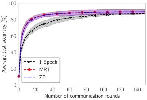
Figure 2: The average test accuracy versus the number of communication rounds for different $\gamma_{k}$ optimization, including no optimization (1 epoch), MRT, and ZF optimization. MRT and ZF greatly outperform the no optimization baseline, showing the importance of an optimization of the local number of iterations based on the solution of problem (18).

Figure 2 shows the average test accuracy versus the number of communication rounds over 10 Monte Carlo iterations using a baseline FedProx with only one epoch, i.e., without $\gamma_{k}$ optimization and using only one SGD iteration. We compare it with the solution of problem (18) by using MRT and ZF beamforming. We assume that $\zeta=1.0$, which means that in each round the devices must harvest all the total energy spent with the training and transmission. Note that the shaded region for the curves represent the standard deviation at each communication round. Without $\gamma_{k}$ optimization, the average test accuracy increases much slower than the MRT and ZF solutions using $\gamma_{k}$ optimization. For instance, at 20 communication rounds the average test accuracy of MRT and ZF are approximately $82\,\mathrm{\%}$, while with one epoch it is only $69\,\mathrm{\%}$. Moreover, there is almost no difference in the average and standard deviation of the test accuracy for MRT and ZF, which is due to a similar number of local iterations from the solution of problem (18). The energy received by ZF is lower than MRT because ZF nulls the interference from neighbouring users, and thus causes inequality (18c) harder to be attainable. To fulfil inequality (18c), the downlink time is increased and the value of $\gamma_{k}$ is decreased, but kept at similar values for both ZF and MRT. Therefore, there are substantial benefits in terms of communication rounds, when optimizing the learning parameters $(\gamma_{k})$ based on the solution of problem (18).

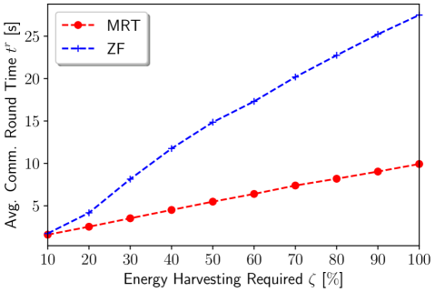
Figure 3: Average time for one communication round $(t^{r})$ versus minimum energy harvesting required $(\zeta)$ with MRT and ZF beamforming. Note that MRT has a much lower communication round time than ZF, which is due to much higher time needed to harvest sufficient energy in the downlink.

Figure 3 shows the average communication round time, $t^{r}$, across all Monte Carlo iterations versus the percentage of energy harvesting required $\zeta$, when using MRT and ZF beamforming. As $\zeta$ increases from $10\,\mathrm{\%}$ to $100\,\mathrm{\%}$, the communication round time increases much faster for ZF than MRT. It indicates that this difference is due to $t_{k}^{d}$ and that inequality (18c), instead of inequality (16c), is the bottleneck for both MRT and ZF. Since ZF nulls the interference from neighbouring users, the total received and harvested power is lower than the MRT case, as expected from the energy harvesting literature [9]. Moreover, it implies that the necessary time to harvest a $\zeta$-percentage of the total energy used by device $k$ is much higher with ZF than MRT. Since MRT and ZF have practically the same test accuracy, the MRT beamforming is a better solution to use in a practical scenario because it provides the best trade-off in terms of test accuracy and energy harvesting capabilities within a short communication round time.

V Conclusion

In this paper, we considered the trade-off between the number of communication rounds in a FL model and the necessary communication round time to harvest energy in an IoT scenario. Specifically, our objective was to minimize the total number of communication rounds necessary to learn a model using FL while minimizing the communication round time, which includes the time to compute and transmit the model, and the time to harvest a sufficient amount of the energy spent during training and transmission. Considering fixed transmit beamforming, this resulted in an optimization problem with learning and time parameters that is jointly convex in all the parameters. The numerical results showed that the solution to this problem using either MRT or ZF beamforming achieves a much higher test accuracy than a baseline solution that does not optimize the learning parameters based on communication aspects. We showed that the MRT beamforming solution provides much lower communication round time than ZF beamforming, while achieving practically the same test accuracy. Therefore, we showed that MRT beamforming is able to achieve a much better trade-off in terms of number of communication rounds and communication round time. For future work, we intend to study the impact of using optimized beamforming and energy harvesting parameters together with the learning and time parameters in the aforementioned trade-off.

Appendix A Proof of Theorem 2

In the following proof, we refer to $h(\mathbf{w}_{k};\mathbf{w}^{t})$ as $h(\mathbf{w}_{k})$, and refer to $\left\|\cdot\right\|_{2}$ as $\left\|\cdot\right\|$ to ease the notation. From [8], recall that the function $h(\mathbf{w}_{k})$ is $\bar{\mu}$-strongly convex, and that the function $F_{k}(\mathbf{w}_{k})$ is $L$-smooth. First, we prove in Lemma 1 that the $h(\mathbf{w}_{k})$ is also $(L+\mu)$-smooth.

Lemma 1.

Consider the function

$$h_{k}(\mathbf{w}_{k})=F_{k}(\mathbf{w}_{k})+\frac{\mu}{2}\left\|\mathbf{w}_{k}-\mathbf{w}^{t}\right\|^{2},$$

where $F_{k}(\mathbf{w}_{k})$ is $L$-smooth. Then, the function $h_{k}(\mathbf{w}_{k})$ is $(L+\mu)$-smooth.

Proof.

Using the definition of $h_{k}(\mathbf{w}_{k})$ for any $\mathbf{w}_{k}$ as $\mathbf{w}$ and $\mathbf{z}$, we have that

$$\nabla^{2}h_{k}(\mathbf{w}) =\nabla^{2}\left(F_{k}(\mathbf{w})+\frac{\mu}{2}\left\|\mathbf{w}-\mathbf{w}^{t}\right\|^{2}\right),$$

$$=\nabla^{2}F_{k}(\mathbf{w})+\mu\mathbf{I},$$

$$\overset{(a)}{\leq}L\mathbf{I}+\mu\mathbf{I}=(L+\mu)\mathbf{I},$$

where $(a)$ is due to $h_{k}(\mathbf{w}_{k})$ being $L$-smooth. Hence, we have proved that the function $h_{k}(\mathbf{w}_{k})$ is $(L+\mu)$-smooth. ∎

Let us assume that $n$ is the last iteration of the local solver using gradient descent, i.e., the inequality $\left\|\nabla h_{k}(\mathbf{w}_{k}^{(n)})\right\|\leq\gamma_{k}^{t}\left\|\nabla h_{k}(\mathbf{w}^{t})\right\|$ is valid with $0\leq\gamma_{k}^{t}\leq 1$. As a local solver, we consider the traditional gradient descent algorithm with step size $\alpha$ and updates as

$$\mathbf{w}_{k}^{(n)}=\mathbf{w}_{k}^{(n-1)}-\alpha\nabla h_{k}(\mathbf{w}_{k}^{(n)}).$$ (19)

We denote as $\mathbf{w}_{k}^{\star}$ the optimal (exact) solution of the optimization problem of minimizing $h_{k}(\mathbf{w}_{k})$ over $\mathbf{w}_{k}$.

Since $h_{k}(\mathbf{w}_{k})$ is $(L+\mu)$-smooth, we have the following inequality between iterations $n$ and $n-1$ [15, Proposition (6.1.2)]:

$$h_{k}(\mathbf{w}_{k}^{(n)}) \leq h_{k}(\mathbf{w}_{k}^{(n-1)})+\nabla{h_{k}(\mathbf{w}_{k}^{(n-1)})}^{\mathrm{T}}\left(\mathbf{w}_{k}^{(n)}-\mathbf{w}_{k}^{(n-1)}\right)+$$

$$\hskip 11.38092pt\frac{L+\mu}{2}\left\|\mathbf{w}_{k}^{(n)}-\mathbf{w}_{k}^{(n-1)}\right\|^{2},$$

$$\overset{(c)}{\leq}h_{k}(\mathbf{w}_{k}^{(n-1)})-\alpha\left\|\nabla h_{k}(\mathbf{w}_{k}^{(n-1)})\right\|^{2}+$$

$$\hskip 11.38092pt\frac{\alpha^{2}(L+\mu)}{2}\left\|\nabla h_{k}(\mathbf{w}_{k}^{(n-1)})\right\|^{2},$$

$$=h_{k}(\mathbf{w}_{k}^{(n-1)})\!-\!\alpha\!\left(\!\frac{2-\alpha(L+\mu)}{2}\!\right)\!\!\left\|\nabla h_{k}(\mathbf{w}_{k}^{(n-1)})\right\|^{2},$$

where $(c)$ is due to Eq. (19).

Hence, we have the following inequality between iterations $n$ and $n-1$:

$$h_{k}(\mathbf{w}_{k}^{(n)})\!\leq h_{k}(\mathbf{w}_{k}^{(n-1)})\!-\!\alpha\left(\!\frac{2-\alpha(L+\mu)}{2}\!\right)\!\left\|\nabla h_{k}(\mathbf{w}_{k}^{(n-1)})\right\|^{2}.$$ (20)

Recall that the function $h_{k}(\mathbf{w}_{k})$ is $\bar{\mu}$-strongly convex. Using the fact that $\nabla h_{k}(\mathbf{w}_{k}^{\star})=\mathbf{0}$, the following inequality holds [15, Eq. (6.20)]:

$$\left\|\nabla h(\mathbf{w}_{k}^{(n-1)})\right\|^{2}\geq\bar{\mu}\left(h_{k}(\mathbf{w}_{k}^{(n-1)})-h_{k}(\mathbf{w}_{k}^{\star})\right).$$

Using the expression above in Eq. (20), we have that:

$$h_{k}(\mathbf{w}_{k}^{(n)}) \leq h_{k}(\mathbf{w}_{k}^{(n-1)})\!-\!\alpha\bar{\mu}\left(\!\frac{2-\alpha(L+\mu)}{2}\!\right)\!\times$$

$$\hskip 11.38092pt\left(h_{k}(\mathbf{w}_{k}^{(n-1)})-h_{k}(\mathbf{w}_{k}^{\star})\right),$$

$$h_{k}(\mathbf{w}_{k}^{(n)})-h_{k}(\mathbf{w}_{k}^{\star}) \overset{(d)}{\leq}\left(h_{k}(\mathbf{w}_{k}^{(n-1)})-h_{k}(\mathbf{w}_{k}^{\star})\right)-$$

$$\hskip 11.38092pt\!\alpha\bar{\mu}\!\left(\!\frac{2-\alpha(L+\mu)}{2}\!\right)\!\!\left(\!h_{k}(\mathbf{w}_{k}^{(n-1)})\!-\!h_{k}(\mathbf{w}_{k}^{\star})\!\right),$$

$$h_{k}(\mathbf{w}_{k}^{(n)})-h_{k}(\mathbf{w}_{k}^{\star}) \overset{(e)}{\leq}\left[1-\!\left(\!\frac{\left(2-\alpha(L+\mu)\right)\alpha\bar{\mu}}{2}\!\right)\right]\times$$

$$\hskip 11.38092pt\left(\!h_{k}(\mathbf{w}_{k}^{(n-1)})\!-\!h_{k}(\mathbf{w}_{k}^{\star})\!\right),$$

$$h_{k}(\mathbf{w}_{k}^{(n)})-h_{k}(\mathbf{w}_{k}^{\star}) \overset{(f)}{\leq}\left[1-\!\left(\!\frac{\left(2-\alpha(L+\mu)\right)\alpha\bar{\mu}}{2}\!\right)\right]^{n}\times$$

$$\hskip 11.38092pt\left(\!h_{k}(\mathbf{w}_{k}^{(0)})\!-\!h_{k}(\mathbf{w}_{k}^{\star})\!\right),$$

$$h_{k}(\mathbf{w}_{k}^{(n)})-h_{k}(\mathbf{w}_{k}^{\star}) \overset{(g)}{\leq}\exp\left[-n\alpha\bar{\mu}\frac{\left(2-\alpha(L+\mu)\right)}{2}\!\right]\times$$

$$\hskip 11.38092pt\left(\!h_{k}(\mathbf{w}_{k}^{(0)})\!-\!h_{k}(\mathbf{w}_{k}^{\star})\!\right),$$ (21)

where $(d)$ adds the term $-h_{k}(\mathbf{w}_{k}^{\star})$ to both sides of the inequality; $(f)$ uses the inequality in $(e)$ in a recursive manner from $n-1$ to $0$; and $(g)$ uses the inequality $(1-x)^{n}\leq\exp(-nx)$.

With Eq. (21), we need to bound the left- and right-hand sides such that we obtain $\gamma_{k}^{t}$. Let us first bound the left-hand side using the $(L+\mu)$-smoothness of $h_{k}(\mathbf{w}_{k})$ at $\mathbf{w}_{k}^{(n)}$ and $\mathbf{w}_{k}^{\star}$ [15, Proposition 6.1.9]:

$$h_{k}(\mathbf{w}_{k}^{(n)}) \geq h_{k}(\mathbf{w}_{k}^{\star})+{\nabla h_{k}(\mathbf{w}_{k}^{\star})}^{\mathrm{T}}\left(\mathbf{w}_{k}^{(n)}-\mathbf{w}_{k}^{\star}\right)+$$

$$\hskip 11.38092pt\frac{1}{2\left(L+\mu\right)}\left\|\nabla h_{k}(\mathbf{w}_{k}^{(n)})-\nabla h_{k}(\mathbf{w}_{k}^{\star})\right\|^{2},$$

$$h_{k}(\mathbf{w}_{k}^{(n)})-h_{k}(\mathbf{w}_{k}^{\star}) \overset{(h)}{\geq}\frac{1}{2\left(L+\mu\right)}\left\|\nabla h_{k}(\mathbf{w}_{k}^{(n)})\right\|^{2},$$ (22)

where $(h)$ uses the fact that $\nabla h_{k}(\mathbf{w}_{k}^{\star})=\mathbf{0}$.

For the right-hand side, we need to use $(L+\mu)$-smoothness [15, Proposition (6.1.2)] at $\mathbf{w}_{k}^{(0)}$ and $\mathbf{w}_{k}^{\star}$:

$$h_{k}(\mathbf{w}_{k}^{(0)}) \leq h_{k}(\mathbf{w}_{k}^{\star})+\nabla h_{k}(\mathbf{w}_{k}^{\star})\left(\mathbf{w}_{k}^{(0)}-\mathbf{w}_{k}^{\star}\right)+$$

$$\hskip 11.38092pt\frac{L+\mu}{2}\left\|\mathbf{w}_{k}^{(0)}-\mathbf{w}_{k}^{\star}\right\|^{2},$$

$$h_{k}(\mathbf{w}_{k}^{(0)})-h_{k}(\mathbf{w}_{k}^{\star}) \overset{(j)}{\leq}\frac{L+\mu}{2}\left\|\mathbf{w}_{k}^{(0)}-\mathbf{w}_{k}^{\star}\right\|^{2},$$ (23)

where $(j)$ uses the fact that $\nabla h_{k}(\mathbf{w}_{k}^{\star})=\mathbf{0}$. Then, we need to use the $\bar{\mu}$-strong convexity of $h_{k}(\mathbf{w})$ [15, Eq. (6.20)] at $\mathbf{w}_{k}^{(0)}$ and $\mathbf{w}_{k}^{\star}$ as follows:

$$\left\|\mathbf{w}_{k}^{(0)}-\mathbf{w}_{k}^{\star}\right\|\leq\frac{1}{\bar{\mu}}\left\|\nabla h_{k}(\mathbf{w}_{k}^{(0)})\right\|.$$ (24)

Combining both Eqs. (23)-(24), we get that:

$$h_{k}(\mathbf{w}_{k}^{(0)})-h_{k}(\mathbf{w}_{k}^{\star}) \leq\frac{L+\mu}{2\bar{\mu}^{2}}\left\|\nabla h_{k}(\mathbf{w}_{k}^{(0)})\right\|^{2},$$

$$h_{k}(\mathbf{w}_{k}^{(0)})-h_{k}(\mathbf{w}_{k}^{\star}) \overset{(k)}{\leq}\frac{L+\mu}{2\bar{\mu}^{2}}\left\|\nabla F_{k}(\mathbf{w}^{t})\right\|^{2},$$ (25)

where $(k)$ uses the assumption that $\mathbf{w}_{k}^{(0)}=\mathbf{w}^{t}$.

Using the bounds for left-hand side in Eq. (22) and for the right-hand side in Eq. (25) of Eq. (21), we have that:

$$\frac{1}{2\left(L+\mu\right)}\left\|\nabla h_{k}(\mathbf{w}_{k}^{(n)})\right\|^{2} \leq\exp\left[-n\alpha\bar{\mu}\frac{\left(2-\alpha(L+\mu)\right)}{2}\!\right]\times$$

$$\hskip 11.38092pt\frac{L+\mu}{2\bar{\mu}^{2}}\left\|\nabla F_{k}(\mathbf{w}^{t})\right\|^{2},$$

$$\left\|\nabla h_{k}(\mathbf{w}_{k}^{(n)})\right\|^{2} \overset{(l)}{\leq}\left(\!\!\left(\frac{L+\mu}{\bar{\mu}}\right)\exp\left(\frac{-n}{2\beta}\!\right)\!\!\right)^{2}\!\!\times$$

$$\hskip 11.38092pt\left\|\nabla F_{k}(\mathbf{w}^{t})\right\|^{2}\!\!,$$ (26)

where $(l)$ reorganizes the terms with the definition of $\beta\!=\!\tfrac{2}{\alpha\bar{\mu}\left(2-\alpha(L+\mu)\right)}$, with $\alpha\!<\!\tfrac{2}{L+\mu}$. To ensure a $\gamma_{k}^{t}$-inexact solution as in Definition 1, and using Eq. (26), we need to ensure that:

$$\left(\frac{L+\mu}{\bar{\mu}}\right)\exp\left(\frac{-n}{2\beta}\!\right)\leq\gamma_{k}^{t}.$$

If we reorganize the inequality above, we have that:

$$\exp\left(\frac{-n}{2\beta}\!\right) \leq\frac{\gamma_{k}^{t}\bar{\mu}}{L+\mu},$$

$$\frac{-n}{2\beta} \overset{(m)}{\leq}\log\left(\frac{\gamma_{k}^{t}\bar{\mu}}{L+\mu}\right),$$

$$n \overset{(o)}{\geq}2\beta\log\left(\frac{L+\mu}{\gamma_{k}^{t}\bar{\mu}}\right),$$ (27)

$(m)$ applies the logarithm function on both sides of the inequality; and $(o)$ reorganizes the term in the logarithmic function such that the sign on both sides of the inequality is reordered. By redefining $n$ as $I_{k}$, we have proved the bound of the number of iterations proposed in Theorem 2.

References

- [1] Ericsson, “Ericsson mobility report,” Ericsson AB, Tech. Rep., Nov. 2020. [Online]. Available: https://bit.ly/32jKqGg
- [2] Z. Zhou, X. Chen, E. Li, L. Zeng, K. Luo, and J. Zhang, “Edge Intelligence: Paving the Last Mile of Artificial Intelligence With Edge Computing,” Proceedings of the IEEE, vol. 107, no. 8, pp. 1738–1762, Aug. 2019.
- [3] H. B. McMahan, E. Moore, D. Ramage, S. Hampson, and B. A. y Arcas, “Communication-efficient learning of deep networks from decentralized data,” in International Conference on Artificial Intelligence and Statistics, 2017, pp. 1273–1282.
- [4] H. Hellström, J. M. B. da Silva Jr., V. Fodor, and C. Fischione, “Wireless for Machine Learning,” arXiv preprint arXiv:2008.13492, Sep. 2020.
- [5] B. Clerckx, K. Huang, L. R. Varshney, S. Ulukus, and M.-S. Alouini, “Wireless Power Transfer for Future Networks: Signal Processing, Machine Learning, Computing, and Sensing,” arXiv preprint arXiv:2101.04810, 2021.
- [6] B. Clerckx, R. Zhang, R. Schober, D. W. K. Ng, D. I. Kim, and H. V. Poor, “Fundamentals of Wireless Information and Power Transfer: From RF Energy Harvester Models to Signal and System Designs,” IEEE Journal on Selected Areas in Communications, vol. 37, no. 1, pp. 4–33, Jan. 2019.
- [7] Q. Zeng, Y. Du, and K. Huang, “Wirelessly Powered Federated Edge Learning: Optimal Tradeoffs Between Convergence and Power Transfer,” arXiv preprint arXiv:2102.12357, 2021.
- [8] T. Li, A. K. Sahu, M. Zaheer, M. Sanjabi, A. Talwalkar, and V. Smith, “Federated Optimization in Heterogeneous Networks,” in Proceedings of Machine Learning and Systems, 2020, pp. 429–450.
- [9] S. Timotheou, I. Krikidis, G. Zheng, and B. Ottersten, “Beamforming for MISO Interference Channels with QoS and RF Energy Transfer,” IEEE Transactions on Wireless Communications, vol. 13, no. 5, pp. 2646–2658, May 2014.
- [10] Z. Yang, M. Chen, W. Saad, C. S. Hong, and M. Shikh-Bahaei, “Energy Efficient Federated Learning Over Wireless Communication Networks,” IEEE Transactions on Wireless Communications, vol. 20, no. 3, pp. 1935–1949, Mar. 2021.
- [11] X. Xu, A. Özçelikkale, T. McKelvey, and M. Viberg, “Simultaneous Information and Power Transfer under a Non-Linear RF Energy Harvesting Model,” in IEEE International Conference on Communications Workshops (ICC Workshops), 2017, pp. 179–184.
- [12] S. Diamond and S. Boyd, “CVXPY: A Python-embedded modeling language for convex optimization,” Journal of Machine Learning Research, vol. 17, no. 83, pp. 1–5, 2016.
- [13] P. Gahinet, A. Nemirovski, A. J. Laub, and M. Chilali, “LMI Control Toolbox User’s Guide,” Mathworks, Natick, MA, USA, Tech. Rep., 1995.
- [14] 3GPP, “Evolved Universal Terrestrial Radio Access (E-UTRA); Further enhancements to LTE Time Division Duplex (TDD) for Downlink-Uplink (DL-UL) interference management and traffic adaptation,” 3rd Generation Partnership Project (3GPP), TR 36.828, Jun. 2012.
- [15] D. P. Bertsekas, Convex Optimization Algorithms. Athena Scientific, 2015.