Abstract

In the quantum models described by analytic potentials $V(r)$ with several pronounced minima the phenomenon of tunneling opens the possibility of a sudden relocalization of the system after a minor modification of parameters. This may really reorder the minima and change, thoroughly, the shape of the (measurable) probability density. In the spectrum one observes the “avoided crossings” of the energy levels. By definition, the relocalization configurations are sensitive to perturbations and represent, therefore, a crossroad to alternative evolution scenarios. As long as the numerical search for these quantum analogues of the Thom’s classical catastrophes is not easy, a systematic non-numerical approach is proposed here, based on an exact (or, better, quasi-exact) simultaneous construction of mutually consistent pairs of potentials $V(r)$ and wave functions $\psi(r)$.

keywords

partially solvable quantum models; potentials with multiple minima; relocalizations of probability densities;

1 Introduction

One-dimensional Schrödinger equation

$$\left[-\frac{d^{2}}{d{r}^{2}}+V({r})\right]\,\psi({r})=E\,\psi({r})\,,\ \ \ \ \psi({r})\in L^{2}(\mathbb{R})\,$$ (1)

often serves as a methodical laboratory and testing ground guiding the analysis of various more sophisticated (e.g., higher-dimensional or multi-particle) models of the physical reality studied on the level of microworld. Sometimes, it is being forgotten that even the drastically simplified quantum model (1) can also represent a system of its own, immediate physical interest.

In our present paper the latter idea is to be supported by the turn of attention to the less elementary forms of potentials $V(r)$ characterized by the presence of several pronounced and deep, more or less independent local minima separated by non-negligible barriers of a variable thickness. In this sense our present study was inspired by our recent paper [1] in which we revealed that in spite of an apparently purely numerical character of any explicit construction of predictions provided by a class of general polynomial potentials, there exist several well formulated problems (inspired by the classical Thom’s theory of catastrophes [2]) in which the predictions of certain experimentally relevant “quantum catastrophes” could still be based on the use of certain non-numerical approximation techniques.

In what follows a continuation of the latter project will be developed in two directions. First, in the context of mathematics we shall advocate the tractability of Eq. (1) even when potentials $V(r)$ possess certain non-polynomial forms. Second, in the above-mentioned context of physics of catastrophes modeled in a genuine quantum meaning of the word, we shall propose and develop an innovative approach in which one relocates, in some sense, the role of an input dynamical information about the system from $V(r)$ to a particular $\psi(r)$.

In section 2 we will outline the basic physical motivation of such a project. We will explain the phenomenological as well as theoretical usefulness of the specific experiment-related concept of the so called avoided level crossing (ALC). This outline of motivation will continue in section 3 explaining the merits of our proposal of analysis of the ALC-related physics using the mathematical methods of construction of the so called quasi-exactly solvable (QES) quantum models.

In section 4 we will briefly formulate our methodical message connecting the exciting physical relevance of the deep multi-valley potentials with an optimality of the description of bound states using the QES techniques. The technical core of our paper is then developed in section 5. Via a detailed analysis of the QES models with three or four almost separate deep-valley subsystems we deduce and support our main observation that even a comparatively simple version of the QES philosophy offers a particularly fortunate interplay between a desirable flexibility of the picture of physics and a user-friendliness of its mathematical representation using non-polynomial but still elementary and analytic forms of potentials.

Section 6 is then devoted to the analysis of some specific consequences of the tunneling through multiple barriers and to the related approximate degeneracy of multiple low-lying states. We will point out, in particular, that in such an arrangement one has to deal with a very specific form of the conventional oscillation theorems. In subsequent section 7 we also turn attention to a broader context of multiple-well models and to their possible future role in the quantum theory of catastrophes involving more than just the relocalizations of ground states.

Section 8 is summary.

2 Avoided level crossings

The ubiquitous quantum phenomenon of avoided level crossings (ALC) finds one of its most straightforward illustrations in the one-dimensional bound-state problem (1) with a highly schematic rectangular double-well potential

$$V(r)=V^{(RDW)}(r,a,b,c)=\left\{\begin{array}[]{ll}\infty\,,&r\in(-\infty,-3)\\ a^{2}\,,&r\in(-3,-1)\\ b^{2}\,,&r\in(-1,1)\\ c^{2}\,,&r\in(1,3)\\ \infty\,,&r\in(3,\infty)\,.\end{array}\right.$$ (2)

In the case of a high central barrier, $b^{2}\gg\max(a^{2},c^{2})$, the low-lying spectrum of energies $E_{n}$ with $n=0,1,\ldots,N_{\max}$ can be perceived as composed of the two practically independent left-well and right-well low-lying approximate subspectra

$$E_{p}^{\rm(left)}=a^{2}+\left[k_{p}^{\rm(left)}\right]^{2}\,,\ \ \ \ k_{p}^{\rm(left)}=(p+1)\,\pi/2\,,\ \ p=0,1,\ldots,P_{\max}\,$$ (3)

and

$$E_{q}^{\rm(right)}=c^{2}+\left[k_{q}^{\rm(right)}\right]^{2}\,,\ \ \ \ k_{q}^{\rm(right)}=(q+1)\,\pi/2\,,\ \ q=0,1,\ldots,Q_{\max}\,.$$ (4)

In such an extreme dynamical regime the wave functions will contain the well known [3] single-well components $\psi_{n_{1}}^{\rm(left)}(r)$ and $\psi_{n_{2}}^{\rm(right)}(r)$,

$$\psi_{(n_{1},n_{2})}(r)=\left\{\begin{array}[]{ll}0\,,&r\in(-\infty,-3)\\ \psi_{n_{1}}^{\rm(left)}(r)+{\rm small\ corrections}\,,&r\in(-3,-1)\\ 0+{\rm small\ corrections}\,,&r\in(-1,1)\\ \psi_{n_{2}}^{\rm(right)}(r)+{\rm small\ corrections}\,,&r\in(1,3)\\ 0\,,&r\in(3,\infty)\,.\end{array}\right.$$ (5)

In particular, for the ground state with approximate energy $E_{0}(a,c)=\min(E_{0}^{\rm(left)},E_{0}^{\rm(right)})=\min(a^{2},c^{2})+\pi^{2}/4$, we will have $\psi_{0}^{\rm(left/right)}(r)\sim-\cos k_{0}^{\rm(left/right)}r$ with $k_{0}^{\rm(left)}=\sqrt{E_{0}-a^{2}}$ and $k_{0}^{\rm(right)}=\sqrt{E_{0}-c^{2}}$. In the generic cases the subdominant component will be strongly suppressed (i.e., $\psi_{0}^{\rm(right)}(r)$ will lie too high at $a^{2}\ll c^{2}$, and vice versa). The related local suppressions of the probability density will be an observable effect.

In the non-generic limit of $a^{2}\approx c^{2}$, the ALC effect will occur. The approximate coincidence of the left-well and right-well subspectra will be accompanied by the approximate degeneracy of the first two lowest energies, $E_{0}\lessapprox E_{1}$. The suppression of the subdominant component of the wave function will temporarily disappear. Due to the process of an ALC-related instantaneous exchange of dominance of the two subsystems, the ground- and the first excited state will form a doublet characterized by different parities but practically the same probability density, $\psi^{*}_{1}(x)\psi_{1}(x)\approx\psi^{*}_{0}(x)\psi_{0}(x)$.

In our preceding paper [1] we pointed out that the price paid for the exact solvability of the rectangular double- and multi-well models as sampled by Eq. (2) is too high. In any sufficiently realistic experimental setup the shape of the potential is certainly different: smooth and non-rectangular. The more realistic polynomial potential may still lead to a satisfactory approximate solvability of the related Schrödinger equation. Moreover, the polynomiality of potentials admits an analytic continuation of the model. This is a useful mathematical trick which can relate the ALC-accompanying attraction/repulsion of energies to a proximity of the so called Kato’s exceptional-point (EP, [4]) in the complex plane of a suitable parameter [5].

For all of these reasons we proposed, in [1], that the study of the ALC effects might find a suitable benchmark-model background in analytic Arnold-inspired polynomial potentials $V_{(Arnold)}(r)$. This resulted in an amendment of our understanding of some ALC-related phenomena [6]. In parallel, an important weakness of the innovation may be seen in a retreat from the exact solvability of the rectangular-well models to the mere approximate forms of the solutions, i.e., of the verifiable and measurable predictions. This was a challenge which led to a modification of the model-building strategy. Its form will be described and illustrated in what follows.

3 Conventional QES constructions

3.1 The change of paradigm

The birth of the concept of quasi-exactly solvable (QES) Schrödinger equations (see the compact review of its various aspects and, in particular, Appendix A in Ushveridze’s monograph [7]) contributed to an enhancement of efficiency of several model-building strategies in quantum mechanics. In the narrower context of Eq. (1) the essence of amendment lies in a modification of the conventional textbook philosophy in which a “known” potential $V(r)$ is given in advance while the “unknown” bound states $\psi(r)$ must be reconstructed via ordinary differential Schrödinger Eq. (1) [3]. On this background the QES-based model-building strategy is more balanced, transferring a part of the technical simplicity assumptions from $V(r)$ to $\psi(r)$.

In our present application of the QES model-building strategy we decided to rewrite the above-mentioned Schrödinger equation into its formally equivalent form of definition of a QES-compatible potential,

$$V_{(QES)}({r})=E_{(QES)}+\psi^{\prime\prime}_{(QES)}({r})/\psi_{(QES)}({r})\,.$$ (6)

In such an extreme version of the QES approach one interchanges the roles of $V(r)$ and $\psi(r)$, and one inverts the conventional construction completely. The duty of the carrier of the physical input information is fully transferred from $V(r)$ to an ansatz for a QES state $\psi(r)=\psi_{(QES)}({r})$.

Our recommendation of replacement of Eq. (1) by Eq. (6) found its immediate encouragement in the emergence of certain descriptive shortcomings of the poolynomial-interaction models as used in [1]. A family of Schrödinger Eqs. (1) has been considered there in a specific dynamical regime controlled by potentials with pronounced multiple minima. In this regime the phenomenologically most interesting feature of the system has been found to lie in the possibility of a sudden change of the topological structure of the probability densities. We revealed that in general, these changes (called, “quantum relocalization catastrophes”) appeared caused by certain very small changes of some parameters in the potential.

In [1], unfortunately, the conventional insistence on the elementary form (viz., just polynomial form) of the potentials implied that we could only work with certain approximate forms of the wave functions. The sensitivity of the observable catastrophic effects to the physical parameters interfered with the influence of the round-off errors in $\psi(r)$. This was a serious drawback and weakness of the method. In our present paper we will show that the unavoidable enhancement of the precision of wave functions can in fact be easily achieved via the less conventional QES approach. In its framework, the original difficult search for the instants of the relocalization catastrophes based on the brute-force solution of Eq. (1) will drastically be simplified.

We should add that the QES-based change of perspective is in fact much less revolutionary than it may seem to be. Indeed, from a strictly local point of view the difference between “the old exact input” $V_{(Arnold)}(r)$ and “the new exact input” $\psi_{(QES)}(r)$ only becomes visible on the level of corrections. In particular, potentials $V_{(Arnold)}(r)$ and $V_{(QES)}(r)$ are both  fairly well approximated, near their deep minima, by the conventional and exactly solvable harmonic-oscillator wells. For this reason, also the local forms of the related ground-state wave functions $\psi_{(QES)}(r)$ and $\psi_{(Arnold)}(r)$ are both well approximated by the Gaussians.

3.2 An illustrative sextic-anharmonic-oscillator example

In the extensive dedicated literature (cited, e.g., in [7]) interested readers could find several other, less elementary examples and generalizations of the QES idea and constructions. Some of them possess an intriguing mathematical background [8] while some other put more emphasis upon nontrivial phenomenological applications [9]. Thus, for example, the most recent studies are revealing new links between the QES models and the theory of special functions [10]. These samples of the technical and mathematical progress are also currently accompanied by the innovative phenomenological applications of the various multi-well-shaped potentials, say, in nuclear physics [11]. For our present purposes, incidentally, we will only need the technically less sophisticated version of the recipe. In the overall QES context the input information represented exclusively by the potential will be considered here an expensive luxury. A compensation will be sought in a more balanced model-building strategy.

One of the best known and probably also one of the oldest illustrations of such an attitude is provided by the sextic-polynomial interaction potential [10, 11, 12]

$$V({r})=A\,{r}^{2}+B\,{r}^{4}+{r}^{6}\,.$$ (7)

Its insertion in Eq. (1) would only lead to a purely numerical problem in general. In the QES setting, therefore, the overall two-parametric definition (7) is to be simplified and accompanied by an additional requirement that the underlying Schrödinger equation should generate at least one wave function which is exact and elementary. Once such a function is prescribed, say, in the simplest possible one-parametric single-exponential ground-state form

$$\psi_{(QES)}({r})=\exp\left[-\frac{1}{4}({r}^{2}+\alpha)^{2}\right]\,$$ (8)

it is still possible to guarantee that our Schrödinger Eq. (1) will be satisfied. Indeed, it is an entirely elementary exercise to verify that for the specific QES ansatz (8) it is sufficient to reparametrize, self-consistently, the energy $E=\alpha$ in Eq. (1) as well as the couplings $A=A(\alpha)=\alpha^{2}-3\,$ and $B=B(\alpha)=2\alpha$ in Eq. (7).

Besides the methodical appeal of ansatz (8) also the related picture of dynamics is remarkable. The QES version of potential (7) acquires the single-well shape at $\alpha>\sqrt{3}$, the double-well shape at $-\sqrt{3}<\alpha<\sqrt{3}$, and the triple-well shape at $\alpha<-\sqrt{3}$. Unfortunately, the variability of the shape of $V({r})$ is only partially paralleled by the flexibility of the measurable probability density $\varrho(x)=\psi^{*}(x)\psi(x)$ possessing just two maxima at most.

The latter observation gave birth to our present study. In essence, a phenomenologically richer menu of bound states will be obtained via a multi-term extension of the class of the QES ansatzs as sampled by Eq. (8).

4 Relocalization catastrophes

In the theory of classical dynamical systems the concept of equilibrium can be given a neat geometric interpretation [2]. The related mathematics also offers a systematic classification of the processes during which these equilibria are being lost or established [13]. These considerations were made particularly popular by René Thom [14] who selected seven most elementary transmutations of the classical equilibria and gave them specific nicknames like “cusp”, etc.

Whenever one tries to extend the Thom’s systematics to the theory of quantum dynamical systems one must imagine that in quantum dynamical systems the predictions of any measurable effect become merely probabilistic, based on Schrödinger equation.

4.1 Polynomial multi-barrier potentials

In a way inspired by the Arnold’s treatment of the classical  catastrophe theory [13]) we considered, in our recent paper [1], all of the confining and spatially-symmetric polynomial quantum potentials

$$V_{(Arnold)}(r)=x^{2N+2}+c_{1}\,r^{2N}+c_{2}\,r^{2N-2}+\ldots+c_{N}\,r^{2}\,,\ \ \ \ r\in(-\infty,\infty).$$ (9)

We restricted our attention to the multi-well dynamical regime in which the potential developed an $N-$plet of high and thick barriers. Near a pronounced and dominant minimum of the potential (i.e., say, at $r\approx a$ such that $V^{\prime}_{(Arnold)}(a)=0$) the ground state energy proves well approximated by the leading-order formula

$$E_{0}\approx V_{(Arnold)}(a)+\omega^{(\min)}\,,\ \ \ \ \omega^{(\min)}=V^{\prime\prime}_{(Arnold)}(a)/2\,.$$ (10)

Naturally, under an additional, ad hoc  assumption of the left-right symmetry of the Arnold’s potential (9) we have to keep in mind that unless $a=0$ these global minima occur in pairs. This means that the approximate form of the generic ground-state wave function will have two components at $a\neq 0$,

$$\psi^{(Arnold)}(r)\sim\exp[-\omega^{(\min)}(r-a)^{2}]+\exp[-\omega^{(\min)}(r+a)^{2}]\,$$ (11)

Even if the anharmonic corrections to the generic formula (11) remain negligible one should take into consideration also all of the non-generic situations in which the nontrivial contributions to $\psi^{(Arnold)}(r)$ come from the broader subdominant local minima $r=\pm a_{j}$ of the potential satisfying the condition of coincidence of the leading-order ground-state energies,

$$E=E_{0}(j)=V_{(Arnold)}(a_{j})+\omega^{(\min)}_{j}=E(M)\,,\ \ \ \ j=1,2,\ldots,M\,.$$ (12)

In this setting the reliability of the leading-order approximation must be based not only on a guarantee of the sufficiently large size of all of the constants $\omega^{(\min)}_{j}$ with $j=1,2,\ldots,M$ (making the first local excitations $E_{1}(j)=E_{0}(j)+2\,\omega^{(\min)}_{j}$ sufficiently well separated) but, first of all, on a sufficiently strong suppression of the potential influence of the ground-state contributions coming from all of the other potentially eligible local minima,

$$E_{0}(k)=V_{(Arnold)}(a_{k})+\omega^{(\min)}_{k}\gg E(M)\,,\ \ \ \ k=M+1,M+2,\ldots,N+1\,.$$ (13)

In such a case the leading-order ground-state wave functions will have the form of superpositions

$$\psi^{(Arnold)}_{0}(r)\sim\sum_{j=1}^{M}\,p_{j}\,\left[\exp[-\omega^{(\min)}_{j}(r-a_{j})^{2}]+\exp[-\omega^{(\min)}_{j}(r+a_{j})^{2}]\right]\,.$$ (14)

In [1] it has been emphasized that the latter solutions will be highly sensitive to certain very small changes of parameters $c_{k}$ in potentials (9). Such a change will cause, typically, a relocation of a subset of the $M-$plet of the initial local minima from the dominant category (12) to the subdominant category (13). In Eq. (14), due to the tunneling, the respective coefficients $p_{j}$ will then vanish. For this reason also the related probability density $\varrho(x)=\psi^{*}(x)\psi(x)$ will change accordingly. The process (during which the value of $M$ decreased) can be also inverted (leading to an increase of the number $M$ of participating local minima). Finally, a combination of the two processes (initiated and ending, in long run, at the two different and stable equilibria with $M=1$) has been given, in [1], the name of a relocalization quantum catastrophe. In this context, our present main ambition may be briefly characterized as a QES-based closed-form description of the relocalization-catastrophe instants with an arbitrarily large degree of the instantaneous degeneracy $M>1$.

4.2 Double-well Gaussian ansatz

In a certain parallel to the above-outlined non-smooth model (2) let us now contemplate the smooth and most elementary pair-of-oscillators ansatz

$$\psi^{(2)}(r)=\exp[-(r-a)^{2}]+\exp[-(r+a)^{2}]\,.$$

At a large separation parameter $a\gg 1$ it represents, locally, two independent harmonic oscillators in ground state. Such an asymptotically elementary formula offers a perfect insight in the shape of the wave function but as a starting point of reconstruction of a related potential it looks clumsy and can be simplified,

$$\psi^{(2)}(r)=2\,\exp(-r^{2}-a^{2})\,{\rm cosh}\,(2ar)\,.$$ (15)

This function is better suited for insertion in formula (6) yielding

$$V({r})=E+\psi^{\prime\prime}(r)/\psi(r)=E-2+{4a^{2}}+4\,r^{2}-8\,ar\,{{\rm tanh}\,(2ar)}\,.$$

As long as the anharmonicity remains asymptotically subdominant we may immediately conclude that the high excitations will feel it as a not too essential perturbation. The situation becomes different for the low-lying bound states because the potential acquires, near the origin, the double-well shape at $a^{2}>1/4$. Once we set, say, $V(0)=0$, the explicit ground-state QES energy value becomes equal to $E_{0}=2-{4a^{2}}$. Its value decreases with the growth of $a^{2}$ and it drops below the local maximum of the potential at $a^{2}=1/2$. Subsequently, the potential acquires the clear double-well shape. At the sufficiently large $a\gg 1$ we get $V(r)\approx 4\,r^{2}-8\,a|r|$, i.e., $V(r)\approx 4\,(r-a)^{2}-4\,a^{2}$ at the positive $r\gg 1$, and $V(r)\approx 4\,(r+a)^{2}-4\,a^{2}$ at the negative $r\ll-1$. The minima at $r\approx\pm a$ are deep so that with good precision the low-lying spectrum becomes tractable as a well-separated pair of the two remote harmonic oscillators.

A generalization of this observation will be slightly more complicated but straightforward.

5 Multi-Gaussian models

The QES approach based on Eq. (6) makes it clear that the conventional constraints of the polynomiality of $V(r)$ limit the variability of the shapes of the wave functions $\psi(r)$. In [1], the necessarily non-exact, approximate forms of the wave function solutions led also to the mere approximate form of the predictions of the measurable effects. Another technical obstruction consisting in the non-geometric, deeply quantum nature of the relocalization catastrophes has been also circumvented using suitable approximations of the energies as sampled by formula (10) above.

In this sense we were only able to rely on approximate results. In the present paper, in contrast, we will insist on the exact QES form of the wave functions. This will enable us to move to the more complicated QES ansatzs and, ultimately, to oppose, constructively, the not too deeply motivated traditional restriction of the form of the dynamical input information to the mere polynomial class of the potentials.

5.1 Three equidistant Gaussians

The $M=3$ QES ansatz

$$\psi^{(3)}(r)=\exp[-(r-b)^{2}]+\exp(-r^{2})+\exp[-(r+b)^{2}]$$

can be simplified,

$$\psi^{(3)}(r)=\exp(-r^{2})[1+2\,e^{-b^{2}}{\rm cosh}\,(2br)]$$ (16)

and factorized,

$$\psi(r)={e^{-{r}^{2}}}\,F({}\,r)\,.$$

On this ground we easily evaluate

$$\psi^{\prime}(r)=-2\,r\,\psi+{e^{-{r}^{2}}}\,F^{\prime}({}\,r)$$

and

$$\psi^{\prime\prime}(r)=(4\,r^{2}-2)\,\psi-4\,r\,{e^{-{r}^{2}}}\,F^{\prime}({}\,r)+{e^{-{r}^{2}}}\,F^{\prime\prime}({}\,r)$$

so that, finally,

$$V({r})=E+\psi^{\prime\prime}(r)/\psi(r)=E-2+4\,r^{2}-4\,r\,\frac{F^{\prime}({}\,r)}{F({}\,r)}+\frac{F^{\prime\prime}({}\,r)}{F({}\,r)}\,.$$ (17)

Although such a QES potential is not a polynomial, its form remains elementary in general. In particular, at $M=3$ we have

$$F(r)=1+2\,e^{-b^{2}}{\rm cosh}\,(2br)$$

so that

$$F^{\prime}(r)=4b\,e^{-b^{2}}{\rm sinh}\,(2br)$$

with

$$F^{\prime}(r)/F(r)=\frac{4b\,e^{-b^{2}}{\rm sinh}\,(2br)}{1+2\,e^{-b^{2}}{\rm cosh}\,(2br)}$$

and with

$$F^{\prime\prime}(r)=8b^{2}\,e^{-b^{2}}{\rm cosh}\,(2br)$$

in

$$F^{\prime\prime}(r)/F(r)=\frac{b^{2}\,(8e^{-b^{2}}{\rm cosh}\,(2br)+4-4)}{1+2\,e^{-b^{2}}{\rm cosh}\,(2br)}=4b^{2}-\frac{4b^{2}\,}{1+2\,e^{-b^{2}}{\rm cosh}\,(2br)}\,.$$

This yields the potential

$$V(r)-E_{0}=-2+4\,b^{2}+4r^{2}+A/B\,,\ \ \ \$$ (18)

where

$$A={{-16\,br\sinh\left(2\,br\right){e^{-{b}^{2}}}-4\,b^{2}}}\,,\ \ \ \ B={2\,\cosh\left(2\,br\right){e^{-{b}^{2}}}+1}\,.$$

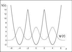
Figure 1: The choice of a sufficiently large shift in the QES ansatz (16) (here, $b=4$) keeps the barriers sufficiently thick to suppress the tunneling between the three deep wells (in our units, the display of the QES input wave function is six times enlarged).

Although the latter algebraic presentation of the resulting QES potential is exact, it is both unusual and rather counterintuitive. Its better perception can easily be obtained when we choose any sufficiently large value of the parameter (say, $b=4$) and draw a picture (see Fig. 1). Its inspection immediately reveals that the shape of potential (18) is in fact just a chain of four independent wells of an approximately harmonic-oscillator form.

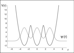
Figure 2: A perceivable thinning of the barriers followed by an enhancement of the tunneling occurs at an intermediate shift $b=3$ in the QES ansatz (16).

Once we choose a smaller but still sufficiently large value of $b=3$, the overall picture does not change too much (see Fig. 2). Only after we further move to the still smaller value of $b=2$ (see Fig. 3), we discover what happens when the overlaps between the Gaussians become large. At a still smaller $b=\sqrt{2}$ the wave function itself even ceases to possess the local minima although the triple-well structure of the potential still survives. At $b=1$ one only finds a not too pronounced double-well shape of $V(r)$, and there are no traces of the shift left in the potential at $b=1/2$.

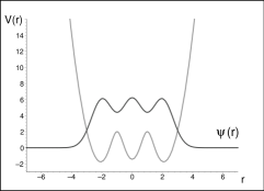
Figure 3: At the small shift $b=2$ in (16) the barriers are too low to suppress the tunneling.

All of the expectations based on the pictures may be complemented by the easy but rigorous Taylor-series expansions of the potential at any relevant coordinate of interest. For example, in the vicinity of the origin we get, at an arbitrary parameter $b$, formula

$$V(r)-E=2\,{\frac{4\,{b}^{2}{e^{-{b}^{2}}}-2\,{e^{-{b}^{2}}}-1}{2\,{e^{-{b}^{2}}}+1}}+$$

$$+4\,{\frac{-16\,{b}^{2}{e^{-2\,{b}^{2}}}-8\,{b}^{2}{e^{-{b}^{2}}}+4\,{e^{-2\,{b}^{2}}}+4\,{e^{-{b}^{2}}}+1+4\,{b}^{4}{e^{-{b}^{2}}}}{\left(2\,{e^{-{b}^{2}}}+1\right)^{2}}}{r}^{2}-$$

$$-16/3\,{\frac{{b}^{4}{e^{-{b}^{2}}}\left(-32\,{e^{-2\,{b}^{2}}}-8\,{e^{-{b}^{2}}}+4+10\,{b}^{2}{e^{-{b}^{2}}}-{b}^{2}\right)}{\left(2\,{e^{-{b}^{2}}}+1\right)^{3}}}{r}^{4}+O\left({r}^{6}\right)\,,$$

etc. For comparison, we can expand the wave function,

$$\psi(r)=(2\,{e^{-{b}^{2}}}+1+\left(4\,{b}^{2}{e^{-{b}^{2}}}-2\,{e^{-{b}^{2}}}-1\right){r}^{2}+\left(4/3\,{b}^{4}{e^{-{b}^{2}}}+{e^{-{b}^{2}}}+{\frac{1}{2}}-4\,{b}^{2}{e^{-{b}^{2}}}\right){r}^{4}+O\left({r}^{6}\right))$$

and also its derivative,

$$\psi^{\prime}(r)=\left(8\,{b}^{2}{e^{-{b}^{2}}}-4\,{e^{-{b}^{2}}}-2\right)r+\left(-16\,{b}^{2}{e^{-{b}^{2}}}+4\,{e^{-{b}^{2}}}+2+16/3\,{b}^{4}{e^{-{b}^{2}}}\right){r}^{3}+$$

$$+\left(-8\,{b}^{4}{e^{-{b}^{2}}}-2\,{e^{-{b}^{2}}}-1+12\,{b}^{2}{e^{-{b}^{2}}}+{\frac{16}{15}}\,{b}^{6}{e^{-{a}^{2}}}\right){r}^{5}+O\left({r}^{6}\right)\,$$

serving, e.g., the purposes of a more detailed analysis.

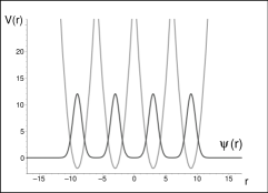
Figure 4: At the value of $a=3$ in (19) the three barriers prove thick enough to suppress the tunneling.

5.2 Four equidistant Gaussians

Once we wish to reconfirm the above picture- and intuition-based messages we may just repeat the construction at $M=4$, with the QES ansatz

$$\psi^{(4)}(r)=\exp[-(r-3\,a)^{2}]+\exp[-(r-a)^{2}]+\exp[-(r+a)^{2}]+\exp[-(r+3\,a)^{2}]$$

abbreviated as

$$\psi^{(4)}(r)=2\,\exp(-r^{2}-a^{2})\,[{\rm cosh}\,(2ar)+e^{-8a^{2}}{\rm cosh}\,(6ar)]$$

and yielding

$$F(r)={\rm cosh}\,(2ar)+e^{-8a^{2}}{\rm cosh}\,(6ar)\,,$$

$$F^{\prime}(r)=2a\,{\rm sinh}\,(2ar)+6a\,e^{-8a^{2}}{\rm sinh}\,(6ar)\,$$

and

$$F^{\prime\prime}(r)=4a^{2}\,{\rm cosh}\,(2ar)+36\,a^{2}\,e^{-8a^{2}}{\rm cosh}\,(6ar)\,.$$

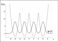
Figure 5: For ansatz (19) the lowering of the barriers and the first marks of the tunneling emerge at $a=2$.

The existence of the quadruplet of the coordinates $-3a,-a,a,3a$ approximating the local minima of $V(r)$ could again be shown to lead to the analogous graphical results at $a=3$ (see Fig. 4) and at $a=2$ (see Fig. 5). In the latter picture with $a=2$ we see again an onset of the tunneling which becomes detected but remains weak. In contrast, at $a=1$ one would already get a strong tunneling supporting a four-bump analogue of the three-bump structures as depicted in Fig. 3 above. With the further decrease of $a$ the wave functions and, slightly later, also the potentials would lose again their local minima and maxima. Only the potential themselves still exhibit, even at a very small shift $a=1/2$, the very week remnants of their last two minima.

In the language of algebra with

$$\psi(r)={e^{-{r}^{2}}}\left(2\,\cosh\left(2\,ar\right){e^{-{a}^{2}}}+2\,\cosh\left(6\,ar\right){e^{-9\,{a}^{2}}}\right)$$ (19)

we get the numerator of the potential in the form

$$4\,{e^{-{a}^{2}-{r}^{2}}}(-\cosh\left(2\,ar\right)-\cosh\left(6\,ar\right){e^{-8\,{a}^{2}}}+2\,{r}^{2}\cosh\left(2\,ar\right)+2\,{r}^{2}\cosh\left(6\,ar\right){e^{-8\,{a}^{2}}}-$$

$$-4\,r\sinh\left(2\,ar\right)a-12\,r\sinh\left(6\,ar\right)a{e^{-8\,{a}^{2}}}+2\,\cosh\left(2\,ar\right){a}^{2}+18\,\cosh\left(6\,ar\right){a}^{2}{e^{-8\,{a}^{2}}})$$

so that the ultimate formula for $V(r)-E$ could again be analyzed in a routine manner.

6 Asymptotic degeneracy

6.1 Higher numbers of barriers

The comparison of the series of Figs. 1 - 3 and 4 - 5 demonstrates that the QES models generated by the three and four equidistant Gaussians in ansatz $\psi_{(QES)}(r)$ share all of the relevant qualitative features of the shape of the potential. In particular, whenever the distance between Gaussians (i.e., parameter $a$ or $b$) exceeds a critical (and, in fact, not too large) value, one can perceive the QES potential as a multiplet of several well separated harmonic oscillators. As long as the tunneling through the thick and high repulsive barriers becomes negligible, the QES construction can immediately be extended to the general scenarios in which the potential becomes composed of $M$ wells separated by $M-1$ barriers at any $M$.

In the algebraic language this means that besides the above-listed $M\leq 4$ cases we can also work with the next few ansatzs

$$\psi^{(5)}(r)=\exp[-(r-2\,b)^{2}]+\exp[-(r-b)^{2}]+\exp(-r^{2})+\exp[-(r+b)^{2}]+\exp[-(r+2\,b)^{2}]\,,$$

$$\psi^{(6)}(r)=\exp[-(r-5\,a)^{2}]+\exp[-(r-3\,a)^{2}]+\exp[-(r-a)^{2}]+$$

$$+\exp[-(r+a)^{2}]+\exp[-(r+3\,a)^{2}]+\exp[-(r+5\,a)^{2}]\,,$$

$$\psi^{(7)}(r)=\exp[-(r-3\,b)^{2}]+\exp[-(r-2\,b)^{2}]+\exp[-(r-b)^{2}]+\exp(-r^{2})+$$

$$+\exp[-(r+b)^{2}]+\exp[-(r+2\,b)^{2}]+\exp[-(r+3\,b)^{2}]\,$$

etc. For the purposes of the QES construction it makes sense to simplify

$$\psi^{(5)}(r)=\exp(-r^{2})[1+2\,e^{-b^{2}}{\rm cosh}\,(2br)+2\,e^{-4\,b^{2}}{\rm cosh}\,(4br)]\,,$$

$$\psi^{(6)}(r)=2\,\exp(-r^{2}-a^{2})\,[{\rm cosh}\,(2ar)+e^{-8a^{2}}{\rm cosh}\,(6ar)+e^{-24a^{2}}{\rm cosh}\,(10ar)]\,,$$

$$\psi^{(7)}(r)=\exp(-r^{2})[1+2\,e^{-b^{2}}{\rm cosh}\,(2br)+2\,e^{-4\,b^{2}}{\rm cosh}\,(4br)+2\,e^{-9\,b^{2}}{\rm cosh}\,(6br)]$$

etc. With the growth of $M$ these superpositions of Gaussians lead to the more complicated potentials but it is easy to see that all of these potentials remain finite and comparatively elementary.

Table 1: Shapes and zeros of $\psi_{n}^{(3)}(r)$ at large $a\gg 1$ [symbols explained in the text].

	$r\approx$ $-a$	$r\approx$ $-a/2$	$r\approx$ $0$	$r\approx$ $+a/2$	$r\approx$ $+a$
$n=0$	$\bigcap$	$\smallsmile$	$\bigcap$	$\smallsmile$	$\bigcap$
$n=1$	$\bigcap$	$\backsim$	$\bullet$	$\backsim$	$\bigcup$
	$\bigcap$	$\backsim$		$\sim$	$\bigcap$
$n=2$		$\bullet$	$\bigcup$	$\bullet$

6.2 Low-lying excited states

The locally bounded rational-function form of the QES potentials (17) admits the routine numerical construction of any excited non-QES bound state by means of the brute-force solution of Eq. (1). With the growth of the number of barriers such a solution becomes less and less comfortable. At the same time, the overall picture of physics remains simplified because the growth of the barriers makes the separate local minima of the potential comparatively independent. For this reason, the double-well structure of the global potential with $M=2$ will support an almost degenerate doublet of bound states formed by the spatially symmetric (i.e., nodeless) ground state and by the spatially antisymmetric first excited state (with the single nodal zero at $r=0$). At the same time, the second and third excited states will form another clearly separated but again almost degenerate doublet, etc.

Table 2: Shapes and zeros of the $M-$plet of $\psi_{n}^{(M)}(r)$ at $M=4$.

$\ \ \ \ \ \ r\approx$	$-3b$	$-2b$	$-b$	$\ 0\$	$+b$	$+2b$	$+3b$
$n=0\ \ \ \ \ \$	$\bigcap$	$\smallsmile$	$\bigcap$	$\smallsmile$	$\bigcap$	$\smallsmile$	$\bigcap$
	$\bigcap$	$\smallsmile$	$\bigcap$	$\backsim$
$n=1\ \ \ \ \ \$				$\bullet$	$\bigcup$	$\smallfrown$	$\bigcup$
	$\bigcap$	$\backsim$				$\sim$	$\bigcap$
$n=2\ \ \ \ \ \$		$\bullet$	$\bigcup$	$\smallfrown$	$\bigcup$	$\bullet$
	$\bigcap$	$\backsim$		$\sim$	$\bigcap$	$\backsim$
$n=3\ \ \ \ \ \$		$\bullet$	$\bigcup$	$\bullet$		$\bullet$	$\bigcup$

In the next case with $M=3$ and $a\gg 1$ (see Table 1) the structure of the triplet of the lowest and almost degenerate bound states $\psi^{(3)}_{n}(r)$ may be, similarly, characterized by the absence of the nodal zero in the ground-state wave function $\psi_{0}(r)$ [which is exact, defined by Eq. (16)], and by the presence of one and two nodal zeros in the first two excited states $\psi_{1}(r)$ and $\psi_{2}(r)$, respectively. This observation is summarized in Table 1 where the black dot $\bullet$ denotes a nodal zero of $\psi_{n}(r)$ and its position on the real line of $r$. Schematically, the other two short-hand symbols $\bigcap$ and $\bigcup$ stand for the dominant gaussian component of $\psi_{n}(r)$ with positive and negative sign, respectively. In a self-explanatory manner the other, smaller symbols represent the exponentially suppressed parts of the curves.

Table 3: Shapes and zeros of the $M-$plet of $\psi_{n}^{(M)}(r)$ at $M=5$.

$\bigcap$		$\bigcap$		$\bigcap$		$\bigcap$		$\bigcap$
$\bigcap$		$\bigcap$		$\bullet$		$\bigcup$		$\bigcup$
$\bigcap$		$\bigcap$	$\bullet$	$\bigcup$	$\bullet$	$\bigcap$		$\bigcap$
$\bigcap$	$\bullet$	$\bigcup$		$\bullet$		$\bigcap$	$\bullet$	$\bigcup$
$\bigcap$	$\bullet$	$\bigcup$	$\bullet$	$\bigcap$	$\bullet$	$\bigcup$	$\bullet$	$\bigcap$

What is certainly remarkable at $M=3$ is that in contrast to the preceding $M=2$ scenario the spatial symmetry leads, in the first excited state, to an almost complete suppression of the central Gaussian component of the wave function. We will see below that the same phenomenon also occurs in the analogous, almost degenerate $M-$plets of the low-lying bound states at any odd number of valleys $M$. In this sense, the next, $M=4$ oscillation pattern as depicted in Table 2 samples the simplest nontrivial even-$M$ scenario which is less anomalous.

Table 4: Shapes and zeros of the $M-$plet of $\psi_{n}^{(M)}(r)$ at $M=6$.

$\bigcap$		$\bigcap$		$\bigcap$		$\bigcap$		$\bigcap$		$\bigcap$
$\bigcap$		$\bigcap$		$\bigcap$	$\bullet$	$\bigcup$		$\bigcup$		$\bigcup$
$\bigcap$		$\bigcap$	$\bullet$	$\bigcup$		$\bigcup$	$\bullet$	$\bigcap$		$\bigcap$
$\bigcap$	$\bullet$	$\bigcup$		$\bigcup$	$\bullet$	$\bigcap$		$\bigcap$	$\bullet$	$\bigcup$
$\bigcap$	$\bullet$	$\bigcup$	$\bullet$	$\bigcap$		$\bigcap$	$\bullet$	$\bigcup$	$\bullet$	$\bigcap$
$\bigcap$	$\bullet$	$\bigcup$	$\bullet$	$\bigcap$	$\bullet$	$\bigcup$	$\bullet$	$\bigcap$	$\bullet$	$\bigcup$

A more or less routine extension of the pattern is displayed in Tables 3 and 4 where we can see again the slightly more involved but still regular wave-function-oscillation patterns characterizing the distribution of the nodal zeros of the $M-$plets of states $\psi_{n}(r)$ in dependence on the growth of the excitation $n$.

Table 5: Shapes and zeros of the $M-$plet of $\psi_{n}^{(M)}(r)$ at $M=7$.

$\bigcap$

$\bigcap$

$\bigcap$

$\bigcap$

$\bigcap$

$\bigcap$

$\bigcap$

$\bigcap$

$\bigcap$

$\bigcap$

$\bullet$

$\bigcup$

$\bigcup$

$\bigcup$

$\bigcap$

$\bigcap$

$\bigcap$

$\bullet$

$\bigcup$

$\bullet$

$\bigcap$

$\bigcap$

$\bigcap$

$\bigcap$

$\bigcap$

$\bullet$

$\bigcup$

$\bullet$

$\bigcap$

$\bullet$

$\bigcup$

$\bigcup$

$\bigcap$

$\bullet$

$\bigcup$

$\bigcup$

$\bullet$

$\bigcap$

$\bullet$

$\bigcup$

$\bigcup$

$\bullet$

$\bigcap$

$\bigcap$

$\bullet$

$\bigcup$

$\bullet$

$\bigcap$

$\bullet$

$\bigcup$

$\bullet$

$\bigcap$

$\bullet$

$\bigcup$

$\bigcap$

$\bullet$

$\bigcup$

$\bullet$

$\bigcap$

$\bullet$

$\bigcup$

$\bullet$

$\bigcap$

$\bullet$

$\bigcup$

$\bullet$

$\bigcap$

In our last two Tables 5 and 6 we are finally displaying an extrapolation of the latter series of observations to the next pair of systems with the six and seven high and thick barriers, respectively. Redundant as such an extrapolation might seem, we are still displaying it because we believe that it offers an insight in the general oscillation-theorem pattern which is more intuitive and better understood than its translation in the language of formulae.

Table 6: Shapes and zeros of the $M-$plet of $\psi_{n}^{(M)}(r)$ at $M=8$.

$\bigcap$

$\bigcap$

$\bigcap$

$\bigcap$

$\bigcap$

$\bigcap$

$\bigcap$

$\bigcap$

$\bigcap$

$\bigcap$

$\bigcap$

$\bigcap$

$\bullet$

$\bigcup$

$\bigcup$

$\bigcup$

$\bigcup$

$\bigcap$

$\bigcap$

$\bigcap$

$\bullet$

$\bigcup$

$\bigcup$

$\bullet$

$\bigcap$

$\bigcap$

$\bigcap$

$\bigcap$

$\bigcap$

$\bullet$

$\bigcup$

$\bigcup$

$\bullet$

$\bigcap$

$\bigcap$

$\bullet$

$\bigcup$

$\bigcup$

$\bigcap$

$\bullet$

$\bigcup$

$\bigcup$

$\bullet$

$\bigcap$

$\bigcap$

$\bullet$

$\bigcup$

$\bigcup$

$\bullet$

$\bigcap$

$\bigcap$

$\bullet$

$\bigcup$

$\bullet$

$\bigcap$

$\bigcap$

$\bullet$

$\bigcup$

$\bigcup$

$\bullet$

$\bigcap$

$\bullet$

$\bigcup$

$\bigcap$

$\bullet$

$\bigcup$

$\bullet$

$\bigcap$

$\bullet$

$\bigcup$

$\bigcup$

$\bullet$

$\bigcap$

$\bullet$

$\bigcup$

$\bullet$

$\bigcap$

$\bigcap$

$\bullet$

$\bigcup$

$\bullet$

$\bigcap$

$\bullet$

$\bigcup$

$\bullet$

$\bigcap$

$\bullet$

$\bigcup$

$\bullet$

$\bigcap$

$\bullet$

$\bigcup$

7 Discussion

7.1 Multi-barrier models

In the overall QES approach to Schrödinger equations a judicious reduction of the variability of the potentials is known to open the possibility of obtaining certain exact  bound-state solutions in a closed and compact elementary-function  form. For the specific class of polynomial potentials the discovery of their QES property dates back to the late seventies [12]. Treated, originally, as a mere mathematical curiosity, the true impact of this approach was enhanced by the subsequent developments which revealed both the wealth of the underlying mathematics [8] as well as the emergence of many useful innovative implementations of the QES idea in the various physical contexts [7, 9].

In our present paper we felt inspired by the success and appeal of the QES idea going, in its essence, against the conventional perception of Schrödinger equations. In the long history of quantum mechanics the absolute preference of the elementary nature of $V(x)$ was always perceived as natural, dictated also by the widespread belief in the heuristic “principle of correspondence” between the classical and quantum laws of dynamics [15].

In applications, the price to pay for such a purely conventional preference was not too low. Most of the constructions of the states $\psi(x)$ and of their energies $E$ (i.e., after all, of the measurable effects) had to be numerical or, at best, perturbative [4]. On this background, the gain provided by the QES-based trade-off appeared impressive. Often, the states $\psi(x)$ got simplified at a very acceptable expense of some formal constraints imposed upon $V(x)$.

In our present paper we offered a new application of the QES philosophy motivated by the need of description of the so called quantum catastrophes. In a way complementing the results of our preceding paper [1] we paid main attention to the models in which the potential is a composition of $M$ deep wells separated by an $(M-1)-$plet of high barriers. At an arbitrary $M$, our approach may be compared with the more usual implementation of the idea in which the QES sextic-oscillator ground-state of formula (8) in section 3 is generalized to acquire the form of the product of such an exponential function with a polynomial [12].

In the framework of our present project of a search for the QES states with approximate degeneracy we imagined that a new version of the more standard QES philosophy could be based on the construction of multiplets of the low-lying bound states out of which just the lowest one is known exactly, while the rest of the $M-$plet remains to be known just in an approximate form. One can imagine a number of directions of a possible further development of this idea which have to be postponed to a future research.

7.2 Excited states

One of the characteristic features of our present multi-Gaussian ground-state QES ansatzs is that in the almost-impenetrable-barriers dynamical regime the elementary changes of the signs attached to the separate Gaussians could form an alternative QES ansatz yielding a fairly precise description of the first few excited-state wave functions $\psi_{n}(r)$ with $n=1,2,\ldots,M-1$. In such an almost degenerate multiplet of states the integer subscript $n$ characterizes the degree of the excitation. The systematics of the approximate sign-changing construction was explained in the Tables which clarified the relation between the parity of the states and the admissible choices of the signs of the separate Gaussians.

Such an overall result and remark must be complemented by an observation that the changes of signs of the separate Gaussian components of $\psi_{n}(r)$ imply the emergence of $n-$plets of the nodal zeros in the wave function. Their natural and generic localization inside the range of the barriers may be interpreted as a support of a tentative and formal insertion of $\psi_{n}(r)$ in the fundamental QES definition (6) of the potential (for the time being, let us denote the resulting function with singularities by the symbol $V_{(QES)}^{(n)}(r)$). Although the emergence of these singularities (i.e., poles) at the nodal zeros of $\psi_{n}(r)$ would make such potentials unacceptable, they will still coincide, as functions of $r$, with the original regular potential $V_{(QES)}^{(0)}(r)$ locally, i.e., more precisely, in the vicinities of the separate harmonic-oscillator-mimicking minima. Far from these minima a regularization of the singularities (i.e., of a mathematically correct description of the tunneling) must be sought, for example, via the analytic continuation techniques [16].

In a preliminary test of a hypothesis of a practical local coincidence of singular $V_{(QES)}^{(n)}(r)$ with regular $V_{(QES)}^{(0)}(r)$ we performed a few numerical experiments. They confirmed that not only the local but also the global differences $\Delta^{(n)}(r)=V_{(QES)}^{(n)}(r)-V_{(QES)}^{(0)}(r)$ cease to be small just inside the classically forbidden subintervals of the coordinate. Thus, these differences could be perceived, in some sense, as a not too influential or even, hopefully, systematically tractable perturbation.

At present, unfortunately, the latter possibility of an extension of the theory remains connected with only too many open technical questions. Let us only add that in some special cases (characterized, e.g., by the use of a low-precision computer arithmetics) the singularities of $\Delta^{(n)}(r)$ remained unnoticed even in some numerical illustrative graphs of $V_{(QES)}^{(n)}(r)$.

7.3 Catastrophe theory

Occasionally, observable properties of quantum systems are described using the language of non-quantum physics and catastrophe theory [17]. In our recent paper [1], in particular, we choose the Arnold’s polynomial potentials used as benchmarks in classical dynamical systems [13]. Subsequently, we reinterpret them as models of dynamics of one-dimensional quantum systems. In this setting the present formula (10) could be recalled as sampling one of the key differences between classical and quantum theory: The quantum-equilibrium shift of energy $\omega^{(\min)}>0$ would have to be zero in the alternative classical-equilibrium context. The Thom’s [14] purely geometric classification of the bifurcations of classical equilibria would become inapplicable. A consistent qualitative description of the dynamics of quantum equilibria would necessarily have to be much subtler.

In our present paper we found the method of circumventing one of the related serious though purely technical obstacles. Our idea was twofold. Firstly, we emphasized that in the quantum-theoretical analysis of equilibria it makes sense to restrict one’s attention just to the ground-state solutions of the underlying Schrödinger equation and, for one-dimensional systems, to the mere ordinary differential Eq. (1). Secondly, we imagined that such a physics-oriented restriction can be perceived as mathematically represented by the QES constructions.

The QES-non-QES differences still remained important, having re-emerged on the global level. The key advantage of the present approach has been emphasized to lie in a drastic simplification of the predictions based on our exact knowledge of $\psi_{(QES)}(r)$. In contrast to the conventional choice of polynomials $V_{(Arnold)}(r)$, the price to pay for the availability of the reconstructed (though still comparably elementary) potentials $V_{(QES)}(r)$ lied only in their slightly less user-friendly form of a ratio of two polynomials.

From an abstract mathematical point of view such an upgrade could suffer from a highly undesirable emergence of the singularities in $V_{(QES)}(r)$. The danger has been addressed here in some detail. Two ways of its removal or suppression have been emphasized. The first one was strictly physical: Whenever one restricts attention just to the relocalization bifurcations in the ground-state regime, one cannot encounter any singularities in $V_{(QES)}(r)$ because the denominators (represented by the ground-state ansatzs $\psi_{(QES)}(r)$) cannot support, by definition, any nodal zeros.

From a second, slightly different point of view we took into account the specific features of the multi-well scenario in the weak-tunneling dynamical regime. In this limit every potential barrier becomes high and thick so that a few low-lying bound states start forming a practically degenerate multiplet. We indicated that in the nearest future such a strictly mathematical phenomenon might open, after a suitable modification of the formalism, the possibility of an extension of the present ground-state QES constructions to some of its regularized excited-state generalizations.

8 Summary

One of the roots of the phenomenological appeal of one-dimensional multi-well potentials $V(r)$ is in the contrast between their role in classical and quantum physics. In the former case, all of the eligible equilibria are represented by the separate local minima of the potential. This reduces any qualitative prediction of dynamics to a purely geometric study of the disappearance or confluence of these minima [18]. In the quantum systems, in contrast, the analysis of the situation becomes more complicated because one always has to take into account the tunneling which may spread the wave function (and, hence, the measurable probability density) over several, not necessarily equal local minima of $V(r)$.

This being said and properly taken into account, both the classical and quantum systems share the possibility of a sudden change of their state after a comparably minor change of the parameters in $V(r)$. This was advocated in [1] where, paradoxically, several weak points of the conclusions resulted from the purely technical decision of working just with polynomial potentials. This had two rather unpleasant consequences. Firstly, it was not too easy to keep the shape of the polynomial potential under control. Secondly, even after we found and used an optimal set of parameters and after we managed to control the positions and values of the minima of $V(r)$, it was not so easy to construct also the corresponding measurable quantities (i.e., energies or probability densities), especially in the “quantum catastrophe supporting” dynamical regime of an enhanced sensitivity to the minor changes of the parameters.

In our present continuation of such an analysis we described a new approach and picture of quantum catastrophes based on a change of the underlying model-building paradigm. The basic mathematical tool of such a project has been found in the quasi-exact philosophy of constructions of the systems at a relocalization catastrophe instant. We achieved a thorough simplification of the necessary construction of the corresponding ground states $\psi_{(QES)}(r)$ via a QES-inspired weakening of the traditional a priori  constraints imposed upon the form of the effective interaction potentials.

The core of our message may be seen in an explicit description of quantum systems admitting a relocalization catastrophe. We managed to reach an optimal balance between the combined requirements of the mathematical feasibility and of a phenomenological appeal of the result. This means that in an unperturbed regime our models are all set in a highly unstable multi-centered “cross-road” state. Its imminent evolution is open to several alternative processes of unfolding under specific perturbations.

Having the resulting family of models in which both $V(r)$ and $\psi(r)$ have an elementary non-numerical form, the details of the evolution before and after the passage of the system through the instant of catastrophe remained out of the scope of the present paper and are left to the reader. Their study may be expected to proceed using the standard methods of perturbation theory. Still, in the language of mathematics the exact solvability status of the system constructed at a precise instant of the relocalization catastrophe is rendered possible by the QES approach in which the state $\psi(r)$ is known exactly.

Acknowledgments

The author acknowledges the financial support from the Excellence project PřF UHK 2020.

References

- [1] M. Znojil, Ann. Phys. 413 (2020) 168050.
- [2] E. C. Zeeman, Catastrophe Theory-Selected Papers 1972-1977. Addison-Wesley, Reading, 1977; https://en.wikipedia.org/wiki/Catastrophe_theory
- [3] S. Flügge, Practical Quantum Mechanics I. Springer, Berlin, 1971.
- [4] T. Kato, Perturbation theory for linear operators. Springer, Berlin, 1966.
- [5] M. Znojil, J. Phys. A: Math. Theor. 41 (2008) 244027; M. Znojil, J. Phys. A: Math. Theor. 45 (2012) 444036; P. Stránský, M. Dvořák and P. Cejnar, Phys. Rev. E 97 (2018) 012112; M. Znojil, Phys. Rev. A 98 (2018) 032109.
- [6] M. Znojil, Ann. Phys. 416 (2020) 168161; M. Znojil, Mod. Phys. Lett. B 34 (2020) 2050378.
- [7] A. G. Ushveridze, Quasi-Exactly Solvable Models in Quantum Mechanics. IOPP, Bristol, 1994.
- [8] A. V. Turbiner, Comm. Math. Phys. 118 (1988) 467; M. Znojil, J. Phys. A: Math. Gen. 33 (2000) 4203; M. Znojil, J. Phys. A: Math. Gen. 33 (2000) 6825.
- [9] M. A. Shifman, Int. J. Mod. Phys. A 4 (1989) 2897; E. G. Kalnins, W. Miller Jr., G. S. Pogosyan, J. Math. Phys. 47 (2003) 033502.
- [10] A. M. Ishkhanyan and G. Lévai, Phys. Scripta 95 (2020) 085202.
- [11] G. Lévai and J. M. Arias, Phys. Rev. C 81 (2010) 044304; R. Budaca, P. Buganu, M. Chabab, A. Lahbas and M. Oulne, Ann. Phys. 375 (2016) 65.
- [12] V. Singh, S. N. Biswas and K. Datta, Phys. Rev. D 18 (1978) 1901; N. Saad, R. L. Hall and H. Ciftci, J. Phys. A: Math. Theor. 39 (2006) 8477; M. Znojil, Phys. Lett. A 380 (2016) 1414; G. Lévai and A. M. Ishkhanyan, Mod. Phys. Lett. A 34 (2019) 1950134.
- [13] V. I. Arnold, Catastrophe Theory. Springer-Verlag, Berlin, 1992.
- [14] R. Thom, Structural Stability and Morphogenesis: An Outline of a General Theory of Models. Addison-Wesley, Reading, 1989.
- [15] A. Messiah, Quantum Mechanics I. North Holland, Amsterdam, 1961.
- [16] P. Stránský, M. Šindelka, M. Kloc and P. Cejnar, Phys. Rev. Lett. 125 (2020) 020401; P. Cejnar, P. Stránský, M. Macek and M. Kloc, Excited-state quantum phase transitions, arXiv:2011.01662.
- [17] X. Krokidis, S. Noury and B. Silvi, J. Phys. Chem 101 (1997) 7277; W. Kirkby, Y. Yee, K. Shi and D. H. J. O’Dell, Caustics in quantum many-body dynamics (arxiv:2102.00288).
- [18] J. Poston and I. Stewart, Catastrophe Theory and Its Applications. Pitnam, London, 1978.