Semi-Passive 3D Positioning of Multiple RIS-Enabled Users

Abstract

Reconfigurable intelligent surfaces (RISs) are set to be a revolutionary technology in the 6th generation of wireless systems. In this work, we study the application of RIS in a multi-user passive localization scenario, where we have one transmitter (Tx) and multiple asynchronous receivers (Rxs) with known locations. We aim to estimate the locations of multiple users equipped with RISs. The RISs only reflect the signal from the Tx to the Rxs and are not used as active transceivers themselves. Each Rx receives the signal from the Tx (LOS path) and the reflected signal from the RISs (NLOS path). We show that users’ 3D position can be estimated with submeter accuracy in a large area around the transmitter, using the LOS and NLOS time-of-arrival measurements at the Rxs. We do so, by developing the signal model, deriving the Cramér-Rao bounds, and devising an estimator that attains these bounds. Furthermore, by orthogonalizing the RIS phase profiles across different users, we circumvent inter-path interference.

I Introduction

Realization of smart radio environments empowered by reconfigurable intelligent surfaces, which enables ubiquitous communication and radio sensing with high energy and spectrum efficiency, is one of the ambitions of the sixth generation of wireless systems [1]. RIS consists of a multitude of unit cells, whose responses to the impinging electromagnetic wave can be controlled, and can thereby improve the quality and coverage of wireless communication and also enable or improve radio localization [2, 3]. In addition to these benefits, RISs are semi-passive devices with low cost, which make them ideal to be mounted on surfaces (e.g., walls) as well as moving objects (e.g., vehicles).

Figure 1: A schematic of the system for two UEs ($N=2$) and three Rxs ($M=3$).

Radio localization has attracted increasing attention in recent years as technologies such as millimeter wave, multiple-input multiple-output (MIMO), and RIS enable high-accuracy positioning of users based on the time-of-arrival (ToA) and angles-of-arrival and -departure measurements [4]. Considering the nature of the user, localization techniques can be categorized into active and passive methods. While with the former case the user transmits or receives signals (e.g., in [4]), in the latter case, the user only reflects or scatters the signals from a transmitter (Tx) (see e.g., [5]). Many studies have been conducted on passive localization based on a variety of approaches such as radio-frequency identification (RFID) [6, 7], signal eigenvectors [5], received signal strength (RSS) [8], and ToA-based passive positioning [9, 10, 11, 12, 13]. In the latter case, which is the focus of this letter, the user location is estimated based on the received signal ToA at multiple receivers. This topic has been studied in two-dimensional space under the assumption of synchronous [9], quasi-synchronous [10], and asynchronous networks [11]. In [12], the authors study the 2D localization performance of a joint radar and RFID system. Moreover, bistatic ToA estimation has been investigated in passive sensing systems that employ the signals transmitted by illuminators of opportunity (IO) [13]. To the best our knowledge, this is the first paper on passive localization of RIS-enabled users.

In this work, we investigate the multi-user 3D passive positioning problem, employing one Tx and multiple Rxs, where each user is equipped with an RIS (see Fig. 1). We propose a low-complexity positioning algorithm, which utilizes orthogonal sequences in the design of RIS phase profiles. By employing the orthogonality property of the received signal, the algorithm can resolve multipath interference and the data association problem. In other words, it can decompose the received signal at each Rx into the line-of-sight (LOS) component and the signals reflected from each user equipment (UE). Thereafter, the ToA can be readily estimated at each Rx for each of the multipath components, which enables localization of the UEs. Finally, we evaluate the localization error of the proposed method and show that it reaches the theoretical Cramér-Rao lower bounds (CRB).

I-A Notation

Vectors, which are columns, are shown by bold lower-case letters and matrices by bold upper-case ones. The element at the $i$th row and the $j$th column of the matrix $\bm{A}$ is shown as $[\bm{A}]_{i,j}$. The sets $\mathbb{C}$ and $\mathbb{T}$ represents the set of complex numbers and all the complex numbers with unit magnitude, respectively. The vector $\mathbf{1}$ indicates the all-ones vector and the operator $\circ$ specifies the element-wise multiplication.

II System Model

II-A Signal Model

We consider one Tx (a base station (BS)) with known location $\bm{p}_{0}$ and $M$ Rxs (BSs or road-side units) with known locations $\bm{p}_{1},\ldots,\bm{p}_{M}$, as well as $N$ UEs with unknown locations $\bm{x}_{1},\ldots,\bm{x}_{N}$. Each of the UEs is equipped with an RIS, while the Tx and Rxs have a single antenna (the analysis and method also applies to Tx and Rxs with multiple antennas). The Rxs are not synchronized with the BS and have unknown clock biases $B_{1},\dots,B_{M}$. Each Rx receives the signal directly from the Tx, which is the LOS path, and also the reflected (Tx–RIS–Rx) signals from RISs, which is the non line-of-sight (NLOS) path). We consider the transmission of $T$ orthogonal frequency-division multiplexing (OFDM) symbols with $K$ subcarriers during each localization occasion, where we assume that $T$ is sufficiently small, so that UE mobility can be ignored, i.e., the user movement during the transmission is much less than (e.g., $10\%$) the wavelength.

The signal received at the $m$th Rx, after cyclic prefix removal and fast Fourier transform (FFT), can be represented by the matrix $\bm{Y}_{m}\in\mathbb{C}^{K\times T}$. Assuming constant pilot transmission over all subcarriers, we have (see for example [14])

$$\bm{Y}_{m}=\sqrt{E_{\mathrm{s}}}\sum_{n=0}^{N}\bm{d}(\tau_{n,m})\bm{\alpha}_{n,m}^{\top}+\bm{W}_{m},$$ (1)

where ${E_{\mathrm{s}}}$ is the symbol energy and

$$\bm{d}(\tau) =[1,e^{\jmath 2\pi\Delta f\tau},\dots,e^{\jmath 2\pi(K-1)\Delta f\tau}]^{\top}$$ (2)

represents the phase offset produced by the delay on each subcarrier, where $\Delta f$ is the subcarrier spacing. For the LOS path ($n=0$), the delay is $\tau_{0,m}=\|\bm{p}_{0}-\bm{p}_{m}\|/c+B_{m}/c$, in which the distance $\|\bm{p}_{0}-\bm{p}_{m}\|$ is known and $c$ is the speed of light. For the reflected paths ($n>0$), the delay is

$$\tau_{n,m}=\frac{\|\bm{p}_{0}-\bm{x}_{n}\|+\|\bm{x}_{n}-\bm{p}_{m}\|+B_{m}}{c}.$$ (3)

The vector $\bm{\alpha}_{n,m}\in\mathbb{C}^{T\times 1}$ represents the complex gain of different paths. For $n=0$ (LOS) $\bm{\alpha}_{0,m}=\alpha_{0,m}\bm{1}_{T}$, where $\alpha_{0,m}$ indicates the LOS gain. For $n\neq 0$, we have

$$[\bm{\alpha}_{n,m}]_{t}=\gamma_{n,0}\gamma_{n,m}\bm{a}(\bm{\theta}_{n,m})^{\top}\bm{\Omega}_{n}[t]\bm{a}(\bm{\phi}_{n,0})$$ (4)

in which $\gamma_{n,0}$ is the complex channel gain from the transmitter to UE $n$ and $\gamma_{n,m}$ is the complex channel gain from UE $n$ to receiver $m$. The noise matrix is represented by $\bm{W}_{m}\in\mathbb{C}^{K\times T}$, which has i.i.d circularly-symmetric Gaussian elements and variance $N_{0}$. Moreover, $\bm{a}(\bm{\theta}_{n,m})$ is the steering vector as a function of the angle-of-departure (AoD) ($\bm{\theta}_{n,m}$) from the $n$th UE to the $m$th Rx, measured in the unknown frame of reference of UE $n$. Let $\bm{R}_{n}$ indicate the unknown rotation matrix mapping the global frame of reference to the coordinate system associated with the $n$th RIS. Then AoD $\bm{\theta}_{n,m}$ represents the angle in the direction of vector $\bm{w}_{n,m}=\bm{R}_{n}(\bm{p}_{m}-\bm{x}_{n})$, i.e., $[\bm{\theta}_{n,m}]_{\mathrm{az}}=\mathrm{atan2}([\bm{w}_{n,m}]_{2},[\bm{w}_{n,m}]_{1})$ and $[\bm{\theta}_{n,m}]_{\mathrm{el}}=\mathrm{acos}([\bm{w}_{n,m}]_{3}/\|\bm{w}_{n,m}\|)$. Similarly, $\bm{a}(\bm{\phi}_{0,n})$ indicates the $n$th RIS steering vector at angle-of-arrival (AoA) ($\bm{\phi}_{0,n}$) from the Tx to the $n$th Rx, which is the angle associated with the vector $\bm{v}_{n,0}=\bm{R}_{n}(\bm{p}_{0}-\bm{x}_{n})$. The steering vector at angle $\bm{\psi}$ for an RIS with $W_{\mathrm{r}}\times W_{\mathrm{c}}$ elements on the $x-y$ plane in the RIS coordinate system and distance $d$ between adjacent elements is $\bm{a}(\bm{\psi})=\bm{a}_{\mathrm{r}}(\bm{\psi})\otimes\bm{a}_{\mathrm{c}}(\bm{\psi})$, where

$$\bm{a}_{\mathrm{r}}(\bm{\psi}) =e^{\jmath\beta_{\mathrm{r}}}[1,e^{\jmath d[\bm{k}(\bm{\psi})]_{1}},\dots,e^{\jmath(W_{\mathrm{r}}-1)d[\bm{k}(\bm{\psi})]_{1}}]^{\top}$$ (5)

$$\bm{a}_{\mathrm{c}}(\bm{\psi}) =e^{\jmath\beta_{\mathrm{c}}}[1,e^{\jmath d[\bm{k}(\bm{\psi})]_{2}},\dots,e^{\jmath(W_{\mathrm{c}}-1)d[\bm{k}(\bm{\psi})]_{2}}]^{\top}$$ (6)

where $\beta_{\mathrm{r}}=-(W_{\mathrm{r}}-1)d[\bm{k}(\bm{\psi})]_{1}/2$ and $\beta_{\mathrm{c}}=-(W_{\mathrm{c}}-1)d[\bm{k}(\bm{\psi})]_{2}/2$ and

$$\bm{k}(\bm{\psi})=\frac{2\pi}{\lambda}[\sin\psi_{\mathrm{el}}\cos\psi_{\mathrm{az}},\sin\psi_{\mathrm{el}}\sin\psi_{\mathrm{az}},\cos\psi_{\mathrm{el}}]^{\top}$$ (7)

is the wavenumber vector. The elevation angle is measured from the $z$ axis and the azimuth angle in the $x-y$ plane from the $x$ axis. Finally, $\bm{\Omega}_{n}[t]\in\mathbb{C}^{W\times W}$, where $W=W_{\mathrm{r}}W_{\mathrm{c}}$, is a diagonal matrix that represents the phase profile of RIS $n$ as a function of time $t$.

II-B Problem formulation

Our goal is to estimate the locations of the $N$ UEs, $\bm{x}_{1},\ldots,\bm{x}_{N}$ from $\{Y_{m}\}_{m=1}^{M}$ in (1). To do this, we propose the following approach.

• To estimate at Rx $m$, the $N+1$ ToAs $\tau_{n,m}$. For this, we use the design freedom of the RIS in terms of $\bm{\Omega}_{n}[t]$ to avoid interference from different paths.

• To compute time-difference-of-arrival (TDoA) measurements at each of the $M$ Rxs and process them jointly to localize all users.

III Methodology

In this section, we address the two steps mentioned in Section II-B. We first introduce a special RIS phase profile design in Section III-A that allows us to decouple the received signals at each Rx. Then based on the received signals we estimate ToAs in Section III-B. Finally, in Section III-C, we use the ToAs to estimate the position of the UEs.

III-A RIS phase profile design

We design the phase profile of each RIS to avoid the interference between different signal paths. To do so, for UE $n$, we set the RIS profile $\bm{\Omega}_{n}[t]$ to be the product between a constant diagonal matrix $\bm{\Omega}_{n}\in\mathbb{C}^{W\times W}$ and a time-varying scalar $[\bm{\omega}_{n}]_{t}\in\mathbb{T}$, i.e., $\bm{\Omega}_{n}[t]=[\bm{\omega}_{n}]_{t}\bm{\Omega}_{n}$. We also define $\bm{\omega}_{0}=\bm{1}_{T}$, without loss of generality. As will be shown in Section III-B, we can avoid inter-path interference if the vectors $\bm{\omega}_{n}\in\mathbb{T}^{T\times 1}$ for $n=0,1,\dots,N$ form an orthogonal set, i.e.,

$$\bm{\omega}^{H}_{n}\bm{\omega}_{n^{\prime}} =\begin{cases}T&\mbox{if }n=n^{\prime}\\ 0&\mbox{otherwise.}\end{cases}$$ (8)

Therefore, one should set the the number of transmission $T$ higher than $N$ to be able to select $N+1$ orthogonal vectors $\{\bm{\omega}_{n}\}_{n=0}^{N}$. We choose the vector $\bm{\omega}_{n}$ to be the $n$th column of the $T\times T$ discrete Fourier transform (DFT) matrix $\bm{F}$ with elements

$$[\bm{F}]_{\ell,m}=e^{-2\jmath\pi\ell m/T}.$$ (9)

We assume infinite resolution for the phase shifts of the RIS unit cells. However, in practice, the resolution might be limited to few bits, in which case the selection of $\{\bm{\omega}_{n}\}_{n=0}^{N}$ should be adapted to this restrictions. This problem may be solved using prior works on code-division multiple access systems (see e.g., [15]). We leave the study of this problem to future works.

In terms of the constant part $\bm{\Omega}_{n}$, since we do not assume any prior knowledge of the user location, we set this part randomly. However, if an initial estimation of the user location and orientation is available, one can design $\bm{\Omega}_{n}$ to obtain a higher signal-to-noise ratio (SNR) at the Rxs.

III-B ToA estimation at Tx $m$

In order to estimate $\tau_{n,m}$ at Rx $m$ and for $n=0\dots N$, we make use of (8) by computing

$$\bm{r}_{n,m} =\frac{1}{T}\bm{Y}_{m}\bm{\omega}_{n}^{*}$$ (10)

$$=\sqrt{E_{\mathrm{s}}}\beta_{n,m}\bm{d}(\tau_{n,m})+\bm{z}_{n,m}$$ (11)

where $\bm{z}_{n,m}=\bm{W}_{m}\bm{\omega}_{n}^{*}/T$ and it can be shown that $\mathbb{E}\{\bm{z}_{n,m}\bm{z}^{H}_{n,m}\}=N_{0}/T\bm{I}$. Also,

$$\beta_{n,m}=\begin{cases}\alpha_{0,m}&\text{if }n=0\\ \gamma_{0,n}\gamma_{m,n}\bm{a}(\bm{\theta}_{m,n})^{\top}\bm{\Omega}_{n}\bm{a}(\bm{\phi}_{0,n})&\text{otherwise}.\end{cases}$$ (12)

From this observation, we can easily determine $\tau_{n,m}$ using standard methods. Here, we use FFT with a refinement step based on quasi-Newton method [14]. We explain this method in brief for completeness. Upon receiving vector $\bm{r}_{n,m}$, we calculate $\bm{r}_{n,m}(\delta)=\bm{r}_{n,m}\circ\bm{d}(\delta)$, which mimics a delayed version of $\bm{r}_{n,m}$ in the frequency domain. Let $\bm{b}_{n,m}(\delta)$ be the $F$-point FFT of the vector $\bm{r}_{n,m}(\delta)$, where $F$ is a design parameter. Then we estimate $\tau_{n,m}$ as $\hat{\tau}_{n,m}=\tilde{k}/(F\Delta f)-\tilde{\delta}$, where $[\tilde{\delta},\tilde{k}]=\arg\max_{k,\delta}|[\bm{b}_{n,m}(\delta)]_{k}|$ and $\delta\in[0,1/(F\Delta f)]$. This 2D optimization can be divided to two 1D ones [14].

III-C Estimating the position of user $n$

We compute the TDoA measurements

$$\Delta_{n,m} =c(\hat{\tau}_{n,m}-\hat{\tau}_{0,m})+\|\bm{p}_{0}-\bm{p}_{m}\|$$ (13)

$$=\|\bm{p}_{0}-\bm{x}_{n}\|+\|\bm{x}_{n}-\bm{p}_{m}\|+w_{n,m},$$ (14)

where we use the LOS paths as references to remove the clock biases $B_{m}$. Eq. (14) defines an ellipsoid in 3D with foci $\bm{p}_{0}$ and $\bm{p}_{m}$. For each UE $n$, we aggregate all the measurements in $\bm{\Delta}_{n}=[\Delta_{n,1},\dots,\Delta_{n,M}]^{\top}$ across different Rxs and the corresponding noises in $\bm{w}_{n}$, where we model $\bm{w}_{n}\sim\mathcal{N}(\bm{0},\bm{\Sigma}_{n})$. Note that $\bm{\Sigma}_{n}$ is a diagonal matrix (which is different from the standard TDoA localization system), since the noises at different Rxs are uncorrelated. The elements of $\bm{\Sigma}_{n}$ can be estimated using the CRB for $\tau_{n,m}$, which can be calculated based on [16, Chapter 3] as

$$\mathrm{E}[|\tau_{n,m}-\hat{\tau}_{n,m}|^{2}]\geq\frac{6N_{0}}{K(K^{2}-1)TE_{\mathrm{s}}|2\pi\Delta f\beta_{n,m}|^{2}}.$$ (15)

Then based on (13), the covariance matrix $\bm{\Sigma}_{n}$ can be calculated as

$$[\bm{\Sigma}_{n}]_{m,m}=c^{2}\left(\mathrm{E}[|\tau_{n,m}-\hat{\tau}_{n,m}|^{2}]+\mathrm{E}[|\tau_{0,m}-\hat{\tau}_{0,m}|^{2}]\right)$$ (16)

where in order to calculate (15) we estimate $|\beta_{n,m}|$ based on (11) as

$$|\beta_{n,m}|=\left|\frac{\bm{d}(\hat{\tau}_{n,m})^{\top}\bm{r}_{n,m}}{\sqrt{E_{\mathrm{s}}}\bm{d}(\hat{\tau}_{n,m})^{\top}\bm{d}(\hat{\tau}_{n,m})}\right|.$$ (17)

We introduce $\bm{\Delta}_{n}=\bm{h}(\bm{x}_{n})+\bm{w}_{n}$, where $[\bm{h}(\bm{x})]_{m}=\|\bm{p}_{0}-\bm{x}\|+\|\bm{x}-\bm{p}_{m}\|$. We thus find the UE location estimate as

$$\hat{\bm{x}}_{n}=\arg\min_{\bm{x}_{n}}(\bm{\Delta}_{n}-\bm{h}(\bm{x}_{n}))^{\top}\bm{\Sigma}_{n}^{-1}(\bm{\Delta}_{n}-\bm{h}(\bm{x}_{n}))$$ (18)

which can be solved via gradient descent algorithm, starting from an initial guess. We now propose a method to find such an initial guess.

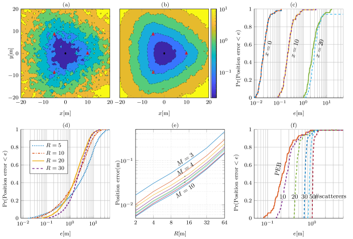
Figure 2: The position error (in meters) for a system with one Tx at the origin (marked by a black circle), $M=3$ Rxs (marked by red triangles) uniformly located on a circle with radius $R=10$ on the plane $z=1$, and a user located on $[x,y,-3]$: (a) PEB for one random RIS configurations; (b) the average of PEB over $100$ random RIS configurations; (c) the CDF of PEB (solid lines) and estimation error (dashed lines) for $100$ random RIS configurations at $[x,0,-3]$ $x\in\{0,10,20\}$; (d) the CDF of average PEB for $41\times 41$ equispaced user locations shown in subfigure (a) with $R\in\{5,10,20,30\}$; (e) average PEB at $[0,0,-3]$ for $M=3\dots 10$; (f) average PEB (solid line) and the estimation error (dashed lines) for $100$ random RIS configurations at $[10,0,-3]$ in the presence of $10,20,30,40,$ and $50$ scatterers.

Without loss of generality, we set $\bm{p}_{0}=\bm{0}$. In the absence of noise and based on (14), we have that $(\Delta_{n,m}-\|\bm{x}_{n}\|)^{2}=\|\bm{x}_{n}-\bm{p}_{m}\|^{2}$, which leads to

$$\bm{p}_{m}^{\top}\bm{x}-\Delta_{n,m}\|\bm{x}_{n}\| =\frac{1}{2}(\|\bm{p}_{m}\|^{2}-\Delta_{n,m}^{2}).$$ (19)

We can rewrite (19) in the matrix form as $\bm{P}\bm{x}_{n}=\bm{z}_{n}+\bm{\Delta}_{n}\|\bm{x}_{n}\|$, where $\bm{P}=[\bm{p}_{1},\bm{p}_{2},\dots,\bm{p}_{M}]^{\top}$, $\bm{z}=0.5[\|\bm{p}_{1}\|^{2}-\Delta_{n,1}^{2},\dots,\|\bm{p}_{M}\|^{2}-\Delta_{n,M}^{2}]^{\top}$. Then the $n$th user position can be estimated as [17]

$$\hat{\bm{x}}_{n} =\bm{a}_{n}+\bm{b}_{n}\|\hat{\bm{x}}_{n}\|$$ (20)

where $\bm{a}_{n}=(\bm{P}^{\top}\bm{P})^{-1}\bm{P}^{\top}\bm{z}_{n}$, $\bm{b}_{n}=(\bm{P}^{\top}\bm{P})^{-1}\bm{P}^{\top}\bm{\Delta}$, and

$$\|\hat{\bm{x}}_{n}\| =\frac{-\bm{a}_{n}^{\top}\bm{b}_{n}\pm\sqrt{(\bm{a}_{n}^{\top}\bm{b}_{n})^{2}-\|\bm{a}_{n}\|^{2}(\|\bm{b}_{n}\|^{2}-1)}}{\|\bm{b}_{n}\|^{2}-1}.$$ (21)

If (21) yields two viable solutions, one can insert both solutions to the negative log-likelihood function, which is the objective function in (18). If the outcome for one of the solutions is much smaller than the other one, then it should be used as the initial guess for the $n$th user position. However, if both outcomes are small, this indicates that the $M$ ellipsoids in (14) intersect in two distinct points. In such a case some prior knowledge (e.g., the user is located in a given region in relation to the Rxs) should be used to localize the user.

IV Simulation Results

In this section, we evaluate the estimation error of the user position and compare it to the theoretical PEB. The RIS is a $256\times 256$ uniform planar array (UPA). The clock biases $B_{m}$ are selected uniformly in the interval $[0,1/\Delta f)$. Since there is no interference between the LOS path and the NLOS paths from different users, the performance of the estimator for each user is independent of the number of users $N$ (as long as $T>N$) and therefore, we set $N=1$. For the LOS path, the channel gain $\alpha_{0,m}$ is calculated based on Friis’ formula assuming unit directivity for Tx and Rxs. For the NLOS path the channel gain is calculated as [18, Eq. (21)–(23)]

$$\gamma_{n,0}\gamma_{n,m}=\frac{\lambda^{2}(\cos(\theta_{n,m})\cos(\phi_{n,0}))^{0.285}}{16\pi\|\bm{p}_{0}-\bm{x}_{n}\|\|\bm{p}_{m}-\bm{x}_{n}\|}.$$ (22)

All the rotational angles corresponding to the user orientation is set to zero ($\bm{R}_{n}=\bm{I}_{3},\ \forall n$). The diagonal elements of $\bm{\Omega}_{n}$ are drawn randomly and independently from the unit circle. The presented results are obtained by averaging over $10,000$ random realization of RIS phase profiles ($100$) and noise ($100$ for each RIS phase profile). In our estimator, we use the prior knowledge that the UE is below the Rxs to resolve the sign ambiguity in (21). The rest of the system parameters are represented in Table I.

TABLE I: Parameters used in the simulation.

Parameter	Symbol	Value
Wavelength	$\lambda$	$1\ {\mathrm{cm}}$
RIS element spacing	$d$	$0.5\ {\mathrm{cm}}$
Light speed	$c$	$3\times 10^{8}\ \mathrm{m/s}$
Number of subcarriers	$K$	$100$
Subcarrier bandwidth	$\Delta f$	$120\ \mathrm{kHz}$
Number of transmissions	$T$	$32$
Transmission Power	$KE_{\mathrm{s}}\Delta f$	$25\ \mathrm{dBm}$
Noise PSD	$N_{0}$	$-174\ \mathrm{dBm/Hz}$
UE’s Noise figure	$n_{f}$	$5\ \mathrm{dB}$
FFT dimensions	$F$	$1024$

In Fig. 2 the position error has been analyzed for a system with the Tx at the origin, $M=3$ Rxs located on a circle with radius $R=3\ \mathrm{m}$ on the plane $z=1\ \mathrm{m}$, and a user located on $z=-3\ \mathrm{m}$. Fig. 2(a) illustrates the PEB for one realization of the RIS phase profile while Fig. 2(b) does so for the average of the PEB over $100$ random RIS configurations. It is evident that submeter localization accuracy can be attained in a large area around the Tx. From Fig. 2(b) one can see that the average PEB gradually and symmetrically increases with the distance from the Tx. In general, the same behavior can be observed also in Fig. 2(a), however, the increase in PEB is not smooth and symmetrical, which is due to different RIS reflection gains in different directions for a random phase profile. Fig. 2(c) represents the cumulative distribution function (CDF) of the PEB and the estimation error for $100$ RIS configurations at three points. It can be seen that the presented estimator tightly attains the the PEB as long as the PEB is less than $8$ meters.

In Fig. 2(d) we study the effect of Rx placement on the average PEB. To do so, we evaluate the CDF of the average PEB for a $41$ grid of UE locations over the area shown in Fig. 2(a). We consider four different values for the horizontal distance from Rx to Tx ($R$). It can be seen that for the majority of UE locations $R=20\ \mathrm{m}$ obtains superior position accuracy. This indicates that Rxs should be placed close to the edge of the region of interest to improve the (worst-case) localization accuracy.

In Fig. 2(e) the PEB at a UE position equal to $[0,0,-3]$ is calculated for different Rx numbers ($M$) and positions ($R$) of receivers. It can be seen that PEB increases with $R$ linearly, which is due to the quadratic decrease of SNR. Furthermore, it is evident that the improvement in PEB achieved by increasing the number of Rxs is noticeable only for low values of $M$.

Fig. 2(f) illustrates the PEB and the estimation error at the UE position $[10,0,-3]$ for $100$ realizations of RIS configuration in the presence of additional scatterers. The scatterers are placed randomly one meter below the UEs and within $10\,\mathrm{m}$ radius of the point $[0,0,-4]$. Since the scatterers are below the RIS, they only scatter the signal coming directly from the Tx onto them and not the reflected signals from the RISs. The channel gain for the scattered signal is calculated based on the radar range equation by assuming radar cross section of $0.1\,\mathrm{m}^{2}$. The interference from the scatterers deteriorates our estimation accuracy of the LOS delay $\hat{\tau}_{0,m}$, however, it does not affect that of the NLOS delay $\hat{\tau}_{n,m}$ ($n>0$). This is because the interference from scatterers cancels out upon calculating $\bm{r}_{n,m}=(1/T)\bm{Y}_{m}\bm{\omega}_{n}^{*}$ since we have $\bm{1}_{T}^{\top}\bm{\omega}_{n}^{*}=0,\forall n>0$. With a large number of scatterers, the position error is mainly affected by the error in LOS ToA estimation and therefore is predominantly independent of RIS phase profile, hence the sharp transition of CDF. Finally, we note that the estimator can perform properly even in the presence of a large number of scatterers and obtain submeter localization accuracy.

V Conclusion

We considered a multi-user RIS-enabled localization problem, where the users’ position in 3D was estimated by calculating the ToA of the LOS and NLOS paths at multiple receivers. The considered scenario can be categorized as a passive localization problem since the users do not generate transmitted signal or process received signals, but only reflect signals, based on which their positions are obtained. Nonetheless, it should be noted that RISs are not completely passive as they require some source of energy to reconfigure. We showed that by dividing the RIS phase profile to constant and time-varying parts and selecting the time-varying one based on orthogonal sequences, the interference between all the reflected NLOS signals among themselves and with the LOS paths can be avoided. In future work we aim to optimize the constant part of the RIS phase profile to improve the SNR of the NLOS path and achieve better localization accuracy. Extending the work to account for the limitations in RIS phase resolution and RIS synchronization is also an interesting future direction.

References

- [1] D. Dardari, “Communicating with large intelligent surfaces: Fundamental limits and models,” IEEE J. Select. Areas Commun., vol. 38, no. 11, pp. 2526–2537, Nov. 2020.
- [2] C. De Lima, et al., “Convergent communication, sensing and localization in 6G systems: An overview of technologies, opportunities and challenges,” IEEE Access, vol. 9, pp. 26 902–26 925, 2021.
- [3] H. Wymeersch, J. He, B. Denis, A. Clemente, and M. Juntti, “Radio localization and mapping with reconfigurable intelligent surfaces: Challenges, opportunities, and research directions,” IEEE Vehicular Technology Magazine, vol. 15, no. 4, pp. 52–61, Dec. 2020.
- [4] A. Shahmansoori, G. E. Garcia, G. Destino, G. Seco-Granados, and H. Wymeersch, “Position and orientation estimation through millimeter-wave MIMO in 5G systems,” IEEE Trans. Wireless Commun., vol. 17, no. 3, pp. 1822–1835, Mar. 2018.
- [5] J. Hong and T. Ohtsuki, “Signal eigenvector-based device-free passive localization using array sensor,” IEEE Trans. Vehicular Tech., vol. 64, no. 4, pp. 1354–1363, Apr. 2015.
- [6] L. M. Ni, D. Zhang, and M. R. Souryal, “RFID-based localization and tracking technologies,” IEEE Wireless Commun., vol. 18, no. 2, pp. 45–51, Apr. 2011.
- [7] H. Qin, Y. Peng, and W. Zhang, “Vehicles on RFID: Error-cognitive vehicle localization in GPS-less environments,” IEEE Trans. Vehicular Tech., vol. 66, no. 11, pp. 9943–9957, Nov. 2017.
- [8] W. Ruan, L. Yao, Q. Z. Sheng, N. J. Falkner, and X. Li, “Tagtrack: Device-free localization and tracking using passive RFID tags,” in Proceedings of the 11th Int. Conf. on Mobile and Ubiquitous System, London, UK, Dec. 2014, pp. 80–89.
- [9] J. Shen, A. F. Molisch, and J. Salmi, “Accurate passive location estimation using TOA measurements,” IEEE Trans. Wireless Commun., vol. 11, no. 6, pp. 2182–2192, Jun. 2012.
- [10] Y. Wang, S. Ma, and C. P. Chen, “TOA-based passive localization in quasi-synchronous networks,” IEEE Commun. Lett., vol. 18, no. 4, pp. 592–595, Feb. 2014.
- [11] W. Yuan, N. Wu, B. Etzlinger, Y. Li, C. Yan, and L. Hanzo, “Expectation–maximization-based passive localization relying on asynchronous receivers: Centralized versus distributed implementations,” IEEE Trans. Commun., vol. 67, no. 1, pp. 668–681, Jan. 2019.
- [12] N. Decarli, F. Guidi, and D. Dardari, “A novel joint RFID and radar sensor network for passive localization: Design and performance bounds,” IEEE J. Select. Areas Commun., vol. 8, no. 1, pp. 80–95, Feb. 2014.
- [13] X. Zhang, H. Li, J. Liu, and B. Himed, “Joint delay and Doppler estimation for passive sensing with direct-path interference,” IEEE Transactions on Signal Processing, vol. 64, no. 3, pp. 630–640, 2016.
- [14] K. Keykhosravi, M. F. Keskin, G. Seco-Granados, and H. Wymeersch, “SISO RIS-enabled joint 3D downlink localization and synchronization,” accepted in IEEE Int. Conf. Commun. (ICC), Montreal, Canada, Jun. 2021, available in arXiv preprint:2011.02391.
- [15] P. Fan, “Spreading sequence design and theoretical limits for quasisynchronous CDMA systems,” EURASIP J. on wireless Commun. and Net., vol. 2004, no. 1, pp. 1–13, Mar. 2004.
- [16] S. M. Kay, Fundamentals of statistical signal processing: Estimation Theory. Prentice Hall PTR, 1993.
- [17] M. Malanowski, “An algorithm for 3D target localization from passive radar measurements,” in Photon. Appl. in Astron., Commun., Industry, and High-Energy Phys. Exp., Wilga, Poland, May 2009.
- [18] S. W. Ellingson, “Path loss in reconfigurable intelligent surface-enabled channels,” arXiv preprint arXiv:1912.06759, 2019.