Improved Analysis and Rates for Variance Reduction under Without-replacement Sampling Orders

Abstract

When applying a stochastic algorithm, one must choose an order to draw samples. The practical choices are without-replacement sampling orders, which are empirically faster and more cache-friendly than uniform-iid-sampling but often have inferior theoretical guarantees. Without-replacement sampling is well understood only for SGD without variance reduction. In this paper, we will improve the convergence analysis and rates of variance reduction under without-replacement sampling orders for composite finite-sum minimization.

Our results are in two-folds. First, we develop a damped variant of Finito called Prox-DFinito and establish its convergence rates with random reshuffling, cyclic sampling, and shuffling-once, under both convex and strongly convex scenarios. These rates match full-batch gradient descent and are state-of-the-art compared to the existing results for without-replacement sampling with variance-reduction. Second, our analysis can gauge how the cyclic order will influence the rate of cyclic sampling and, thus, allows us to derive the optimal fixed ordering. In the highly data-heterogeneous scenario, Prox-DFinito with optimal cyclic sampling can attain a sample-size-independent convergence rate, which, to our knowledge, is the first result that can match with uniform-iid-sampling with variance reduction. We also propose a practical method to discover the optimal cyclic ordering numerically.

1 Introduction

We study the finite-sum composite optimization problem

$$\min_{x\in\mathbb{R}^{d}}\ F(x)+r(x)\quad\mbox{and}\quad F(x)=\frac{1}{n}\sum_{i=1}^{n}f_{i}(x).$$ (1)

where each $f_{i}(x)$ is differentiable and convex, and the regularization function $r(x)$ is convex but not necessarily differentiable. This formulation arises in many problems in machine learning [34, 39, 14], distributed optimization [20, 3, 19], and signal processing [4, 9].

Table 1: Number of individual gradient evaluations needed by each algorithm to reach an $\epsilon$-accurate solution. Notation $\tilde{{\mathcal{O}}}(\cdot)$ hides logarithmic factors. Error metrics $(\mathbb{E})\|\nabla F(x)\|^{2}$ and $(\mathbb{E})\|x-x^{\star}\|^{2}$ are used for convex and strongly convex problems, respectively.

Algorithm	Supp. Prox	Sampling	Asmp⋄	Convex	Strongly Convex
Prox-GD	Yes	Full-batch	$F(x)$	${\mathcal{O}}(n\frac{L^{2}}{\epsilon})$	${\mathcal{O}}(n\frac{L}{\mu}\log(\frac{1}{\epsilon}))$
SGD [22]	No	Cyclic	$f_{i}(x)$	${\mathcal{O}}(n(\frac{L}{\epsilon})^{\frac{3}{2}})$	${\mathcal{O}}(n(\frac{L}{\mu})^{\frac{3}{2}}\frac{1}{\sqrt{\epsilon}})$
SGD [22]	No	RR	$f_{i}(x)$	${\mathcal{O}}(n^{\frac{1}{2}}(\frac{L}{\epsilon})^{\frac{3}{2}})$	${\mathcal{O}}({\sqrt{n}}(\frac{L}{\mu})^{\frac{3}{2}}\frac{1}{\sqrt{\epsilon}})$
PSGD [21]	Yes	RR	$f_{i}(x)$	$\diagdown$	${\mathcal{O}}(n(\frac{L}{\mu})^{\frac{3}{2}}\frac{1}{\sqrt{\epsilon}})$
PIAG [35]	Yes	Cyclic/RR	$F(x)$	$\diagdown$	${\mathcal{O}}(n\frac{L}{\mu}\log(\frac{1}{\epsilon}))$
AVRG [37]	No	RR	$f_{i}(x)$	$\diagdown$	${\mathcal{O}}(n(\frac{L}{\mu})^{2}\log(\frac{1}{\epsilon}))$
SAGA  [33]	Yes	Cyclic	$f_{i}(x)$	${\mathcal{O}}(n^{3}\frac{L^{2}}{\epsilon})$	${\mathcal{O}}(n^{3}(\frac{L}{\mu})^{2}\log(\frac{1}{\epsilon}))$
SVRG  [33]	Yes	Cyclic	$f_{i}(x)$	${\mathcal{O}}(n^{3}\frac{L^{2}}{\epsilon})$	${\mathcal{O}}(n^{3}(\frac{L}{\mu})^{2}\log(\frac{1}{\epsilon}))$
DIAG [23]	No	Cyclic	$f_{i}(x)$	$\diagdown$	${\mathcal{O}}(n\frac{L}{\mu}\log(\frac{1}{\epsilon}))$
Cyc. Cord. Upd  [5]	Yes	Cyclic/RR	$f_{i}(x)$	${\mathcal{O}}(n2^{n}\frac{L^{2}}{\epsilon})$	${\mathcal{O}}(n(\frac{L}{\mu})^{3}\log(\frac{1}{\epsilon}))$
SVRG [18]♣	No	Cyclic/RR	$F(x)$	${\mathcal{O}}(n\frac{L^{2}}{\epsilon})$	${\mathcal{O}}(n(\frac{L}{\mu})^{\frac{3}{2}}\log(\frac{1}{\epsilon}))$
SVRG [18]♣	No	RR	$F(x)$	${\mathcal{O}}(n\frac{L^{2}}{\epsilon})$	${\mathcal{O}}(n\frac{L}{\mu}\log(\frac{1}{\epsilon}))^{\dagger}$
SVRG [18]♣	No	RR	$f_{i}(x)$	${\mathcal{O}}(n\frac{L^{2}}{\epsilon})$	${\mathcal{O}}(n^{\frac{1}{2}}(\frac{L}{\mu})^{\frac{3}{2}}\log(\frac{1}{\epsilon}))^{\dagger}$
Prox-DFinito (Ours)	Yes	RR	$f_{i}(x)$	${{\mathcal{O}}}(n\frac{L^{2}}{\epsilon})$	${\mathcal{O}}(n\frac{L}{\mu}\log(\frac{1}{\epsilon}))$
Prox-DFinito (Ours)	Yes	worst cyc. order	$f_{i}(x)$	$\tilde{{\mathcal{O}}}(n\frac{L^{2}}{\epsilon})$	$\tilde{{\mathcal{O}}}(n\frac{L}{\mu}\log(\frac{1}{\epsilon}))$
Prox-DFinito (Ours)	Yes	best cyc. order	$f_{i}(x)$	$\tilde{{\mathcal{O}}}(\frac{L^{2}}{\epsilon})^{\ddagger}$	$\tilde{{\mathcal{O}}}(n\frac{L}{\mu}\log(\frac{1}{n\epsilon}))^{\ddagger}$
⋄ The “Assumption” column indicates the scope of smoothness and strong convexity, where $F(x)$ means
smoothness and strong convexity in the average sense and $f_{i}(x)$ assumes smoothness and strong convexity
for each summand function.
♣[18] is an independent and concurrent work.
† This complexity is attained under big data regime: $n>{\mathcal{O}}(\frac{L}{\mu})$.
‡ This complexity can be attained in a highly heterogeneous scenario, see details in Sec 4.2.

The leading methods to solve (1) are first-order algorithms such as stochastic gradient descent (SGD) [28, 2] and stochastic variance-reduced methods [14, 6, 7, 17, 10, 32]. In the implementation of these methods, each $f_{i}(x)$ can be sampled either with or without replacement. Without-replacement sampling draws each $f_{i}(x)$ exactly once during an epoch, which is numerically faster than with-replacement sampling and more cache-friendly; see the experiments in [1, 38, 11, 7, 37, 5]. This has triggered significant interests in understanding the theory behind without-replacement sampling.

Among the most popular without-replacement approaches are cyclic sampling, random reshuffling, and shuffling-once. Cyclic sampling draws the samples in a cyclic order. Random reshuffling reorders the samples at the beginning of each sample epoch. The third approach, however, shuffles data only once before the training begins. Without-replacement sampling have been extensively studied for SGD. It was established in [1, 38, 11, 22, 24] that without-replacement sampling enables SGD with faster convergence For example, it was proved that without-replacement sampling can speed up uniform-iid-sampling SGD from $\tilde{{\mathcal{O}}}(1/k)$ to $\tilde{{\mathcal{O}}}(1/k^{2})$ (where $k$ is the iteration) for strongly-convex costs in [11, 12], and ${\mathcal{O}}(1/k^{1/2})$ to ${\mathcal{O}}(1/k)$ for the convex costs in [24, 22]. [31] establishes a tight lower bound for random reshuffling SGD. Recent works [27, 22] close the gap between upper and lower bounds. Authors of [22] also analyzes without-replacement SGD with non-convex costs.

In contrast to the mature results in SGD, variance-reduction under without-replacement sampling are less understood. Variance reduction strategies construct stochastic gradient estimators with vanishing gradient variance, which allows for much larger learning rate and hence speed up training process. Variance reduction under without-replacement sampling is difficult to analyze. In the strongly convex scenario, [37, 33] provide linear convergence guarantees for SVRG/SAGA with random reshuffling, but the rates are worse than full-batch gradient descent (GD). Authors of [35, 23] improved the rate so that it can match with GD. In convex scenario, existing rates for without-replacement sampling with variance reduction, except for the rate established in an independent and concurrent work [18], are still far worse than GD [33, 5], see Table 1. Furthermore, no existing rates for variance reduction under without-replacement sampling orders, in either convex or strongly convex scenarios, can match those under uniform-iid-sampling which are essentially sample-size independent. There is a clear gap between the known convergence rates and superior practical performance for without-replacement sampling with variance reduction.

1.1 Main results

This paper narrows such gap by providing convergence analysis and rates for proximal DFinito, a proximal damped variant of Finito/MISO [7, 17, 26], which is a well-known variance reduction algorithm, under without-replacement sampling orders. Our main achieved results are:

• We develop a proximal damped variant of Finito/MISO called Prox-DFinito and establish its gradient complexities with random reshuffling, cyclic sampling, and shuffling-once, under both convex and strongly convex scenarios. All these rates match with gradient descent, and are state-of-the-art (up to logarithm factors) compared to existing results for without-replacement sampling with variance-reduction, see Table 1.

• Our novel analysis can gauge how a cyclic order will influence the rate of Prox-DFinito with cyclic sampling. This allows us to identify the optimal cyclic sampling ordering. Prox-DFinito with optimal cyclic sampling, in the highly data-heterogeneous scenario, can attain a sample-size-independent convergence rate, which is the first result, to our knowledge, that can match with uniform-iid-sampling with variance reduction in certain scenarios. We also propose a numerical method to discover the optimal cyclic ordering cheaply.

1.2 Other related works

Our analysis on cyclic sampling is novel. Most existing analyses unify random reshuffling and cyclic sampling into the same framework; see the SGD analysis in [11], the variance-reduction analysis in [10, 36, 23, 37], and the coordinate-update analysis in [5]. These analyses are primarily based on the “sampled-once-per-epoch” property and do not analyze the orders within each epoch, so they do not distinguish cyclic sampling from random reshuffling in analysis. [16] finds that random reshuffling SGD is basically the average over all cyclic sampling trials. This implies cyclic sampling can outperform random reshuffling with a well-designed sampling order. However, [16] does not discuss how much better cyclic sampling can outperform random reshuffling and how to achieve such cyclic order. Different from existing literatures, our analysis introduces an order-specific norm to gauge how cyclic sampling performs with different fixed orders. With such norm, we are able to clarify the worst-case and best-case performance of variance reduction with cyclic sampling.

Simultaneously and independently, a recent work [18] also provided an improved rates for variance reduction under without-replacement sampling orders that can match with gradient descent. However, [18] does not discuss whether and when variance reduction with replacement sampling can match with uniform sampling. In addition, [18] studies SVRG while this paper studies Finito/MISO. The convergence analyses in these two works are very different. The detailed comparison between this work and [18] can be referred to Sec. 3.3.

1.3 Notations

Throughout the paper we let $\mathrm{col}\{x_{1},\cdots,x_{n}\}$ denote a column vector formed by stacking $x_{1},\cdots,x_{n}$. We let $[n]:=\{1,\cdots,n\}$ and define the proximal operator as

$${\mathbf{prox}}_{\alpha r}(x):=\arg\min_{y\in\mathbb{R}^{d}}\{\alpha\,r(y)+\frac{1}{2}\|y-x\|^{2}\}$$ (2)

which is single-valued when $r$ is convex, closed and proper. In general, we say ${\mathcal{A}}$ is an operator and write ${\mathcal{A}}:{\mathcal{X}}\rightarrow{\mathcal{Y}}$ if ${\mathcal{A}}$ maps each point in space ${\mathcal{X}}$ to another space ${\mathcal{Y}}$. So ${\mathcal{A}}({\boldsymbol{x}})\in{\mathcal{Y}}$ for all ${\boldsymbol{x}}\in{\mathcal{X}}$. For simplicity, we write ${\mathcal{A}}{\boldsymbol{x}}={\mathcal{A}}({\boldsymbol{x}})$ and ${\mathcal{A}}\circ{\mathcal{B}}{\boldsymbol{x}}={\mathcal{A}}({\mathcal{B}}({\boldsymbol{x}}))$ for operator composition.

Cyclic sampling. We define $\pi:=(\pi(1),\pi(2),\dots,\pi(n))$ as an arbitrary determined permutation of sample indexes. The order $\pi$ is fixed throughout the entire learning process under cyclic sampling.

Random reshuffling. When starting each epoch, a random permutation $\tau:=(\tau(1),\tau(2),...,\tau(n))$ is generated to specify the order to take samples. Let $\tau_{k}$ denote the permutation of the $k$-th epoch.

2 Proximal Finito/MISO with Damping

The proximal gradient method to solve problem (1) is

$$z_{i}^{t} =x^{t-1}-\alpha\nabla f_{i}(x^{t-1}),\quad\forall\ i\in[n]$$ (3a)

$$x^{t} ={\mathbf{prox}}_{\alpha r}\big{(}\frac{1}{n}\sum_{i=1}^{n}z_{i}^{t}\big{)}$$ (3b)

Algorithm 1 Prox-DFinito

  Input: $\bar{z}^{0}=\frac{1}{n}\sum\limits_{i=1}^{n}z_{i}^{0}$, step-size $\alpha$, and $\theta\in(0,1)$;

  for epoch $k=0,1,2,\cdots$ do

     for iteration $t=kn+1,kn+2,\cdots,(k+1)n$ do

        $x^{t-1}={\mathbf{prox}}_{\alpha r}(\bar{z}^{t-1})$;

        Pick $i_{t}$ with some rule;

        Update $z_{i_{t}}^{t}$ and $\bar{z}^{t}$ according to (4c) and (5);

     end for

     $z_{i}^{(k+1)n}\leftarrow(1-\theta)z_{i}^{kn}+\theta z_{i}^{(k+1)n}$ for any $i\in[n]$; $\quad\triangleright$ a damping step

     $\bar{z}^{(k+1)n}\leftarrow(1-\theta)\bar{z}^{kn}+\theta\bar{z}^{(k+1)n}$; $\hskip 71.13188pt\triangleright$ a damping step

  end for

To avoid the global average that passes over all samples, we propose to update one $z_{i}$ per iteration:

$$z_{i}^{t} =\left\{\begin{array}[]{ll}x^{t-1}-\alpha\nabla f_{i}(x^{t-1}),&\quad i=i_{t}\\ z_{i}^{t-1},&\quad i\neq i_{t}\end{array}\right.$$ (4c)

$$x^{t} ={\mathbf{prox}}_{\alpha r}\big{(}\frac{1}{n}\sum_{i=1}^{n}z_{i}^{t}\big{)}.$$ (4d)

When $i_{t}$ is invoked with uniform-iid-sampling and $r(x)=0$, algorithm (4c)–(4d) reduces to Finito/MISO [7, 17]. When $i_{t}$ is invoked with cyclic sampling and $r(x)=0$, algorithm (4c)–(4d) reduces to DIAG [23] and WPG [19]. We let $\bar{z}^{t}:=\frac{1}{n}\sum_{i=1}^{n}z_{i}^{t}$. The update (4c) yields

$$\bar{z}^{t}=\bar{z}^{t-1}+(z^{t}_{i_{t}}-z^{t-1}_{i_{t}})/n.$$ (5)

This update can be finished with ${\mathcal{O}}(d)$ operations if $\{z^{t}_{i}\}_{i=1}^{n}$ are stored with ${\mathcal{O}}(nd)$ memory. Furthermore, to increase robustness and simplify the convergence analysis, we impose a damping step to $z_{i}$ and $\bar{z}$ when each epoch finishes. The proximal damped Finito/MISO method is listed in Algorithm 1. Note that the damping step does not incur additional memory requirements. A more practical implementation of Algorithm 1 is referred to Algorithm 3 in Appendix A.

2.1 Fixed-point recursion reformulation

Algorithm (4c)–(4d) can be reformulated into a fixed-point recursion in $\{z_{i}\}_{i=1}^{n}$. Such a fixed-point recursion will be utilized throughout the paper. To proceed, we define ${\boldsymbol{z}}=\mathrm{col}\{z_{1},\cdots,z_{n}\}\in\mathbb{R}^{nd}$ and introduce the average operator ${\mathcal{A}}:\mathbb{R}^{nd}\rightarrow\mathbb{R}^{d}$ as ${\mathcal{A}}{\boldsymbol{z}}=\frac{1}{n}\sum_{i=1}^{n}z_{i}$. We further define the $i$-th block coordinate operator ${\mathcal{T}}_{i}:\mathbb{R}^{nd}\to\mathbb{R}^{nd}$ as

$${\mathcal{T}}_{i}{\boldsymbol{z}}=\mathrm{col}\{z_{1},\cdots,(I-\alpha\nabla f_{i})\circ{\mathbf{prox}}_{\alpha r}({\mathcal{A}}{\boldsymbol{z}}),\cdots,z_{n}\}$$

where $I$ denotes the identity mapping. When applying ${\mathcal{T}}_{i}$, it is noted that the $i$-th block coordinate in ${\boldsymbol{z}}$ is updated while the others remain unchanged.

Proposition 1.

Prox-DFinito with fixed cyclic sampling order $\pi$ is equivalent to the following fixed-point recursion (see proof in Appendix B.1.)

$${\boldsymbol{z}}^{(k+1)n}=(1-\theta){\boldsymbol{z}}^{kn}+\theta{\mathcal{T}}_{\pi}{\boldsymbol{z}}^{kn}$$ (6)

where ${\mathcal{T}}_{\pi}={\mathcal{T}}_{\pi(n)}\circ\cdots\circ{\mathcal{T}}_{\pi(1)}$. Furthermore, variable $x^{t}$ can be recovered by

$$x^{t}={\mathbf{prox}}_{\alpha r}\circ{\mathcal{A}}{\boldsymbol{z}}^{t},\quad t=0,1,2,\cdots$$ (7)

Similar result also hold for random reshuffling scenario.

Proposition 2.

Prox-DFinito with random reshuffling is equivalent to

$${\boldsymbol{z}}^{(k+1)n}=(1-\theta){\boldsymbol{z}}^{kn}+\theta{\mathcal{T}}_{\tau_{k}}{\boldsymbol{z}}^{kn}$$ (8)

where ${\mathcal{T}}_{\tau_{k}}={\mathcal{T}}_{\tau_{k}(n)}\circ\cdots\circ{\mathcal{T}}_{\tau_{k}(1)}$. Furthermore, variable $x^{t}$ can be recovered by following (7).

2.2 Optimality condition

Assume there exists $x^{\star}$ that minimizes $F(x)+r(x)$, i.e., $0\in\nabla F(x^{\star})+\partial\,r(x^{\star})$. Then the relation between the minimizer $x^{\star}$ and the fixed-point ${\boldsymbol{z}}^{\star}$ of recursion (6) and (8) can be characterized as:

Proposition 3.

$x^{\star}$ minimizes $F(x)+r(x)$ if and only if there is ${\boldsymbol{z}}^{\star}$ so that (proof in Appendix B.2)

$${\boldsymbol{z}}^{\star} ={\mathcal{T}}_{i}{\boldsymbol{z}}^{\star},\quad\forall\,i\in[n],$$ (9)

$$x^{\star} ={\mathbf{prox}}_{\alpha r}\circ{\mathcal{A}}{\boldsymbol{z}}^{\star}.$$ (10)

Remark 1.

If $x^{\star}$ minimizes $F(x)+r(x)$, it holds from (9) and (10) that $z_{i}^{\star}=(I-\alpha\nabla f_{i})\circ{\mathbf{prox}}_{\alpha r}({\mathcal{A}}{\boldsymbol{z}}^{\star})=x^{\star}-\alpha\nabla f_{i}(x^{\star})$ for any $i\in[n]$.

2.3 An order-specific norm

To gauge the influence of different sampling orders, we now introduce an order-specific norm.

Definition 1.

Given ${\boldsymbol{z}}=\mbox{col}\{z_{1},\cdots,z_{n}\}\in\mathbb{R}^{nd}$ and a fixed cyclic order $\pi$, we define

$$\|{\boldsymbol{z}}\|^{2}_{\pi} =\sum_{i=1}^{n}\frac{i}{n}\|z_{\pi(i)}\|^{2}=\frac{1}{n}\|z_{\pi(1)}\|^{2}+\frac{2}{n}\|z_{\pi(2)}\|^{2}+\cdots+\|z_{\pi(n)}\|^{2}$$

as the $\pi$-specific norm.

For two different cyclic orders $\pi$ and $\pi^{\prime}$, it generally holds that $\|{\boldsymbol{z}}\|^{2}_{\pi}\neq\|{\boldsymbol{z}}\|^{2}_{\pi^{\prime}}$. Note that the coefficients in $\|{\boldsymbol{z}}\|^{2}_{\pi}$ are delicately designed for technical reasons (see Lemma 1 and its proof in the appendix). The order-specific norm facilitates the performance comparison between two orderings.

3 Convergence Analysis

In this section we establish the convergence rate of Prox-DFinito with cyclic sampling and random reshuffling in convex and strongly convex scenarios, respectively.

3.1 The convex scenario

We first study the convex scenario under the following assumption:

Assumption 1 (Convex).

Each function $f_{i}(x)$ is convex and $L$-smooth.

It is worth noting that the convergence results on cyclic sampling and random reshuffling for the convex scenario are quite limited except for [22, 33, 5, 18].

Cyclic sampling and shuffling-once. We first introduce the following lemma showing that ${\mathcal{T}}_{\pi}$ is non-expansive with respect to $\|\cdot\|_{\pi}$, which is fundamental to the convergence analysis.

Lemma 1.

Under Assumption 1, if step-size $0<\alpha\leq\frac{2}{L}$ and the data is sampled with a fixed cyclic order $\pi$, it holds that (see proof in Appendix C.1)

$$\|{\mathcal{T}}_{\pi}{\boldsymbol{u}}-{\mathcal{T}}_{\pi}{\boldsymbol{v}}\|_{\pi}^{2}\leq\|{\boldsymbol{u}}-{\boldsymbol{v}}\|_{\pi}^{2},\quad\forall\,{\boldsymbol{u}},{\boldsymbol{v}}\in\mathbb{R}^{nd}.$$ (11)

Recall (6) that the sequence ${\boldsymbol{z}}^{kn}$ is generated through ${\boldsymbol{z}}^{(k+1)n}={\mathcal{S}}_{\pi}{\boldsymbol{z}}^{(kn)}$. Since ${\mathcal{S}}_{\pi}=(1-\theta)I+\theta{\mathcal{T}}_{\pi}$ and ${\mathcal{T}}_{\pi}$ is non-expansive, we can prove the distance $\|{\boldsymbol{z}}^{(k+1)n}-{\boldsymbol{z}}^{(kn)}\|^{2}$ will converge to $0$ sublinearly:

Lemma 2.

Under Assumption 1, if step-size $0<\alpha\leq\frac{2}{L}$ and the data is sampled with a fixed cyclic order $\pi$, it holds for any $k=0,1,\cdots$ that (see proof in Appendix

$$\|{\boldsymbol{z}}^{(k+1)n}-{\boldsymbol{z}}^{kn}\|^{2}_{\pi}\leq\frac{\theta}{(k+1)(1-\theta)}\|{\boldsymbol{z}}^{0}-{\boldsymbol{z}}^{\star}\|^{2}_{\pi}$$ (12)

where $\theta\in(0,1)$ is the damping parameter.

With Lemma 2 and the relation between $x^{t}$ and ${\boldsymbol{z}}^{t}$ in (7), we can establish the convergence rate:

Theorem 1.

Under Assumption 1, if step-size $0<\alpha\leq\frac{2}{L}$ and the data is sampled with a fixed cyclic order $\pi$, it holds that (see proof in Appendix C.3)

$$\min\limits_{g\in\partial\,r(x^{kn})}\|\nabla F(x^{kn})+g\|^{2}\leq\frac{CL^{2}}{(k+1)\theta(1-\theta)}$$ (13)

where $\theta\in(0,1)$ and $C=\left(\frac{2}{\alpha L}\right)^{2}\frac{\log(n)+1}{n}\|{\boldsymbol{z}}^{0}-{\boldsymbol{z}}^{\star}\|^{2}_{\pi}$.

Remark 2.

Inspired by reference [16], one can take expectation over cyclic order $\pi$ in (13) to obtain the convergence rate of Prox-DFinito shuffled once before training begins (with $C=\left(\frac{2}{\alpha L}\right)^{2}\frac{(n+1)(\log(n)+1)}{2n^{2}}\|{\boldsymbol{z}}^{0}-{\boldsymbol{z}}^{\star}\|^{2}$):

$$\mathbb{E}\,\min\limits_{g\in\partial\,r(x^{kn})}\|\nabla F(x^{kn})+g\|^{2}\leq\frac{CL^{2}}{(k+1)\theta(1-\theta)}$$ (14)

Random reshuffling. We let $\tau_{k}$ denote the sampling order used in the $k$-th epoch. Apparently, $\tau_{k}$ is a uniformly distributed random variable with $n!$ realizations. With the similar analysis technique, we can also establish the convergence rate under random reshuffling in the expectation sense.

Theorem 2.

Under Assumption 1, if step-size $0<\alpha\leq\frac{2}{L}$ and data is sampled with random reshuffling, it holds that (see proof in Appendix D.2)

$$\mathbb{E}\,\min\limits_{g\in\partial\,r(x^{kn})}\|\nabla F(x^{kn})+g\|^{2}\leq\frac{CL^{2}}{(k+1)\theta(1-\theta)}$$ (15)

where $\theta\in(0,1)$ and $C=\left(\frac{5}{3\alpha L}\right)^{2}\frac{1}{n}\|{\boldsymbol{z}}^{0}-{\boldsymbol{z}}^{\star}\|^{2}$.

Comparing (15) with (13), it is observed that random reshuffling replaces the constant $\|{\boldsymbol{z}}^{0}-{\boldsymbol{z}}^{\star}\|_{\pi}^{2}$ by $\|{\boldsymbol{z}}^{0}-{\boldsymbol{z}}^{\star}\|^{2}$ and removes the $\log(n)$ term in the upper bound.

3.2 The strongly convex scenario

In this subsection, we study the convergence rate of Prox-DFinito under the following assumption:

Assumption 2 (Strongly Convex).

Each function $f_{i}(x)$ is $\mu$-strongly convex and $L$-smooth.

Theorem 3.

Under Assumption 2, if step-size $0<\alpha\leq\frac{2}{\mu+L}$, it holds that (see proof in Appendix E)

$$(\mathbb{E})\,\|x^{kn}-x^{\star}\|^{2}\leq\big{(}1-\frac{2\theta\alpha\mu L}{\mu+L}\big{)}^{k}C$$ (16)

where $\theta\in(0,1)$ and

$$C=\begin{cases}\frac{\log(n)+1}{n}\|{\boldsymbol{z}}^{0}-{\boldsymbol{z}}^{\star}\|_{\pi}^{2}\,\,\mbox{with $\pi$-order cyclic sampling},\\ \frac{1}{n}\|{\boldsymbol{z}}^{0}-{\boldsymbol{z}}^{\star}\|^{2}\,\,\mbox{with random reshuffling}.\end{cases}$$

Remark 3.

Note when $\theta\to 1$, Prox-DFinito actually reaches the best performance, so damping is essentially not necessary in strongly convex scenario.

3.3 Comparison with the existing results

Recalling $\|{\boldsymbol{z}}\|^{2}_{\pi}=\sum_{i=1}^{n}\frac{i}{n}\|z_{\pi(i)}\|^{2}$, it holds that

$$\frac{1}{n}\|{\boldsymbol{z}}\|^{2}\leq\|{\boldsymbol{z}}\|^{2}_{\pi}\leq\|{\boldsymbol{z}}\|^{2},\quad\forall{\boldsymbol{z}},\pi.$$ (17)

For a fair comparison with existing works, we consider the worst case performance of cyclic sampling by relaxing $\|{\boldsymbol{z}}^{0}-{\boldsymbol{z}}^{\star}\|^{2}_{\pi}$ to its upper bound $\|{\boldsymbol{z}}^{0}-{\boldsymbol{z}}^{\star}\|^{2}$. Letting $\alpha={\mathcal{O}}(1/L)$, $\theta=1/2$ and assuming $\frac{1}{n}\|{\boldsymbol{z}}^{0}-{\boldsymbol{z}}^{\star}\|^{2}={\mathcal{O}}(1)$, the convergence rates derived in Theorems 1–3 reduce to

C-Cyclic $$=\tilde{{\mathcal{O}}}\big{(}{L^{2}}/{k}\big{)},\hskip 39.83368pt\mbox{C-RR}={{\mathcal{O}}}\big{(}{L^{2}}/{k}\big{)}$$

SC-Cyclic $$=\tilde{{\mathcal{O}}}\big{(}(1-1/\kappa)^{k}\big{)},\hskip 14.22636pt\ \mbox{SC-RR}={{\mathcal{O}}}\big{(}(1-1/\kappa)^{k}\big{)}.$$

where “C” denotes “convex” and “SC” denotes “strongly convex”, $\kappa=L/\mu$, and $\tilde{{\mathcal{O}}}(\cdot)$ hides the $\log(n)$ factor. Note that all rates are in the epoch-wise sense. These rates can be translated into the the gradient complexity (equivalent to sample complexity) of Prox-DFinito to reach an $\epsilon$-accurate solution. The comparison with existing works are listed in Table 1.

Different metrics. Except for [5] and our Prox-DFinito algorithm whose convergence analyses are based on the gradient norm in the convex and smooth scenario, results in other references are based on function value metric (i.e., objective error $F(x^{kn})-F(x^{\star})$). The function value metric can imply the gradient norm metric, but not always vice versa. To comapre Prox-DFinito with other established results in the same metric, we have to transform the rates in other references into the gradient norm metric. The comparison is listed in Table 1. When the gradient norm metric is used, we observe that the rates of Prox-DFinito match that with gradient descent, and are state-of-the-art compared to the existing results. However, the rate of Prox-DFinito in terms of the function value is not known yet (this unknown rate may end up being worse than those of the other methods).

For the non-smooth scenario, our metric $\min_{g\in\partial r(x)}\|\nabla F(x)+\partial r(x)\|^{2}$ may not be bounded by the functional suboptimality $F(x)+r(x)-F(x^{\star})-r(x^{\star})$, and hence Prox-DFinito results are not comparable with those in [21, 35, 37, 33, 18]. The results listed in Table 1 are all for the smooth scenario of [21, 35, 37, 33, 18], and we use “Support Prox” to indicate whether the results cover the non-smooth scenario or not.

Assumption scope. Except for references [18, 35] and Proximal GD algorithm whose convergence analyses are conducted by assuming the average of each function to be $\bar{L}$-smooth (and perhaps $\bar{\mu}$-strongly convex), results in other references are based on a stronger assumption that each summand function to be $L$-smooth (and perhaps $\mu$-strongly convex). Note that $\bar{L}$ can be much smaller than $L$ sometimes. To compare [18, 35] and Proximal GD with other references under the same assumption, we let each ${L}=\bar{L}$ in Table 1. However, it is worth noting that when each $L_{i}$ is drastically different from each other and can be evaluated precisely, the results relying on $\bar{L}$ (e.g., [35] and [18]) can be much better than the results established in this work.

Comparison with GD. It is observed from Table 1 that Prox-DFinito with cyclic sampling or random reshuffling is no-worse than Proximal GD. It is the first no-worse-than-GD result, besides the independent and concurrent work [18], that covers both the non-smooth and the convex scenarios for variance-reduction methods under without-replacement sampling orders. The pioneering work DIAG [23] established a similar result only for smooth and strongly-convex problems.

Comparison with RR/CS methods. Prox-DFinito achieves the nearly state-of-the-art gradient complexity in both convex and strongly convex scenarios (except for the convex and smooth case due to the weaker metric adopted) among known without-replacement stochastic approaches to solving the finite-sum optimization problem (1), see Table 1. In addition, it is worth noting that in Table 1, algorithms of [33, 35, 23] and our Prox-DFinito have an ${\mathcal{O}}(nd)$ memory requirement while others only need ${\mathcal{O}}(d)$ memory. In other words, Prox-DFinito is memory-costly in spite of its superior theoretical convergence rate and sample complexity.

Comparison with uniform-iid-sampling methods. It is known that uniform-sampling variance-reduction can achieve an ${\mathcal{O}}(\max\{n,{L}/{\mu}\}\log({1}/{\epsilon}))$ sample complexity for strongly convex problems [14, 26, 6] and ${\mathcal{O}}({L^{2}}/{\epsilon})$ (when using metric $\mathbb{E}\|\nabla F(x)\|^{2}$) for convex problems [26]. In other words, these uniform-sampling methods have sample complexities that are independent of sample size $n$. Our achieved results (and other existing results listed in Table 1 and [18]) for random reshuffling or worst-case cyclic sampling cannot match with uniform-sampling yet. However, this paper establishes that Prox-DFinito with the optimal cyclic order, in the highly data-heterogeneous scenario, can achieve an $\tilde{{\mathcal{O}}}({L^{2}}/{\epsilon})$ sample complexity in the convex scenario, which matches with uniform-sampling up to a $\log(n)$ factor, see the detailed discussion in Sec. 4. To our best knowledge, it is the first result, at least in certain scenarios, that variance reduction under without-replacement sampling orders can match with its uniform-sampling counterpart in terms of their sample complexity upper bound. Nevertheless, it still remains unclear how to close the gap in sample complexity between variance reduction under without-replacement sampling and uniform sampling in the more general settings (i.e., settings other than highly data-heterogeneous scenario).

4 Optimal Cyclic Sampling Order

Sec.3.3 examines the worst case gradient complexity of Prox-DFinito with cyclic sampling, which is worse than random reshuffling by a factor of $\log(n)$ in both convex and strongly convex scenarios. In this section we examine how Prox-DFinito performs with optimal cyclic sampling.

4.1 Optimal cyclic sampling

Given sample size $n$, step-size $\alpha$, epoch index $k$, and constants $L$, $\mu$ and $\theta$, it is derived from Theorem 1 that the rate of $\pi$-order cyclic sampling is determined by constant

$$\|{\boldsymbol{z}}^{0}-{\boldsymbol{z}}^{\star}\|^{2}_{\pi}=\sum_{i=1}^{n}\frac{i}{n}\|z_{\pi(i)}^{0}-z_{\pi(i)}^{\star}\|^{2}.$$ (18)

We define the corresponding optimal cyclic order as follows.

Definition 2.

An optimal cyclic sampling order $\pi^{\star}$ of Prox-DFinito is defined as

$$\pi^{\star}:=\arg\min_{\pi}\{\|{\boldsymbol{z}}^{0}-{\boldsymbol{z}}^{\star}\|^{2}_{\pi}\}.$$ (19)

Such an optimal cyclic order can be identified as follows (see proof in Appendix F).

Proposition 4.

The optimal cyclic order for Prox-DFinito is the reverse order of $\{\|z_{i}^{0}-z_{i}^{\star}\|^{2}\}_{i=1}^{n}$.

Remark 4 (Importance indicator).

Proposition 4 implies that $\|z_{i}^{0}-z_{i}^{\star}\|^{2}$ can be used as an importance indicator of sample $i$. Recall $z_{i}^{\star}=x^{\star}-\alpha\nabla f_{i}(x^{\star})$ from Remark 1. If $z_{i}^{0}$ is initialized as $0$, the importance indicator of sample $i$ reduces to $\|x^{\star}-\alpha\nabla f_{i}(x^{\star})\|^{2}$, which is determined by both $x^{\star}$ and $\nabla f_{i}(x^{\star})$. If $z_{i}^{0}$ is initialized close to $x^{\star}$, we then have $\|z_{i}^{0}-z_{i}^{\star}\|^{2}\approx\alpha^{2}\|\nabla f_{i}(x^{\star})\|^{2}$. In other words, the importance of sample $i$ can be measured by $\|\nabla f_{i}(x^{\star})\|$, which is consistent with the importance indicator in uniform-iid-sampling [41, 40].

4.2 Optimal cyclic sampling can achieve sample-size-independent complexity

Recall from Theorem 1 that the sample complexity of Prox-DFinito with cyclic sampling in the convex scenario is determined by $(\log(n)/n)\|{\boldsymbol{z}}^{0}-{\boldsymbol{z}}^{\star}\|^{2}_{\pi}$. From (17) we have

$$\frac{1}{n}\|{\boldsymbol{z}}^{0}-{\boldsymbol{z}}^{\star}\|^{2}\leq\|{\boldsymbol{z}}^{0}-{\boldsymbol{z}}^{\star}\|^{2}_{\pi}\leq\|{\boldsymbol{z}}^{0}-{\boldsymbol{z}}^{\star}\|^{2},\quad\forall{\boldsymbol{z}},\pi.$$ (20)

In Sec. 3.3 we considered the worst case performance of cyclic sampling, i.e., we bound $\|{\boldsymbol{z}}^{0}-{\boldsymbol{z}}^{\star}\|^{2}_{\pi}$ with its upper bound $\|{\boldsymbol{z}}^{0}-{\boldsymbol{z}}^{\star}\|^{2}$. In this section, we will examine the best case performance using the lower bound $\|{\boldsymbol{z}}^{0}-{\boldsymbol{z}}^{\star}\|^{2}/n$, and provide a scenario in which such best case performance is achievable. We assume $\|{\boldsymbol{z}}^{0}-{\boldsymbol{z}}^{\star}\|^{2}/n={\mathcal{O}}(1)$ as in previous sections.

Proposition 5.

Given fixed constants $n$, $\alpha$, $k$, $\theta$, $L$, and optimal cyclic order $\pi^{\star}$, if the condition

$$\rho:=\frac{\|{\boldsymbol{z}}^{0}-{\boldsymbol{z}}^{\star}\|^{2}_{\pi^{\star}}}{\|{\boldsymbol{z}}^{0}-{\boldsymbol{z}}^{\star}\|^{2}}={\mathcal{O}}\,\big{(}\frac{1}{n}\big{)}$$ (21)

holds, then Prox-DFinito with optimal cyclic sampling achieves sample complexity $\tilde{{\mathcal{O}}}(L^{2}/\epsilon)$.

The above proposition can be proved by directly substituting (21) into Theorem 1. In the following, we discuss a data-heterogeneous scenario in which relation (21) holds.

A data-heterogeneous scenario. To this end, we let ${\boldsymbol{x}}^{\star}=\mathrm{col}\{x^{\star},\cdots,x^{\star}\}$ and $\nabla{\boldsymbol{f}}(x^{\star})=\mathrm{col}\{\nabla f_{1}(x^{\star}),\cdots,\nabla f_{n}(x^{\star})\}$, it follows from Remark 1 that ${\boldsymbol{z}}^{\star}={\boldsymbol{x}}^{\star}-\alpha\nabla{\boldsymbol{f}}(x^{\star})$. If we set ${\boldsymbol{z}}^{0}=0$ (which is common in the implementation) and $\alpha=1/L$ (the theoretically suggested step-size), it then holds that $\|z_{i}^{0}-z_{i}^{\star}\|^{2}=\|x^{\star}-\nabla f_{i}(x^{\star})/L\|^{2}$. Next, we assume $\|z_{i}^{0}-z_{i}^{\star}\|^{2}=\|x^{\star}-\nabla f_{i}(x^{\star})/L\|^{2}=n\beta^{i-1}$ ($0<\beta<1$) holds. Under such assumption, the optimal cyclic order will be $\pi^{\star}=(1,2,\cdots,n)$. Now we examine $\|{\boldsymbol{z}}^{0}-{\boldsymbol{z}}^{\star}\|^{2}_{\pi^{\star}}$ and $\|{\boldsymbol{z}}^{0}-{\boldsymbol{z}}^{\star}\|^{2}$:

$$\sum_{i=1}^{n}\|z_{i}^{0}-z_{i}^{\star}\|^{2}=n\sum_{i=1}^{n}\beta^{i-1}\approx\frac{n}{1-\beta},\quad\sum_{i=1}^{n}\frac{i}{n}\|z_{i}^{0}-z_{i}^{\star}\|^{2}=\sum_{i=1}^{n}i\beta^{i-1}\approx\frac{1}{(1-\beta)^{2}}$$

when $n$ is large, which implies that $\rho=\|{\boldsymbol{z}}^{0}-{\boldsymbol{z}}^{\star}\|^{2}_{\pi^{\star}}/\|{\boldsymbol{z}}^{0}-{\boldsymbol{z}}^{\star}\|^{2}={\mathcal{O}}(1/n)$ since $\beta$ is a constant independent of $n$. With Proposition 5, we know Prox-DFinito with optimal cyclic sampling can achieve $\tilde{{\mathcal{O}}}(L^{2}/\epsilon)$, which is independent of sample size $n$. Note that $\|\nabla f_{i}(x^{\star})\|^{2}=n\beta^{i-1}$ implies a data-heterogeneous scenario where $\beta$ can roughly gauge the variety of data samples.

4.3 Adaptive importance reshuffling

Algorithm 2 Adaptive Importance Reshuffling

  Initialize: $w^{0}(i)=\|z_{i}^{0}-\bar{z}^{0}\|^{2}$ for $i\in[n]$;

  for epoch $k=0,1,2,\cdots$ do

     Reshuffle $[n]$ based on the vector $w^{k}$;

     Update a Prox-DFinito epoch;

     Update $w^{k+1}$ according to (22);

  end for

The optimal cyclic order decided by Proposition 4 is not practical since the importance indicator of each sample depends on the unknown $z_{i}^{\star}=x^{\star}-\alpha\nabla f_{i}(x^{\star})$. This problem can be overcome by replacing $z_{i}^{\star}$ by its estimate $z_{i}^{kn}$, which leads to an adaptive importance reshuffling strategy.

We introduce $w\in\mathbb{R}^{n}$ as an importance indicating vector with each element $w_{i}$ indicating the importance of sample $i$ and initialized as $w^{0}(i)=\|z_{i}^{0}-\bar{z}^{0}\|^{2},\ \forall\,i\in[n].$ In the $k$-th epoch, we draw sample $i$ earlier if $w^{k}(i)$ is larger. After the $k$-th epoch, $w$ will be updated as

$$w^{k+1}(i)=(1-\gamma)w^{k}(i)+\gamma\|z_{i}^{0}-z_{i}^{(k+1)n}\|^{2},$$ (22)

where $i\in[n]$ and $\gamma\in(0,1)$ is a fixed damping parameter. Suppose $z_{i}^{kn}\to z_{i}^{\star}$, the above recursion will guarantee $w^{k}(i)\to\|z_{i}^{0}-z_{i}^{\star}\|^{2}$. In other words, the order decided by $w^{k}$ will gradually adapt to the optimal cyclic order as $k$ increases. Since the order decided by importance changes from epoch to epoch, we call this approach adaptive importance reshuffling and list it in Algorithm 2. We provide the convergence guarantees of the adaptive importance reshuffling method in Appendix G.

5 Numerical Experiments

5.1 Comparison with SVRG and SAGA under without-replacement sampling orders

In this experiment, we compare DFinito with SVRG [14] and SAGA [7] under without-replacement sampling (RR, cyclic sampling). We consider a similar setting as in [18, Figure 2], where all step sizes are chosen as the theoretically optimal one, see Table 2 in Appendix H. We run experiments for the regularized logistic regression problem, i.e. problem (1) with $f_{i}(x)=\log\left(1+\exp(-y_{i}\langle w_{i},x\rangle)\right)+\frac{\lambda}{2}\|x\|^{2}$ with three widely-used datasets: CIFAR-10 [15], MNIST [8], and COVTYPE [29]. This problem is $L$-smooth and $\mu$-strongly convex with $L=\frac{1}{4n}\lambda_{\max}(W^{T}W)+\lambda$ and $\mu=\lambda$. From Figure 1, it is observed that DFinito outperforms SVRG and SAGA in terms of gradient complexity under without-replacement sampling orders with their best-known theoretical rates. The comparison with SVRG and SAGA with the practically optimal step sizes is in Appendix J.

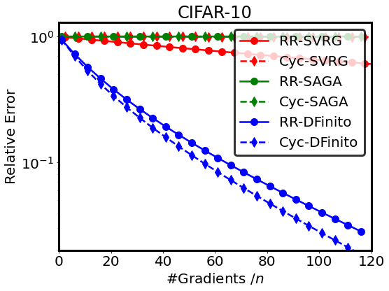
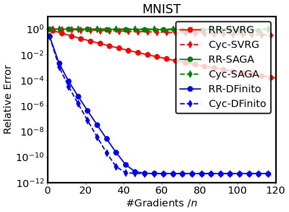
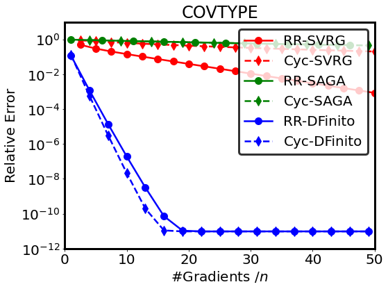
Figure 1: Comparison with SVRG and SAGA under without-replacement sampling orders using theoretical step sizes on Cifar-10 ($\lambda=0.005$), MNIST ($\lambda=0.008$), and Covtype ($\lambda=0.05$). The $y$-axis indicates the relative mean-square error $(\mathbb{E})\|x-x^{\star}\|^{2}/\|x^{0}-x^{\star}\|^{2}$ versus $\#$gradient evaluations$/n$.

5.2 DFinito with cyclic sampling

Justification of the optimal cyclic sampling order. To justify the optimal cyclic sampling order $\pi^{\star}$ suggested in Proposition 4, we test DFinito with eight arbitrarily-selected cyclic orders, and compare them with the optimal cyclic ordering $\pi^{\star}$ as well as the adaptive importance reshuffling method (Algorithm 2). To make the comparison distinguishable, we construct a least square problem with heterogeneous data samples with $n=200$, $d=50$, $L=100$, $\mu=10^{-2}$ (see Appendix I for the constructed problem). The constructed problem is with $\rho=\|{\boldsymbol{z}}^{0}-{\boldsymbol{z}}^{\star}\|^{2}_{\pi^{*}}/\|{\boldsymbol{z}}^{0}-{\boldsymbol{z}}^{\star}\|^{2}_{2}=0.006$ when $z_{i}^{0}=0$, $x^{0}=0$, and $\alpha=\frac{1}{3L}$, which is close to $1/n=0.005$. In the left plot in Fig. 2, it is observed that the optimal cyclic sampling achieves the fastest convergence rate. Furthermore, the adaptive shuffling method can match with the optimal cyclic ordering. These observations are consistent with our theoretical results derived in Sec. 4.2 and 4.3.

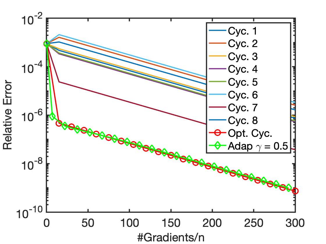
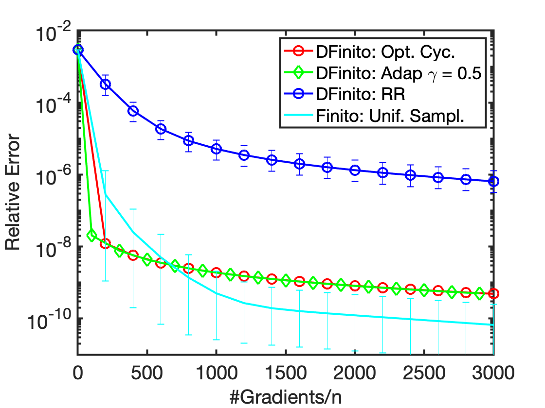
Figure 2: Left: Performance of DFinito under different sampling orders. Error metric: $\|x-x^{\star}\|^{2}/\|x^{0}-x^{\star}\|^{2}$. Right: Comparison of DFinito under $\pi^{\star}$-cyclic sampling and uniform sampling in a highly heterogeneous scenario. Error metric: $\|\nabla F(x)\|^{2}/\|\nabla F(x^{0})\|^{2}$.

Optimal cyclic sampling can achieve sample-size-independent complexity. It is established in [26] that Finito with uniform-iid-sampling can achieve $n$-independent gradient complexity with $\alpha=\frac{n}{8L}$. In this experiment, we compare DFinito ($\alpha=\frac{2}{L}$) with Finito under uniform sampling (8 runs, $\alpha=\frac{n}{8L}$) in a convex and highly heterogeneous scenario ($\rho={\mathcal{O}}(\frac{1}{n})$). The constructed problem is with $n=500$, $d=20$, $L=0.3$, $\theta=0.5$ and $\|z_{i}^{0}-z_{i}^{\star}\|=10000*0.1^{i-1}$, $1\leq i\leq n$ (see detailed initialization in Appendix J). We also depict DFinito with random-reshuffling (8 runs) as another baseline. In the right plot of Figure 2, it is observed that the convergence curve of DFinito with $\pi^{\star}$-cyclic sampling matches with Finito with uniform sampling. This implies DFinito can achieve the same $n$-independent gradient complexity as Finito with uniform sampling.

5.3 More experiments

We conduct more experiments in Appendix J. First, we compare DFinito with GD/SGD to justify its empirical superiority to these methods. Second, we validate how different data heterogeneity will influence optimal cyclic sampling. Third, we examine the performance of SVRG, SAGA, and DFinito under without/with-replacement sampling using grid-search (not theoretical) step sizes.

6 Conclusion and Discussion

This paper develops Prox-DFinito and analyzes its convergence rate under without-replacement sampling in both convex and strongly convex scenarios. Our derived rates are state-of-the-art compared to existing results. In particular, this paper derives the best-case convergence rate for Prox-DFinito with cyclic sampling, which can be sample-size-independent in the highly data-heterogeneous scenario. A future direction is to close the gap in gradient complexity between variance reduction under without-replacement and uniform-iid-sampling in the more general setting.

Appendix

Appendix A Efficient Implementation of Prox-Finito

Algorithm 3 Prox-Finito: Efficient Implementation

  Input: $\bar{z}^{0}=\frac{1}{n}\sum\limits_{i=1}^{n}z_{i}^{0}$, step-size $\alpha$, and $\theta\in(0,1)$;

  for epoch $k=0,1,2,\cdots$ do

     for iteration $t=kn+1,kn+2,\cdots,(k+1)n$ do

        $x^{t-1}={\mathbf{prox}}_{\alpha r}(\bar{z}^{t-1})$;

        Pick $i_{t}$ with some rule;

        Compute $d_{i_{t}}^{t}=x^{t-1}-\alpha\nabla f_{i}(x^{t-1})-z_{i_{t}}^{t-1}$;

        Update $\bar{z}^{t}=\bar{z}^{t-1}+d_{i_{t}}^{t}/n$;

        Update $z_{i_{t}}^{t}=z_{i_{t}}^{t-1}+\theta d_{i_{t}}^{t}$ and delete $d_{i_{t}}^{t}$;

     end for

     $\bar{z}^{(k+1)n}\leftarrow(1-\theta)\bar{z}^{kn}+\theta\bar{z}^{(k+1)n}$;

  end for

Appendix B Operator’s Form

B.1 Proof of Proposition 1

Proof.

In fact, it suffices to notice that

$${\boldsymbol{z}}^{kn+\ell}=\begin{cases}{\mathcal{T}}_{\pi(\ell)}{\boldsymbol{z}}^{kn+\ell-1}&\mbox{if $\ell\in[n-1]$}\\ (1-\theta){\boldsymbol{z}}^{kn}+{\mathcal{T}}_{\pi(n)}{\boldsymbol{z}}^{kn+n-1}&\mbox{if $\ell=n$},\end{cases}$$

and the $x$-update in (7) directly follows (4d). ∎

B.2 Proof of Proposition 3

Proof.

With definition (2), we can reach the following important relation:

$$x={\mathbf{prox}}_{\alpha r}(y)\,\Longleftrightarrow\,0\in\alpha\,\partial\,r(x)+x-y.$$ (23)

Sufficiency. Assuming $x^{\star}$ minimizes $F(z)+r(x)$, it holds that $0\in\nabla F(x^{\star})+\partial\,r(x^{\star})$. Let $z_{i}^{\star}=(I-\alpha\nabla f_{i})(x^{\star})$ and ${\boldsymbol{z}}^{\star}=\mbox{col}\{z_{1}^{\star},\dots,z_{n}^{\star}\}$, we now prove ${\boldsymbol{z}}^{\star}$ satisfies (9) and (10).

Note ${\mathcal{A}}{\boldsymbol{z}}^{\star}=\frac{1}{n}\sum\limits_{i=1}^{n}(I-\alpha\nabla f_{i})(x^{\star})=x^{\star}-\alpha\nabla F(x^{\star})$ and $0\in x^{\star}-(x^{\star}-\alpha\nabla F(x^{\star}))+\alpha\,\partial\,r(x^{\star})$, it holds that

$$x^{\star}={\mathbf{prox}}_{\alpha r}(x^{\star}-\alpha\nabla F(x^{\star}))={\mathbf{prox}}_{\alpha r}({\mathcal{A}}{\boldsymbol{z}}^{\star})$$ (24)

and hence

$$(I-\alpha\nabla f_{i})\circ{\mathbf{prox}}_{\alpha r}({\mathcal{A}}{\boldsymbol{z}}^{\star})=(I-\alpha\nabla f_{i})(x^{\star})=z_{i}^{\star},\quad\forall\,i\in[n].$$ (25)

Therefore, ${\boldsymbol{z}}^{\star}$ satisfies (9) and (10).

Necessity. Assuming ${\boldsymbol{z}}^{\star}={\mathcal{T}}_{i}{\boldsymbol{z}}^{\star},\,\forall\,i\in[n]$, we have $z_{i}^{\star}=(I-\alpha\nabla f_{i})\circ{\mathbf{prox}}_{\alpha r}({\mathcal{A}}{\boldsymbol{z}}^{\star})$. By averaging all $z_{i}^{\star}$, we have

$${\mathcal{A}}{\boldsymbol{z}}^{\star}=(I-\alpha\nabla F)\circ{\mathbf{prox}}_{\alpha r}({\mathcal{A}}{\boldsymbol{z}}^{\star}).$$ (26)

Let $x^{\star}={\mathbf{prox}}_{\alpha r}({\mathcal{A}}{\boldsymbol{z}}^{\star})$ and apply ${\mathbf{prox}}_{\alpha r}$ to (26), we reach

$$x^{\star}={\mathbf{prox}}_{\alpha r}(x^{\star}-\alpha\nabla F(x^{\star})),$$ (27)

which indicates $0\in\alpha\,\partial\,r(x^{\star})+x^{\star}-(x^{\star}-\alpha F(x^{\star}))\,\Longleftrightarrow\,0\in\nabla F(x^{\star})+\partial\,r(x^{\star})$, i.e. $x^{\star}$ is a minimizer. ∎

Appendix C Cyclic–Convex

C.1 Proof of Lemma 1

Proof.

Without loss of generality, we only prove the case in which $\pi=(1,2,\dots,n)$ where ${\mathcal{T}}_{\pi}={\mathcal{T}}_{n}\circ\cdots\circ{\mathcal{T}}_{2}\circ{\mathcal{T}}_{1}$.

To ease the notation, for ${\boldsymbol{z}}\in\mathbb{R}^{nd}$, we define $h_{i}$-norm as

$$\|{\boldsymbol{z}}\|_{h_{i}}^{2}=\frac{1}{n}\sum\limits_{j=1}^{n}\big{(}\mbox{mod}_{n}(j-i-1)+1\big{)}\|z_{j}\|^{2}.$$ (28)

Note $\|{\boldsymbol{z}}\|_{h_{n}}^{2}=\|{\boldsymbol{z}}\|_{h_{0}}^{2}=\|{\boldsymbol{z}}\|_{\pi}^{2}$ when $\pi=(1,2,\dots,n)$.

To begin with, we introduce the non-expansiveness of operator $(I-\alpha\nabla f_{i})\circ{\mathbf{prox}}_{\alpha r}$, i.e.

$$\|(I-\alpha\nabla f_{i})\circ{\mathbf{prox}}_{\alpha r}(x)-(I-\alpha\nabla f_{i})\circ{\mathbf{prox}}_{\alpha r}(y)\|^{2}\leq\|x-y\|^{2},\,\forall\,x,y\in\mathbb{R}^{d}\mbox{ and }i\in[n].$$ (29)

Note that ${\mathbf{prox}}_{\alpha r}$ is non-expansive by itself; see [30, 13]. $I-\alpha\nabla f_{i}$ is non-expansive because

$$\ \|x-\alpha\nabla f_{i}(x)-y+\alpha\nabla f_{i}(y)\|^{2}$$

$$= \ \|x-y\|^{2}-2\alpha\langle x-y,\nabla f_{i}(x)-\nabla f_{i}(y)\rangle+\alpha^{2}\|\nabla f_{i}(x)-\nabla f_{i}(y)\|^{2}$$

$$\leq \ \|x-y\|^{2}-\Big{(}\frac{2\alpha}{L}-\alpha^{2}\Big{)}\|\nabla f_{i}(x)-\nabla f_{i}(y)\|^{2}$$

$$\leq \ \|x-y\|^{2}\quad\forall x\in\mathbb{R}^{d},y\in\mathbb{R}^{d}$$

where the last inequality holds when $\alpha\leq\frac{2}{L}$. Therefore, the non-expansiveness of $I-\alpha\nabla f_{i}$ and ${\mathbf{prox}}_{\alpha r}$ imply that the composition $(I-\alpha\nabla f_{i})\circ{\mathbf{prox}}_{\alpha r}$ is also non-expansive.

We then check the operator ${\mathcal{T}}_{i}$. Suppose ${\boldsymbol{u}}\in\mathbb{R}^{nd}$ and ${\boldsymbol{v}}\in\mathbb{R}^{nd}$,

$$\begin{split}\|{\mathcal{T}}_{i}{\boldsymbol{u}}-{\mathcal{T}}_{i}{\boldsymbol{v}}\|^{2}_{h_{i}}=&\ \frac{1}{n}\sum_{j\neq i}\big{(}\mbox{mod}_{n}(j-i-1)+1\big{)}\|u_{j}-v_{j}\|^{2}\\ &\quad+\|(I-\alpha\nabla f_{i})\circ{\mathbf{prox}}_{\alpha r}({\mathcal{A}}{\boldsymbol{u}})-(I-\alpha\nabla f_{i})\circ{\mathbf{prox}}_{\alpha r}({\mathcal{A}}{\boldsymbol{v}})\|^{2}\\ \overset{(a)}{\leq}&\ \frac{1}{n}\sum_{j\neq i}\big{(}\mbox{mod}_{n}(j-i-1)+1\big{)}\|u_{j}-v_{j}\|^{2}+\|{\mathcal{A}}{\boldsymbol{u}}-{\mathcal{A}}{\boldsymbol{v}}\|^{2}\\ \overset{(b)}{\leq}&\ \frac{1}{n}\sum_{j\neq i}\big{(}\mbox{mod}_{n}(j-i-1)+1\big{)}\|u_{j}-v_{j}\|^{2}+\frac{1}{n}\sum_{j=1}^{n}\|u_{j}-v_{j}\|^{2}\\ =&\ \frac{1}{n}\sum_{j=1}^{n}\big{(}\mbox{mod}_{n}(j-i)+1\big{)}\|u_{j}-v_{j}\|^{2}=\|{\boldsymbol{u}}-{\boldsymbol{v}}\|_{h_{i-1}}^{2}.\end{split}$$ (30)

In the above inequalities, the inequality (a) holds due to (29) and (b) holds because

$$\|{\mathcal{A}}{\boldsymbol{u}}-{\mathcal{A}}{\boldsymbol{v}}\|^{2}=\|\frac{1}{n}\sum_{i=1}^{n}(u_{i}-v_{i})\|^{2}\leq\frac{1}{n}\sum_{i=1}^{n}\|u_{i}-v_{i}\|^{2}.$$ (31)

With inequality (30), we have that

$$\begin{split}\|{\mathcal{T}}_{\pi}{\boldsymbol{u}}-{\mathcal{T}}_{\pi}{\boldsymbol{v}}\|^{2}_{\pi}=&\ \|{\mathcal{T}}_{n}{\mathcal{T}}_{n-1}\cdots{\mathcal{T}}_{1}{\boldsymbol{u}}-{\mathcal{T}}_{n}{\mathcal{T}}_{n-1}\cdots{\mathcal{T}}_{1}{\boldsymbol{v}}\|^{2}_{h_{n}}\\ \leq&\ \|{\mathcal{T}}_{n-1}\cdots{\mathcal{T}}_{1}{\boldsymbol{u}}-{\mathcal{T}}_{n-1}\cdots{\mathcal{T}}_{1}{\boldsymbol{v}}\|^{2}_{h_{n-1}}\\ \leq&\ \|{\mathcal{T}}_{n-2}\cdots{\mathcal{T}}_{1}{\boldsymbol{u}}-{\mathcal{T}}_{n-2}\cdots{\mathcal{T}}_{1}{\boldsymbol{v}}\|^{2}_{h_{n-2}}\\ \leq&\ \cdots\\ \leq&\ \|{\mathcal{T}}_{1}{\boldsymbol{u}}-{\mathcal{T}}_{1}{\boldsymbol{v}}\|^{2}_{h_{1}}\\ \leq&\ \|{\boldsymbol{u}}-{\boldsymbol{v}}\|^{2}_{h_{0}}=\|{\boldsymbol{u}}-{\boldsymbol{v}}\|^{2}_{\pi}.\end{split}$$ (32)

∎

C.2 Proof of Lemma 2

Proof.

We define ${\mathcal{S}}_{\pi}=(1-\theta)I+\theta{\mathcal{T}}_{\pi}$ to ease the notation. Then ${\boldsymbol{z}}^{(k+1)n}={\mathcal{S}}_{\pi}{\boldsymbol{z}}^{kn}$ by Proposition 1. To prove Lemma 2, notice that $\forall\ k=1,2,\cdots$

$$\|{\boldsymbol{z}}^{(k+1)n}-{\boldsymbol{z}}^{kn}\|^{2}_{\pi} =\|{\mathcal{S}}_{\pi}{\boldsymbol{z}}^{kn}-{\mathcal{S}}_{\pi}{\boldsymbol{z}}^{(k-1)n}\|^{2}_{\pi}$$

$$\leq(1-\theta)\|{\boldsymbol{z}}^{kn}-{\boldsymbol{z}}^{(k-1)n}\|^{2}_{\pi}+\theta\|{\mathcal{T}}_{\pi}{\boldsymbol{z}}^{kn}-{\mathcal{T}}_{\pi}{\boldsymbol{z}}^{(k-1)n}\|^{2}_{\pi}$$

$$\overset{\eqref{xnsdbbb}}{\leq}\|{\boldsymbol{z}}^{kn}-{\boldsymbol{z}}^{(k-1)n}\|^{2}_{\pi}$$ (33)

The above relation implies that $\|{\boldsymbol{z}}^{(k+1)n}-{\boldsymbol{z}}^{kn}\|^{2}_{\pi}$ is non-increasing. Next,

$$\|{\boldsymbol{z}}^{(k+1)n}-{\boldsymbol{z}}^{\star}\|^{2}_{\pi} \overset{}{=}\|(1-\theta){\boldsymbol{z}}^{kn}+\theta{\mathcal{T}}_{\pi}({\boldsymbol{z}}^{kn})-{\boldsymbol{z}}^{\star}\|^{2}_{\pi}$$

$$=(1-\theta)\|{\boldsymbol{z}}^{kn}-{\boldsymbol{z}}^{\star}\|^{2}_{\pi}+\theta\|{\mathcal{T}}_{\pi}({\boldsymbol{z}}^{kn})-{\boldsymbol{z}}^{\star}\|^{2}_{\pi}-\theta(1-\theta)\|{\boldsymbol{z}}^{kn}-{\mathcal{T}}({\boldsymbol{z}}^{kn})\|^{2}_{\pi}$$

$$\overset{(c)}{\leq}\|{\boldsymbol{z}}^{kn}-{\boldsymbol{z}}^{\star}\|^{2}_{\pi}-\theta(1-\theta)\|{\boldsymbol{z}}^{kn}-{\mathcal{T}}_{\pi}({\boldsymbol{z}}^{kn})\|^{2}_{\pi}$$

$$=\|{\boldsymbol{z}}^{kn}-{\boldsymbol{z}}^{\star}\|^{2}_{\pi}-\frac{1-\theta}{\theta}\|{\boldsymbol{z}}^{kn}-{\mathcal{S}}_{\pi}({\boldsymbol{z}}^{kn})\|^{2}_{\pi}$$

$$=\|{\boldsymbol{z}}^{kn}-{\boldsymbol{z}}^{\star}\|^{2}_{\pi}-\frac{1-\theta}{\theta}\|{\boldsymbol{z}}^{kn}-{\boldsymbol{z}}^{(k+1)n}\|^{2}_{\pi}.$$ (34)

where equality (c) holds because Proposition 3 implies ${\mathcal{T}}_{\pi}{\boldsymbol{z}}^{\star}={\boldsymbol{z}}^{\star}$.

Summing the above inequality from $0$ to $k$ we have

$$\|{\boldsymbol{z}}^{(k+1)n}-{\boldsymbol{z}}^{\star}\|^{2}_{\pi}\leq\|{\boldsymbol{z}}^{0}-{\boldsymbol{z}}^{\star}\|^{2}_{\pi}-\frac{1-\theta}{\theta}\sum_{\ell=0}^{k}\|{\boldsymbol{z}}^{\ell n}-{\boldsymbol{z}}^{(\ell+1)n}\|^{2}_{\pi}.$$ (35)

Since $\|{\boldsymbol{z}}^{(k+1)n}-{\boldsymbol{z}}^{kn}\|^{2}_{\pi}$ is non-increasing, we reach the conclusion. ∎

C.3 Proof of Theorem 1

Proof.

Since $z_{\pi(j)}^{kn+j-1}=z_{\pi(j)}^{kn}$ for $1\leq j\leq n$, it holds that

$$\begin{split}\bar{z}^{(k+1)n}&=(1-\theta)\bar{z}^{kn}+\theta\left(\bar{z}^{kn}+\sum\limits_{j=1}^{n}\frac{1}{n}\left((I-\alpha\nabla f_{\pi(j)})(x^{kn+j-1})-z_{\pi(j)}^{kn+j-1}\right)\right)\\ &=(1-\theta)\bar{z}^{kn}+\theta\left(\bar{z}^{kn}+\sum\limits_{j=1}^{n}\frac{1}{n}\left((I-\alpha\nabla f_{\pi(j)})(x^{kn+j-1})-z_{\pi(j)}^{kn}\right)\right)\\ &=(1-\theta)\bar{z}^{kn}+\theta\sum\limits_{j=1}^{n}\frac{1}{n}(I-\alpha\nabla f_{\pi(j)})(x^{kn+j-1}),\end{split}$$ (36)

which further implies that

$$\frac{1}{n}\sum\limits_{j=1}^{n}\nabla f_{\pi(j)}(x^{kn+j-1})=\frac{1}{\theta\alpha}(\bar{z}^{kn}-\bar{z}^{(k+1)n})+\frac{1}{n\alpha}\sum\limits_{j=1}^{n}(x^{kn+j-1}-\bar{z}^{kn}).$$ (37)

As a result, we achieve

$$\begin{split}&\nabla F(x^{kn})=\frac{1}{n}\sum\limits_{j=1}^{n}\nabla f_{\pi(j)}(x^{kn})\\ =&\frac{1}{n}\sum\limits_{j=1}^{n}\left(\nabla f_{\pi(j)}(x^{kn})-\nabla f_{\pi(j)}(x^{kn+j-1})\right)+\frac{1}{n}\sum\limits_{j=1}^{n}\nabla f_{\pi(j)}(x^{kn+j-1})\\ =&\frac{1}{n}\sum\limits_{j=1}^{n}\left(\nabla f_{\pi(j)}(x^{kn})-\nabla f_{\pi(j)}(x^{kn+j-1})\right)+\frac{1}{\theta\alpha}(\bar{z}^{kn}-\bar{z}^{(k+1)n})+\frac{1}{n\alpha}\sum\limits_{j=1}^{n}(x^{kn+j-1}-\bar{z}^{kn})\\ =&\frac{1}{n\alpha}\sum\limits_{j=1}^{n}\left((I-\alpha\nabla f_{\pi(j)})(x^{kn+j-1})-(I-\alpha\nabla f_{\pi(j)})(x^{kn})\right)\\ &\quad+\frac{1}{\theta\alpha}(\bar{z}^{kn}-\bar{z}^{(k+1)n})+\frac{1}{\alpha}(x^{kn}-\bar{z}^{kn}).\end{split}$$ (38)

Notice that

$$\begin{split}&x^{kn}={\mathbf{prox}}_{\alpha r}(\bar{z}^{kn})\\ \Longleftrightarrow\,&0\in\alpha\,\partial\,r(x^{kn})+(x^{kn}-\bar{z}^{kn})\\ \Longleftrightarrow\,&\frac{1}{\alpha}(\bar{z}^{kn}-x^{kn})\triangleq\tilde{\nabla}r(x^{kn})\in\partial\,r(x^{kn}),\end{split}$$ (39)

relation (38) can be rewritten as

$$\begin{split}&\nabla F(x^{kn})+\tilde{\nabla}r(x^{kn})\\ =&\frac{1}{n\alpha}\sum\limits_{j=1}^{n}\left((I-\alpha\nabla f_{\pi(j)})(x^{kn+j-1})-(I-\alpha\nabla f_{\pi(j)})(x^{kn})\right)+\frac{1}{\theta\alpha}(\bar{z}^{kn}-\bar{z}^{(k+1)n}).\end{split}$$ (40)

Next we bound the two terms on the right hand side of (40) by $\|{\boldsymbol{z}}^{(k+1)n}-{\boldsymbol{z}}^{kn}\|^{2}_{\pi}$. For the second term, it is easy to see

$$\begin{split}\|\frac{1}{\theta\alpha}(\bar{z}^{kn}-\bar{z}^{(k+1)n})\|^{2}&=\frac{1}{n^{2}\theta^{2}\alpha^{2}}\|\sum\limits_{j=1}^{n}z_{\pi(j)}^{kn}-z_{\pi(j)}^{(k+1)n}\|^{2}\\ &\overset{(d)}{\leq}\frac{1}{n^{2}\theta^{2}\alpha^{2}}(\sum\limits_{j=1}^{n}\frac{n}{j})(\sum\limits_{j=1}^{n}\frac{j}{n}\|z_{\pi(j)}^{kn}-z_{\pi(j)}^{(k+1)n}\|^{2})\\ &\overset{(e)}{\leq}\frac{\log(n)+1}{n\theta^{2}\alpha^{2}}\|{\boldsymbol{z}}^{kn}-{\boldsymbol{z}}^{(k+1)n}\|_{\pi}^{2},\end{split}$$ (41)

where inequality (d) is due to Cauchy’s inequality $(\sum\limits_{j=1}^{n}a_{j})^{2}\leq\sum\limits_{j=1}^{n}\frac{1}{\beta_{j}}\sum\limits_{j=1}^{n}\beta_{j}a_{j}^{2}$ with $\beta_{j}>0$, $\forall\,j\in[n]$ and inequality (e) holds because $\sum\limits_{j=1}^{n}\frac{1}{j}\leq\log(n)+1$.

For the first term, we first note for $2\leq j\leq n$,

$$z_{\pi(\ell)}^{kn+j-1}=\begin{cases}z_{\pi(\ell)}^{kn}+\frac{1}{\theta}(z_{\pi(\ell)}^{(k+1)n}-z_{\pi(\ell)}^{kn}),\quad\text{$1\leq\ell\leq j-1$};\\ z_{\pi(\ell)}^{kn},\quad\text{$\ell>j-1$}.\end{cases}$$ (42)

By (29), we have

$$\begin{split}&\|(I-\alpha\nabla f_{\pi(j)})(x^{kn+j-1})-(I-\alpha\nabla f_{\pi(j)})(x^{kn})\|^{2}\\ =&\|(I-\alpha\nabla f_{\pi(j)})\circ{\mathbf{prox}}_{\alpha r}(\bar{z}^{kn+j-1})-(I-\alpha\nabla f_{\pi(j)})\circ{\mathbf{prox}}_{\alpha r}(\bar{z}^{kn})\|^{2}\\ \leq&\|\bar{z}^{kn+j-1}-\bar{z}^{kn}\|^{2}=\|\frac{1}{n}\sum\limits_{\ell=1}^{n}(z_{\pi(\ell)}^{kn+j-1}-z_{\pi(\ell)}^{kn})\|^{2}\\ =&\frac{1}{n^{2}\theta^{2}}\|\sum\limits_{\ell=1}^{j-1}(z_{\pi(\ell)}^{(k+1)n}-z_{\pi(\ell)}^{kn})\|^{2}\leq\frac{1}{n^{2}\theta^{2}}\sum\limits_{\ell=1}^{j-1}\frac{n}{\ell}\sum\limits_{\ell=1}^{j-1}\frac{\ell}{n}\|z_{\pi(\ell)}^{(k+1)n}-z_{\pi(\ell)}^{kn}\|^{2}\\ \leq&\frac{\log(n)+1}{n\theta^{2}}\|{\boldsymbol{z}}^{(k+1)n}-{\boldsymbol{z}}^{kn}\|_{\pi}^{2}.\end{split}$$ (43)

In the last inequality, we used the algebraic inequality that $\sum\limits_{\ell=1}^{n}\frac{1}{\ell}\leq\log(n)+1$. Therefore we have

$$\|\frac{1}{n\alpha}\sum\limits_{j=1}^{n}\left((I-\alpha\nabla f_{\pi(j)})(x^{kn+j-1})-(I-\alpha\nabla f_{\pi(j)})(x^{kn})\right)\|^{2}$$

$$= \frac{1}{n^{2}\alpha^{2}}\|\sum\limits_{j=2}^{n}\left((I-\alpha\nabla f_{\pi(j)})(x^{kn+j-1})-(I-\alpha\nabla f_{\pi(j)})(x^{kn})\right)\|^{2}$$

$$\leq \frac{1}{n^{2}\alpha^{2}}(n-1)^{2}\frac{\log(n)+1}{n\theta^{2}}\|{\boldsymbol{z}}^{(k+1)n}-{\boldsymbol{z}}^{kn}\|_{\pi}^{2}$$

$$\leq \frac{\log(n)+1}{n\theta^{2}\alpha^{2}}\|{\boldsymbol{z}}^{kn}-{\boldsymbol{z}}^{(k+1)n}\|_{\pi}^{2}.$$ (44)

Combining (41) and (C.3), we immediately obtain

$$\min\limits_{g\in\partial\,r(x^{kn})}\|\nabla F(x^{kn})+g\|^{2}\leq\|\nabla F(x^{kn})+\tilde{\nabla}r(x^{kn})\|^{2}$$

$$\leq 2(\|\frac{1}{n\alpha}\sum\limits_{j=1}^{n}\left((I-\alpha\nabla f_{\pi(j)})(x^{kn+j-1})-(I-\alpha\nabla f_{\pi(j)})(x^{kn})\right)\|^{2}+\|\frac{1}{\theta\alpha}(\bar{z}^{kn}-\bar{z}^{(k+1)n})\|^{2})$$

$$\leq 2(\frac{\log(n)+1}{n\theta^{2}\alpha^{2}}\|{\boldsymbol{z}}^{kn}-{\boldsymbol{z}}^{(k+1)n}\|_{\pi}^{2}+\frac{\log(n)+1}{n\theta^{2}\alpha^{2}}\|{\boldsymbol{z}}^{kn}-{\boldsymbol{z}}^{(k+1)n}\|_{\pi}^{2})$$

$$= \left(\frac{2}{\alpha L}\right)^{2}\frac{(\log(n)+1)L^{2}}{n\theta^{2}}\|{\boldsymbol{z}}^{kn}-{\boldsymbol{z}}^{(k+1)n}\|_{\pi}^{2}$$

$$\leq \left(\frac{2}{\alpha L}\right)^{2}\frac{L^{2}}{\theta(1-\theta)(k+1)}\frac{\log(n)+1}{n}\|{\boldsymbol{z}}^{0}-{\boldsymbol{z}}^{\star}\|_{\pi}^{2}.$$ (45)

∎

Appendix D RR–Convex

D.1 Non-expansiveness Lemma for RR

While replacing order-specific norm with standard $\ell_{2}$ norm. the following lemma establishes that ${\mathcal{T}}_{\tau_{k}}$ is non-expansive in expectation.

Lemma 3.

Under Assumption 1, if step-size $0<\alpha\leq\frac{2}{L}$ and data is sampled with random reshuffling, it holds that

$$\mathbb{E}_{\tau_{k}}\|{\mathcal{T}}_{\tau_{k}}{\boldsymbol{u}}-{\mathcal{T}}_{\tau_{k}}{\boldsymbol{v}}\|^{2}\leq\|{\boldsymbol{u}}-{\boldsymbol{v}}\|^{2}.$$ (46)

It is worth noting that inequality (46) holds for $\ell_{2}$-norm rather than the order-specific norm due to the randomness brought by random reshuffling.

Proof.

Given any vector $h=[\,h(1),\,h(2),\cdots,\,h(n)\,]^{T}\in\mathbb{R}^{n}$ with positive elements where $h_{i}$ denotes the $i$-th element of $h$, define $h$-norm as follows

$$\|{\boldsymbol{z}}\|^{2}_{h}=\sum\limits_{i=1}^{n}h(i)\|z_{i}\|^{2}$$ (47)

for any ${\boldsymbol{z}}=\mbox{col}\{z_{1},z_{2},\cdots,z_{n}\}\in\mathbb{R}^{nd}$. Following arguments in (30), it holds that

$$\|{\mathcal{T}}_{i}{\boldsymbol{u}}-{\mathcal{T}}_{i}{\boldsymbol{v}}\|_{h}^{2}\leq\|{\boldsymbol{u}}-{\boldsymbol{v}}\|^{2}_{h^{\prime}}$$ (48)

where $h^{\prime}=h+\frac{1}{n}h(i)\mathds{1}_{n}-h(i)e_{i}$ and $e_{i}$ is the $i$-th unit vector. Define

$$M_{i}:=I+\frac{1}{n}m_{i}e_{i}^{T}\in\mathbb{R}^{n\times n}$$ (49)

where $m_{i}=\mathds{1}_{n}-ne_{i}$, then we can summarize the above conclusion as follows.

Lemma 4.

Given $h\in\mathbb{R}^{n}$ with positive elements and its corresponding $h$-norm, under Assumption 1, if step-size $0<\alpha\leq\frac{2}{L}$, it holds that

$$\|{\mathcal{T}}_{i}{\boldsymbol{u}}-{\mathcal{T}}_{i}{\boldsymbol{v}}\|_{h}^{2}\leq\|{\boldsymbol{u}}-{\boldsymbol{v}}\|_{M_{i}h}^{2}\quad\forall\,{\boldsymbol{u}},{\boldsymbol{v}}\in\mathbb{R}^{nd}.$$ (50)

Therefore, with Lemma 4, we have that

$$\begin{split}\|{\mathcal{T}}_{\tau}{\boldsymbol{u}}-{\mathcal{T}}_{\tau}{\boldsymbol{v}}\|^{2}=&\ \|{\mathcal{T}}_{\tau(n)}{\mathcal{T}}_{\tau(n-1)}\cdots{\mathcal{T}}_{\tau(1)}{\boldsymbol{u}}-{\mathcal{T}}_{\tau(n)}{\mathcal{T}}_{\tau(n-1)}\cdots{\mathcal{T}}_{\tau(1)}{\boldsymbol{v}}\|^{2}_{\mathds{1}_{n}}\\ \leq&\ \|{\mathcal{T}}_{\tau(n-1)}\cdots{\mathcal{T}}_{\tau(1)}{\boldsymbol{u}}-{\mathcal{T}}_{\tau(n-1)}\cdots{\mathcal{T}}_{\tau(1)}{\boldsymbol{v}}\|^{2}_{M_{\tau(n)}\mathds{1}_{n}}\\ \leq&\ \|{\mathcal{T}}_{\tau(n-2)}\cdots{\mathcal{T}}_{\tau(1)}{\boldsymbol{u}}-{\mathcal{T}}_{\tau(n-2)}\cdots{\mathcal{T}}_{\tau(1)}{\boldsymbol{v}}\|^{2}_{{M_{\tau(n-1)}M_{\tau(n)}\mathds{1}_{n}}}\\ \leq&\ \cdots\\ \leq&\ \|{\mathcal{T}}_{\tau(1)}{\boldsymbol{u}}-{\mathcal{T}}_{\tau(1)}{\boldsymbol{v}}\|^{2}_{M_{\tau(2)}\cdots M_{\tau(n)}\mathds{1}_{n}}\\ \leq&\ \|{\boldsymbol{u}}-{\boldsymbol{v}}\|^{2}_{M_{\tau(1)}\cdots M_{\tau(n)}\mathds{1}_{n}}.\end{split}$$ (51)

With the above relation, if we can prove

$$\mathbb{E}_{\tau}M_{\tau(1)}\cdots M_{\tau(n)}\mathds{1}_{n}=\mathds{1}_{n},$$ (52)

then we can complete the proof by

$$\mathbb{E}_{\tau}\,\|{\mathcal{T}}_{\tau}{\boldsymbol{u}}-{\mathcal{T}}_{\tau}{\boldsymbol{v}}\|^{2}\leq\mathbb{E}_{\tau}\,\|{\boldsymbol{u}}-{\boldsymbol{v}}\|^{2}_{M_{\tau(1)}\cdots M_{\tau(n)}\mathds{1}_{n}}=\|{\boldsymbol{u}}-{\boldsymbol{v}}\|^{2}_{\mathbb{E}\,M_{\tau(1)}\cdots M_{\tau(n)}\mathds{1}_{n}}=\|{\boldsymbol{u}}-{\boldsymbol{v}}\|^{2}.$$ (53)

To prove (52), we notice that $e_{i}^{T}m_{j}=1,\forall\,i\neq j$ which leads to $m_{\tau(j_{1})}e_{\tau(j_{1})}^{T}m_{\tau(j_{2})}e_{\tau(j_{2})}^{T}\cdots m_{\tau(j_{t})}e_{\tau(j_{t})}^{T}=m_{\tau(j_{1})}e_{\tau(j_{t})}^{T}$, $\forall\,j_{1}<j_{2}<\cdots<j_{t}$. This fact further implies that

$$M_{\tau(1)}\cdots M_{\tau(n)} =(I+\frac{1}{n}m_{\tau(1)}e_{\tau(1)}^{T})\cdots(I+\frac{1}{n}m_{\tau(n)}e_{\tau(n)}^{T})$$

$$=I+\frac{1}{n}\sum\limits_{i=1}^{n}m_{i}e_{i}^{T}+\sum\limits_{t=2}^{n}\sum\limits_{j_{1}<\cdots<j_{t}}\frac{1}{n^{t}}m_{\tau(j_{1})}e_{\tau(j_{1})}^{T}\cdots m_{\tau(j_{t})}e_{\tau(j_{t})}^{T}$$

$$=I+\frac{1}{n}\sum\limits_{i=1}^{n}m_{i}e_{i}^{T}+\sum\limits_{t=2}^{n}\sum\limits_{i+t-1\leq j}\binom{j-i-1}{t-2}\frac{1}{n^{t}}m_{\tau(i)}e_{\tau(j)}^{T}$$

$$=I+\frac{1}{n}\sum\limits_{i=1}^{n}m_{i}e_{i}^{T}+\sum\limits_{i<j}\sum\limits_{t=2}^{j-i+1}\binom{j-i-1}{t-2}\frac{1}{n^{t}}m_{\tau(i)}e_{\tau(j)}^{T}$$

$$=I+\frac{1}{n}\sum\limits_{i=1}^{n}m_{i}e_{i}^{T}+\sum\limits_{i<j}m_{\tau(i)}e_{\tau(j)}^{T}\frac{1}{n^{2}}(1+\frac{1}{n})^{j-i-1}.$$ (54)

It is easy to verify $\sum\limits_{i=1}^{n}m_{i}e_{i}^{T}\mathds{1}_{n}=0$ and

$$\begin{split}\mathbb{E}_{\tau}\,m_{\tau(i)}e_{\tau(j)}^{T}\mathds{1}_{n}&=\frac{1}{n(n-1)}\sum\limits_{i\neq j}m_{i}e_{j}^{T}\mathds{1}_{n}\\ &=\frac{1}{n(n-1)}\left(\left(\sum\limits_{i=1}^{n}m_{i}\right)\left(\sum\limits_{j=1}^{n}e_{j}\right)^{T}-\sum\limits_{i=1}^{n}m_{i}e_{i}^{T}\right)\mathds{1}_{n}=0.\end{split}$$ (55)

We can prove (52) by combining (D.1) and (55). ∎

D.2 Proof of Theorem 2

Proof.

In fact, with similar arguments of Appendix C.2 and noting ${\mathcal{T}}_{\tau}{\boldsymbol{z}}^{\star}={\boldsymbol{z}}^{\star}$ for any realization of $\tau$, we can achieve

Lemma 5.

Under Assumption 1, if step-size $0<\alpha\leq\frac{2}{L}$ and the data is sampled with random reshuffling, it holds for any $k=0,1,\cdots$ that

$$\mathbb{E}\,\|{\boldsymbol{z}}^{(k+1)n}-{\boldsymbol{z}}^{kn}\|^{2}\leq\frac{\theta}{(k+1)(1-\theta)}\|{\boldsymbol{z}}^{0}-{\boldsymbol{z}}^{\star}\|^{2}.$$ (56)

Based on Lemma (5), we are now able to prove Theorem 2. By arguments similar to Appendix C.3, $\exists\,\tilde{\nabla}r(x^{kn})=\frac{1}{\alpha}(\bar{z}^{kn}-x^{kn})\in\partial\,r(x^{kn})$ such that

$$\begin{split}&\nabla F(x^{kn})+\tilde{\nabla}r(x^{kn})\\ =&\frac{1}{n\alpha}\sum\limits_{j=1}^{n}\left((I-\alpha\nabla f_{\tau_{k}(j)})(x^{kn+j-1})-(I-\alpha\nabla f_{\tau_{k}(j)})(x^{kn})\right)+\frac{1}{\theta\alpha}(\bar{z}^{kn}-\bar{z}^{(k+1)n}).\end{split}$$ (57)

The second term on the right-hand-side of (57) can be bounded as

$$\|\frac{1}{\theta\alpha}(\bar{z}^{kn}-\bar{z}^{(k+1)n})\|=\frac{1}{n^{2}\theta^{2}\alpha^{2}}\|\sum\limits_{j=1}^{n}z_{j}^{kn}-z_{j}^{(k+1)n}\|^{2}\leq\frac{1}{n\theta^{2}\alpha^{2}}\|{\boldsymbol{z}}^{kn}-{\boldsymbol{z}}^{(k+1)n}\|^{2}.$$ (58)

To bound the first term, it is noted that $2\leq j\leq n$,

$$z_{\tau_{k}(\ell)}^{kn+j-1}=\begin{cases}z_{\tau_{k}(\ell)}^{kn}+\frac{1}{\theta}(z_{\tau_{k}(\ell)}^{(k+1)n}-z_{\tau_{k}(\ell)}^{kn}),\quad\text{$1\leq\ell\leq j-1$};\\ z_{\tau_{k}(\ell)}^{kn},\quad\text{$\ell>j-1$}.\end{cases}$$ (59)

By (29), we have

$$\begin{split}&\|(I-\alpha\nabla f_{\tau_{k}(j)})(x^{kn+j-1})-(I-\alpha\nabla f_{\tau_{k}(j)})(x^{kn})\|^{2}\\ =&\|(I-\alpha\nabla f_{\tau_{k}(j)})\circ{\mathbf{prox}}_{\alpha r}(\bar{z}^{kn+j-1})-(I-\alpha\nabla f_{\tau_{k}(j)})\circ{\mathbf{prox}}_{\alpha r}(\bar{z}^{kn})\|^{2}\\ \leq&\|\bar{z}^{kn+j-1}-\bar{z}^{kn}\|^{2}=\|\frac{1}{n}\sum\limits_{\ell=1}^{n}(z_{\ell}^{kn+j-1}-z_{\ell}^{kn})\|^{2}\\ =&\frac{1}{n^{2}\theta^{2}}\|\sum\limits_{\ell=1}^{j-1}(z_{\ell}^{(k+1)n}-z_{\ell}^{kn})\|^{2}\leq\frac{j-1}{n^{2}\theta^{2}}\sum\limits_{\ell=1}^{j-1}\|z_{\ell}^{(k+1)n}-z_{\ell}^{kn}\|^{2}\\ \leq&\frac{j-1}{n^{2}\theta^{2}}\|{\boldsymbol{z}}^{(k+1)n}-{\boldsymbol{z}}^{kn}\|^{2}.\end{split}$$ (60)

Therefore we have

$$\|\frac{1}{n\alpha}\sum\limits_{j=1}^{n}\left((I-\alpha\nabla f_{\tau_{k}(j)})(x^{kn+j-1})-(I-\alpha\nabla f_{\tau_{k}(j)})(x^{kn})\right)\|^{2}$$

$$= \frac{1}{n^{2}\alpha^{2}}\|\sum\limits_{j=2}^{n}\left((I-\alpha\nabla f_{\tau_{k}(j)})(x^{kn+j-1})-(I-\alpha\nabla f_{\tau_{k}(j)})(x^{kn})\right)\|^{2}$$

$$= \frac{1}{n^{2}\alpha^{2}}\sum\limits_{j=2}^{n}\sqrt{j-1}\sum\limits_{j=2}^{n}\frac{1}{\sqrt{j-1}}\|\left((I-\alpha\nabla f_{\tau_{k}(j)})(x^{kn+j-1})-(I-\alpha\nabla f_{\tau_{k}(j)})(x^{kn})\right)\|^{2}$$

$$\leq \frac{1}{n^{2}\alpha^{2}}\sum\limits_{j=2}^{n}\sqrt{j-1}\sum\limits_{j=2}^{n}\frac{1}{\sqrt{j-1}}\frac{j-1}{n^{2}}\|{\boldsymbol{z}}^{(k+1)n}-{\boldsymbol{z}}^{kn}\|^{2}$$

$$\leq \frac{4}{9}\frac{1}{n\theta^{2}\alpha^{2}}\|{\boldsymbol{z}}^{(k+1)n}-{\boldsymbol{z}}^{kn}\|^{2}.$$ (61)

In the last inequality, we use the algebraic inequality that $\sum\limits_{j=2}^{n}\sqrt{j-1}\leq\int_{1}^{n}\sqrt{x}dx=\frac{2}{3}x^{\frac{3}{2}}\big{|}_{1}^{n}\leq\frac{2}{3}n^{\frac{3}{2}}$.

Combining (58) and (D.2), we immediately obtain

$$\min\limits_{g\in\partial\,r(x^{kn})}\|\nabla F(x^{kn})+g\|^{2}\leq\|\nabla F(x^{kn})+\tilde{\nabla}r(x^{kn})\|^{2}$$

$$\leq (\frac{2}{3}+1)\Big{(}\frac{3}{2}\|\frac{1}{n\alpha}\sum\limits_{j=1}^{n}\left((I-\alpha\nabla f_{\tau_{k}(j)})(x^{kn+j-1})-(I-\alpha\nabla f_{\tau_{k}(j)})(x^{kn})\right)\|^{2}$$

$$\qquad+\|\frac{1}{\theta\alpha}(\bar{z}^{kn}-\bar{z}^{(k+1)n})\|^{2}\Big{)}$$

$$\leq \frac{5}{3}(\frac{2}{3}\frac{1}{n\theta^{2}\alpha^{2}}\|{\boldsymbol{z}}^{kn}-{\boldsymbol{z}}^{(k+1)n}\|^{2}+\frac{1}{n\theta^{2}\alpha^{2}}\|{\boldsymbol{z}}^{kn}-{\boldsymbol{z}}^{(k+1)n}\|^{2})$$

$$= \left(\frac{5}{3\alpha L}\right)^{2}\frac{L^{2}}{n\theta^{2}}\|{\boldsymbol{z}}^{kn}-{\boldsymbol{z}}^{(k+1)n}\|^{2}$$

$$\leq \left(\frac{5}{3\alpha L}\right)^{2}\frac{L^{2}}{\theta(1-\theta)(k+1)}\frac{1}{n}\|{\boldsymbol{z}}^{0}-{\boldsymbol{z}}^{\star}\|^{2}.$$ (62)

∎

Appendix E Proof of Theorem 3

Proof.

Before proving Theorem 3, we establish the epoch operator ${\mathcal{S}}_{\pi}$ and ${\mathcal{S}}_{\tau}$ are contractive in the following sense:

Lemma 6.

Under Assumption 2, if step size $0<\alpha\leq\frac{2}{\mu+L}$, it holds that

$$\|{\mathcal{S}}_{\pi}{\boldsymbol{u}}-{\mathcal{S}}_{\pi}{\boldsymbol{v}}\|_{\pi}^{2}\leq\Big{(}1-\frac{2\theta\alpha\mu L}{\mu+L}\Big{)}\|{\boldsymbol{u}}-{\boldsymbol{v}}\|^{2}_{\pi}$$ (63)

$$\mathbb{E}\,\|{\mathcal{S}}_{\tau}{\boldsymbol{u}}-{\mathcal{S}}_{\tau}{\boldsymbol{v}}\|^{2}\leq\Big{(}1-\frac{2\theta\alpha\mu L}{\mu+L}\Big{)}\|{\boldsymbol{u}}-{\boldsymbol{v}}\|^{2}$$ (64)

$\forall\,{\boldsymbol{u}},\,{\boldsymbol{v}}\in\mathbb{R}^{nd}$, where $\theta\in(0,1)$ is the damping parameter.

Proof of Lemma 6.

For $\pi$-order cyclic sampling, without loss of generality, it suffices to show the case of $\pi=(1,2,\dots,n)$. To begin with, we first check the operator ${\mathcal{T}}_{i}$. Suppose ${\boldsymbol{u}},\,{\boldsymbol{v}}\in\mathbb{R}^{nd}$,

$$\|{\mathcal{T}}_{i}{\boldsymbol{u}}-{\mathcal{T}}_{i}{\boldsymbol{v}}\|^{2}_{h_{i}}$$

$$= \ \frac{1}{n}\sum_{j\neq i}\big{(}\mbox{mod}_{n}(j-i-1)+1\big{)}\|u_{j}-v_{j}\|^{2}$$

$$\quad+\|(I-\alpha\nabla f_{i})\circ{\mathbf{prox}}_{\alpha r}({\mathcal{A}}{\boldsymbol{u}})-(I-\alpha\nabla f_{i})\circ{\mathbf{prox}}_{\alpha r}({\mathcal{A}}{\boldsymbol{v}})\|^{2}$$

$$\overset{(f)}{\leq} \ \frac{1}{n}\sum_{j\neq i}\big{(}\mbox{mod}_{n}(j-i-1)+1\big{)}\|u_{j}-v_{j}\|^{2}+\Big{(}1-\frac{2\alpha\mu L}{\mu+L}\Big{)}\|{\mathcal{A}}{\boldsymbol{u}}-{\mathcal{A}}{\boldsymbol{v}}\|^{2}$$

$$\overset{}{\leq} \ \frac{1}{n}\sum_{j\neq i}\big{(}\mbox{mod}_{n}(j-i-1)+1\big{)}\|u_{j}-v_{j}\|^{2}+\frac{1}{n}\sum_{j=1}^{n}\|u_{j}-v_{j}\|^{2}-\frac{2\alpha\mu L}{\mu+L}\|{\mathcal{A}}{\boldsymbol{u}}-{\mathcal{A}}{\boldsymbol{v}}\|^{2}$$

$$= \ \frac{1}{n}\sum_{j=1}^{n}\big{(}\mbox{mod}_{n}(j-i)+1\big{)}\|u_{j}-v_{j}\|^{2}-\frac{2\alpha\mu L}{\mu+L}\|{\mathcal{A}}{\boldsymbol{u}}-{\mathcal{A}}{\boldsymbol{v}}\|^{2}$$

$$= \|{\boldsymbol{u}}-{\boldsymbol{v}}\|_{h_{i-1}}^{2}-\frac{2\alpha\mu L}{\mu+L}\|{\mathcal{A}}{\boldsymbol{u}}-{\mathcal{A}}{\boldsymbol{v}}\|^{2}.$$ (65)

where $h_{i}$-norm in the first equality is defined as (28) with $\|\,\cdot\,\|_{h_{0}}^{2}=\|\,\cdot\,\|_{h_{0}}^{2}=\|\,\cdot\,\|_{\pi}^{2}$ and inequality (f) holds because

$$\ \|x-\alpha\nabla f_{i}(x)-y+\alpha\nabla f_{i}(y)\|^{2}$$

$$= \ \|x-y\|^{2}-2\alpha\langle x-y,\nabla f_{i}(x)-\nabla f_{i}(y)\rangle+\alpha^{2}\|\nabla f_{i}(x)-\nabla f_{i}(y)\|^{2}$$

$$\leq \ \Big{(}1-\frac{2\alpha\mu L}{\mu+L}\Big{)}\|x-y\|^{2}-\Big{(}\frac{2\alpha}{\mu+L}-\alpha^{2}\Big{)}\|\nabla f_{i}(x)-\nabla f_{i}(y)\|^{2}$$

$$\leq \ \Big{(}1-\frac{2\alpha\mu L}{\mu+L}\Big{)}\|x-y\|^{2},\quad\forall x\in\mathbb{R}^{d},y\in\mathbb{R}^{d}$$ (66)

where the last inequality holds when $\alpha\leq\frac{2}{\mu+L}$. Furthermore, the inequality (E) also implies that

$$\|[{\mathcal{T}}_{i}{\boldsymbol{u}}]_{i}-[{\mathcal{T}}_{i}{\boldsymbol{v}}]_{i}\|^{2} =\|(I-\alpha\nabla f_{i})\circ{\mathbf{prox}}_{\alpha r}({\mathcal{A}}{\boldsymbol{u}})-(I-\alpha\nabla f_{i})\circ{\mathbf{prox}}_{\alpha r}({\mathcal{A}}{\boldsymbol{v}})\|^{2}$$

$$\leq\Big{(}1-\frac{2\alpha\mu L}{\mu+L}\Big{)}\|{\mathcal{A}}{\boldsymbol{u}}-{\mathcal{A}}{\boldsymbol{v}}\|^{2}.$$ (67)

where $[\,\cdot\,]_{i}$ denotes the $i$-th block coordinate.

Combining (E) and (E), we reach

$$\|{\mathcal{T}}_{i}{\boldsymbol{u}}-{\mathcal{T}}_{i}{\boldsymbol{v}}\|^{2}_{h_{i}}\leq\|{\boldsymbol{u}}-{\boldsymbol{v}}\|^{2}_{h_{i-1}}-\frac{\eta(\alpha)}{1-\eta(\alpha)}\|[{\mathcal{T}}_{i}{\boldsymbol{u}}]_{i}-[{\mathcal{T}}_{i}{\boldsymbol{v}}]_{i}\|^{2}$$ (68)

where $\eta(\alpha)=\frac{2\alpha\mu L}{\mu+L}$. With (68) and the following fact

$$\|[{\mathcal{T}}_{\pi}{\boldsymbol{u}}]_{j}-[{\mathcal{T}}_{\pi}{\boldsymbol{v}}]_{j}\|^{2}=\|[{\mathcal{T}}_{j}\cdots{\mathcal{T}}_{2}{\mathcal{T}}_{1}{\boldsymbol{u}}]_{j}-[{\mathcal{T}}_{j}\cdots{\mathcal{T}}_{2}{\mathcal{T}}_{1}{\boldsymbol{v}}]_{j}\|^{2},$$ (69)

we have

$$\|{\mathcal{T}}_{\pi}{\boldsymbol{u}}-{\mathcal{T}}_{\pi}{\boldsymbol{v}}\|^{2}_{\pi} \leq\|{\mathcal{T}}_{n-1}\cdots{\mathcal{T}}_{1}{\boldsymbol{u}}-{\mathcal{T}}_{n-1}\cdots{\mathcal{T}}_{1}{\boldsymbol{v}}\|^{2}_{h_{n-1}}-\frac{\eta(\alpha)}{1-\eta(\alpha)}\|[{\mathcal{T}}_{\pi}{\boldsymbol{u}}]_{n}-[{\mathcal{T}}_{\pi}{\boldsymbol{v}}]_{n}\|^{2}$$

$$\leq\|{\mathcal{T}}_{n-2}\cdots{\mathcal{T}}_{1}{\boldsymbol{u}}-{\mathcal{T}}_{n-2}\cdots{\mathcal{T}}_{1}{\boldsymbol{v}}\|^{2}_{h_{n-2}}-\frac{\eta(\alpha)}{1-\eta(\alpha)}\sum_{i=n-1}^{n}\|[{\mathcal{T}}_{\pi}{\boldsymbol{u}}]_{i}-[{\mathcal{T}}_{\pi}{\boldsymbol{v}}]_{i}\|^{2}$$

$$\leq\cdots$$

$$\leq\|{\boldsymbol{u}}-{\boldsymbol{v}}\|^{2}_{h_{0}}-\frac{\eta(\alpha)}{1-\eta(\alpha)}\sum_{i=1}^{n}\|[{\mathcal{T}}_{\pi}{\boldsymbol{u}}]_{i}-[{\mathcal{T}}_{\pi}{\boldsymbol{v}}]_{i}\|^{2}$$

$$\overset{}{=}\|{\boldsymbol{u}}-{\boldsymbol{v}}\|^{2}_{\pi}-\frac{\eta(\alpha)}{1-\eta(\alpha)}\|{\mathcal{T}}_{\pi}{\boldsymbol{u}}-{\mathcal{T}}_{\pi}{\boldsymbol{v}}\|^{2}$$

$$\overset{}{\leq}\|{\boldsymbol{u}}-{\boldsymbol{v}}\|^{2}_{\pi}-\frac{\eta(\alpha)}{1-\eta(\alpha)}\|{\mathcal{T}}_{\pi}{\boldsymbol{u}}-{\mathcal{T}}_{\pi}{\boldsymbol{v}}\|^{2}_{\pi}$$ (70)

where the last inequality holds because $\|{\boldsymbol{u}}-{\boldsymbol{v}}\|^{2}\geq\|{\boldsymbol{u}}-{\boldsymbol{v}}\|_{\pi}^{2},\,\forall\,{\boldsymbol{u}},{\boldsymbol{v}}\in\mathbb{R}^{nd}$.

With (E), we finally reach

$$\|{\mathcal{T}}_{\pi}{\boldsymbol{u}}-{\mathcal{T}}_{\pi}{\boldsymbol{v}}\|^{2}_{\pi}\leq\Big{(}1-\frac{2\alpha\mu L}{\mu+L}\Big{)}\|{\boldsymbol{u}}-{\boldsymbol{v}}\|^{2}_{\pi}.$$ (71)

In other words, the operator is a contraction with respect to the $\pi$-norm. Recall that ${\mathcal{S}}_{\pi}=(1-\theta)I+\theta{\mathcal{T}}_{\pi}$, we have

$$\|{\mathcal{S}}_{\pi}{\boldsymbol{u}}-{\mathcal{S}}_{\pi}{\boldsymbol{v}}\|_{\pi}^{2} \leq(1-\theta)\|{\boldsymbol{u}}-{\boldsymbol{v}}\|^{2}_{\pi}+\theta\|{\mathcal{T}}_{\pi}{\boldsymbol{u}}-{\mathcal{T}}_{\pi}{\boldsymbol{v}}\|^{2}_{\pi}$$

$$\leq(1-\theta)\|{\boldsymbol{u}}-{\boldsymbol{v}}\|^{2}_{\pi}+\theta\Big{(}1-\frac{2\alpha\mu L}{\mu+L}\Big{)}\|{\boldsymbol{u}}-{\boldsymbol{v}}\|^{2}_{\pi}$$

$$=\Big{(}1-\frac{2\theta\alpha\mu L}{\mu+L}\Big{)}\|{\boldsymbol{u}}-{\boldsymbol{v}}\|^{2}_{\pi}.$$ (72)

As to random reshuffling, we use a similar arguments while replacing $\|\,\cdot\,\|_{\pi}^{2}$ by $\|\,\cdot\,\|^{2}$. With similar arguments to (68), we reach that

$$\|{\mathcal{T}}_{i}{\boldsymbol{u}}-{\mathcal{T}}_{i}{\boldsymbol{v}}\|^{2}_{h}\leq\|{\boldsymbol{u}}-{\boldsymbol{v}}\|_{M_{i}h}^{2}-\frac{\eta(\alpha)}{1-\eta(\alpha)}h(i)\|[{\mathcal{T}}_{i}{\boldsymbol{u}}]_{i}-[{\mathcal{T}}_{i}{\boldsymbol{v}}]_{i}\|^{2}$$ (73)

for any $h\in\mathbb{R}^{d}$ with positive elements, where $h$-norm follows (47) and $M_{i}$ follows (49). Furthermore, it follows direct induction that $\left(M_{\tau(i+1)}\cdots M_{\tau(n)}\mathds{1}_{n}\right)(\tau(i))=(1+\frac{1}{n})^{n-i-1}\geq 1$, and we have

$$\|{\mathcal{T}}_{\tau(i)}\cdots{\mathcal{T}}_{\tau(1)}{\boldsymbol{u}}-{\mathcal{T}}_{\tau(i)}\cdots{\mathcal{T}}_{\tau(1)}{\boldsymbol{v}}\|_{M_{\tau(i+1)}\cdots M_{\tau(n)}\mathds{1}_{n}}$$

$$\leq \|{\mathcal{T}}_{\tau(i-1)}\cdots{\mathcal{T}}_{\tau(1)}{\boldsymbol{u}}-{\mathcal{T}}_{\tau(i-1)}\cdots{\mathcal{T}}_{\tau(1)}{\boldsymbol{v}}\|_{M_{\tau(i)}M_{\tau(i+1)}\cdots M_{\tau(n)}\mathds{1}_{n}}$$

$$-\frac{\eta(\alpha)}{1-\eta(\alpha)}\left(M_{\tau(i+1)}\cdots M_{\tau(n)}\mathds{1}_{n}\right)(\tau(i))\|[{\mathcal{T}}_{\tau(i)}\cdots{\mathcal{T}}_{\tau(1)}{\boldsymbol{u}}]_{\tau(i)}-[{\mathcal{T}}_{\tau(i)}\cdots{\mathcal{T}}_{\tau(1)}{\boldsymbol{v}}]_{\tau(i)}\|^{2}$$

$$\leq \|{\mathcal{T}}_{\tau(i-1)}\cdots{\mathcal{T}}_{\tau(1)}{\boldsymbol{u}}-{\mathcal{T}}_{\tau(i-1)}\cdots{\mathcal{T}}_{\tau(1)}{\boldsymbol{v}}\|_{M_{\tau(i)}M_{\tau(i+1)}\cdots M_{\tau(n)}\mathds{1}_{n}}$$

$$-\frac{\eta(\alpha)}{1-\eta(\alpha)}\|[{\mathcal{T}}_{\tau(i)}\cdots{\mathcal{T}}_{\tau(1)}{\boldsymbol{u}}]_{\tau(i)}-[{\mathcal{T}}_{\tau(i)}\cdots{\mathcal{T}}_{\tau(1)}{\boldsymbol{v}}]_{\tau(i)}\|^{2}$$ (74)

Therefore, with the fact that

$$\|[{\mathcal{T}}_{\tau}{\boldsymbol{u}}]_{\tau(i)}-[{\mathcal{T}}_{\tau}{\boldsymbol{v}}]_{\tau(i)}\|^{2}=\|[{\mathcal{T}}_{\tau(i)}\cdots{\mathcal{T}}_{\tau(2)}{\mathcal{T}}_{\tau(1)}{\boldsymbol{u}}]_{\tau(i)}-[{\mathcal{T}}_{\tau(i)}\cdots{\mathcal{T}}_{\tau(2)}{\mathcal{T}}_{\tau(1)}{\boldsymbol{v}}]_{\tau(i)}\|^{2}$$ (75)

it holds that

$$\|{\mathcal{T}}_{\tau}{\boldsymbol{u}}-{\mathcal{T}}_{\tau}{\boldsymbol{v}}\|^{2}$$

$$= \|{\mathcal{T}}_{\tau(n)}\cdots{\mathcal{T}}_{\tau(1)}{\boldsymbol{u}}-{\mathcal{T}}_{\tau(n)}\cdots{\mathcal{T}}_{\tau(1)}{\boldsymbol{v}}\|_{\mathds{1}_{n}}^{2}$$

$$\leq \|{\mathcal{T}}_{\tau(n-1)}\cdots{\mathcal{T}}_{\tau(1)}{\boldsymbol{u}}-{\mathcal{T}}_{\tau(n-1)}\cdots{\mathcal{T}}_{\tau(1)}{\boldsymbol{v}}\|^{2}_{M_{\tau(n)}\mathds{1}_{n}}-\frac{\eta(\alpha)}{1-\eta(\alpha)}\|[{\mathcal{T}}_{\tau}{\boldsymbol{u}}]_{n}-[{\mathcal{T}}_{\tau}{\boldsymbol{v}}]_{\tau(n)}\|^{2}$$

$$\leq \|{\mathcal{T}}_{\tau(n-2)}\cdots{\mathcal{T}}_{\tau(1)}{\boldsymbol{u}}-{\mathcal{T}}_{\tau(n-2)}\cdots{\mathcal{T}}_{\tau(1)}{\boldsymbol{v}}\|^{2}_{M_{\tau(n-1)}M_{\tau(n)}\mathds{1}_{n}}$$

$$\quad\quad-\frac{\eta(\alpha)}{1-\eta(\alpha)}\sum_{i=n-1}^{n}\|[{\mathcal{T}}_{\tau}{\boldsymbol{u}}]_{\tau(i)}-[{\mathcal{T}}_{\tau}{\boldsymbol{v}}]_{\tau(i)}\|^{2}$$ (76)

$$\leq \cdots$$

$$\leq \|{\boldsymbol{u}}-{\boldsymbol{v}}\|^{2}_{M_{\tau(1)}\cdots M_{\tau(n)}\mathds{1}_{n}}-\frac{\eta(\alpha)}{1-\eta(\alpha)}\sum_{i=1}^{n}\|[{\mathcal{T}}_{\tau}{\boldsymbol{u}}]_{\tau(i)}-[{\mathcal{T}}_{\tau}{\boldsymbol{v}}]_{\tau(i)}\|^{2}$$

$$= \|{\boldsymbol{u}}-{\boldsymbol{v}}\|^{2}_{{M_{\tau(1)}\cdots M_{\tau(n)}\mathds{1}_{n}}}-\frac{\eta(\alpha)}{1-\eta(\alpha)}\|{\mathcal{T}}_{\tau}{\boldsymbol{u}}-{\mathcal{T}}_{\tau}{\boldsymbol{v}}\|^{2}.$$

Taking expectation on both sides and use the fact (52), we reach

$$\mathbb{E}_{\tau}\,\|{\mathcal{T}}_{\tau}{\boldsymbol{u}}-{\mathcal{T}}_{\tau}{\boldsymbol{v}}\|^{2}\leq\|{\boldsymbol{u}}-{\boldsymbol{v}}\|^{2}-\frac{\eta(\alpha)}{1-\eta(\alpha)}\mathbb{E}_{\tau}\,\|{\mathcal{T}}_{\tau}{\boldsymbol{u}}-{\mathcal{T}}_{\tau}{\boldsymbol{v}}\|^{2}.$$ (77)

The left part to show contraction of $S_{\tau}$ in expectation is the same as (E). ∎

Based on Lemma 6, we are able to prove Theorem 3. When samples are drawn via $\pi$-order cyclic sampling, recall that ${\boldsymbol{z}}^{kn}={\mathcal{S}}_{\pi}{\boldsymbol{z}}^{(k-1)n}$ and ${\boldsymbol{z}}^{\star}={\mathcal{S}}_{\pi}{\boldsymbol{z}}^{\star}$, we have

$$\|{\boldsymbol{z}}^{kn}-{\boldsymbol{z}}^{\star}\|_{\pi}^{2}\leq\Big{(}1-\frac{2\theta\alpha\mu L}{\mu+L}\Big{)}^{k}\|{\boldsymbol{z}}^{0}-{\boldsymbol{z}}^{\star}\|^{2}_{\pi}.$$ (78)

The corresponding inequality for random reshuffling is

$$\mathbb{E}\,\|{\boldsymbol{z}}^{kn}-{\boldsymbol{z}}^{\star}\|^{2}\leq\Big{(}1-\frac{2\theta\alpha\mu L}{\mu+L}\Big{)}^{k}\|{\boldsymbol{z}}^{0}-{\boldsymbol{z}}^{\star}\|^{2}.$$ (79)

Notice that

$$\|x^{kn}-x^{\star}\|^{2}= \|{\mathbf{prox}}_{\alpha r}({\mathcal{A}}{\boldsymbol{z}}^{kn})-{\mathbf{prox}}_{\alpha r}({\mathcal{A}}{\boldsymbol{z}}^{\star})\|^{2}$$

$$\leq \|{\mathcal{A}}{\boldsymbol{z}}^{kn}-{\mathcal{A}}{\boldsymbol{z}}^{\star}\|^{2}$$

$$\leq \begin{cases}&\frac{\log(n)+1}{n}\|{\boldsymbol{z}}^{kn}-{\boldsymbol{z}}^{\star}\|^{2}_{\pi}\quad\mbox{for $\pi$-order cyclic sampling}\\ &\frac{1}{n}\|{\boldsymbol{z}}^{kn}-{\boldsymbol{z}}^{\star}\|^{2}\quad\mbox{for random reshuffling}.\\ \end{cases}$$ (80)

Combining (E) with (78) and (79), we reach

$$(\mathbb{E})\,\|x^{kn}-x^{\star}\|^{2}\leq\Big{(}1-\frac{2\theta\alpha\mu L}{\mu+L}\Big{)}^{k}C$$ (81)

where

$$C=\begin{cases}&\frac{\log(n)+1}{n}\|{\boldsymbol{z}}^{kn}-{\boldsymbol{z}}^{\star}\|^{2}_{\pi}\quad\mbox{for $\pi$-order cyclic sampling}\\ &\frac{1}{n}\|{\boldsymbol{z}}^{kn}-{\boldsymbol{z}}^{\star}\|^{2}\quad\mbox{for random reshuffling}.\\ \end{cases}$$

∎

Remark 5.

One can taking expectation over cyclic order $\pi$ in 16 to obtain the convergence rate of Prox-DFinito shuffled once before training begins

$$\mathbb{E}\|x^{kn}-x^{\star}\|^{2}\leq\big{(}1-\frac{2\theta\alpha\mu L}{\mu+L}\big{)}^{k}C$$

where $C=\frac{(n+1)(\log(n)+1)}{2n^{2}}\|{\boldsymbol{z}}^{0}-{\boldsymbol{z}}^{\star}\|^{2}$.

Appendix F Optimal Cyclic Order

Proof.

We sort all $\{\|z_{i}^{0}-z_{i}^{\star}\|^{2}\}_{i=1}^{n}$ and denote the index of the $\ell$-th largest term $\|z_{i}^{0}-z_{i}^{\star}\|^{2}$ as $i_{\ell}$. The optimal cyclic order $\pi^{\star}$ can be represented by $\pi^{\star}=(i_{1},i_{2},\cdots,i_{n-1},i_{n}).$ Indeed, due to sorting inequality, it holds for any arbitrary fixed order $\pi$ that $\|{\boldsymbol{z}}^{0}-{\boldsymbol{z}}^{\star}\|^{2}_{\pi^{\star}}=\sum_{\ell=1}^{n}\frac{\ell}{n}\|z_{i_{\ell}}-z^{\star}_{i_{\ell}}\|^{2}\leq\sum_{\ell=1}^{n}\frac{\ell}{n}\|z_{\pi(\ell)}-z_{\pi(\ell)}^{\star}\|^{2}=\|{\boldsymbol{z}}^{0}-{\boldsymbol{z}}^{\star}\|^{2}_{\pi}.$ ∎

Appendix G Adaptive importance reshuffling

Proposition 6.

Suppose ${\boldsymbol{z}}^{kn}$ converges to ${\boldsymbol{z}}^{\star}$ and $\{\|z_{i}^{0}-z_{i}^{\star}\|^{2}:\,1\leq i\leq n\}$ are distinct, then there exists $k_{0}$ such that

$$\min\limits_{g\in\partial\,r(x^{kn})}\|\nabla F(x^{kn})+g\|^{2}\leq\frac{CL^{2}}{(k+1-k_{0})\theta(1-\theta)}$$

where $\theta\in(0,1)$ and $C=\big{(}\frac{2}{\alpha L}\big{)}^{2}\frac{\log(n)+1}{n}\|{\boldsymbol{z}}^{k_{0}}-{\boldsymbol{z}}^{\star}\|^{2}_{\pi^{\star}}$.

Proof.

Since ${\boldsymbol{z}}^{kn}$ converges to ${\boldsymbol{z}}^{\star}$, we have $w^{k+1}$ converges to $\|z^{0}-{\boldsymbol{z}}^{\star}\|^{2}$. Let $\epsilon=\frac{1}{2}\min\{\big{|}\|z_{i}^{0}-z_{i}^{\star}\|^{2}-\|z_{j}^{0}-z_{j}^{\star}\|^{2}\big{|}:1\leq i\neq j\leq n\}$, then there exists $k_{0}$ such that $\forall\,k\geq k_{0}$, it holds that $|w^{k}(i)-\|z_{i}^{0}-z_{i}^{\star}\|^{2}|<\epsilon$ and hence the order of $\{w^{k}(i):1\leq i\leq n\}$ are the same as $\pi^{\star}$ for all $k\geq k_{0}$. Further more by the same argument as Appendix D.2, we reach the conclusion. ∎

Appendix H Best known guaranteed step sizes of variance reduction methods under without-replacement sampling

Table 2: Step sizes suggested by best known analysis

Step size	DFinito	SVRG	SAGA
RR	$\frac{2}{L+\mu}$	$\frac{1}{\sqrt{2}Ln}$ if $n\geq\frac{2L}{\mu}\frac{1}{1-\frac{\mu}{\sqrt{2}L}}$ else $\frac{1}{2\sqrt{2}Ln}\sqrt{\frac{\mu}{L}}$ [18]	$\frac{\mu}{11L^{2}n}$ [37]
Cyc. sampling	$\frac{2}{L+\mu}$	$\frac{1}{4Ln}\sqrt{\frac{\mu}{L}}$ [18]	$\frac{\mu}{65L^{2}\sqrt{n(n+1)}}$ [25]

Appendix I Existence of highly heterogeneous instance

Proposition 7.

Given sample size $n$, strong convexity $\mu$, smoothness parameter $L\,(L>\mu)$, step size $\alpha$ and initialization $\{z_{i}^{0}\}_{i=1}^{n}$, there exist $\{f_{i}\}_{i=1}^{n}$ such that $f_{i}(x)$ is $\mu$-strongly convex and $L$-smooth with fixed-point ${\boldsymbol{z}}^{\star}$ satisfying $\|{\boldsymbol{z}}^{0}-{\boldsymbol{z}}^{\star}\|^{2}_{\pi^{\star}}={\mathcal{O}}(\frac{1}{n})\|{\boldsymbol{z}}^{0}-{\boldsymbol{z}}^{\star}\|^{2}$.

Proof.

Let $f_{i}(x)=\frac{1}{2}\|A_{i}x-b_{i}\|^{2}$, we show that one can obtain a desired instance by letting $\lambda=\mu$ and choosing proper $A_{i}\in\mathbb{R}^{k\times d}$, $b_{i}\in\mathbb{R}^{k}$.

First we generate a positive number $\beta=q^{2}\in(0,1)$ and vectors $\{t_{i}\in\mathbb{R}^{d}:\|t_{i}\|=\sqrt{n}\}_{i=1}^{n}$. Let $v=\frac{1}{n}\sum\limits_{i=1}^{n}(z_{i}^{0}-q^{i-1}t_{i})$. Then we generate $A_{i}\in\mathbb{R}^{k\times d}$ such that $\mu I\preceq A_{i}^{T}A_{i}\preceq LI$, $1\leq i\leq n$, which assures $f_{i}$ are $\mu$-strongly convex and $L$-smooth.

After that we solve $A_{1}^{T}\delta_{1}=\frac{1}{\alpha}(z_{i}^{0}-v-q^{i-1}t_{i})$, $\forall\,1\leq i\leq n$. Note these $\{\delta_{i}\}_{i=1}^{n}$ exist as long as we choose $k\geq d$. Therefore we have $\sum\limits_{i=1}^{n}A_{i}^{T}\delta_{i}=\sum\limits_{i=1}^{n}\frac{1}{\alpha}(z_{i}^{0}-v-q^{i-1}t_{i})=0$ by our definition of $v$.

Since $\nabla f_{i}(x)=A_{i}^{T}(A_{i}x-b_{i})$, then by letting $b_{i}=A_{i}v+\delta_{i}$, it holds that

$$\begin{split}\nabla F(x)&=\frac{1}{n}\sum\limits_{i=1}^{n}\nabla f_{i}(x)\\ &=\frac{1}{n}\sum\limits_{i=1}^{n}A_{i}^{T}(A_{i}x-b_{i})\\ &=\frac{1}{n}\sum\limits_{i=1}^{n}A_{i}^{T}A_{i}(x-v)-\frac{1}{n}\sum\limits_{i=1}^{n}A_{i}^{T}\delta_{i}\\ &=\frac{1}{n}\sum\limits_{i=1}^{n}A_{i}^{T}A_{i}(x-v)\end{split}$$ (82)

and hence we know $\nabla F(v)=0$, i.e., $x^{\star}=v$ is a global minimizer.

We finally follow Remark 1 to reach

$$z_{i}^{\star} =(I-\alpha\nabla f_{i})(x^{\star})$$

$$=v-\alpha A_{i}^{T}(A_{i}v-b_{i})$$

$$=v+\alpha A_{i}^{T}\delta_{i}$$

$$=z_{i}^{0}-q^{i-1}t_{i}$$ (83)

and hence $\|z_{i}^{0}-z_{i}^{\star}\|^{2}=q^{2(i-1)}\|t_{i}\|^{2}=n\beta^{i-1}$. By direct computation, we can verify that $\|{\boldsymbol{z}}^{0}-{\boldsymbol{z}}^{\star}\|^{2}_{\pi^{\star}}={\mathcal{O}}(\frac{1}{n})\|{\boldsymbol{z}}^{0}-{\boldsymbol{z}}^{\star}\|^{2}$. ∎

Appendix J More experiments

DFinito vs SGD vs GD. In this experiment, we compare DFinito with full-bath gradient descent (GD) and SGD under RR and cyclic sampling (which is analyzed in [22]). We consider the regularized logistic regression task with MNIST dataset (see Sec. 5.1). In addition, we manipulate the regularized term $\frac{\lambda}{2}\|x\|^{2}$ to achieve cost functions with different condition numbers. Each algorithm under RR is averaged across 8 independent runs. We choose optimal constant step sizes for each algorithm using the grid search.

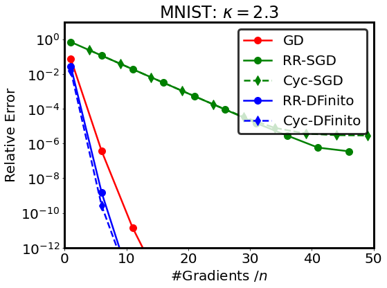
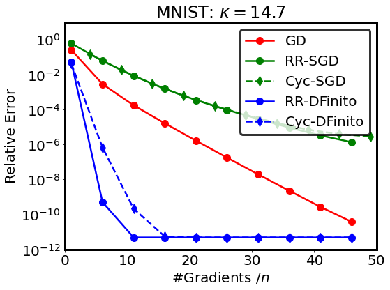
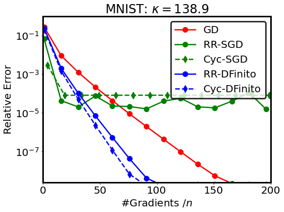
Figure 3: Comparison between DFinito, SGD and GD over MNIST across different conditioning scenarios. The relative error indicates $(\mathbb{E})\|\nabla x-x^{\star}\|^{2}/\|x^{0}-x^{\star}\|^{2}$.

In Fig. 3, it is observed that SGD under without-replacement sampling works, but it will get trapped to a neighborhood around the solution and cannot converge exactly. In contrast, DFinito will converge to the optimum. It is also observed that DFinito can outperform GD in all three scenarios, and the superiority can be significant for certain condition numbers. While this paper establishes that the DFinito under without-replacement sampling shares the same theoretical gradient complexity as GD (see Table 1), the empirical results in Fig. 3 imply that DFinito under without-replacement sampling may be endowed with a better (though unknown) theoretical gradient complexity than GD. We will leave it as a future work.

Influence of various data heterogeneity on optimal cyclic sampling. According to Proposition 5, the performance of DFinito with optimal cyclic sampling is highly influenced by the data heterogeneity. In a highly data-heterogeneous scenario, the ratio $\rho={\mathcal{O}}(1/n)$. In a data-homogeneous scenario, however, it holds that $\rho={\mathcal{O}}(1)$. In this experiment, we examine how DFinito with optimal cyclic sampling converges with varying data heterogeneity. To this end, we construct an example in which the data heterogeneity can be manipulated artificially and quantitatively. Consider a problem in which each $f_{i}(z)=\frac{1}{2}(a_{i}^{T}x)^{2}$ and $r(x)=0$. Moreover, we generate $A=\mbox{col}\{a_{i}^{T}\}\in\mathbb{R}^{n\times d}$ according to the uniform Gaussian distribution. We choose $n=100$ and $d=200$ in the experiment, generate $p_{0}\in\mathbb{R}^{d}$ with each element following distribution ${\mathcal{N}}(0,\sqrt{n})$, and initialize $z_{i}^{0}={p_{0}}/{\sqrt{c}}$, $1\leq i\leq c$ otherwise $z_{i}^{0}=0$. Since $x^{\star}=0$ and $\nabla f_{i}(x^{\star})=0$, we have $z_{i}^{\star}=0$. It then holds that $\|{\boldsymbol{z}}^{0}-{\boldsymbol{z}}^{\star}\|^{2}=\sum_{i=1}^{c}\|z_{i}^{0}\|^{2}=\|p_{0}\|^{2}$ is unchanged across different $c\in[n]$. On the other hand, since $\|{\boldsymbol{z}}^{0}-{\boldsymbol{z}}^{\star}\|^{2}_{\pi^{\star}}=\sum_{i=1}^{c}\frac{i}{n}\frac{\|p_{0}\|^{2}}{c}={\mathcal{O}}(\frac{c}{n}\|p_{0}\|^{2})$, we have $\rho={\mathcal{O}}(c/n)$. Apparently, ratio $\rho$ ranges from ${\mathcal{O}}(1/n)$ to ${\mathcal{O}}(1)$ as $c$ increases from $1$ to $n$. For this reason, we can manipulate the data heterogeneity by simply adjusting $c$. We also depict DFinito with random-reshuffling (8 runs’ average) as a baseline. Figure 4 illustrates that the superiority of optimal cyclic sampling vanishes gradually as the data heterogeneity decreases.

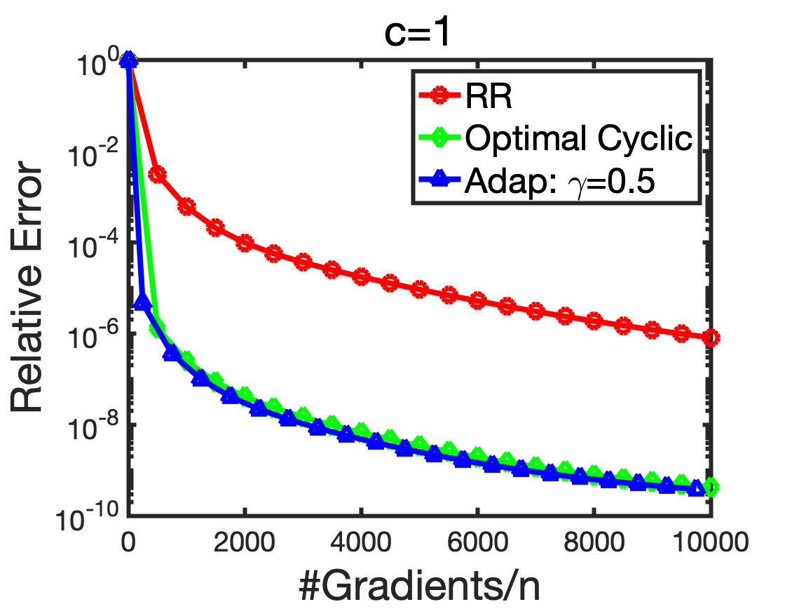
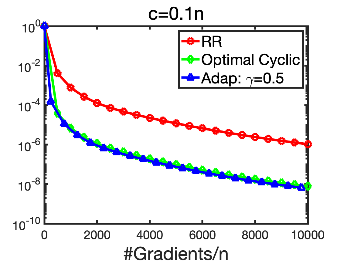
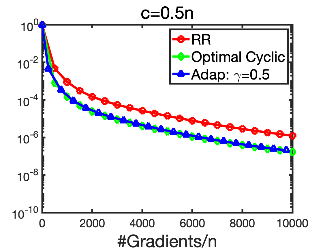
Figure 4: Comparison between various sampling fashions of DFinito across different data-heterogeneous scenarios. The relative error indicates $(\mathbb{E})\|\nabla F(x)\|^{2}/\|\nabla F(x^{0})\|^{2}$.

Comparison with empirically optimal step sizes. Complementary to Sec. 5.1, we also run experiments to compare variance reduction methods under uniform sampling (US) and random reshuffling (RR) with empirically optimal step sizes by grid search, in which full gradient is computed once per two epochs for SVRG. We run experiments for regularized logistic regression task with CIFAR-10 ($\kappa=405$), MNIST ($\kappa=14.7$) and COVTYPE ($\kappa=5.5$), where $\kappa={L}/{\mu}$ is the condition number. All algorithms are averaged through 8 independent runs.

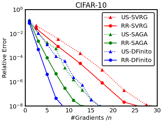
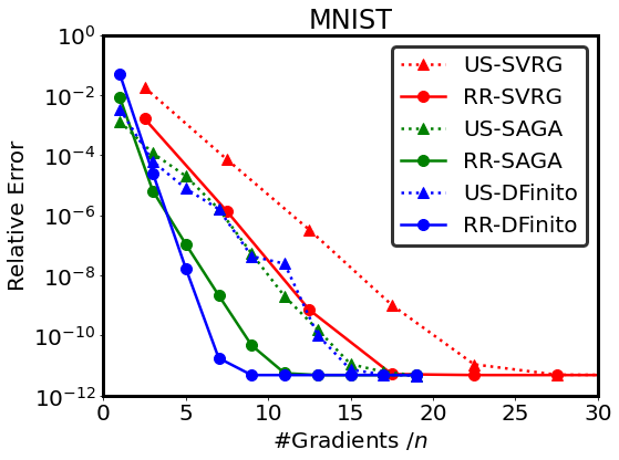
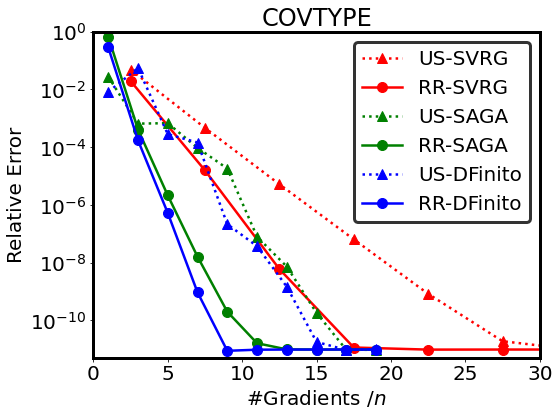
Figure 5: Comparison of variance reduced methods under with/without-replacement sampling. The relative error indicates $(\mathbb{E})\|x-x^{\star}\|^{2}/\|x^{0}-x^{\star}\|^{2}$.

From Figure 5, it is observed that all three variance reduced algorithms achieve better performance under RR, and DFinito outperforms SAGA and SVRG under both random reshuffling and uniform sampling. While this paper and all other existing results listed in Table 1 (including [18]) establish that the variance reduced methods with random reshuffling have worse theoretical gradient complexities than uniform-iid-sampling, the empirical results in Fig. 5 imply that variance reduced methods with random reshuffling may be endowed with a better (though unknown) theoretical gradient complexity than uniform-sampling. We will leave it as a future work.

References

• [1] L. Bottou. Curiously fast convergence of some stochastic gradient descent algorithms. In Proceedings of the symposium on learning and data science, Paris, volume 8, pages 2624–2633, 2009.
• [2] L. Bottou, F. E. Curtis, and J. Nocedal. Optimization methods for large-scale machine learning. Siam Review, 60(2):223–311, 2018.
• [3] S. Boyd, N. Parikh, and E. Chu. Distributed optimization and statistical learning via the alternating direction method of multipliers. Now Publishers Inc, 2011.
• [4] S. S. Chen, D. L. Donoho, and M. A. Saunders. Atomic decomposition by basis pursuit. SIAM review, 43(1):129–159, 2001.
• [5] Y. T. Chow, T. Wu, and W. Yin. Cyclic coordinate-update algorithms for fixed-point problems: Analysis and applications. SIAM Journal on Scientific Computing, 39(4):A1280–A1300, 2017.
• [6] A. Defazio, F. Bach, and S. Lacoste-Julien. SAGA: A fast incremental gradient method with support for non-strongly convex composite objectives. arXiv preprint arXiv:1407.0202, 2014.
• [7] A. Defazio, J. Domke, et al. Finito: A faster, permutable incremental gradient method for big data problems. In International Conference on Machine Learning, pages 1125–1133. PMLR, 2014.
• [8] L. Deng. The mnist database of handwritten digit images for machine learning research. IEEE Signal Processing Magazine, 29(6):141–142, 2012.
• [9] D. L. Donoho. Compressed sensing. IEEE Transactions on information theory, 52(4):1289–1306, 2006.
• [10] M. Gurbuzbalaban, A. Ozdaglar, and P. A. Parrilo. On the convergence rate of incremental aggregated gradient algorithms. SIAM Journal on Optimization, 27(2):1035–1048, 2017.
• [11] M. Gurbuzbalaban, A. Ozdaglar, and P. A. Parrilo. Why random reshuffling beats stochastic gradient descent. Mathematical Programming, pages 1–36, 2019.
• [12] J. Haochen and S. Sra. Random shuffling beats sgd after finite epochs. In International Conference on Machine Learning, pages 2624–2633. PMLR, 2019.
• [13] X. Huang, E. K. Ryu, and W. Yin. Tight coefficients of averaged operators via scaled relative graph. Journal of Mathematical Analysis and Applications, 490(1):124211, 2020.
• [14] R. Johnson and T. Zhang. Accelerating stochastic gradient descent using predictive variance reduction. Advances in neural information processing systems, 26:315–323, 2013.
• [15] A. Krizhevsky. Learning multiple layers of features from tiny images. 2009.
• [16] S. Ma and Y. Zhou. Understanding the impact of model incoherence on convergence of incremental sgd with random reshuffle. In International Conference on Machine Learning, pages 6565–6574. PMLR, 2020.
• [17] J. Mairal. Incremental majorization-minimization optimization with application to large-scale machine learning. SIAM Journal on Optimization, 25(2):829–855, 2015.
• [18] G. Malinovsky, A. Sailanbayev, and P. Richtárik. Random reshuffling with variance reduction: New analysis and better rates. arXiv preprint arXiv:2104.09342, 2021.
• [19] X. Mao, Y. Gu, and W. Yin. Walk proximal gradient: An energy-efficient algorithm for consensus optimization. IEEE Internet of Things Journal, 6(2):2048–2060, 2018.
• [20] G. Mateos, J. A. Bazerque, and G. B. Giannakis. Distributed sparse linear regression. IEEE Transactions on Signal Processing, 58(10):5262–5276, 2010.
• [21] K. Mishchenko, A. Khaled, and P. Richtárik. Proximal and federated random reshuffling. arXiv preprint arXiv:2102.06704, 2021.
• [22] K. Mishchenko, A. Khaled Ragab Bayoumi, and P. Richtárik. Random reshuffling: Simple analysis with vast improvements. Advances in Neural Information Processing Systems, 33, 2020.
• [23] A. Mokhtari, M. Gurbuzbalaban, and A. Ribeiro. Surpassing gradient descent provably: A cyclic incremental method with linear convergence rate. SIAM Journal on Optimization, 28(2):1420–1447, 2018.
• [24] D. Nagaraj, P. Jain, and P. Netrapalli. Sgd without replacement: Sharper rates for general smooth convex functions. In International Conference on Machine Learning, pages 4703–4711. PMLR, 2019.
• [25] Y. Park and E. K. Ryu. Linear convergence of cyclic saga. Optimization Letters, 14(6):1583–1598, 2020.
• [26] X. Qian, A. Sailanbayev, K. Mishchenko, and P. Richtárik. Miso is making a comeback with better proofs and rates. arXiv preprint arXiv:1906.01474, 2019.
• [27] S. Rajput, A. Gupta, and D. Papailiopoulos. Closing the convergence gap of sgd without replacement. In International Conference on Machine Learning, pages 7964–7973. PMLR, 2020.
• [28] H. Robbins and S. Monro. A stochastic approximation method. The annals of mathematical statistics, pages 400–407, 1951.
• [29] R. A. Rossi and N. K. Ahmed. The network data repository with interactive graph analytics and visualization. In AAAI, 2015.
• [30] E. K. Ryu, R. Hannah, and W. Yin. Scaled relative graph: Nonexpansive operators via 2d euclidean geometry. arXiv: Optimization and Control, 2019.
• [31] I. Safran and O. Shamir. How good is sgd with random shuffling? In Conference on Learning Theory, pages 3250–3284. PMLR, 2020.
• [32] M. Schmidt, N. Le Roux, and F. Bach. Minimizing finite sums with the stochastic average gradient. Mathematical Programming, 162(1-2):83–112, 2017.
• [33] T. Sun, Y. Sun, D. Li, and Q. Liao. General proximal incremental aggregated gradient algorithms: Better and novel results under general scheme. Advances in Neural Information Processing Systems, 32:996–1006, 2019.
• [34] R. Tibshirani. Regression shrinkage and selection via the lasso. Journal of the Royal Statistical Society: Series B (Methodological), 58(1):267–288, 1996.
• [35] N. D. Vanli, M. Gürbüzbalaban, and A. Ozdaglar. A stronger convergence result on the proximal incremental aggregated gradient method. arXiv: Optimization and Control, 2016.
• [36] N. D. Vanli, M. Gurbuzbalaban, and A. Ozdaglar. Global convergence rate of proximal incremental aggregated gradient methods. SIAM Journal on Optimization, 28(2):1282–1300, 2018.
• [37] B. Ying, K. Yuan, and A. H. Sayed. Variance-reduced stochastic learning under random reshuffling. IEEE Transactions on Signal Processing, 68:1390–1408, 2020.
• [38] B. Ying, K. Yuan, S. Vlaski, and A. H. Sayed. Stochastic learning under random reshuffling with constant step-sizes. IEEE Transactions on Signal Processing, 67(2):474–489, 2018.
• [39] H.-F. Yu, F.-L. Huang, and C.-J. Lin. Dual coordinate descent methods for logistic regression and maximum entropy models. Machine Learning, 85(1-2):41–75, 2011.
• [40] K. Yuan, B. Ying, S. Vlaski, and A. Sayed. Stochastic gradient descent with finite samples sizes. 2016 IEEE 26th International Workshop on Machine Learning for Signal Processing (MLSP), pages 1–6, 2016.
• [41] P. Zhao and T. Zhang. Stochastic optimization with importance sampling for regularized loss minimization. In international conference on machine learning, pages 1–9. PMLR, 2015.