Critical collapse of a spherically symmetric ultrarelativistic fluid in $2+1$ dimensions

Abstract

We carry out numerical simulations of the gravitational collapse of a perfect fluid with the ultrarelativistic equation of state $P=\kappa\rho$, in spherical symmetry in $2+1$ spacetime dimensions with $\Lambda<0$. At the threshold of prompt collapse, we find type II critical phenomena (apparent horizon mass and maximum curvature scale as powers of distance from the threshold) for $\kappa\gtrsim 0.43$, and type I critical phenomena (lifetime scales as logarithm of distance from the threshold) for $\kappa\lesssim 0.42$. The type I critical solution is static, while the type II critical solution is not self-similar (as in higher dimensions), but contracting quasistatically.

I Introduction

Since the seminal paper of Choptuik [1], it has become clear that for many simple, typically spherically symmetric, self-gravitating systems, such as a scalar field or perfect fluid, the evolutions of generic initial data close to the threshold of black hole formation exhibit several universal properties, which are now collectively called type II critical phenomena at the threshold of gravitational collapse. These are interesting in particular as a route to the formation of naked singularities from regular initial data. (See Ref. [2] for a review).

Consider a one-parameter family of initial data with parameter $p$. Suppose that there exists a threshold value $p=p_{\star}$ so that supercritical initial data, $p>p_{\star}$, eventually collapses into a black hole, while subcritical initial data, $p<p_{\star}$, instead disperses.

In type II critical phenomena, one observes in the case of supercritical data that the black-hole mass obeys a power law $M\propto(p-p_{\star})^{\delta}$, where the exponent $\delta>0$ does not depend on the initial data. (It does depend on the type of matter, within certain universality classes). On the other hand, for subcritical data, it is the maximum curvature that scales, $\text{Ric}_{\text{max}}\propto(p_{\star}-p)^{-2\gamma}$, where $\gamma>0$ is also independent of the initial data.

In $d+1$ dimensions with $d>2$, owing to the fact that mass has dimension length^d-2, the exponents $\delta$ and $\gamma$ are related to each other via $\delta=(d-2)\gamma$, as can be shown from dimensional analysis. These properties near the black-hole threshold are explained through the existence of a critical solution, which has the key properties of being regular, self-similar and having precisely one growing mode. This critical solution appears as an intermediate attractor in the time evolution of any near-critical initial data. As we fine-tune to the black-hole threshold, $p\to p_{\star}$, the (unique) growing mode is increasingly suppressed, so that the critical solution persists on arbitrarily small scales and correspondingly large curvature without collapsing and thus without an event horizon forming. A naked singularity then forms at some finite central proper time for exactly critical data $p=p_{\star}$.

In type I critical phenomena (by contrast to type II), the critical solution is stationary, and instead of mass and curvature scaling, one observes scaling of the lifetime of its appearance as an intermediate attractor, $t_{p}\propto\ln|p-p_{\star}|$.

Critical phenomena in spherical symmetry have been observed in numerous matter models. Since black holes are in general characterized by their mass, charge, and angular momentum, the complete picture of critical phenomena necessarily requires investigation beyond spherical symmetry. However, even generalizing spherically symmetric initial data to axisymmetric ones brings substantial numerical and analytical complications in $3+1$ and higher dimensions. As a result, there have been far fewer studies devoted to studying critical phenomena beyond spherical symmetry.

For this reason, it may be helpful to investigate critical collapse in $2+1$ dimensional spacetime as a toy model. In $2+1$ dimensions, all variables are only functions of time and radius for both spherical symmetry and axisymmetry. This avoids much of the additional technical complication of axisymmetry. As in Ref. [3], we call a solution circularly symmetric if it admits a spacelike Killing vector $\partial_{\theta}$ with closed orbits. More specifically, we call it spherically symmetric if there is no rotation, and we call it axisymmetric with rotation.

An interesting peculiarity of $2+1$ is that black holes cannot form without the presence of a negative cosmological constant. This fact seemingly causes a paradox since, on the one hand, a cosmological constant is required for black holes to form, and thus for the possibility of critical phenomena to occur. On the other hand, one expects any type II critical solution to not depend on the cosmological constant, due to the fact that as the critical solution persists on arbitrarily small length scales, the cosmological constant is expected to become dynamically irrelevant, and so the underlying Einstein and fluid equations become approximately scale invariant. That is probably related at a deep level to the fact that in $2+1$ dimensions the mass is dimensionless and it follows that the usual argument to relate the two exponents $\delta$ and $\gamma$ fails.

Aside from the present paper, the only studies that have investigated critical phenomena in $2+1$ dimensions were restricted to the massless nonrotating [4, 5] and rotating [3] scalar fields. An interesting fact that emerged from those studies is that in $2+1$ dimensions, the nonrotating critical solution for the massless scalar field is continuously self-similar, as opposed to its $3+1$ version, where it is discretely self-similar. Furthermore, the critical solution is well approximated inside the past light cone of its singularity by exactly self-similar solutions to the $\Lambda=0$ Einstein equations. Outside the light cone it can be approximated by a different $\Lambda=0$ exact solution. This patchwork critical solution has three growing modes, but it is conjectured that when $\Lambda$ is taken into account nonperturbatively, the true critical solution is analytic and retains only the top growing mode. This conjecture is in part supported by the fact that under this assumption, one can find a scaling law for the black-hole mass such that $\delta=2\gamma/(2\gamma+1)$, consistent with the numerical results.

In this paper, we study the spherically symmetric collapse of a perfect fluid in $2+1$ in anti-de Sitter (from now, AdS) space with the linear (ultrarelativistic) equation of state $P=\kappa\rho$. Although an important motivation for looking at collapse in $2+1$ dimensions is that axisymmetry with rotation is as simple as spherical symmetry, we begin in this paper with a study of spherically symmetric, nonrotating, collapse.

The structure of the paper is as follows. In Section II, we give a brief description of the equations we solve and their numerical implementation. We refer the reader to Ref. [6] for a complete discussion and details of our numerical implementation. In Sec. III, we present the results of our numerical investigation of the threshold of prompt collapse for a spherically symmetric perfect fluid in $2+1$ dimensions. We show evidence of both type I and type II behavior depending on the value of $\kappa$. The type I critical solution is static, describing a metastable star. The type II critical solution shrinks quasistatically, moving adiabatically through the family of static stars. (A slightly different approximation is needed in the thin atmosphere of the star, where the outflow speed is relativistic.) Sec. IV contains our conclusions. In appendixes, we show that no regular continuously self-similar solution exists, review the static solutions, and show how they relate to the quasistatic solution.

II Einstein and Fluid equations in polar-radial coordinates

We refer the reader to the companion paper [6] for a complete discussion. We use units where $c=G=1$.

In spherical symmetry in $2+1$ dimensions, we introduce generalised polar-radial coordinates as

$$ds^{2} = -\alpha^{2}(t,r)\,dt^{2}+a^{2}(t,r)R^{\prime 2}(r)\,dr^{2}$$ (1)

$$+R^{2}(r)d\theta^{2}.$$

Note that our choice $g_{rr}=a^{2}R^{\prime 2}$ makes $a$ invariant under a redefinition of the radial coordinate, $r\to\tilde{r}(r)$.

We impose the gauge condition $\alpha(t,0)=1$ ($t$ is proper time at the center), and the regularity condition $a(t,0)=1$ (no conical singularity at the center). The gauge is fully specified only after specifying the function $R(r)$. In our numerical simulations we use the compactified coordinate

$$R(r)=\ell\tan(r/\ell),$$ (2)

with different values of the cosmological scale $\ell$ defined by

$$\ell:={1\over\sqrt{-\Lambda}},$$ (3)

but for clarity we write $R$ and $R^{\prime}$ rather than the explicit expressions.

In our coordinates, the Misner-Sharp mass $M$ is given by

$$M(t,r) := {R^{2}\over\ell^{2}}-{1\over a^{2}}.$$ (4)

The stress-energy tensor for a perfect fluid is

$$T_{ab}=(\rho+P)u_{a}u_{b}+Pg_{ab},$$ (5)

where $u^{a}$ is tangential to the fluid worldlines, with $u^{a}u_{a}=-1$, and $P$ and $\rho$ are the pressure and total energy density measured in the fluid frame. In the following, we assume the one-parameter family of ultrarelativistic fluid equations of state $P=\kappa\rho$, where $0<\kappa<1$.

The 3-velocity is decomposed as

$$u^{\mu}=\{u^{t},u^{r},u^{\theta}\}=\Gamma\left\{\frac{1}{\alpha},\frac{v}{aR^{\prime}},0\right\},$$ (6)

where $v$ is the physical velocity of the fluid relative to observers at constant $R$, with $-1<v<1$, and

$$\Gamma:=\left(1-v^{2}\right)^{-1/2}$$ (7)

is the corresponding Lorentz factor.

The stress-energy conservation law $\nabla_{a}T^{ab}=0$, which together with the equation of state governs the fluid evolution, can be written in balance law form

$${\bf q}_{,t}+{\bf f}_{,r}={\bf S},$$ (8)

where we have defined the conserved quantities

$${\bf q}:=\{\Omega,Y\}$$ (9)

given by

$$\Omega := R^{\prime}R\tau,$$ (10)

$$Y := R^{\prime}v\sigma,$$ (11)

the corresponding fluxes ${\bf f}$ given by

$$f_{(\Omega)} := {\alpha\over a}Rv\sigma,$$ (12)

$$f_{(Y)} := {\alpha\over a}(P+v^{2}\sigma),$$ (13)

the corresponding sources ${\bf S}$ given by

$$S_{(\Omega)} := 0,$$ (14)

$$S_{(Y)} := a\alpha RR^{\prime}\Bigl{[}-\frac{v^{2}\sigma}{a^{2}R^{2}}+2P(8\pi P-\Lambda)$$ (15)

$$-\sigma\left(1-v^{2}\right)(16\pi P-\Lambda)\Bigr{]},$$

and the shorthands

$$\sigma := \Gamma^{2}(1+\kappa)\rho,$$ (16)

$$P := \kappa\rho,$$ (17)

$$\tau := \sigma-P.$$ (18)

In Eq. (15), we have already used some of the Einstein equations to express metric derivatives in terms of stress-energy terms.

At any given time, the balance laws [Eq. (8)] are used to compute time derivatives of the conserved quantities $\bf q$, using standard high-resolution shock-capturing methods. The ${\bf q}$’s are evolved to the next time step via a second-order Runge-Kutta step. At each (sub-)time step, the metric variables are then updated through the Einstein equations

$$(\ln\alpha a)_{,r} = 8\pi a^{2}RR^{\prime}(1+v^{2})\sigma,$$ (19)

$$M_{,r} = 16\pi\Omega.$$ (20)

Our numerical scheme is totally constrained, in the sense that only the matter is updated through evolution equations. Our numerical scheme exploits this to make $\Omega$ and $M$ exactly conserved in the discretized equations.

Another useful Einstein equation, compatible with the above ones via stress-energy conservation, is

$$M_{,t}=-16\pi f_{(\Omega)}.$$ (21)

III Numerical results

III.1 Initial data

The numerical grid is equally spaced in the compactified coordinate $r$, as defined in Eq. (2), with $800$ grid points, and for all values of $\Lambda$ its outer boundary is fixed at the same area radius $R$. For reasons that will be made clear, we fix, unless otherwise stated, $R_{\text{max}}\simeq 1.25$ for $\kappa\geq 0.43$ and $R_{\text{max}}\simeq 10$ for $\kappa\leq 0.42$.

We choose to initialize the intermediate fluid variables

$$\omega:={\Omega\over R^{\prime}R},\qquad\eta:={Y\over R^{\prime}R}$$ (22)

as double Gaussians in $R$,

$$\omega(0,R) =\frac{p_{\omega}}{2}\left(e^{-\left(\frac{R-R_{\omega}}{\sigma_{\omega}}\right)^{2}}+e^{-\left(\frac{R+R_{\omega}}{\sigma_{\omega}}\right)^{2}}\right),$$ (23)

$$\eta(0,R) =\frac{p_{\eta}}{2}\left(e^{-\left(\frac{R-R_{\eta}}{\sigma_{\eta}}\right)^{2}}+e^{-\left(\frac{R+R_{\eta}}{\sigma_{\eta}}\right)^{2}}\right).$$ (24)

where $p_{\omega}$ and $p_{\eta}$ are the magnitudes, $R_{\omega}$ and $R_{\eta}$ are the displacements from the center, and $\sigma_{\omega}$ and $\sigma_{\eta}$ are the widths of the Gaussians. Note that $p_{\omega}$ has dimension length^-2, while $p_{\eta}$ is dimensionless.

For $\kappa\geq 0.43$, we fix $\sigma_{\omega}=0.2$ and $\sigma_{\eta}=0.15$ and consider three types of initial data:

1) Time-symmetric off-centered: $p_{\eta}=0$, $R_{\omega}=0.4$,

2) Time-symmetric centered: $p_{\eta}=0$, $R_{\omega}=0$, and

3) Initially ingoing off-centered: $p_{\eta}=-0.2$, $R_{\omega}=R_{\eta}=0.4$.

For $\kappa\leq 0.42$, we consider time-symmetric off-centered and ingoing initial data as given above, and time-symmetric centered $R_{\omega}=0$, $\sigma_{\omega}=0.05$, $p_{\eta}=0$, and $\sigma_{\eta}=0.15$.

In all cases, the remaining parameter $p_{\omega}=:p$ is fine-tuned to the black-hole threshold.

The space of initial data parametrized by $p$ can be subdivided into four regions with boundaries $p_{-}<p_{\star}<p_{+}$ as follows: At $p=p_{-}$, the total mass is zero, $M_{\infty}=0$, while $p=p_{\star}$ corresponds to the critical value separating subcritical (initially dispersing) from supercritical (promptly collapsing) initial data. Finally, $p_{+}$ is defined so that a trapped surface, characterized by $(\nabla R)^{2}=0$, is already present for initial data with $p>p_{+}$.

Initial data ($\kappa=0.5$)	$p_{-}$	$p_{\star}$	$p_{+}$
Off-centered, $\tilde{\mu}=0.01$,	0.280	0.309	0.324
Off-centered, $\tilde{\mu}=0.1$,	0.280	0.402	0.612
Centered, $\tilde{\mu}=0.1$,	0.995	1.174	1.354
Ingoing, $\tilde{\mu}=0.1$,	0.280	0.377	0.612
Off-centered, $\tilde{\mu}=1$,	0.280	0.531	3.087
Off-centered, $\tilde{\mu}=10$,	0.280	0.572	27.33

Table 1: The relation between $p_{-}$, $p_{\star}$, $p_{+}$, and the initial data that we are considering in this paper for $\kappa=0.5$.

In $2+1$, black-hole solutions with $M_{\infty}>0$ are separated from the vacuum AdS solution $M_{\infty}=-1$ by a mass gap [7], so that no initial data with $p<p_{-}$ can collapse into a black hole.

As already stated, in $2+1$ dimensions, a negative cosmological constant is necessary for the formation of black holes, and thus for critical phenomena to occur. Since the cosmological constant introduces a length scale $\ell$ into the system, we need to consider different sizes of the initial data with respect to $\ell$, which can be quantified by considering the dimensionless quantity

$$\tilde{\mu}:=-\Lambda\sigma_{\omega}^{2}=\left(\frac{\sigma_{\omega}}{\ell}\right)^{2}.$$ (25)

$\sigma_{\omega}$ is kept fixed as given before, while we vary $\tilde{\mu}$ and thus $\ell$. For $\kappa\geq 0.43$, we set $\tilde{\mu}=0.1$. For $\kappa=0.5$, we in addition study the cases $\tilde{\mu}=0.01$, $1$ and $10$, corresponding to a range of values of the cosmological length scale that are “small” to “large” compared to the initial data. For $\kappa\leq 0.42$, we set $\Lambda=-\pi^{2}/4$ ($\tilde{\mu}\simeq 0.006$).

In Table 1, we record the values of $p_{-}$, $p_{\star}$ and $p_{+}$ for different families of initial data with $\kappa=0.5$. Note that, unlike in higher dimensions, $p_{-}\to p_{+}$ as $\Lambda\to 0$.

Regularity at the timelike outer boundary of spacetimes with $\Lambda<0$ does not allow a stress-energy flux through it. For a scalar field, this enforces homogeneous Dirichlet (reflecting) boundary conditions, whereas for perfect fluid matter its energy density needs to vanish at the boundary. Dynamically, this is enforced by an inward Hubble acceleration of the matter, so that any test particles on timelike geodesics, at least, must turn around inwards. Hence, it is a priori possible for data to collapse only after being reflected, possibly several times, from the boundary, as was observed for the massless scalar field in Ref. [8].

As we impose (unphysical) outer boundary conditions at a finite radius, most of the energy that is outgoing in fact leaves the numerical domain. Thus, we cannot directly investigate the reflective property of AdS here. In this sense, we fine-tune to the threshold of prompt collapse.

Independently, because of our polar time slices, our code stops when a trapped surface first appears on a time slice, and so we cannot obtain the final black-hole mass, so in this sense we measure the mass of the apparent horizon when it first touches a polar time slice. (However, it is likely that given enough time, all matter eventually falls into the black hole, so the black-hole mass becomes equal to the total mass $M_{\infty}$.)

In the following, we are interested in initial data where $p\simeq p_{\star}$ and we refer to “sub$n$” data as subcritical data for which $\log_{10}(p_{\star}-p)\simeq-n$, and to “super$n$” as supercritical data with $\log_{10}(p-p_{\star})\simeq-n$.

III.2 Overview of results

For the equation of state $P=\kappa\rho$ with $\kappa\lesssim 0.42$, we find type I critical phenomena: time evolutions of initial data near the black-hole threshold approach a static solution before either collapsing to a black hole or dispersing, and the time this intermediate attractor is seen for scales as $t_{p}\sim-\ln|p-p_{\star}|$. The static type I critical solution is not universal.

For $\kappa\gtrsim 0.43$ we observe scaling of the apparent horizon mass and maximum curvature as powers of distance to the threshold of (prompt) collapse, characteristic of type II critical phenomena. The type II critical solution is universal but not self-similar. It is instead quasistatic, running adiabatically through the one-parameter family of regular static solutions.

III.3 $\kappa\lesssim 0.42$: Type I critical collapse

III.3.1 Lifetime scaling

In type I critical phenomena, the critical solution is stationary or time-periodic instead of self-similar. Furthermore, there is a nonvanishing mass gap at the black-hole threshold, and so the critical solution is usually thought of as a metastable star.

In Fig. 1, we plot the apparent horizon mass $M_{\text{AH}}$ against $p-p_{\star}$ for different values of $\kappa$. For $\kappa\leq 0.42$, we find the existence of a mass gap, corresponding to type I critical phenomena. Similarly, the maximum curvature is bounded above, but we choose not to show it here in order to avoid cluttering. This plot was obtained using a second-order limiter. With a first-order (Godunov) flux limiter, the mass scales, but it does so in a step-size manner. We believe that this is an artifact of the Godunov limiter.

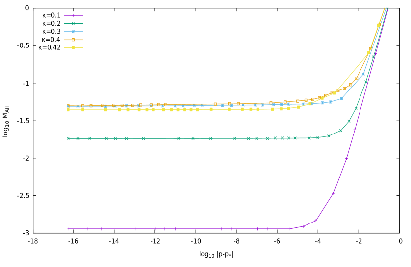
Figure 1: Apparent horizon mass for different values of $\kappa\leq 0.42$. The mass does not scale, and there is a mass gap at the black-hole threshold instead. We similarly find an upper bound for the maximum curvature.

To further investigate the type I behavior, we need to define a measure of the length scale of the solution. We can do this by recording, for example, the central density and mass at the outer boundary, defined by

$$\rho_{0}(t):=\rho(t,0),\quad M_{\text{OB}}(t):=M(t,R_{\text{max}})$$ (26)

and the radius where the mass vanishes,

$$M(t,R_{M}(t)):=0.$$ (27)

In Fig. 2, we plot $\sqrt{\rho_{0}^{-1}}$, $\sqrt{M_{\text{OB}}}$, and $R_{M}$ for off-centered (left) and centered (right) initial data with $\kappa=0.4$, evolved with the monotonized central (MC) and Godunov limiters, respectively. Both sets of results are shown at different levels of fine-tuning.

In both cases, we see that $R_{M}$ and $M_{\text{OB}}$ are approximately constant during the critical regime. In the former case, the central density is subject to the apparition of periodic shocks, which cause the periodic structure for $R_{M}$ and $\rho_{0}$. In the latter case, the periodic shocks are not present and the density converges to some finite value. We find that in this case $M_{\text{OB}}$ and $R_{M}$ evolve slightly. This is due to the fact that the Godunov limiter is known to introduce a great deal of numerical diffusion [9]. A benefit of this diffusion is that the aforementioned shocks, developing at the outer boundary, are not present, and the density converges to some finite value. In both cases, however, less fine-tuned initial data peel off from the critical behavior faster than more fine-tuned data. This suggests that the critical solution has a single growing mode which is being progressively suppressed as we fine-tune to the black-hole threshold.

The shocks mentioned above in the case of the second-order limiter originate from the unphysical boundary conditions imposed at the numerical outer boundary. Although one might wonder how these shocks interact with the behavior of the critical solution, one can still reasonably believe that the type I phenomena are not a numerical artifact. One reason is that we still find type I phenomena in the second set of simulations described above, where the aforementioned instabilities do not occur.

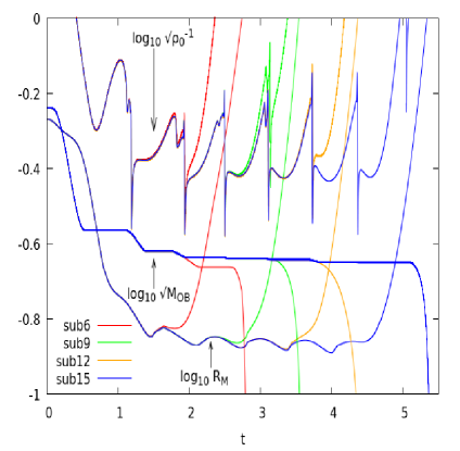
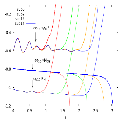
Figure 2: Linear-log-plot of $R_{M}(t)$, $\sqrt{\rho_{0}^{-1}(t)}$, and $\sqrt{M_{\text{OB}}(t)}$ for the evolution of sub6-sub15 initial data with $\kappa=0.4$. The plot on the left shows off-centered initial data, evolved with the MC limiter. The plot on the right shows more compact and centered initial data, evolved with the Godunov limiter.

As the critical solution does not depend on $t$, for its linear perturbations we can make the ansatz

$$\delta Z(t,x)=\sum_{i=0}^{\infty}C_{i}(p)\,e^{\sigma_{i}{t\over\ell}}\,Z_{i}(x),$$ (28)

where $Z$ stands for any dimensionless metric or matter variable.

By definition, the critical solution has a single growing mode, ${\rm Re}\,\sigma_{0}>0$. Since the solution is exactly critical at $p=p_{\star}$, this implies that $C_{0}(p)\sim p-p_{\star}$.

We define the time $t=t_{p}$ to be the time where the growing perturbation becomes nonlinear. We can take this to be

$$(p-p_{\star})e^{\sigma_{0}{t_{p}\over\ell}}\simeq 1,$$ (29)

and so

$$t_{p}=\frac{\ell}{\sigma_{0}}\ln|p-p_{\star}|+\text{constant}.$$ (30)

The exponent $\sigma_{0}$ for $\kappa=0.4$, for example, can be read off from Fig. 2. Specifically, we treat the value of $p$ of our best fine-tuned data as a proxy for $p_{\star}$. We then record, as a function of $p-p_{\star}$ from sub8 to sub15 initial data, the time $t=t_{p}$ where, say $R_{M}$, peels off. We similarly compute $\sigma_{0}$ for other values of $\kappa$.

In Table 2, we show $\sigma_{0}$ for different values of $\kappa$ and find that $\sigma_{0}$ increases approximately linearly with $\kappa$.

$\kappa$	$\sigma_{0}$
$0.30$	4.97
$0.32$	5.54
$0.34$	5.89
$0.36$	6.46
$0.38$	7.19
$0.40$	8.84
$0.42$	9.70

Table 2: The value of $\sigma_{0}$ as a function of $\kappa$. We have obtained $\sigma_{0}$ from the lifetime scaling [Eq. (30)] of the critical solution.

III.3.2 The critical solution

All spherically symmetric static solutions (and in fact all rigidly rotating axisymmetric stationary solutions) with $\Lambda\leq 0$ were found in Ref. [10], for arbitrary fluid equations of state.

In Ref. [11], we highlighted the existence of a two-parameter family of rigidly rotating static star solutions, for any causal equation of state, which are analytic everywhere including at the center, and have finite total mass $M$ and angular momentum $J$. In particular, there is a one-parameter family of static solutions with a regular center and finite total mass, parameterised by an overall length scale $s$, see Appendix B for a summary of the notation and results for the specific equation of state $P=\kappa\rho$.

The equation of state $P=\kappa\rho$ itself is scale invariant, so in the absence of a cosmological constant, the dimensionless quantities

$$Z:=\{R^{2}\rho,M,\alpha\}$$ (31)

characterizing a static solution can then only depend on $R/s$. However, the cosmological constant breaks scale invariance and so the family of static solutions instead takes the form

$$Z=\check{Z}\left({R\over s},-\Lambda s^{2}\right),$$ (32)

where $\check{Z}$ is the corresponding exact static solution.

In what follows, all the quantities referring to the static solution have a check symbol, as in Eq. (32).

For $\Lambda<0$, these stars have finite total mass (and to be a critical solution, the total mass needs to be positive), but the density $\rho$ vanishes only asymptotically at infinity. For small $\mu:=-\Lambda s^{2}$, the star has an approximate surface [Eq. (76)] at $R\simeq s\check{x}_{c}$, separating the star proper from a thin atmosphere with negligible self-gravity. (We note that in the singular limit $\Lambda=0$, the atmosphere disappears completely. The exterior solution is now vacuum with $M=0$, and in particular the spatial geometry is a cylinder of constant radius.)

In Fig. 3, we provide some evidence that the critical solution is related to this family of static solution by plotting our best subcritical solution (with the Godunov limiter) at time $t\simeq 2$. This is compared to a member of the static solution, selected to satisfy the condition

$$\Lambda=8\pi\kappa\rho_{0}(t)-\frac{1}{s^{2}(t)}.$$ (33)

at that time. This ensures that the central density is the same in the numerical and exact static solutions. We find reasonable agreement between the numerical and exact static solutions out to the surface and slightly beyond.

This can also be seen as a further consistency check that the type I phenomena are not a numerical artifact as it is otherwise unlikely that the numerical solution approaches an exact solution to the Einstein equations.

We find that the critical solution has different masses for the off-centered, centered and ingoing families of initial data, so clearly the type I critical solution is not universal.

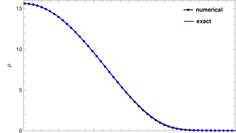
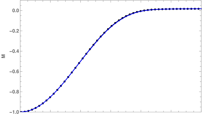
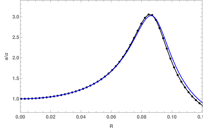
Figure 3: Plots of $M$, $\rho$, and $a/\alpha$ for sub14 centered initial data evolved with the Godunov limiter (black) with $\kappa=0.4$ at $t\simeq 2$. This is compared with the exact static solution (blue), matched using Eq. (33).

III.4 $\kappa\gtrsim 0.43$: Type II critical collapse

III.4.1 Curvature and mass scaling

In type II critical collapse, in a region near the center, curvature becomes arbitrarily large as the solution approaches a critical solution with the following defining properties: it is regular, universal with respect to the initial data, shrinking, and it has precisely one unstable mode.

In spherical symmetry, and assuming a continuous, rather than discrete, scaling symmetry, there exists some adapted coordinate $x=R/s(t)$, for some function $s(t)$, where $t$ is central proper time such that a vector $Z(t,x)$ of suitably scaled variables that characterizes a circularly symmetric solution of the Einstein and matter equations, is only a function of $x$, $Z(t,x)=Z_{\star}(x)$.

Since the existence of such a solution is a consequence of the (approximate) scale invariance of the underlying Einstein and matter equations, one would expect any quantity of dimension lengthⁿ to scale as $s(t)^{n}$. In particular, in $d+1$ spacetime dimensions, one would expect the maximum curvature (and apparent horizon mass) to scale as

$$\text{Ric}_{\text{max}}\sim s(t_{\#})^{-2},\quad M_{\text{AH}}\sim s(t_{\#})^{d-2}$$ (34)

where $s(t_{\#})$ is the smallest scale the solution reaches before either dispersing or forming an apparent horizon.

As the critical solution is independent of $t$, for its linear perturbations we can make the ansatz

$$\delta Z(t,x)=\sum_{i=0}^{\infty}C_{i}(p)\,s(t)^{-\lambda_{i}}\,Z_{i}(x).$$ (35)

We define $t=t_{\star}$ to be the time where $s(t_{\star})=0$. Since by definition the critical solution has a single growing mode, ${\rm Re}\,\lambda_{0}>0$, near the critical time $t\lesssim t_{\star}$, all other (decaying, ${\rm Re}\,\lambda_{i}<0$) modes are negligible, and we therefore need the fact that $C_{0}(p)\sim p-p_{\star}$.

The time $t=t_{\#}$ when the growing perturbation becomes nonlinear occurs when $(p-p_{\star})s(t_{\#})^{-\lambda_{0}}\sim\mathcal{O}(1)$. Together with Eq. (34), one then deduces $\rho_{\text{max}}$ and $M_{\text{AH}}$ scale according to the power laws

$$M_{\text{AH}} =c_{M}|p-p_{\star}|^{\delta},$$ (36)

$$\text{Ric}_{\text{max}}\sim\rho_{\text{max}} =-\Lambda c_{\rho}|p_{\star}-p|^{-2\gamma},$$ (37)

where $c_{M}$ and $c_{\rho}$ are dimensionless constants, $\gamma=1/\lambda_{0}$, and in space dimension $d\geq 3$, $\delta=(d-2)\gamma$.

We have here slightly generalized the discussion in Ref. [2], where $s(t)\propto t_{\star}-t$, with $t$ as the proper time at the origin, because the critical solution is continuously self-similar (homothetic). We will see that the critical solution for type II critical fluid collapse in 2+1 dimensions is not self-similar, but the generalized discussion still applies.

In $d=2$, the mass scaling and the value of $\delta$ cannot be derived by the simple dimensional analysis outlined above. In Ref. [4], Pretorius and Choptuik proposed that from the expression (4) for the Misner-Sharp mass, one has $M_{\text{AH}}=-\Lambda R_{\text{AH}}^{2}$, and so one would expect $M_{\text{AH}}\sim s(t_{\#})^{2}$. Furthermore, from the dimension of the curvature, one also expects $\rho_{\text{max}}^{-1}\sim s(t_{\#})^{2}$, which, combined with the previous expression, implies

$$M_{\text{AH}}\sim-\Lambda\rho_{\text{max}}^{-1},$$ (38)

or $\delta=2\gamma$. Although we will see that such a relation holds in the present case, the explanation should explicitly depend on the matter field under consideration, since a different relation has been shown to hold for the massless scalar field [5], where it was shown that $R_{\text{AH}}$ does not scale as suggested by its dimension.

In our numerical investigation of type II critical collapse, we focus on the equation of state with $\kappa=0.5$, where we have investigated possible critical behavior by bisecting between subcritical and supercritical data. Due to the small values of $\delta$ and $\gamma$ (as compared to critical fluid collapse in 3+1 dimensions [12]), we observe scaling all the way down to $\log_{10}|p-p_{\star}|\simeq-15$ in double precision, even at fairly low numerical resolution and without mesh refinement, as the range of length scales is not large. We make use of this, or compensate for it, by working in quadruple precision, even at fairly low grid resolution. We can then fine-tune to about $\log_{10}|p-p_{\star}|\simeq-25$ before we lose resolution (without mesh refinement).

We observe that for $\tilde{\mu}=0.01$, $0.1$, $1$, and $10$, as we fine-tune to the black-hole threshold, $M_{\text{AH}}$ becomes arbitrarily small while $\rho_{\text{max}}$ becomes arbitrarily large. Moreover, both quantities scale so that their product is constant,

$$\frac{\rho_{\text{max}}M_{\text{AH}}}{-\Lambda}\simeq\mathcal{C},$$ (39)

where $\mathcal{C}$ is a dimensionless constant independent of $\Lambda$.

Furthermore, we empirically observe that for sub15 data onwards, $M_{\text{AH}}$ and $\rho_{\text{max}}$ are well fitted by power laws (36) and (37), respectively, where the exponents are related by

$$\delta\simeq 2\gamma.$$ (40)

Note that from Eq. (39), $c_{\rho}c_{M}=\mathcal{C}$. The scaling laws are illustrated in Fig. 4, which shows $\ln M_{\text{AH}}$ and $-\ln\rho_{\text{max}}$ against $\ln|p-p_{\star}|$.

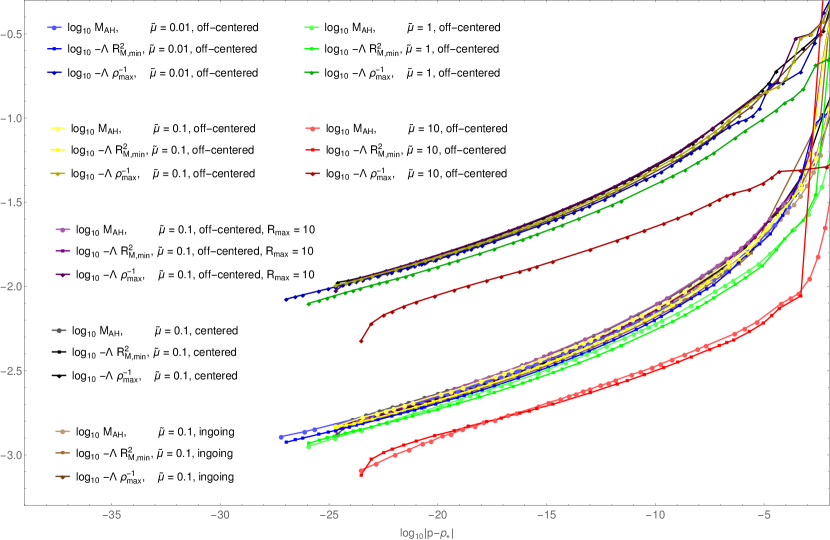
Figure 4: Log-log plot demonstrating the power-law scaling of $\rho_{\text{max}}$ (upper group of curves), $M_{\text{AH}}$ and $R_{M\text{,min}}$ (lower group of curves) for different values of the cosmological constant, different outer boundary locations, and different initial data. The plot gives evidence that the relations $-\Lambda\rho_{\text{max}}^{-1}\sim M_{\text{AH}}\simeq-\Lambda R^{2}_{M\text{,min}}$ hold, are universal, and are independent of the cosmological constant. The constants $c_{M}$, $c_{\rho}$, and $c_{R}$ in general depend on the family of initial data and $\tilde{\mu}$, but here are almost universal except for $\tilde{\mu}=10$ (curves somewhat below each group).

In Table 3, we record the values of $\mathcal{C}$, $\delta$, and $2\gamma$ for different initial data and $\tilde{\mu}$. We find that the relation in Eq. (39) holds independently of the initial data. On the other hand, we cannot exclude that the exponents $\delta$ and $2\gamma$ depend weakly on $\tilde{\mu}$. Similarly, we find that $\mathcal{C}$ may weakly depend on both the initial data and $\tilde{\mu}$.

We have checked that our results are not affected by the location of the (unphysical) outer boundary $R=R_{\rm max}$ by performing a bisection with $R_{\text{max}}\simeq 10$.

Initial data ($\kappa=0.5$)	$\mathcal{C}$	$\delta$	$2\gamma$
Off-centered, $\tilde{\mu}=0.01$	0.148	0.0364	0.0371
Off-centered, $\tilde{\mu}=0.1$	0.151	0.0413	0.0409
Centered, $\tilde{\mu}=0.1$	0.170	0.0440	0.0410
Ingoing, $\tilde{\mu}=0.1$	0.156	0.0417	0.0409
Off-centered, $\tilde{\mu}=1$	0.161	0.0410	0.0389
Off-centered, $\tilde{\mu}=10$	0.167	0.0427	0.0391

Table 3: The values of $\mathcal{C}$, $\delta$, and $2\gamma$ for different initial data and $\tilde{\mu}$, all for $\kappa=0.5$. These values are obtained by fitting a straight line to the log-log plots from super/sub15 to super/sub25 data points. (We only go to super/sub22 for $\tilde{\mu}=10$).

III.4.2 The critical solution

In $3+1$ dimensions or higher, the critical solution exhibiting type II phenomena has always been found to be either continuously or discretely self-similar, depending on the matter field under consideration. The critical solution then only depends on $x=R/(t_{\star}-t)$ (in polar-radial coordinates, with $t$ normalized to be proper time at the center) in the continuous case, while in the discrete case, it also depends on the logarithm of $t_{\star}-t$, with some period $\Delta$.

In $2+1$ dimensions, the presence of a cosmological constant is required for black holes to exist and thus for the possibility of critical phenomena to occur. Therefore, the Einstein equations are not scale-free, and as a consequence the critical solution cannot be exactly continuously or discretely self-similar. However, as the solution contracts to increasingly smaller scales, one expects the effect of the cosmological constant to become dynamically irrelevant. The critical solution could then again be approximated by an expansion in powers of (length scale of the solution)/$\ell$, where the zeroth-order term is a self-similar solution of the $\Lambda=0$ Einstein and matter equations. This is actually the case for the massless scalar field [5], where the critical solution is well approximated near the center by a continuously self-similar solution of the $\Lambda=0$ field equations, but where the presence of $\Lambda$ becomes relevant near the light cone.

However, it is shown in Appendix A that a regular self-similar solution does not exist for the perfect fluid with a barotropic equation of state in $2+1$ (in contrast to higher dimensions, where it is the type II critical solution). Given that we have type II critical collapse nevertheless, this raises the question of what form $s(t)$ takes.

In order to quantify $s(t)$, one can consider “candidate” functions $R_{M}(t)$ [defined previously; see Eq. (27)] and $R_{v}(t)$, defined by

$$v(t,R_{v}(t)):=0.$$ (41)

Both of these functions are expected to be related to the size of the solution $s(t)$. We characterize the minimum size of the solution by $R_{M\text{,min}}:=\min\limits_{t}R_{M}(t)$. It turns out that this also scales as suggested by its dimension, i.e.,

$$R_{\text{M,min}}=\ell c_{R}|p-p_{\star}|^{\gamma},$$ (42)

where $c_{R}$ is a dimensionless constant; see Fig. 4.

In $2+1$ dimensions, the total mass of the spacetime must be positive for black holes to form. It is therefore instructive to see the evolution of the mass in the case of near-critical data. In Fig. 5, we plot $M(t_{i},R)$ (left panel) and $v(t_{i},R)$ (right panel) for sub25 off-centered initial data at times $t_{i}=0$, $0.25$, $0.5$, $\cdots$, $2.25$, $2.37$, $2.5$. Near the initial time, one part of the initial data shrinks, while the other part leaves the numerical domain, causing the mass at the numerical outer boundary to quickly decrease (green). As the data approaches a critical regime (red), the mass profile shrinks with $t$ for $R\leq R_{M}(t)$, while for $R\geq R_{v}(t)$, the mass is approximately constant in $R$ but asymptotes to $0^{+}$ exponentially in $t$ (see inset). The in-between region, $R_{M}(t)<R<R_{v}(t)$, is a transition region whose width shrinks with $t$; see Fig. 6. For our best subcritical data, we find $t_{\#}\simeq 2.1$, after which the mass disperses (blue) and the velocity is a positive function of $R$ and attains values close to $1$ (the speed of light).

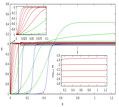
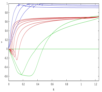
Figure 5: Plots of $M(t_{i},R)$ (left) and $v(t_{i},R)$ (right) at different times $t_{i}\simeq 0.$, $0.25$, $0.5$, $\cdots$, $2.25$, $2.37$, $2.5$ for our best subcritical data. The density profile shrinks and a large part of the total mass leaves the numerical domain (green). The evolution enters a critical regime (red) before dispersing (blue). In the bottom inset, the logarithm of the mass at large radius is plotted during the critical regime to show that it is almost constant in space and decays exponentially to zero. In the top inset, note that the contraction slows down. During dispersion, the velocity is close to $1$ at $R\simeq 0.2$, causing numerical errors.

From dimensional analysis, the quantities $R_{M}(t)$ and $R_{v}(t)$, as well as the central proper density $\rho_{0}(t)$, are expected to be related to $s(t)$ as

$$\rho_{0}\sim s(t)^{-2},\qquad R_{M}(t)\sim R_{v}(t)\sim s(t).$$ (43)

In Fig. 6, we plot the logarithms of $R_{M}(t)$, $R_{v}(t)$, $\sqrt{\rho_{0}^{-1}(t)}$, and $\sqrt{M_{\text{OB}}(t)}$ for sub5, sub10, sub15, sub20 and sub25 data. We find that these quantities are exponential functions of $t$, thus suggesting that $s(t)$ should also be an exponential. It should be noted here that for our best subcritical data, the duration of the critical regime, $\Delta t\simeq 1$, is sufficiently long to distinguish an exponential from a power law.

The exponential scaling lasts longer the more fine-tuned the initial data is to the black-hole threshold, while less fine-tuned initial data peel off sooner. This indicates that the critical solution has a single growing mode that is being increasingly suppressed as we fine-tune to the black-hole threshold.

It is useful to compare this plot with the left plot of Fig. 2, which was obtained with the same initial data and limiter but with $\kappa=0.4$. There the proxies for $s(t)$ were approximately constant, while here we see clear exponential shrinking. Note that we do not observe here any numerical instability originating from the numerical outer boundary, as we did for $\kappa\leq 0.42$. The reason for this is that for $\kappa=0.5$, near the numerical outer boundary, all three characteristic speeds of the fluid are positive.

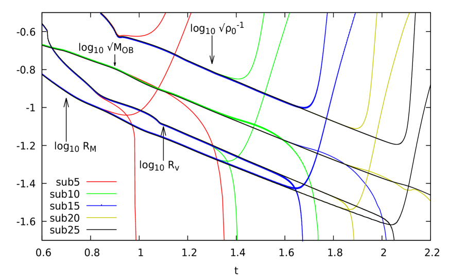
Figure 6: Log plot of $R_{M}(t)$, $R_{v}(t)$, $\sqrt{\rho_{0}^{-1}(t)}$, and $\sqrt{M_{\text{OB}}(t)}$, for sub5 to sub25 off-centered initial data. We observe that as we fine-tune to the black-hole threshold, the solution approaches an intermediate attractor solution in which $R_{M}$, $R_{v}$, $\rho_{0}^{-1}$, and $M_{\text{OB}}$ decrease exponentially. Less fine-tuned initial data peel off from this critical line sooner than more fine-tuned data, leading to critical scaling of the maximum density, etc.

A striking feature implied by the fact that $s(t)$ is exponential instead of polynomial in $t$ is that $t_{\star}=\infty$. In fact, by the time the solution is entering the critical regime (at $t\simeq 1.1$), the speed of the contraction is small, with $\dot{R}_{M},\dot{R}_{v}\sim\mathcal{O}\left(10^{-2}\right)$, and decreasing exponentially; see Fig. 6. In parallel, the maximum absolute value of the velocity in $R<R_{v}(t)$ also quickly decreases; see Fig. 5 (right panel).

As a consequence, if the critical solution is of the form $Z_{\star}(R/s(t))$, then, as $t\to t_{\star}=\infty$, the critical solution is essentially static near the center, so that near $t\simeq t_{\#}$, it can be expanded in powers of $\dot{s}$, and the leading-order term is then the static solution. The critical solution is in this sense quasistatic.

To leading order in a formal expansion in $\dot{s}$ (noting that $\dot{s}$ is dimensionless), the quasistatic solutions are then approximated by

$$Z_{\star}(t,R)\simeq\check{Z}\left({R\over s(t)},-\Lambda s(t)^{2}\right),$$ (44)

where $s(t)$ is now slowly time dependent. In particular, near the center, $\check{Z}(x,\mu)\simeq Z(x,0)$ as $\mu\to 0$, and so the family of static solutions becomes asymptotically scale invariant as $\mu:=-\Lambda s^{2}=s^{2}/l^{2}\ll 1$, meaning that the size $s$ of the solution is much smaller than the cosmological length scale.

Since by definition the velocity vanishes for the static solution, one expects the velocity profile for the critical solution to be of the form

$$v_{\star}(t,R)\simeq\dot{s}(t)\,\check{v}_{1}\left({R\over s(t)},-\Lambda s(t)^{2}\right),$$ (45)

to leading order in $\dot{s}$. In Appendix C, we give explicit expressions for $\check{Z}$ and $\check{v}_{1}$.

Let us therefore model the critical solution as a quasistatic solution, given to leading order by Eqs. (44), (45), and

$$s(t)\equiv s_{0}e^{-\nu{t\over\ell}},$$ (46)

where $s_{0}$ has dimension length, while $\nu$ is dimensionless. These two parameters are fixed by imposing Eq. (33) at times $t=1.1$ and $t=1.9$, which roughly mark the beginning and end of the critical regime. This gives $s_{0}\simeq 0.22$ and $\nu\simeq 0.78$. We find that $\nu$ is the same for our three different families of initial data, which gives some evidence that it is universal.

In Fig. 7, the critical solution is then compared to the leading-order term of the $\Lambda=0$ (black dotted) and $\Lambda<0$ (colored dotted) quasistatic solution in terms of $x:=R/s(t)$.

Inside the star, the numerical solution is approximately a function of $x$ only, implying that it is well approximated by the $\Lambda=0$ family of static solutions. In the atmosphere, this is not true even for small $\Lambda$, for two separate reasons.

First, the $\Lambda=0$ solution breaks down as an approximation to the $\Lambda<0$ one at $x=x_{\star}$, where the $\Lambda=0$ solution has a surface, whereas the $\Lambda<0$ solutions transition to an atmosphere. Bringing in the explicit $\Lambda$ dependence through the second argument of $\check{Z}$ then also brings in a dependence on time, as well as $x$.

Second, and more importantly, the quasistatic approximation still holds out to the beginning of the atmosphere but we notice that in Fig. 7, the quasistatic approximation systematically underestimates the falloff rate of the density and the velocity. In other words, the true critical solution achieves the same outgoing mass flux with a thinner atmosphere moving more relativistically than the quasistatic approximation. This means that a different ansatz than the quasistatic one should be made in this regime in order to correctly model the behavior of the solution there, and the two approximations should be matched in a transition region, in a similar spirit as for the massless scalar field case in Ref. [5].

Since the mass in the atmosphere is approximately constant in space, the fluid in the atmosphere can be modeled as a test fluid on a fixed BTZ spacetime, but not assuming that the $v$ is small. An explicit solution under this approximation is given in Appendix D.

In Fig. 8, we plot, as in Fig. 7, the numerical and quasistatic solutions (dotted and dashed red lines, respectively) for our best subcritical time. In blue, we add the stationary test fluid solution where the mass is approximately constant. We find that the latter is a suitable ansatz for this atmosphere, as it correctly models both the relativistic speed of the fluid and the falloff rate of the density.

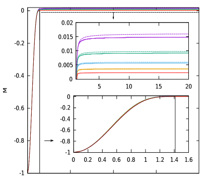
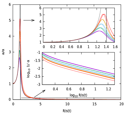
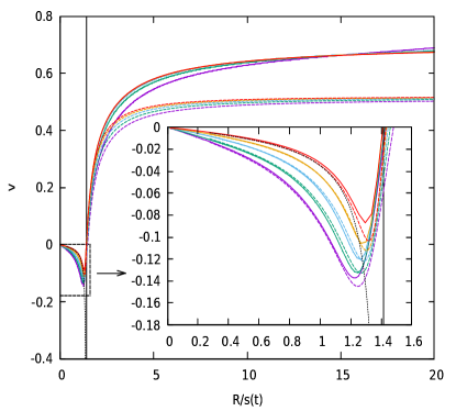
Figure 7: Numerical solution (solid colored lines) for $M$, $s^{2}\rho$, $a/\alpha$, and $v$, plotted against $R/(s(t)$, at different times during the critical regime, $t\simeq 1.1$, $1.3$, $1.5$, $1.7$, and $1.9$. We have made a fit for $s_{0}$ and $\nu$ in $s(t)=s_{0}e^{-\nu t/\ell}$. For comparison, we plot the leading-order term of the quasistatic $\Lambda=0$ solution (black dotted line) and the $\Lambda<0$ solution (colored dotted lines). The vertical black line corresponds to the location of the surface in the $\Lambda=0$ exact static solution. For $\Lambda<0$, there is no sharp surface.

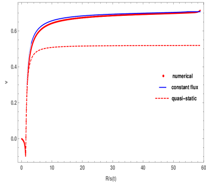
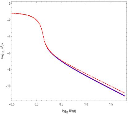
Figure 8: We compare the agreement between the numerical solution for our best subcritical data at $t=1.9$ (red line), the quasistatic solution (dashed line), and the test fluid solution (blue line) on the entire numerical grid. The quasistatic solution underestimates the asymptotic value of the velocity, as well as the rate of decay of the density, (see also Fig. 7), while the constant flux solution correctly predicts these. The small upturn in $v$ just inside the numerical outer boundary is believed to be an effect of the unphysical outer boundary condition.

In Fig. 9, we plot the products $M_{\text{OB}}(t)\rho_{0}(t)$ and $M_{v}(t)\rho_{0}(t)$, where $M_{v}$ is the mass at $R_{v}(t)$, at different levels of fine-tuning. The static solution has the property that in the limit where $s\to 0$, the product $\check{M}_{\infty}\check{\rho}_{0}$ is a constant; see Eq. (84). We then expect the product $M_{\text{OB}}(t)\rho_{0}(t)$ to approach this constant as the solution contracts, $s(t)\to 0$, where we consider $M_{\text{OB}}(t)$ as a substitute for the total mass of the static solution. We find that during the critical regime, the product $M_{\text{OB}}(t)\rho_{0}(t)$ is close to this theoretical value, although in our best subcritical data it eventually becomes larger at the end of the critical regime.

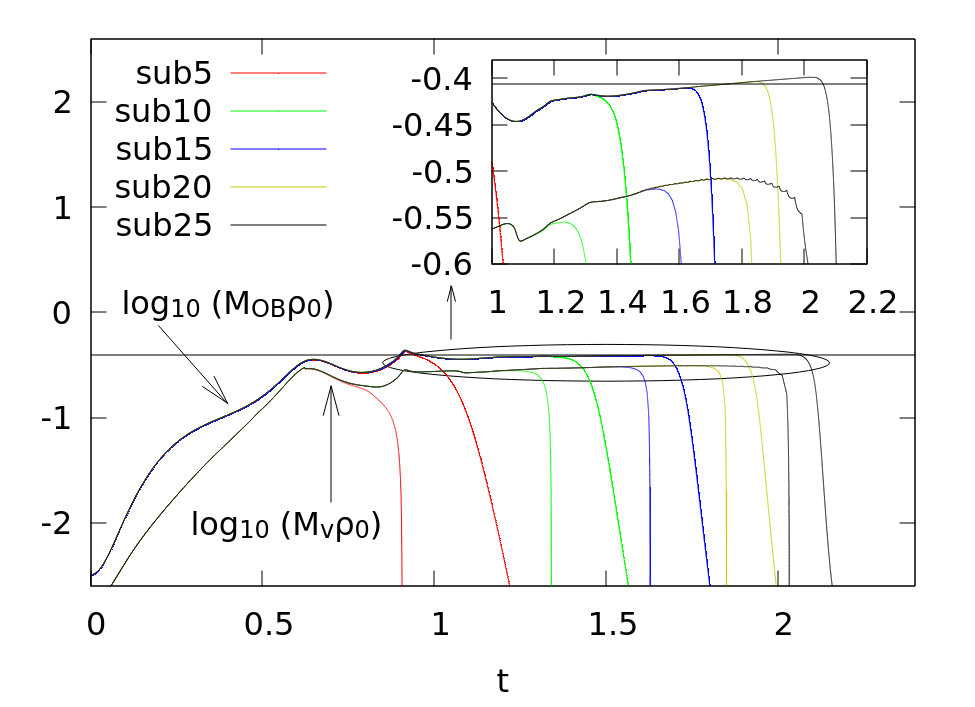
Figure 9: Log plot of $\rho_{0}(t)M_{\text{OB}}(t)$, $\rho_{0}(t)M_{v}(t)$ for sub5 to sub25 data. The black horizontal line corresponds to $\log_{10}\left(\check{M}_{\infty}\check{\rho}_{0}\right)$ and shows that $M_{\text{OB}}(t)$ is a good approximation for the total mass of the corresponding static solution.

In Fig. 10, we compare the fitted scale function $s(t)$ with the observed functions $R_{v}(t)$, $R_{M}(t)$ and $\rho_{0}(t)$, $M_{\text{OB}}(t)$. We find that $x_{\star}s(t)$ approximately matches $R_{v}(t)$ in the critical regime, although the plot also suggests that $R_{M}\to x_{\star}s(t)$, very slowly. $s(t)$ also matches $R_{M}(t)$ and $\rho_{0}(t)M_{\text{OB}}(t)$, up to constant factors.

We also see that $R_{v}\simeq s(t)\check{x}_{c}$, which suggests that $R_{v}\simeq R_{\text{AH}}$ for supercritical data.

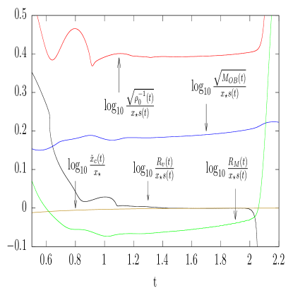
Figure 10: For sub25 data, we compare the values of $R_{M}(t)$, $R_{v}(t)$, $\rho_{0}(t)$, and $M_{\text{OB}}(t)$ with $x_{\star}s(t)$ and $\check{x}_{c}(t)$, where $s(t)$ is the exponential function fitted to the numerical data in Fig. 7.

Finally, in Fig. 11, we provide some evidence for universality of the critical solution by plotting the numerical solution at a fixed time for different initial data. We plot the profiles of $M$, $\alpha$, $R^{2}\rho$, and $v$ for sub25 off-centered, centered and ingoing initial data with $\tilde{\mu}=0.1$. Since $t_{\#}$ depends on the initial data, these three solutions were plotted at different times, namely $t\simeq 1.80$, $1.67$, and $1.74$, respectively, so that the profiles match up.

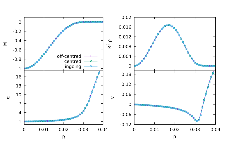
Figure 11: The profiles of $M$, $R^{2}\rho$, $\alpha$, and $v$ in the critical intermediate attractor solution for three different sub25 initial data, giving some evidence for universality. The data have been plotted at times $t\simeq 1.80$, $1.67$, and $1.74$, respectively, chosen to align them.

III.4.3 Derivation of scaling laws

In this section, we provide for a theoretical understanding of the observed law [Eq. (39)].

Motivated by our numerical results, we assume that the critical solution can, to leading order, be modeled as a quasistatic solution, $\check{Z}$; see Appendix C.

For this discussion, two properties of the family of static solution are of importance: First, the central density scales like $\check{\rho}_{0}\sim\ell^{-2}\sim s^{-2}$; see Eq. (69). Second, the total mass of the system, assuming small $\mu\ll 1$, scales like $\check{M}_{\infty}\sim\mu\sim s^{2}$; see Eq. (81).

Since the maximum of the curvature is attained at the center, we can approximate

$$\rho_{\text{max}}\simeq\rho_{0,\text{evolved}}(t_{\#})\simeq\check{\rho}_{0}(-\Lambda s(t_{\#})^{2}).$$ (47)

On the other hand, unlike for the density, one cannot simply make the approximation $M_{\text{AH}}\simeq M_{\infty}\simeq\check{M}_{\infty}$, since the total mass of the system is time independent and therefore cannot scale.

However, our numerical outer boundary does allow mass to escape. Moreover, we have seen that in the region from the surface of the shrinking star to the outer boundary, $M(t,r)$ is approximately constant in $r$ and decreasing adiabatically in time, and that this observation does not depend on the location of the numerical outer boundary. We therefore conjecture that this atmosphere of constant mass flux is physical.

Somewhere further out, and beyond our numerical outer boundary, we would of course find enough mass to bring $M_{\infty}$ to its time-independent value.

In the intermediate regime, between $R_{v}(t)$ (the point beyond which $M$ is approximately constant in space) and the outer boundary $M_{\text{OB}}$, we can then approximate

$$M_{\text{intm.}}(t,R)\simeq\check{M}_{\infty}\left(-\Lambda s(t)^{2}\right)\sim s(t)^{2}.$$ (48)

As the black hole must form with $M>0$, and $M>0$ holds only in the intermediate regime, not inside the star, it follows that $R_{\text{AH}}>R_{M}(t)$. Furthermore, recall that from Fig. 10, in the critical regime $\check{x}_{c}(t)\simeq R_{v}(t)$, implying that $R_{v}(t_{\#})\simeq R_{\text{AH}}$. It is then natural to assume that $M_{\text{AH}}$ takes the above value, evaluated at $t_{\#}$. That is,

$$M_{\text{AH}}\simeq M_{\text{intm.}}(t_{\#},R_{\text{AH}})\sim s(t_{\#})^{-2}.$$ (49)

Taking both approximations for $\rho_{\text{max}}$ and $M_{\text{AH}}$ in terms of $\check{\rho}_{0}$ and $\check{M}_{\infty}$ together into Eq. (84), we then infer the relation in Eq. (39).

This analysis also allows us to predict that $\mathcal{C}=(4\pi(1-\kappa))^{-1}$. For $\kappa=0.5$, this gives $\mathcal{C}\simeq 0.16$, which is consistent with the numerical result; see Table 3.

III.5 Type I-II transition

For arbitrarily good fine-tuning, the type II apparent horizon mass becomes vanishingly small, while the type I mass is a family-dependent constant. In the region between $\kappa=0.43$ and $\kappa=0.5$, type II phenomena are still observed (see Fig. 12), but this is already a transition from type I to type II.

In Fig. 13, we compare the agreement between the quasistatic solution and the numerical results for $\check{v}_{1}$ for $\kappa=0.47$ and $0.54$, plotted at times $t=1.3$, $1.45$, $1.6$, $1.75$, $1.9$ and $t=0.9$, $1.0$, $1.1$, $1.2$, $1.25$, respectively.

For $\kappa=0.54$, we find good agreement between the numerical time evolution and the quasistatic approximation inside the star. For $\kappa=0.47$, we find much poorer agreement, even near the center. As for the $\kappa=0.5$ case, the test fluid solution is a much better model for the atmosphere of the critical solution for both $\kappa=0.54$ and $0.47$; see Fig. 14.

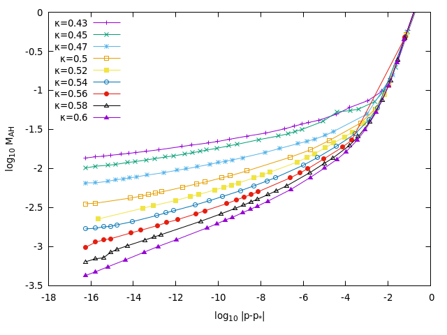
Figure 12: Apparent horizon mass scaling for different values of $\kappa\geq 0.43$. We find typical type II scaling. In all cases, the relation $\delta=2\gamma$ is verified. Compare the equivalent (but flat) scaling laws for $\kappa\leq 0.42$ in Fig. 1.

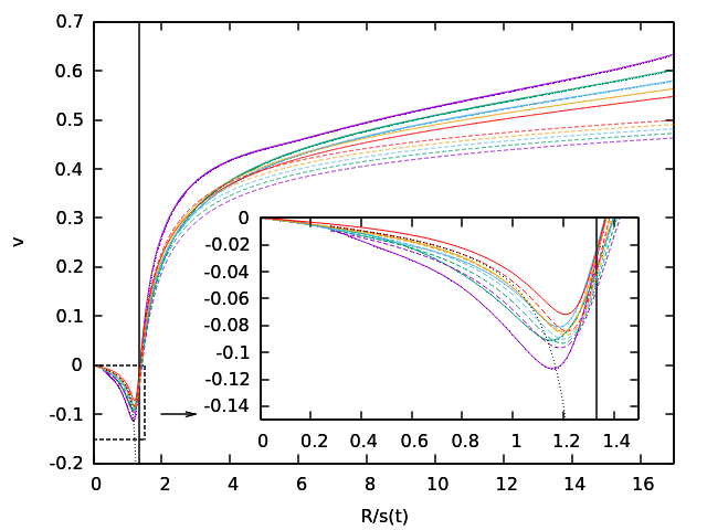
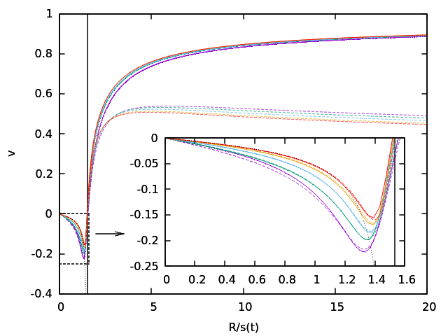
Figure 13: Comparison of the analytical and numerical expressions of $\check{v}_{1}$ for $\kappa=0.47$ (left) and $\kappa=0.54$ (right). The colored (dotted) lines follow a similar convention to Fig. 7.

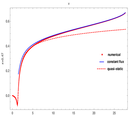
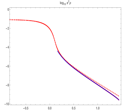
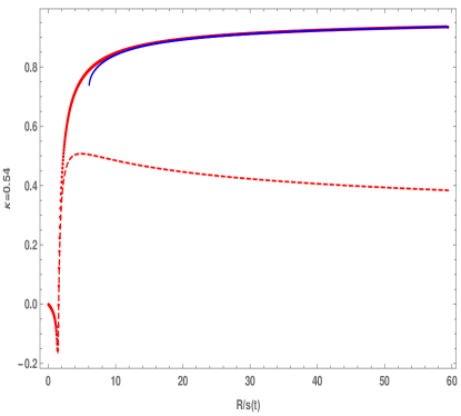
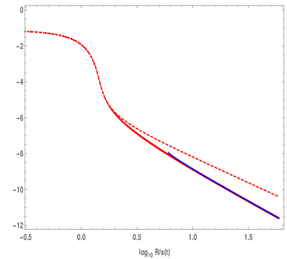
Figure 14: We compare the agreement between the numerical solution (red line), the quasistatic solution (dashed line), and the test fluid solution (blue line) for $\kappa=0.47$ (top two plots) and $\kappa=0.54$ (bottom two plots) for our best subcritical data at $t=1.9$ and $1.25$, respectively. Otherwise, as in Fig. 8.

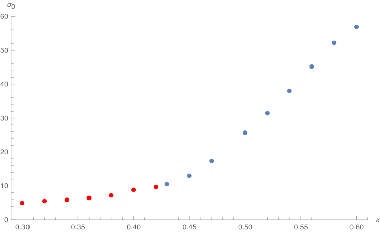
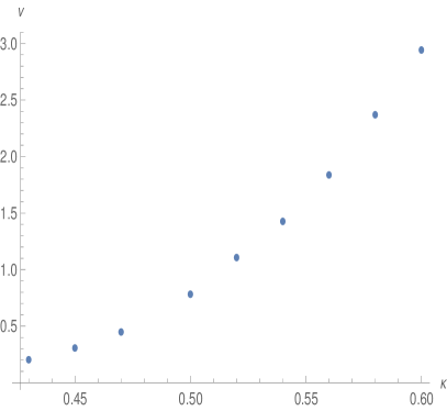
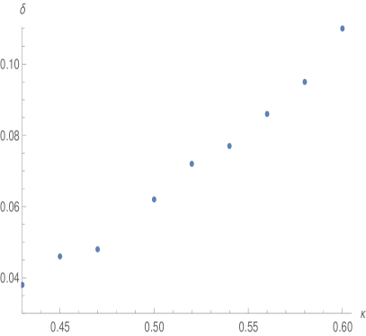
Figure 15: Plot of $\sigma_{0}$ (top), $\nu$ (bottom left) and $\delta$ (bottom right) against $\kappa$. We note that $\sigma_{0}$ appears to be continuous across the type I (red) to type II (blue) transition.

The exponential time dependence of the growing mode holds for both type I phenomena, where $s$ is constant, and type II phenomena, where $s(t)$ is itself exponential. In the case of type II,

$$\text{growing mode}\sim e^{\sigma_{0}t\over\ell}\sim s(t)^{-\lambda_{0}}\sim\left(e^{-{\nu t\over\ell}}\right)^{-\lambda_{0}},$$ (50)

and so we can express $\sigma_{0}$ in terms of $\lambda_{0}$ [Eq. (35)] (or $\gamma$) and $\nu$ [Eq. (46)] as

$$\sigma_{0}=\nu\lambda_{0},$$ (51)

and hence, with $\delta=2/\lambda_{0}$,

$$\delta={2\nu\over\sigma_{0}}.$$ (52)

In Table 4, we give $\nu$, $\delta$, and $\sigma_{0}$ for different values of $\kappa$, and Eq. (52) is explicitly verified. The exponent $\sigma_{0}$ for the exponentially shrinking critical solution is computed in the same way as in the type I case.

Given that $\sigma_{0}$ is defined both in the type I and type II regimes of $\kappa$, one may ask if it is a smooth or at least continuous function of $\kappa$ across both regimes. In Fig. 15, we plot $\sigma_{0}$ (top), $\nu$ (bottom left), and $\delta$ (bottom right) against $\kappa$. The data points are given in Tables 2 and 4. We find that $\nu$ and $\delta$ are monotonically increasing functions of $\kappa$. For $0.3\leq\kappa\leq 0.42$ and $0.5\leq\kappa\leq 0.6$, $\sigma_{0}$ depends linearly on $\kappa$. Due to shocks occurring for $\kappa\leq 0.42$ and causing a systematic error in the evaluation of $\sigma_{0}$ when we use a second-order limiter, the bisections and evolutions were performed using the Godunov limiter. We find that $\sigma_{0}$ is at least continuous in the transition from type I to type II phenomena.

Our plots are compatible with $\delta$ vanishing at $\kappa\simeq 0.42$ because $\nu$ vanishes there, while $\sigma_{0}$ remains finite. In other words, the unstable mode grows exponentially in time in the type I and type II critical solution, but this gives rise to type II mass and curvature power-law scaling only when the critical solution shrinks, also exponentially in time. At the transition from type II to type I in the equation-of-state parameter $\kappa$, the critical solution simply stops shrinking as $\nu(\kappa)\to 0$.

$\kappa$	$\nu$	$\delta$	$\sigma_{0}$	$\frac{\delta\sigma_{0}}{2\nu}$
$0.43$	0.203	0.038	10.54	0.99
$0.45$	0.307	0.046	13.03	0.98
$0.47$	0.448	0.048	17.30	0.93
$0.50$	0.782	0.062	25.69	1.02
$0.52$	1.107	0.072	31.47	1.02
$0.54$	1.427	0.077	38.01	1.03
$0.56$	1.838	0.086	45.21	1.06
$0.58$	2.370	0.095	52.27	1.05
$0.60$	2.943	0.110	56.88	1.06

Table 4: The values of $\nu$, $\delta$, and $\sigma_{0}$ as functions of $\kappa$. In type II, $\nu$ is obtained directly from the critical solution observed in our closest-to-critical time evolutions. As in type I, we have obtained $\sigma_{0}$ from the lifetime scaling [Eq. (30)] of the critical solution.

IV Conclusions

Critical collapse in 2+1 dimensions is an intriguing toy model for 3+1 dimensions, as in 2+1 dimensions axisymmetric solutions depend only on radius and time, making the simulation of rotating collapse as cheap as that of nonrotating collapse. By contrast, one expects complications from the fact that the existence and formation of black holes in 2+1 requires $\Lambda<0$, which breaks the scale-invariance necessary for type II critical phenomena.

In our time evolutions of one-parameter families of initial data, for $\kappa\lesssim 0.42$ we find type I critical collapse: the maximum curvature and apparent horizon mass are constant beyond a certain level of fine-tuning. The critical solution is static, and the time for which it is observed scales as the logarithm of distance to the threshold of collapse.

For $\kappa\gtrsim 0.43$, we find type II critical collapse: At the threshold of (prompt) collapse, the maximum curvature diverges and the apparent horizon mass goes to zero. However, in contrast to 3+1 and higher dimensions, and even to scalar field collapse in 2+1, we find that the corresponding critical solution near the center is not self-similar, but quasistatic, moving through a family of regular static solutions of finite mass with scale parameter $s(t)$. Outside the central slowly shrinking star, the critical solution is better approximated as a test fluid in a background BTZ spacetime with $M\gtrsim 0$, moving mass away from the shrinking star at relativistic speeds.

The only other case of a critical solution at the boundary between blowup and dispersion that is quasistatic known to us is for a spherically symmetric ansatz for the Yang-Mills equations in 4+1 dimensions in flat spacetime (the critical dimension for that system, as 2+1 is for gravity). However, we have not been able to derive the observed exponential form of $s(t)$ from first principles along the lines of Refs. [14, 15].

However, there are also interesting parallels, not yet sufficiently understood, with the self-similar critical solution in 2+1 spherically symmetric scalar field collapse [5]. The critical solution in both 2+1-dimensional systems has a clear separation between a contracting inner region where $M$ increases from $-1$ at the regular center to a very small positive value at the boundary of the shrinking central region, and an outer region, where $M$ remains approximately constant and the matter is purely outgoing.

We have tentatively derived the type II mass scaling law $\delta=2\gamma$ from the observation that the mass in the atmosphere of the quasistatic critical solution scales as $M(t)\sim-\Lambda s(t)^{2}$, and the natural assumption that the apparent horizon mass is given by this mass at the moment when the evolution leaves the critical solution.

In summary, general relativity finds a way of making arbitrarily large curvature and arbitrarily small black holes at the threshold of collapse, even in 2+1 spacetime dimensions. It has to do this in ingenious ways quite differently from 3+1 and higher dimensions. Moreover, it does so very differently for the perfect fluid with ultrarelativistic equation of state $P=\kappa\rho$ (for $\kappa\gtrsim 0.43$) and the massless scalar field [5].

Appendix A No CSS solution for perfect fluid in $2+1$

We show here that in $2+1$ there are no nontrivial self-similar, spherically symmetric perfect fluid solutions with a barotropic equation of state, $P=\kappa\rho$, that is regular at the light cone.

We employ a similar notation as in Ref. [13] namely, the independent variables are defined by

$$x:=-{r\over t},\quad\tau:=-\ln(-t)$$ (53)

and

$$N:=\frac{\alpha}{ax},\,A:=a^{2},\,\omega:=4\pi r^{2}a^{2}\rho.$$ (54)

The equations of motion read

$${A^{\prime}\over A} =\frac{4\omega(1+v^{2}\kappa)}{x(1-v^{2})},$$ (55)

$${\omega^{\prime}\over\omega} =$$

$$\frac{\left(1+v^{2}\kappa\right)\left(\left(1-\kappa\right)\left(v^{2}(2\omega+1)+2\omega\right)+2\right)}{x\left(1-v^{2}\right)\left(1-v^{2}\kappa\right)},$$ (56)

$${v^{\prime}\over v} =\frac{(1+v^{2}\kappa)(1+2\omega(1-\kappa))}{x(1-v^{2}\kappa)},$$ (57)

$$N =-\frac{1+\kappa v^{2}}{v(1+\kappa)}.$$ (58)

It is important to notice that the velocity is restricted to negative values $-1<v<0$ and $A^{\prime}\geq 0$, $\omega^{\prime}\geq 0$, and $v^{\prime}\leq 0$.

By definition, the light cone, $x=x_{\text{lc}}$, occurs at $v^{2}(x_{\text{lc}})=1$.

First, we show that $x_{\text{lc}}$ is finite. From Eq. (57), we can find an upper bound for $|v|^{\prime}$,

$${|v|^{\prime}\over|v|}\geq\frac{1+v^{2}\kappa}{x(1-v^{2}\kappa)}.$$ (59)

The above inequality is separable and upon integration we find

$$x\leq\frac{C|v|}{1+\kappa v^{2}},$$ (60)

where $C>0$ is an integration constant. In particular, we find an upper bound for $x_{\text{lc}}$,

$$x_{\text{lc}}\leq\frac{C}{1+\kappa}<\infty.$$ (61)

Since $x_{\text{lc}}$ is finite, the ODE system needs to be regularized at that point. Specifically, we must impose the numerators in Eqs. (55) and (56) to vanish at the light cone, which gives the constraint

$$\omega(x_{\text{lc}})=0.$$ (62)

This constraint, together with the property that $\omega^{\prime}\geq 0$, implies

$$\omega(x)=0,\qquad x\in[0,x_{\text{lc}}],$$ (63)

which proves our claim.

Appendix B Spherically symmetric static fluid

We review here the relevant properties of the static perfect fluid solutions with $\Lambda\leq 0$. We refer the reader to Ref. [11] for a more complete discussion.

For a given equation of state, these can be parameterized by a length scale $s$, so that formally we can write

$$Z=\hat{Z}(R,s),\qquad Z:=\{R^{2}\rho,a,\alpha,M\},$$ (64)

where the hat denotes the static solution, when expressed in terms of the radial coordinate $R$ and scale parameter $s$. (We come back to the interpretation of $s$ below).

The functions $\hat{Z}(R,s)$ cannot be given in closed form, but the quantities $Z$ and the area radius $R$ can be given explicitly in terms of an auxiliary radial coordinate $y$ that is defined by $\alpha=:y$.

We introduce the intermediate dimensionless quantities

$$x:={R\over s}$$ (65)

and

$$\mu:=-\Lambda s^{2}.$$ (66)

We can then write

$$\hat{Z}=\check{Z}(x,\mu),\qquad\check{R}=\sqrt{\mu}\ell x.$$ (67)

We then have the following explicit expressions for the static solution, but expressed in terms of the radial coordinate $y$ and parameter $\mu$:

$$\bar{\alpha} =: y,$$ (68)

$$\bar{\rho} = {1-\mu\over 8\pi\kappa\mu\ell^{2}}y^{-{1+\kappa\over\kappa}},$$ (69)

$$\bar{a}^{-1} = \mu y+(1-\mu)y^{-{1\over\kappa}},$$ (70)

$$\bar{M} = \bar{x}^{2}\mu-\bar{a}^{-2},$$ (71)

$$\bar{x}^{2} = \mu(y^{2}-1)+{2\kappa(1-\mu)\over 1-\kappa}\left(1-y^{-{1-\kappa\over\kappa}}\right).$$

(72)

$$\bar{R} = \sqrt{\mu}\ell\bar{x}.$$ (73)

The functions $\hat{Z}(R,s)$ are now given implicitly in terms of $\bar{R}(y,\mu)$ and $\bar{Z}(y,\mu)$.

Note that only values $0\leq\mu\leq 1$ are physical, that $R=0$ is at $y=1$, and that (for $\mu>0$ only) $R\to\infty$ as $y\to\infty$.

We also need to evaluate $\hat{Z}_{,R}$ and $\hat{Z}_{,s}$. For these, we can derive the following expressions that are explicit in $y$ and $\mu$:

$$\hat{Z}_{,s} = {2\over\ell\sqrt{\mu}}\left(\mu\bar{Z}_{,\mu}-{\mu(\bar{x}^{2})_{,\mu}+\bar{x}^{2}\over(\bar{x}^{2})_{,y}}\bar{Z}_{,y}\right),$$

$$\hat{Z}_{,R} = {2\bar{x}\over\ell\sqrt{\mu}(\bar{x}^{2})_{,y}}\bar{Z}_{,y}.$$ (75)

For $\mu\ll 1$, we can distinguish a stellar interior and an atmosphere, divided by a sharp turning point in $\hat{\rho}(R,s)$. While the surface of the star is not defined precisely in the presence of an atmosphere, we can take it to be at

$$y=y_{c}:=\left(1-\mu\over\kappa\mu\right)^{\kappa\over 1+\kappa},$$ (76)

which marks both the maximum of $\bar{a}$ and the turning point of $\bar{x}^{2}$, with respect to $y$. Note that for $\mu\ll 1$,

$$\bar{x}(y_{c},\mu)=:\check{x}_{c}\simeq x_{\star}$$ (77)

In the interior of the star we can neglect the first term in $\bar{x}^{2}$, obtaining the approximate closed-form expression for $\check{y}$,

$$\check{y}\simeq\left(1-{1\over 1-\mu}{x^{2}\over x_{\star}^{2}}\right)^{-{\kappa\over 1-\kappa}},$$ (78)

where we have defined

$$x_{\star}^{2}:={2\kappa\over 1-\kappa}.$$ (79)

Explicit approximate expressions for $\check{Z}$ then follow.

In the exterior of the star, we can approximate the second term in $\bar{x}^{2}$ by its asymptotic value, obtaining

$$\check{y}\simeq\mu^{-1}\left(-\check{M}_{\infty}+\mu x^{2}\right)^{1\over 2}=\mu^{-1}\left(-\check{M}_{\infty}+{\check{R}^{2}\over\ell^{2}}\right)^{1\over 2},$$ (80)

where

$$\check{M}_{\infty}:={-(1+\kappa)\mu^{2}+2\kappa\mu\over 1-\kappa},$$ (81)

is the total mass of the system. This again gives explicit approximate expressions for $\check{Z}$, in particular

$$\mu^{2}\check{\alpha}^{2}\simeq\check{a}^{-2}\simeq-\check{M}_{\infty}+{\check{R}^{2}\over\ell^{2}}.$$ (82)

We see that in the atmosphere, the metric is approximated by the BTZ metric with fixed mass $\check{M}_{\infty}$ (and $t$ rescaled relative to the convention for BTZ solutions), and so the fluid is approximated as a test fluid, neglecting its self-gravity.

Substituting Eq. (80) into Eq. (69), we find

$$\check{\rho}\simeq{1-\mu\over 8\pi\kappa\mu\ell^{2}}\left(-{\check{M}_{\infty}\over\mu}+x^{2}\right)^{-{1+\kappa\over 2\kappa}}.$$ (83)

The central density $\check{\rho}_{0}:=\check{\rho}(0,\mu)$ is related to the total mass by

$$\lim\limits_{\mu\to 0}{\check{M}_{\infty}\check{\rho}_{0}\over-\Lambda}=\frac{1}{4\pi(1-\kappa)}.$$ (84)

We now come back to the interpretation of $s$ as a length scale. For $0<\mu\ll 1$, the surface $y=y_{c}$ is at $x\simeq x_{\star}$, and hence at $R\simeq x_{\star}s$. In this sense, $x_{\star}s$ is the size of the star. In the limiting case $\mu=0$, the star has a sharp surface at $x=x_{\star}$, with $\check{M}_{\infty}=0$ in the vacuum exterior. The exterior spatial geometry is then that of a cylinder of constant radius. The limit $\mu\to 0$ is singular in the sense that for vanishing $\mu$, the approximation $\check{Z}(x,\mu)\simeq\check{Z}(x,0)$ is only valid for $x<x_{\star}$.

This means that in the limit where the size of the star is small compared to the cosmological length scale $\ell$, $\mu=s^{2}/\ell^{2}\ll 1$, the family of static solutions becomes invariant under rescaling $R$ and $\rho$ according to their dimensions, but only in the interior of the star. In the atmosphere, $Z=\check{Z}(x,0)$ is not a good approximation for small but finite $\mu$, and we need the full form $Z=\check{Z}(x,\mu)$.

Appendix C The quasi-static solution

We model the critical solution as quasistatic, meaning that it adiabatically goes through the sequence of static solutions, with $s$ now a function of $t$, and $|\dot{s}(t)|\ll 1$. We can then formally expand the quantities $Z$ in even powers of $\dot{s}$, and $v$ in odd powers.

In fact, from the exponential form of $s(t)$ [Eq. 46], it follows that $\dot{s}=-\nu s/\ell=-\nu\sqrt{\mu}$, and hence $\dot{s}^{2}=s\ddot{s}=\nu^{2}\mu$, and so the quasistatic approximation is equivalent to the small-$\nu$ approximation. For now, however, we do not assume the exponential form.

The leading and next order for $Z$ in the quasistatic ansatz are

$$Z_{\star}(R,t)=Z_{0}(R,t)+\dot{s}^{2}(t)Z_{2}(R,t)+O(\dot{s}^{4}),$$ (85)

where

$$Z_{0}(R,t):=\hat{Z}(R,s(t)).$$ (86)

As noted above, we do not have $\hat{Z}(R,s)$ in explicit form, only $\bar{Z}(y,\mu)$. For the velocity, we make the ansatz

$$u_{\star}(R,t)=\dot{s}(t)u_{1}(R,t)+O(\dot{s}^{3}),$$ (87)

where we have defined

$$u:=\Gamma^{2}v={v\over 1-v^{2}}.$$ (88)

Clearly, for small $\dot{s}$ we have

$$v_{\star}(R,t)=\dot{s}(t)u_{1}+O(\dot{s}^{3}),$$ (89)

but expanding $u$ rather than $v$ in a series in $\dot{s}$ makes sure that $|v|<1$.

To order $\dot{s}$, the Einstein equation (21) becomes

$$M_{{0},t}=\dot{s}\hat{M}_{,s}\simeq-16\pi f_{\Omega}.$$ (90)

This gives

$$\hat{u}_{1}:=-{\hat{a}\hat{M}_{,s}\over 16\pi(1+\kappa)R\hat{\rho}\hat{\alpha}}.$$ (91)

As for $\hat{Z}$, we can compute $\bar{u}_{1}(y,\mu)$ explicitly, and as expected, we find that $\check{u}_{1}(x,\mu)\simeq\check{u}_{1}(x,0)$ for $x<x_{\star}$. However, $\check{u}_{1}(x,0)$ blows up at the surface $x=x_{\star}$, while $\check{u}_{1}(x,\mu)$ is regular for all $x$.

As $R\to\infty$, $u_{1}$ goes to zero for $\kappa>1/2$, approaches a constant value for $\kappa=1/2$, and diverges for $\kappa<1/2$. Hence, the expansion in $\dot{s}$ breaks down in the atmosphere for $\kappa<1/2$ at sufficiently large radius $R$ and contraction speed $|\dot{s}|$. However, for the values of $\dot{s}$ for which we show plots, this is not a problem for values of $R$ on our numerical grid.

The momentum balance law is obeyed to leading order in $\dot{s}^{2}$ by construction. Going to the next order, we see that the $Y_{,t}$ term, with $Y\propto u_{1}\dot{s}$, produces a term proportional to $\ddot{s}$.We consider $s\ddot{s}$ as the same order as $\dot{s}^{2}$, which is true when $s(t)$ is either exponential or a power.

The ansatz

$$s\ddot{s}=G(\mu)\dot{s}^{2}$$ (92)

results in an inhomogeneous first-order ODE in $y$ for $\rho_{2}$, with $\mu$ merely a parameter, and no explicit appearance of $s(t)$ or $t$ derivatives, and so can be thought of as a separation of variables ansatz.

This ODE in $y$ for $\rho_{2}$ contains $a_{2}$, although $\alpha_{2}$ drops out when we use the background momentum balance law. To close the system, we must perturb therefore only the Einstein equation (20) to $\mathcal{O}(\dot{s}^{2})$ to get an ODE for $a_{2}$.

The resulting system of two inhomogeneous first-order ODEs in $y$ for $\rho_{2}$ and $a_{2}$ can also be rewritten as a single second-order inhomogeneous ODE for $M_{2}$. Obviously, the solutions of the corresponding homogeneous ODE, obtained by setting $u_{1}=0$, are simply the static perturbations of the regular static solution. One of these is singular at the origin and so is ruled out by regularity. The other, with $M_{2}=0$ at the origin and finite at infinity, is the infinitesimal change $\hat{M}_{,s}$ from one regular static solution to a neighboring one.

We had hoped to find a natural boundary condition for $M_{2}$ at infinity that would select the value $G(\mu)=1$ of the separation constant, in order to predict the observed exponential form of $s(t)$. This would have been similar in spirit to the approach of Ref. [14] for a quasistatic critical solution (in Yang-Mills on flat spacetime in 4+1 dimensions).

However, we have not found such a boundary condition. In particular, $M_{2}$ is finite at $R=\infty$ (and can then be set to zero there by adding a multiple of $\hat{M}_{,s}$) for all $\kappa\geq 1/2$, but for all $\kappa<1/3$, it blows up at $R=\infty$, with $G(\mu)$ only affecting lower-order terms. For $1/3<\kappa<1/2$, $M_{2}$ is finite, but since $u_{1}$ is not, the quasistatic ansatz is also not valid in this case, as $\dot{s}u_{1}$ can then not be considered as small.

Appendix D Stationary test fluid solutions

To understand better what happens for $\kappa\leq 1/2$, where $u_{1}$ diverges at infinity, we note that the fluid in the atmosphere can be approximated as a test fluid on a fixed BTZ spacetime with mass $\check{M}_{\infty}$.

The solutions describing a stationary test fluid with constant mass flux on a BTZ spacetime with mass $M$ can be given in implicit form as

$$v(1-v^{2})^{1-\kappa\over 2\kappa} = {f_{\Omega}\over C\rho_{0}(1+\kappa)}{(-M-\Lambda R^{2})^{1-\kappa\over 2\kappa}\over R}$$

$$\rho = \rho_{0}(-M-\Lambda R^{2})^{-{1+\kappa\over 2\kappa}}(1-v^{2})^{1+\kappa\over 2\kappa}.$$

Here, the free parameter $f_{\Omega}$ is the constant mass flux, $C:=a\alpha$ is a constant in vacuum that depends on the normalization of the time coordinate $t$, and the free parameter $\rho_{0}$ is an overall factor in $\rho$ chosen so that it is the density at the center in the static solution on AdS spacetime.

We note that generically, Eq. (D) has either two solutions $v$ or none. From

$$v(1-v^{2})^{1-\kappa\over 2\kappa}\sim R^{1-2\kappa\over\kappa},$$ (95)

we see that for $\kappa>1/2$, either $v\to 0$ or $v\to\pm 1$ as $R\to\infty$. The $v\to 1$ solution is the one relevant for our critical solution. We then have

$$\rho\sim R^{-{1+\kappa\over 1-\kappa}}.$$ (96)

However, for $\kappa<1/2$, the right-hand side of Eq. (D) increases with $R$, and so $v$ is defined only up to some maximum value of $R$, beyond which the constant flux solution does not exist (for given $f_{\Omega}$ and $\rho_{0}$).

In the top two plots of Fig. 14, we show that this ansatz for $\kappa=0.47$ is in good agreement with our numerical solution up to the numerical outer boundary. The radius after which $v$ is not defined as explained above lies outside our numerical grid.

References

- [1] M. W. Choptuik, Universality and scaling in gravitational collapse of a massless scalar field, Phys. Rev. Lett. 70, 9 (1993).
- [2] C. Gundlach and J. M. Martin-García, Critical Phenomena in Gravitational Collapse, Liv. Rev. Relativity 10, 5 (2007).
- [3] J. Jałmużna and C. Gundlach, Critical collapse of a rotating scalar field in dimensions, Phys. Rev. D 95, 084001 (2017).
- [4] F. Pretorius and M. W. Choptuik, Gravitational collapse in dimensional AdS spacetime, Phys. Rev. D. 62, 12 (2000).
- [5] J. Jałmużna, C. Gundlach and T. Chmaj, Scalar field critical collapse in dimensions, Phys. Rev. D 92, 12 (2015).
- [6] C. Gundlach, P. Bourg and A. Davey, A fully constrained, high-resolution shock-capturing, formulation of the Einstein-fluid equations in dimensions, arXiv:2103.04435 [gr-qc] (2021).
- [7] M. Bañados, C. Teitelboim, and J. Zanelli, Black Hole in Three-Dimensional Spacetime, Phys. Rev. Lett. 69, 13 (1992).
- [8] P. Bizoń and A. Rostworowski, Weakly turbulent instability of anti-de Sitter space, Phys. Rev. Lett. 107, 031102 (2011).
- [9] R. J. LeVeque, Finite Volume Methods for Hyperbolic Problems, Cambridge University Press (2002).
- [10] M. Cataldo, Rotating perfect fluids in (2+1)-dimensional Einstein gravity, Phys. Rev. D 69, 064015 (2004).
- [11] C. Gundlach and P. Bourg, Rigidly rotating perfect fluid star in dimensions, Phys. Rev. D 102, 084023 (2020).
- [12] C.R. Evans and J.S. Coleman, Critical Phenomena and Self-Similarity in the Gravitational Collapse of Radiation Fluid, Phys. Rev. Lett. 72, 1782–1785 (1994).
- [13] T. Hara, T. Koike and S. Adachi, Renormalization group and critical behaviour in gravitational collapse, arXiv:9607010 [gr-qc] (1994).
- [14] P. Bizon, Y. N. Ovchinnikov, and I. M. Sigal, Collapse of an instanton, Nonlinearity 17, 4 (2004).
- [15] I. Rodnianski and J. Sterbenz, On the formation of singularities in the critical -model, Ann. Math. 172, 187 (2010).