Piggyback GAN: Efficient Lifelong Learning for Image Conditioned Generation

Abstract

Humans accumulate knowledge in a lifelong fashion. Modern deep neural networks, on the other hand, are susceptible to catastrophic forgetting: when adapted to perform new tasks, they often fail to preserve their performance on previously learned tasks. Given a sequence of tasks, a naive approach addressing catastrophic forgetting is to train a separate standalone model for each task, which scales the total number of parameters drastically without efficiently utilizing previous models. In contrast, we propose a parameter efficient framework, Piggyback GAN, which learns the current task by building a set of convolutional and deconvolutional filters that are factorized into filters of the models trained on previous tasks. For the current task, our model achieves high generation quality on par with a standalone model at a lower number of parameters. For previous tasks, our model can also preserve generation quality since the filters for previous tasks are not altered. We validate Piggyback GAN on various image-conditioned generation tasks across different domains, and provide qualitative and quantitative results to show that the proposed approach can address catastrophic forgetting effectively and efficiently.

1 Introduction

Humans are lifelong learners: in order to function effectively day-to-day, we acquire and accumulate knowledge throughout our lives. The accumulated knowledge makes us efficient and versatile when we encounter new tasks. In contrast to human learning, modern neural network based learning algorithms usually fail to remember knowledge acquired from previous tasks when adapting to a new task (see Figure LABEL:fig:intro (b)). In other words, it is difficult to generalize once a model is trained on a task. This is the well-known phenomenon of catastrophic forgetting [25]. Recent efforts [32, 20, 6, 2] have demonstrated how discriminative models can continually learn a sequence of tasks. Despite the success of these efforts for discriminative models, lifelong learning for generative models remains a challenging and under-explored area.

Lifelong learning methods for discriminative models cannot be directly applied to generative models due to their intrinsic differences. First, it is well known that in classification tasks, the intermediate convolutional layers in deep neural networks are capable of providing generic features. These features can easily be reused by other models with varying and different classification goals. For generative models, the possibility of such reuse for new generative tasks has not been previously explored, to the best of our knowledge. Second, different from discriminative models, the output space of generative models is usually continuous, making it more challenging for the model to maintain the generation quality along the training of a sequence of tasks. Third, there could be conflicts between tasks under the generative setting. For discriminative models, it rarely happens that one image has different labels (appears in different tasks). However, for generative models, it is quite common that we want to translate the same image to different domains for different tasks [14, 11, 44, 8].

One of the naive approaches to address catastrophic forgetting for generative models is to train a model for each task separately (see Figure LABEL:fig:intro (c)). Unfortunately, this approach is not scalable in general: as new tasks are added, the storage requirements grow drastically. More importantly, setting the trained model aside without exploiting the benefit it can potentially provide facing a new task would be an inefficient use of resources. Recent works [42, 37] have shown promising results on lifelong learning for generative models, but it is also revealed that image quality degradation and artifacts transfer from old to new tasks are inevitable. Therefore, it is valuable to have a continual learning framework designed that (1) is more parameter efficient, (2) preserves the generation quality of both current and previously learned tasks, and (3) can enable various conditional generation tasks across different domains.

In this paper, we introduce a generic continual learning framework Piggyback GAN that can perform various conditional image generation tasks across different domains (see Figure LABEL:fig:intro (d)). The proposed approach addresses the catastrophic forgetting problem in generative continual learning models. Specifically, Piggyback GAN maintains a filter bank, the filters in which come from convolution and deconvolution layers of models trained on previous tasks. Facing a new task, Piggyback GAN learns to perform this task by reusing the filters in the filter bank by building a set of piggyback filters which are factorized into filters from the filter bank. Piggyback GAN also maintains a small portion of unconstrained filters for each task to ensure high-quality generation. Once the new task is learned, the unconstrained filters are appended to the filter bank to facilitate the training of subsequent tasks. Since the filters for the old task have not been altered, Piggyback GAN is capable of keeping the exact knowledge of previous tasks without forgetting any details.

To summarize, our contributions are as follows. We propose a continual learning framework for conditional image generation that is (1) efficient, learning to perform a new task by “piggybacking” on models trained on previous tasks and reusing the filters from previous models, (2) quality-preserving, maintaining the generation quality of current task and ensuring no quality degradation for previous tasks while saving more parameters, and (3) generic, enabling various conditional generation tasks across different domains. To the best of our knowledge, we are the first to make these contributions for generative continual learning models. We validate the effectiveness of our approach under two settings: (1) paired image-conditioned generation, and (2) unpaired image-conditioned generation. Extensive qualitative and quantitative comparisons with state-of-the-art models are carried out to illustrate the capability and efficiency of our proposed framework to learn new generation tasks without the catastrophic forgetting of previous tasks.

2 Related Work

Our work intersects two previously disjoint lines of research: lifelong learning of generative models, and parameter-efficient network learning.

Lifelong learning of generative models. For discriminative tasks, e.g. classification, many works have been proposed recently for solving the problem of catastrophic forgetting. Knowledge distillation based approaches [32, 20, 4] work by minimizing the discrepancy between the output of the old and new network. Regularization-based approaches [19, 5, 2, 6, 22] regularize the network parameters when learning new tasks. Task-based approaches [31, 3, 28] adopt task-specific modules to learn each task.

For generative tasks, lifelong learning is an underexplored area and relatively less work studies the problem of catastrophic forgetting. Continual generative modeling was first introduced by Seff et al. [30], which incorporated the idea of Elastic Weight Consolidation (EWC) [19] into the lifelong learning for GANs. The idea of memory replay, in which images generated from a model trained on previous tasks are combined with the training images for the current task to allow for training of multiple tasks, is well explored by Wu et al. [37] for label-conditioned image generation. However, this approach is limited to label-conditioned image generation and is not applicable for image-conditioned image generation since no ground-truth conditional inputs of previous tasks are provided. EWC [19] has been adapted from classification tasks to generative tasks of label-conditioned image generation [30, 37], but they present limited capability in both remembering previous tasks and generating realistic images. Lifelong GAN [42] is a generic knowledge-distillation based approach for conditioned image generation in lifelong learning. However, the image quality of generated images of previous tasks keeps decreasing when new tasks are learned. Moreover, all approaches mentioned above fail in the scenario when there are conflicts in the input-output space across tasks. To the best of our knowledge, Piggyback GAN is the first method that can preserve the generation quality of previous tasks, and enables various conditional generation tasks across different domains.

Parameter-efficient network learning. In recent years, there has been increasing interest in better aligning the resource consumption of neural networks with the computational constraints of the platforms on which they will be deployed [7, 36, 38]. One important avenue of active research is parameter efficiency. Trained neural networks are typically highly over-parameterized [10]. There are many effective strategies for improving the parameter efficiency of trained networks: for example, pruning algorithms learn to remove redundant or less important parameters [12, 40], and quantization algorithms learn to represent parameters using fewer bits while maintaining task performance [15, 17, 43]. Parameter efficiency can also be encouraged during training via architecture design [23, 29], sparsity inducing priors [33], resource re-allocation [26], or knowledge distillation from a teacher network [34, 41]. Our work is orthogonal to these methods, which may be applied on top of Piggyback GAN.

The focus of this work is parameter-efficient lifelong learning: we aim to leverage weight reuse and adaptation to improve parameter efficiency when extending a trained network to new tasks, while avoiding the catastrophic forgetting of previous tasks. Several approaches have been explored for parameter-efficient lifelong learning in a discriminative setting. For example, progressive networks [28] train a new network for each task and transfer knowledge from previous tasks by learning lateral connections, a linear combination of layer activations from previous tasks is computed and added to the inputs to the corresponding layer of the new task. While our approach computes a linear combination of filters to construct new filters and uses them the same as normal filters. Rebuffi et al. [27] aims to train a universal vector that are shared among all domains providing generic filters for all domains, and task-specific adapter modules are added to adjust the trained network to new tasks. While we are working on solving a sequence of tasks, the filters trained for the initial task are hardly generic enough for later tasks. Inspired by binary neural networks, Mallya et al. [24] introduced the piggyback masking method (which inspired the naming of Piggyback GAN). This method learns a binary mask over the network parameters for each new task. Tasks share the same backbone parameters but differ in the parameters that are enabled. Multi-task attention networks [21] learn soft attention modules for each new task. Task-specific features are obtained by scaling features with an input-dependent soft attention mask. To the best of our knowledge, Piggyback GAN is the first method for parameter-efficient lifelong learning in a generative setting.

3 Method

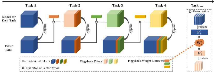
Figure 1: Overview of Piggyback GAN. Piggyback GAN maintains a filter bank for composing convolutional filters to be used for the next task. Given a new task, most filters in the model are trained as piggyback filters that are factorized into filters in the filter bank. The remaining small portion of filters are learned without constraints and appended to the filter bank to benefit the training of subsequent tasks.

In this paper, we study the problem of lifelong learning for generative models. The overall goal is to learn the model for a given sequence of generation tasks $\{T_{i}\}_{i=1}^{N}$ under the assumption that the learning process has access to only one task at a time and training data for each task is accessible only once.

Assume that we have a learnt model $M$ trained to perform the first task $T_{1}$. To proceed with the new task $T_{2}$, one naive approach is to adapt the learnt model $M$ to the new task by fine-tuning its parameters. This approach suffers from the problem of catastrophic forgetting of task $T_{1}$. Another naive approach is to learn a separate standalone model $M_{i}$ for each new task $T_{i}$ and store all learnt models $\{M_{i}\}_{i=1}^{N}$, which drastically scales up total number of parameters without utilizing previous models.

The key idea of this paper is to build a parameter efficient lifelong generative model by “piggybacking” on existing models and reusing the filters from models trained on previous tasks while maintaining the generation quality to be similar to a single standalone model for all tasks. We achieve this by maintaining a filter bank, and compose the filters for new tasks mostly by factorizing it into filters in the filter bank, with a small portion of filters learnt without constraints. Once the new task is learnt, the filter bank is expanded by adding those unconstrained filters.

3.1 Piggyback Filter Learning

For lifelong learning of generative models, given an initial task $T_{1}$ and an upcoming new task $T_{2}$, there could be cases where $T_{1}$ and $T_{2}$ share similar inputs but different outputs, e.g. $T_{1}$ is Photo $\rightarrow$ Monet Paintings and $T_{2}$ is Photo $\rightarrow$ Ukiyo-e Paintings. These conflicts in input-output space do not occur when each task is trained separately. However, as already mentioned, learning a separate model for each task and storing all learnt models is memory consuming and does not utilize previous models.

For this scenario, the knowledge in the filters from the model trained for $T_{1}$ could provide valuable information for the training of $T_{2}$. For images from domains that are less visually similar, it is well known that in discriminative tasks, the generaliziblity of convolutional neural networks helps maintain its capability in previously unseen domains [24, 27]. Such evidence suggests that despite the difference in fine details, certain general patterns that convey semantics could still be covered in previous filter space. Inspired by these observations, we propose to utilize previously trained filters to facilitate the training of new tasks. In our experiments, we do find that previous filters make steady contribution to learning new tasks regardless of the domain difference across tasks.

Consider a generator network $G_{1}$ learnt for initial task $T_{1}$ consisting of $L$ layers of filters $\{F_{1}^{\ell}\}_{\ell=1}^{L}$ where $\ell$ denotes the index of layers. For the ${\ell}^{th}$ layer, let the kernel size be $s_{w}^{\ell}\times s_{h}^{\ell}$, number of input channels be $c_{in}^{\ell}$ and number of output channels be $c_{out}^{\ell}$. Then $F^{\ell}_{1}$ is reshaped from 4D into 2D of size $s_{w}^{\ell}\times s_{h}^{\ell}\times c_{in}^{\ell}$ by $c_{out}^{\ell}$, which we denote by $\mathcal{R}(F^{\ell}_{1})$. For the upcoming task $T_{2}$, we learn the filters $F^{\ell}_{2}$ through factorization operation over filters of the corresponding layers in task $T_{1}$, namely

$$\begin{split}F^{\ell}_{2}\,=\,\mathcal{R}^{-1}(\mathcal{R}(F^{\ell}_{1})\otimes W^{\ell}_{2}),\end{split}$$ (1)

where $\otimes$ denotes the standard matrix multiplication operation and $\mathcal{R}^{-1}$ denotes the inverse of reshape operation from 2D back to 4D. The derived filters $F^{\ell}_{2}$ is denoted as piggyback filters and the corresponding learnable weights $W^{\ell}_{2}\in\mathbb{R}^{c_{out}^{\ell}\times c_{out}^{\ell}}$ is denoted as piggyback weight matrix. The resulting $F^{\ell}_{2}\in\mathbb{R}^{s_{w}^{\ell}\times s_{h}^{\ell}\times c_{in}^{\ell}\times c_{out}^{\ell}}$ is of the same size as $F^{\ell}_{1}$. A bias term could be added to the factorized filters to adjust the final output.

Therefore, by constructing factorized filters, the number of parameters required to be learnt for this layer is reduced from $s_{w}^{\ell}\times s_{h}^{\ell}\times c_{in}^{\ell}\times c_{out}^{\ell}$ to only $c_{out}^{\ell}\times c_{out}^{\ell}$.

3.2 Unconstrained Filter Learning

Parameterizing a new task completely by making use of filters in the initial tasks, though saving substantial storage, cannot capture the key differences between tasks. The filters derived from previous tasks may only characterize certain attributes and may not generalize well to the new task, resulting in poor quality of generation details for the new model. Learning a small number of unconstrained filters gives the model greater flexibility in adapting to the new task. Moreover, learning these unconstrained filters could learn to generate patterns that do not exist in previous tasks, thereby, increasing the power of the model and helping the training of later tasks.

Specifically, for each layer in the generator, we allocate a small portion of unconstrained filters which are learned freely without the constraint to be constructed from previous filters. With a total of $c^{\ell}_{out}$ filters in $F^{\ell}_{2}$, consider the proportion of unconstrained filters to be $\lambda\,(0<\lambda\leq 1)$, then we have $\lambda c^{\ell}_{out}$ unconstrained filters and $(1-\lambda)c^{\ell}_{out}$ piggyback filters, and the size of piggyback weight matrix $W^{\ell}_{2}$ has changed to $c_{out}^{\ell}\times(1-\lambda)c_{out}^{\ell}$. Let the unconstrained filters at the $l^{th}$ layer of the $n^{th}$ task $T_{n}$ be $F_{n}^{u,\ell}$, and piggyback filters at the $l^{th}$ layer of the $n^{th}$ task $T_{n}$ be $F_{n}^{p,\ell}$.

For task $T_{1}$, all filters are unconstrained filters, namely

$$F^{\ell}_{1}\,=\,F^{u,\ell}_{1}.$$ (2)

For task $T_{2}$, we re-define the filters in $F^{2}_{l}$ to be the concatenations of unconstrained filters $F_{2}^{u,\ell}$ and piggyback filters $F_{2}^{p,\ell}$, namely $F_{2}^{\ell}$ is formulated as

$$\begin{split}F^{\ell}_{2}\,&=\,[F_{2}^{u,\ell},F_{2}^{p,\ell}]\\ &=\,[F_{2}^{u,\ell},\mathcal{R}^{-1}(\mathcal{R}(F^{u,\ell}_{1})\otimes W^{\ell}_{2})],\end{split}$$ (3)

where $F_{2}^{u,\ell}\in\mathbb{R}^{s_{w}^{\ell}\times s_{h}^{\ell}\times c_{in}^{\ell}\times\lambda c_{out}^{\ell}}$, $F_{2}^{p,\ell}\in\mathbb{R}^{s_{w}^{\ell}\times s_{h}^{\ell}\times c_{in}^{\ell}\times(1-\lambda)c_{out}^{\ell}}$ and the resulting $F^{\ell}_{2}\in\mathbb{R}^{s_{w}^{\ell}\times s_{h}^{\ell}\times c_{in}^{\ell}\times c_{out}^{\ell}}$ is of the same size as $F^{\ell}_{1}$.

3.3 Expanding Filter Bank

The introduction of unconstrained filters learnt from task $T_{2}$ brings extra storage requirement and it would be a waste if we set it aside when learning the filters for the upcoming new tasks. Therefore, instead of setting it aside, we construct the piggyback filters for task $T_{3}$ by making use of the unconstrained filters from both $T_{1}$ and $T_{2}$.

We refer to the full set of unconstrained filters as the filter bank which will be expanded every time new unconstrained filters are learnt for a new task. Expanding the filter bank could encode more diverse patterns that were not captured or did not exist in previous tasks. By doing so, the model increases the modality of the learned filters and provides more useful information for the subsequent tasks.

When learning the task $T_{3}$, the filter bank comprises filters corresponding to the task $T_{1}$ and $T_{2}$ and is given by $F^{u,\ell}_{1}$ and $F^{u,\ell}_{2}$, resulting in the size of the filter bank $s_{w}^{\ell}\times s_{h}^{\ell}\times c_{in}^{\ell}\times(1+\lambda)c_{out}^{\ell}$. Similarly, for task $T_{3}$ consider the proportion of unconstrained filters to be same as $T_{2}$, i.e. $\lambda$, the size of piggyback weight matrix $W^{\ell}_{3}$ would be $(1+\lambda)c_{out}^{\ell}\times(1-\lambda)c_{out}^{\ell}$. We construct $F^{\ell}_{3}$ as the concatenation of unconstrained filters $F^{u,\ell}_{3}$ and piggyback filters $F^{p,\ell}_{3}$ that are constructed from all filters in the filter bank, namely $F_{3}^{\ell}$ is formulated as

$$\begin{split}F^{\ell}_{3}\,&=\,[F^{u,\ell}_{3},F^{p,\ell}_{3}]\\ &=\,[F^{u,\ell}_{3},\mathcal{R}^{-1}(\mathcal{R}([F^{u,\ell}_{1},F^{u,\ell}_{2}])\otimes W^{\ell}_{3})\,],\end{split}$$ (4)

where $F_{3}^{u,\ell}\in\mathbb{R}^{s_{w}^{\ell}\times s_{h}^{\ell}\times c_{in}^{\ell}\times\lambda c_{out}^{\ell}}$, $F_{3}^{p,\ell}\in\mathbb{R}^{s_{w}^{\ell}\times s_{h}^{\ell}\times c_{in}^{\ell}\times(1-\lambda)c_{out}^{\ell}}$ and the resulting $F^{\ell}_{3}\in\mathbb{R}^{s_{w}^{\ell}\times s_{h}^{\ell}\times c_{in}^{\ell}\times c_{out}^{\ell}}$ is of the same size as $F^{\ell}_{1}$ and $F^{\ell}_{2}$.

After task $T_{3}$ is learnt, the filter bank is expanded as $[F^{u,\ell}_{1},F^{u,\ell}_{2},F^{u,\ell}_{3}]$, whose size is $s_{w}^{\ell}\times s_{h}^{\ell}\times c_{in}^{\ell}\times(1+2\lambda)c_{out}^{\ell}$.

To summarize, when learning task $T_{n}$, $F^{\ell}_{n}$ could be written as

$$\begin{split}F^{\ell}_{n}\,&=\,[F^{u,\ell}_{n},F^{p,\ell}_{n}]\\ &=\,[F^{u,\ell}_{n},\mathcal{R}^{-1}(\mathcal{R}([F^{u,\ell}_{1},F^{u,\ell}_{2},...,F^{u,\ell}_{n-1}])\otimes W^{\ell}_{n})\,].\end{split}$$ (5)

After task $T_{n}$ is learnt, the filter bank is expanded as $[F^{u,\ell}_{1},F^{u,\ell}_{2},...,F^{u,\ell}_{n}]$, whose size is $s_{w}^{\ell}\times s_{h}^{\ell}\times c_{in}^{\ell}\times(1+(n-1)\lambda)c_{out}^{\ell}$, and the size of piggyback weight matrix $W^{\ell}_{n+1}$ for task $T_{n+1}$ is $(1+(n-1)\lambda)c_{out}^{\ell}\times(1-\lambda)c_{out}^{\ell}$. It should be noted that the weights of filters in the filter bank remain fixed along the whole learning process.

3.4 Learning Piggyback GAN

We explore two conditional generation scenarios in this paper: (1) paired image-conditioned generation, in which training data contains $M$ pairs of samples $\{(a_{i},b_{i})\}_{i=1}^{M}$, where $\{a_{i}\}_{i=1}^{M}$ represent conditional images, $\{b_{i}\}_{i=1}^{M}$ represent target images, and correspondence between $a_{i}$ and $b_{i}$ exists, namely for any conditional image $a_{i}$ the corresponding target image $b_{i}$ is also provided; (2) unpaired image-conditioned generation, in which training data contains images from two domains $A$ and $B$, namely images $\{a_{i}\}_{i=1}^{M_{a}}\in A$ and images $\{b_{i}\}_{i=1}^{M_{b}}\in B$, and correspondence between $a_{i}$ and $b_{i}$ does not exist, namely for any conditional image $a_{i}$ the corresponding target image $b_{i}$ is not provided.

For both conditional generation scenarios, given a sequence of tasks and a state-of-the-art GAN model, we construct the convolutional and deconvolutional filters in the generator as described in Sec. 3.1, Sec. 3.2 and Sec. 3.3. The derived filters is updated by the standard gradient descent algorithm and the overall Piggyback GAN model is trained in the same way as any other existing generative models by adopting the desired learning objective for each task.

4 Experiments

We evaluate Piggyback GAN under two settings: (1) paired image-conditioned generation, and (2) unpaired image-conditioned generation. We first conduct an ablation study on the piggyback filters and unconstrained filters. We also demonstrate the generalization ability of our model by having same $T_{2}$ following different $T_{1}$. Finally, we compare our model with state-of-the-art approach [24] proposed for discriminative models (i.e., classification models), which also shares the idea of “piggybacking” on previously trained models by reusing the filters. Different from our approach, [24] learns a binary mask applying on the filters of a base network for each new task.

Training Details. All the sequential generation models are trained on images of size $256\times 256$. We use the Tensorflow [1] framework with Adam optimizer [18]. We set the parameters $\lambda=\frac{1}{4}$ for all experiments. For paired image-conditioned generation, we use UNet architecture [14] and the last layer is set to be task-specific (a task-specific layer contains only unconstrained filters) for our approach and all baselines. For unpaired image-conditioned generation, we adopt the architecture [16, 44] which have shown impressive results for neural style transfer, and last two layers are set to be task-specific for our approach and all baselines. For both conditional generative scenarios, bias terms are used to adjust the output after factorization.

Baseline Models. We compare Piggyback GAN to the following baseline models: (a) Full: The model is trained on single task, which could be treated as the “upper bound” for all approaches. (b) $\frac{1}{4}$Full and $\frac{1}{2}$Full: The model is trained on single task, and $\frac{1}{4}$ or $\frac{1}{2}$ number of filters used in baseline Full is used. (c) Pure Factorization (PF): Model is trained with piggyback filters that are purely constructed from previously trained filters. (d) Sequential Fine-tuning (SFT): The model is fine-tuned in a sequential manner, with parameters initialized from the model trained/fine-tuned on the previous task. (e) [24]: a state-of-the-art approach for discriminative model (i.e. classification model) which reuses the filters by learning and applying a binary mask on the filters of a base network for each new task.

Quantitative Metrics. In this work, we use two metrics Acc and Fréchet Inception Distance (FID) [13] to validate the quality of the generated data. Acc is the accuracy of the classifier network trained on real images and evaluated on generated images (higher Acc indicates better generation results). FID is an extensively used metric to compare the statistics of generated samples to samples from a real dataset. We use this metric to quantitatively evaluate the quality of generated images (lower FID indicates higher generation quality).

4.1 Paired Image-conditioned Generation

We first demonstrate the effectiveness of Piggyback GAN on 4 tasks of paired image-conditioned generation, which are all image-to-image translations, on challenging domains and datasets with large variation across different modalities [9, 14, 35, 39]. The first task is semantic labels $\rightarrow$ street photos, the second task is maps $\rightarrow$ aerial photos, the third task is segmentations $\rightarrow$ facades, and the fourth task is edges $\rightarrow$ handbag photos.

Ablation study on choice of $\lambda$. First we conduct an ablation study on the choice of different values of $\lambda$. For each upcoming task, we explore a set of 5 values of $\lambda$: $0$, $\frac{1}{8}$, $\frac{1}{4}$, $\frac{1}{2}$ and $1$. $\lambda=0$ corresponds to the special case where all filters are piggyback filters, and $\lambda=1$ corresponds to the special case where all filters are unconstrained filters. Figure 2 illustrates the FID for different $\lambda$. For example, $\lambda=\frac{1}{4}$ balances well the performance and number of parameters. While parameter size scales almost linearly with $\lambda$, the improvement in performance (lower FID is better) slows down gradually.

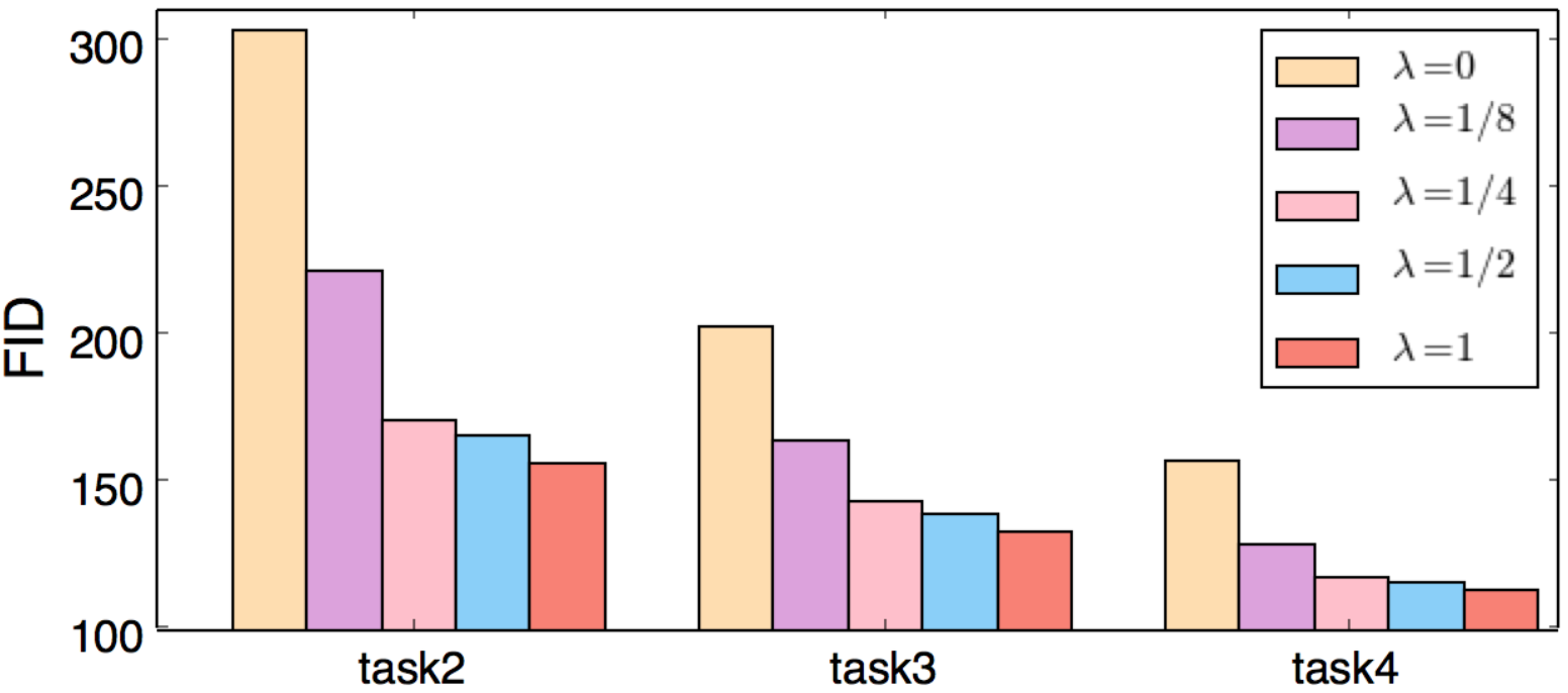
Figure 2: FID for different $\lambda$. Ablation study of choice of different values of $\lambda$. For all upcoming new tasks, the performance improves as $\lambda$ increases. However, while parameter size scales almost linearly with $\lambda$, the improvement of performance slows down gradually.

Ablation study on model components. We also conduct an ablation study on the piggyback filters and unconstrained filters by comparing Piggyback GAN with the baseline models Full, $\frac{1}{4}$Full and Pure Factorization (PF) on Task 2 (maps $\rightarrow$ aerial photos) given the same model trained on Task 1 (semantic labels $\rightarrow$ street photos).

The quantitative evaluations of all approaches are summarized in Table 1. The baseline $\frac{1}{4}$Full produces the worst classification accuracy. Since the details like building blocks are hardly visible, the classifier sometimes mistakes category facades for category maps. The baseline PF generates images that contain more details as compared to the images generated using $\frac{1}{4}$Full. This suggests that piggyback filters can provide valuable information of the patterns in the training data. High FID scores for baselines $\frac{1}{4}$Full and PF indicate that generation qualities for both approaches are poor, and it is observed that the generated images are blurry, resulting in lots of missing details, and also contain lots of artifacts for both approaches. Our Piggyback GAN is parameter efficient and produces images having similar quality as the Full model.

	Full	$\frac{1}{2}$Full	$\frac{1}{4}$Full	PF	Piggyback GAN
Acc	97.90	88.10	84.87	99.82	97.99
FID	156.23	189.08	285.71	303.90	171.04

Table 1: Model components. Ablation study of model components on paired image-conditioned generation tasks. Different models are trained and evaluated on task 2, FID and classification score on task 2 is reported.

Generalization ability. To demonstrate the generalization ability of our model, we learn the same $T_{2}$: maps $\rightarrow$ aerial photos with three different initial tasks $T_{1}$: semantic labels $\rightarrow$ street photos, segmentations $\rightarrow$ facades, and edges $\rightarrow$ handbag photos to evaluate whether Piggyback GAN could generalize well. The quantitative evaluation of all approaches are summarized in Table 2. The experimental results indicate that Piggyback GAN performs stable. The consistent Acc and FID scores indicate that the generated images on task $T_{2}$ from all three initial tasks $T_{1}$ have similar high image quality.

$T_{1}$	semantic labels $\downarrow$ street photos	segmentations $\downarrow$ facades	edges $\downarrow$ handbags
Acc	97.99	97.08	98.09
FID	171.04	174.67	166.20

Table 2: Generalizability. Given different models trained for different initial tasks $T_{1}$, same new task $T_{2}$ is learnt. The consistent Acc and FID scores indicate that our model generalize well and perform consistently well given different set of filter banks achieved from different tasks.

Comparison with SOTA method and baselines. We compare Piggyback GAN with the state-of-the-art approach [24], Sequential Fine-tuning (SFT) and baseline Full. Baseline Full can be considered as the “upper bound” approach, which provides the best performance that Piggyback GAN and [24] could achieve. For both Piggyback GAN and sequential fine-tuning, the model of Task2 is initialized from the same model trained on Task1. The same model also serves as the backbone network for approach [24].

Generated images of each task for all approaches are shown in Figure 3 and the quantitative evaluations of all approaches are summarized in Table 3. It is clear that the sequentially fine-tuned model completely forgets the previous task and can only generate incoherent edges2handbags-like (edges $\rightarrow$ handbag photos)-like patterns. The classification accuracy suggests that state-of-the-art approach [24] is able to adapt to the new task. However, it fails to capture the fine details of the new task, thus resulting in large artifacts in the generated images, especially for task 2 (maps $\rightarrow$ aerial photos) and task 4 (edges $\rightarrow$ handbag photos). In contrast, Piggyback GAN learns the current generative task while remembering the previous task and can better preserve the quality of generated images while shrinking the number of parameters by reusing the filters from previous tasks.

	Piggyback GAN	[24]	SFT	Full
Acc	89.80	88.09	24.92	91.10
FID	137.87	178.16	259.76	130.71

Table 3: Quantitative evaluation among different approaches for continual learning of paired image-conditioned generation tasks. Different models are trained and evaluated on tasks 1-4 based on the same model trained on task 1. The average FID score over 4 tasks is reported.

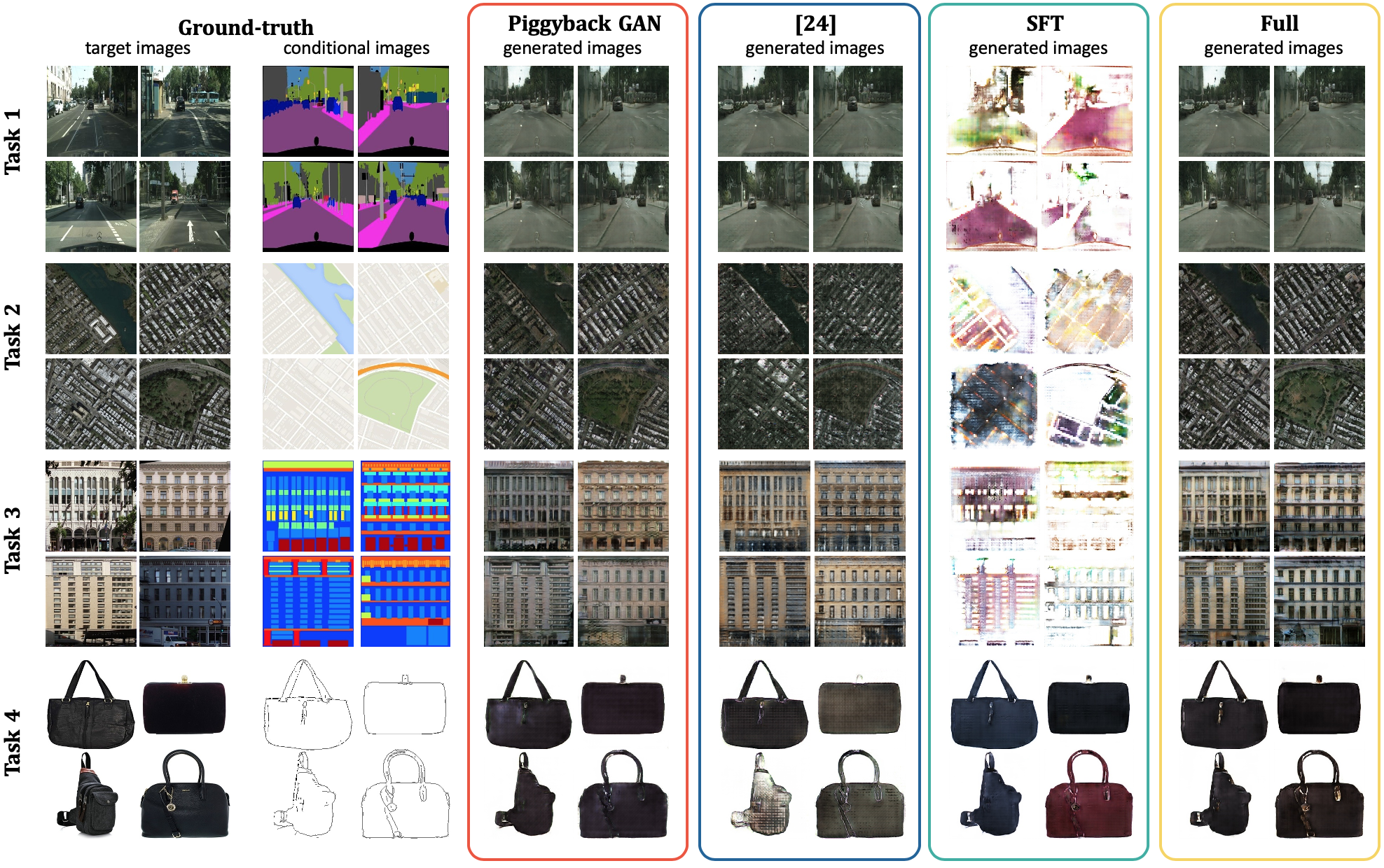
Figure 3: Comparison among different approaches for continual learning of paired image-conditioned generation tasks. Piggyback GAN can learn the current task without forgetting the previous ones, and preserve the generation quality while shrinking the number of parameters by “piggybacking” on an existing model.

For paired image generation, we also compare our approach with Lifelong GAN [42] and Progressive Network (PN) [28]. The FID of PN over all tasks is $141.29$. Lifelong GAN suffers from quality degradation: the FID on cityscapes increases from 122.52 to 160.28 then to 221.07 as tasks are added, while Piggyback GAN ensures no quality degradation since the filters for previous tasks are not altered. These results show the effectiveness and the flexibility of combining the two types of filters of Piggyback GAN.

4.2 Unpaired Image-conditioned Generation

We also apply Piggyback GAN to another challenging scenario: unpaired image-conditioned generation $\mathrm{domain}\,A\rightarrow\mathrm{domain}\,B$. The model is trained on unpaired data, where correspondence between domain $A$ and domain $B$ does not exist, namely for each image in domain $A$ there is no corresponding ground-truth image in domain $B$. We apply our model on 2 sequences of tasks: tasks of image-to-image translation and tasks of style transfer.

Tasks of image-to-image translation. We convert the same 4 tasks from the paired scenario to the unpaired scenario, and compared our approach with Full, the state-of-the-art approach [24] and Sequential Fine-tuning (SFT). The results are shown in Table 4. We observed that the Sequential Fine-tuning (SFT) cannot remember previous tasks and suffers catastrophic forgetting. Our approach produces images with high quality on par with Full model, while [24] is capable of learning each new task, however the generation quality is poor.

Tasks of style transfer. Two tasks in a given sequence may share the same input domain but have different output domains, e.g. $T_{1}$ is Photo $\rightarrow$ Monet Paintings and $T_{2}$ is Photo $\rightarrow$ Ukiyo-e Paintings. While this is not a problem when training each task separately, it does cause problems for lifelong learning. We explore a sequence of tasks of unpaired image-conditioned generation as described above. The first task is unpaired image-to-image translation of photos $\rightarrow$ Monet paintings, the second task is unpaired image-to-image translation of photos $\rightarrow$ Ukiyo-e paintings.

We compare Piggyback GAN against the state-of-the-art approach [24], Sequential Fine-tuning (SFT) and baseline Full which serves as the “upper bound” approach. For both Piggyback GAN and sequential fine-tuning, the model of Task 2 is initialized from the same model trained on Task 1, which also serves as the backbone network for approach [24] to allow for fair comparison.

The quantitative and qualitative evaluations for comparison among different approaches are shown in Table 4 and Figure 4, respectively. The baseline SFT completely forgets the previous Monet style and can only produce images in the Ukiyo-e style. Both the state-of-the-art approach [24] and Piggyback GAN are able to adapt to the new style. The classification accuracy and FID scores indicate that Piggyback GAN can better preserve the quality of generated images, and produce images with styles most closely resembling Ukiyo-e paintings.

Tasks	4 Image-to-image Translation Tasks
Methods	Piggyback GAN	[24]	SFT	Full
Acc	90.30	88.29	24.85	91.04
FID	113.89	149.51	262.37	109.46
Tasks	2 Style Transfer Tasks
Methods	Piggyback GAN	[24]	SFT	Full
Acc	77.97	70.58	50.00	78.97
FID	106.95	118.26	135.05	101.09

Table 4: Unpaired image conditioned generation tasks. Different models are trained on all tasks based on the same model trained on task 1. The average score over all tasks is reported.

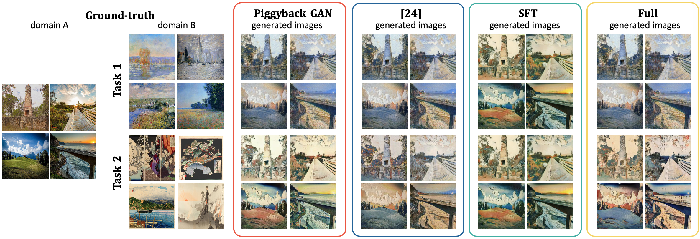
Figure 4: Comparison among different approaches for continual learning of unpaired style transfer tasks. Piggyback GAN can preserve the generation quality the current task most without forgetting the previous ones.

5 Conclusion

We proposed Piggyback GAN for lifelong learning of generative networks, which can handle various conditional generation tasks across different domains. Compared to the naive approach of training a separate standalone model for each task, our approach is parameter efficient since it learns to perform new tasks by making use of the model trained on previous tasks and combining with a small portion of unconstrained filters. At the same time, our model is able to maintain image generation quality comparable to the single standalone model for each task. Since the filters learned for previous tasks are preserved, our model is capable of preserving the exact generation quality of previous tasks. We validated our approach on various image-conditioned generation tasks across different domains, and the qualitative and quantitative results show our model addresses catastrophic forgetting effectively and efficiently.

References

- [1] Abadi, M., Barham, P., Chen, J., Chen, Z., Davis, A., Dean, J., Devin, M., Ghemawat, S., Irving, G., Isard, M., et al.: Tensorflow: A system for large-scale machine learning. In: Symposium on Operating Systems Design and Implementation (OSDI) (2016)
- [2] Aljundi, R., Babiloni, F., Elhoseiny, M., Rohrbach, M., Tuytelaars, T.: Memory aware synapses: Learning what (not) to forget. In: European Conference on Computer Vision (ECCV) (2018)
- [3] Aljundi, R., Chakravarty, P., Tuytelaars, T.: Expert gate: Lifelong learning with a network of experts. In: IEEE Conference on Computer Vision and Pattern Recognition (CVPR) (2017)
- [4] Castro, F.M., Marín-Jiménez, M.J., Guil, N., Schmid, C., Alahari, K.: End-to-end incremental learning. In: European Conference on Computer Vision (ECCV) (2018)
- [5] Chaudhry, A., Dokania, P.K., Ajanthan, T., Torr, P.H.: Riemannian walk for incremental learning: Understanding forgetting and intransigence. In: European Conference on Computer Vision (ECCV) (2018)
- [6] Chaudhry, A., Ranzato, M., Rohrbach, M., Elhoseiny, M.: Efficient lifelong learning with a-gem. In: International Conference on Learning Representations (ICLR) (2019)
- [7] Chen, C., Tung, F., Vedula, N., Mori, G.: Constraint-aware deep neural network compression. In: European Conference on Computer Vision (ECCV) (2018)
- [8] Choi, Y., Choi, M., Kim, M., Ha, J.W., Kim, S., Choo, J.: Stargan: Unified generative adversarial networks for multi-domain image-to-image translation. In: IEEE Conference on Computer Vision and Pattern Recognition (CVPR) (2018)
- [9] Cordts, M., Omran, M., Ramos, S., Rehfeld, T., Enzweiler, M., Benenson, R., Franke, U., Roth, S., Schiele, B.: The cityscapes dataset for semantic urban scene understanding. In: IEEE Conference on Computer Vision and Pattern Recognition (CVPR) (2016)
- [10] Denil, M., Shakibi, B., Dinh, L., Ranzato, M., de Freitas, N.: Predicting parameters in deep learning. In: Advances in Neural Information Processing Systems (NeurIPS) (2013)
- [11] Gatys, L.A., Ecker, A.S., Bethge, M.: Image style transfer using convolutional neural networks. In: IEEE Conference on Computer Vision and Pattern Recognition (CVPR) (2016)
- [12] He, Y., Liu, P., Wang, Z., Hu, Z., Yang, Y.: Filter pruning via geometric median for deep convolutional neural networks acceleration. In: IEEE Conference on Computer Vision and Pattern Recognition (CVPR) (2019)
- [13] Heusel, M., Ramsauer, H., Unterthiner, T., Nessler, B., Hochreiter, S.: Gans trained by a two time-scale update rule converge to a local nash equilibrium. In: Advances in Neural Information Processing Systems (NeurIPS) (2017)
- [14] Isola, P., Zhu, J.Y., Zhou, T., Efros, A.A.: Image-to-image translation with conditional adversarial networks. In: IEEE Conference on Computer Vision and Pattern Recognition (CVPR) (2017)
- [15] Jacob, B., Kligys, S., Chen, B., Zhu, M., Tang, M., Howard, A., Adam, H., Kalenichenko, D.: Quantization and training of neural networks for efficient integer-arithmetic-only inference. In: IEEE Conference on Computer Vision and Pattern Recognition (CVPR) (2018)
- [16] Johnson, J., Alahi, A., Fei-Fei, L.: Perceptual losses for real-time style transfer and super-resolution. In: European Conference on Computer Vision (ECCV) (2016)
- [17] Jung, S., Son, C., Lee, S., Son, J., Han, J.J., Kwak, Y., Hwang, S.J., Choi, C.: Learning to quantize deep networks by optimizing quantization intervals with task loss. In: IEEE Conference on Computer Vision and Pattern Recognition (CVPR) (2019)
- [18] Kingma, D.P., Ba, J.: Adam: A method for stochastic optimization. In: International Conference on Learning Representations (ICLR) (2015)
- [19] Kirkpatrick, J., Pascanu, R., Rabinowitz, N., Veness, J., Desjardins, G., Rusu, A.A., Milan, K., Quan, J., Ramalho, T., Grabska-Barwinska, A., Hassabis, D., Clopath, C., Kumaran, D., Hadsell, R.: Overcoming catastrophic forgetting in neural networks. Proceedings of the National Academy of Sciences of the United States of America (2017)
- [20] Li, Z., Hoiem, D.: Learning without forgetting. IEEE transactions on pattern analysis and machine intelligence 40(12), 2935–2947 (2017)
- [21] Liu, S., Johns, E., Davison, A.J.: End-to-end multi-task learning with attention. In: IEEE Conference on Computer Vision and Pattern Recognition (CVPR) (2019)
- [22] Lopez-Paz, D., Ranzato, M.: Gradient episodic memory for continual learning. In: Advances in Neural Information Processing Systems (NeurIPS) (2017)
- [23] Ma, N., Zhang, X., Zheng, H.T., Sun, J.: Shufflenet v2: Practical guidelines for efficient cnn architecture design. In: European Conference on Computer Vision (ECCV) (2018)
- [24] Mallya, A., Davis, D., Lazebnik, S.: Piggyback: Adapting a single network to multiple tasks by learning to mask weights. In: European Conference on Computer Vision (ECCV) (2018)
- [25] McCloskey, M., Cohen, N.J.: Catastrophic interference in connectionist networks: The sequential learning problem. In: Psychology of Learning and Motivation (1989)
- [26] Qiao, S., Lin, Z., Zhang, J., Yuille, A.: Neural rejuvenation: Improving deep network training by enhancing computational resource utilization. In: IEEE Conference on Computer Vision and Pattern Recognition (CVPR) (2019)
- [27] Rebuffi, S.A., Bilen, H., Vedaldi, A.: Efficient parameterization of multi-domain deep neural networks. In: IEEE Conference on Computer Vision and Pattern Recognition (CVPR) (2018)
- [28] Rusu, A.A., Rabinowitz, N.C., Desjardins, G., Soyer, H., Kirkpatrick, J., Kavukcuoglu, K., Pascanu, R., Hadsell, R.: Progressive neural networks. arXiv:1606.04671 (2016)
- [29] Sandler, M., Howard, A., Zhu, M., Zhmoginov, A., Chen, L.C.: Mobilenetv2: Inverted residuals and linear bottlenecks. In: IEEE Conference on Computer Vision and Pattern Recognition (CVPR) (2018)
- [30] Seff, A., Beatson, A., Suo, D., Liu, H.: Continual learning in generative adversarial nets. In: Advances in Neural Information Processing Systems (NeurIPS) (2017)
- [31] Serrà, J., Suris, D., Miron, M., Karatzoglou, A.: Overcoming catastrophic forgetting with hard attention to the task. In: International Conference on Machine Learning (ICML) (2018)
- [32] Shmelkov, K., Schmid, C., Alahari, K.: Incremental learning of object detectors without catastrophic forgetting. In: IEEE International Conference on Computer Vision (ICCV) (2017)
- [33] Tartaglione, E., Lepsøy, S., Fiandrotti, A., Francini, G.: Learning sparse neural networks via sensitivity-driven regularization. In: Advances in Neural Information Processing Systems (NeurIPS) (2018)
- [34] Tung, F., Mori, G.: Similarity-preserving knowledge distillation. In: IEEE International Conference on Computer Vision (ICCV) (2019)
- [35] Tyleček, R., Šára, R.: Spatial pattern templates for recognition of objects with regular structure. In: German Conference on Pattern Recognition (GCPR) (2013)
- [36] Wu, B., Dai, X., Zhang, P., Wang, Y., Sun, F., Wu, Y., Tian, Y., Vajda, P., Jia, Y., Keutzer, K.: FBNet: Hardware-aware efficient convnet design via differentiable neural architecture search. In: IEEE Conference on Computer Vision and Pattern Recognition (CVPR) (2019)
- [37] Wu, C., Herranz, L., Liu, X., Wang, Y., van de Weijer, J., Raducanu, B.: Memory replay gans: learning to generate images from new categories without forgetting. In: Advances in Neural Information Processing Systems (NeurIPS) (2018)
- [38] Yang, T.J., Howard, A., Chen, B., Zhang, X., Go, A., Sandler, M., Sze, V., Adam, H.: NetAdapt: Platform-aware neural network adaptation for mobile applications. In: European Conference on Computer Vision (ECCV) (2018)
- [39] Yu, A., Grauman, K.: Fine-grained visual comparisons with local learning. In: IEEE Conference on Computer Vision and Pattern Recognition (CVPR) (2014)
- [40] Yu, R., Li, A., Chen, C.F., Lai, J.H., Morariu, V.I., Han, X., Gao, M., Lin, C.Y., Davis, L.S.: NISP: Pruning networks using neuron importance score propagation. In: IEEE Conference on Computer Vision and Pattern Recognition (CVPR) (2018)
- [41] Zagoruyko, S., Komodakis, N.: Paying more attention to attention: Improving the performance of convolutional neural networks via attention transfer. In: International Conference on Learning Representations (ICLR) (2017)
- [42] Zhai, M., Chen, L., Tung, F., He, J., Nawhal, M., Mori, G.: Lifelong gan: Continual learning for conditional image generation. In: IEEE International Conference on Computer Vision (ICCV) (2019)
- [43] Zhang, D., Yang, J., Ye, D., Hua, G.: LQ-Nets: Learned quantization for highly accurate and compact deep neural networks. In: European Conference on Computer Vision (ECCV) (2018)
- [44] Zhu, J.Y., Park, T., Isola, P., Efros, A.A.: Unpaired image-to-image translation using cycle-consistent adversarial networks. In: IEEE International Conference on Computer Vision (ICCV) (2017)