Hermite Polynomial-based Valuation of American Options with General Jump-Diffusion Processes

Abstract

We present a new approximation scheme for the price and exercise policy of American options. The scheme is based on Hermite polynomial expansions of the transition density of the underlying asset dynamics and the early exercise premium representation of the American option price. The advantages of the proposed approach are threefold. First, our approach does not require the transition density and characteristic functions of the underlying asset dynamics to be attainable in closed form. Second, our approach is fast and accurate, while the prices and exercise policy can be jointly produced. Third, our approach has a wide range of applications. We show that the proposed approximations of the price and optimal exercise boundary converge to the true ones. We also provide a numerical method based on a step function to implement our proposed approach. Applications to nonlinear mean-reverting models, double mean-reverting models, Merton’s and Kou’s jump-diffusion models are presented and discussed.

Keywords: Hermite polynomials, American option, early exercise premium, optimal exercise boundary

JEL codes: C22, C41, G12, G13.

1 Introduction

The valuation of American-style options poses a challenge for both academic and industrial professionals. One of the difficulties comes from the fact that such a valuation process relies on the identification of an optimal exercise policy. So far, considerable effort has been put into simple settings where the underlying asset price follows a log-normal process and the interest rate is constant (i.e., the standard model, or the Black-Scholes model). Within this context, Kim (1990) decomposed the American option price into two parts: the corresponding European option price and an Early Exercise Premium (EEP) that captures the gains from exercising the option prior to its maturity. Similar results are provided by Jacka (1991) and Carr et al. (1992). The EEP representation of the American option price has proved extremely useful because it provides a recursive integral equation for the optimal exercise boundary. Solving the integral equations is key to the valuation process: it identifies the optimal exercise policy, providing a parametric formula for the option price. Such an approach, based on the integral equation, is straightforward to implement and shows significant advantages over other numerical procedures such as methods based on binomial lattices, Monte Carlo simulation, and Partial Differential Equations (PDE). See Brodie and Detemple (2004) for a survey of methods on the valuation of American options.

While the valuation of American options in the standard model has been resolved, empirical evidence suggests that the log-normality assumption does not hold in reality. For example, the “volatility smile” phenomenon is a well-known pattern in option pricing practice. To allow for the consistency of models with empirical regularities, non-constant, or even non-deterministic model parameters should be considered. Unfortunately, analytical results in the standard model can not be generalized to models with stochastic parameters in a straightforward manner. Efforts have been made to solve diffusion models with nonconstant parameters. For example, Jacka and Lynn (1992) considered general contingent claims written on diffusion processes. Detemple and Tian (2002) presented an integral equation approach for the valuation of American-style derivatives when the underlying asset price follows a general diffusion process and the interest rate is stochastic. See Rutkowski (1994), and Gukhal (2001) for the valuation of American options for other non-standard models.

All the above-mentioned methods rely on the fact that the transition density of the underlying asset dynamics admits a closed functional form. Such conditions have limited the scope of stochastic processes that can be considered. Furthermore, even when the transition density exists in closed form, the structure may be quite complex, and in turn, the method may be difficult to implement. To overcome these difficulties, this article presents a systematic treatment of the valuation of American options based on Hermite polynomial expansions and the EEP formula. Therefore, our contributions to the literature are threefold.

The first contribution is that our method does not rely on the existence of analytical solutions to the transition density or the characteristic function of the distribution of the underlying asset price. Moreover, there are no requirements for affine structures. We propose using Hermite polynomials to approximate the transition density for a given jump-diffusion model. The Hermite polynomial approximation is based on Ait-Sahalia (2002, 2008), and Yu (2007). This approach gives an explicit sequence of closed-form solutions to the transition density and is shown to converge to the turn density. See Ait-Sahalia (1999), Egorov, Li, and Xu (2003), Ait-Sahalia and Kimmel (2007, 2010), and Xiu (2014) for studies related to this approach.

The second contribution is that, our method is fast and accurate, while the price and exercise policy can be jointly approximated by our approximation scheme. Owing to the inherent nature of the EEP approach, by solving the integral equations with the Hermite polynomial-based approximation to the transition density, we can generate an approximation of the optimal exercise boundary. In turn, we provide a theorem (Theorem 2 in Subsection 2.3) on the convergence of our proposed approximation. When we increase the order of the Hermite polynomial in the approximation of the transition density, the proposed approximations of the price and exercise boundary of American options further improve. We can control the smoothness and accuracy of the exercise boundary by changing the polynomial order in the expansion of the transition density.

Third, our method can be easily extended to jump-diffusion models and multidimensional cases. The extension is straightforward to implement without additional theoretical/modeling complications. Kou (2002) established the analytical solutions for European option pricing in a jump-diffusion model. However, the American option pricing with jump-diffusion processes remains challenging. Gukhal (2001) derived an EEP formula for the value of American options in a jump-diffusion model. Despite all these efforts, one major drawback is that jump-diffusion models usually come without closed-form transition densities. Even if such a density exists, its functional form may be quite complicated in structure and the implementation requires a significant amount of human and computer power. Our method, on the other hand, can overcome these difficulties. By using a Hermite polynomial expansion, we can control the computational cost of the pricing algorithm by specifying the order of the expansion. Moreover, unlike conventional approaches such as the PDE-based method (finite difference, for example), Hermite polynomial expansions can be applied to a vector of stochastic processes, and the results can be directly applied to multi-dimensional models.

The structure of this paper is as follows. Section 2 describes an approach to the American option valuation when the underlying asset prices follow a general diffusion process. Section 3 describes the generalization of the method to jump-diffusion processes. Section 4 presents a numerical algorithm for implementing the proposed approach. Section 5 provides several examples to demonstrate the efficiency of the proposed approach. Finally, Section 6 concludes this paper.

2 Valuation of American Options in Diffusion Models

2.1 American Options

We consider the stock price $S$ defined on a probability space $\left(\varOmega,\mathcal{F},\mathbb{P}^{*}\right)$ with filtration $\mathbb{F}=\left(\mathcal{F}_{t}\right)_{0\leq t\leq T}$ satisfying the usual conditions and following:

$$dS_{t}=\left(r\left(S_{t};\theta\right)-\delta\left(S_{t};\theta\right)\right)dt+\sigma\left(S_{t};\theta\right)dW_{t}.$$ (1)

We also denote $\mu\left(S_{t};\theta\right)=r\left(S_{t};\theta\right)-\delta\left(S_{t};\theta\right)$. Let $D_{S}=\left(\underline{s},\bar{s}\right)$ be the domain of the diffusion $S$.

The arbitrage-free price of an American put option with a finite expiration $T>0$ and a strike price $K$ can be expressed as the expected value of its discounted payoff:

$$P\left(t,S_{t}\right)=\sup_{t\leq\tau\leq T}\mathbb{E}^{*}\left[e^{-\left(\tau-t\right)r}\left(K-S_{\tau}\right)^{+}|S_{t}\right]$$ (2)

under the risk-neutral probability measure $\mathbb{P}^{*}$. Here $\tau$ is the stopping time.

2.2 Early Exercise Boundary

Let $\mathcal{B}=\left\{B_{t}:B_{t}\geq 0,t\in\left[0,T\right]\right\}$ denote the optimal early exercise boundary of the American put option. Then the arbitrage-free price of the American put option, $P\left(t,S_{t}\right)$, solves the following free boundary problem:

$$\mathcal{L}P=0,$$

$$P\left(T,S_{T}\right)=\left(K-S_{T}\right)^{+},$$

$$\lim_{S_{t}\uparrow\infty}P\left(t,S_{t}\right)=0,$$

$$\lim_{S_{t}\downarrow B_{t}}P\left(t,S_{t}\right)=K-B_{t},$$

$$\lim_{S_{t}\downarrow B_{t}}\frac{\partial P\left(t,S_{t}\right)}{\partial S_{t}}=-1,$$

where $\mathcal{L}f=\frac{1}{2}\sigma^{2}S_{t}^{2}\frac{\partial^{2}f}{\partial S_{t}^{2}}+\left(r-\delta\right)S_{t}\frac{\partial f}{\partial S_{t}}-rf+\frac{\partial f}{\partial t}.$

Theorem 1 (Exercise Premium Representation)

We assume that $r$, $\delta$, and $\sigma$ are continuously differentiable, and (1) has a unique strong solution. Then, in the continuation region $\mathcal{C}$, the value of the American put option, $P_{0}\equiv P\left(0,S_{0}=s_{0}\right)$, has the following early exercise premium representation:

$$P_{0}=p_{0}+e_{0}$$ (3)

where $p_{0}$ represents the price of a European put option, that is,

$$p_{0}\equiv p\left(0,S_{0}=s_{0}\right)=\int_{0}^{K}e^{-rT}\left(K-S_{T}\right)\psi\left(S_{T};S_{0}=s_{0}\right)dS_{T},$$ (4)

and $e_{0}$ is the early exercise premium given by

$$e_{0}\equiv e\left(0,S_{0}=s_{0},B\left(\cdot\right)\right)=\int_{0}^{T}\int_{0}^{B_{t}}\left(rK-\delta S_{t}\right)e^{-rt}\psi\left(S_{t};S_{0}=s_{0}\right)dS_{t}dt,$$ (5)

and $\psi\left(S_{t};S_{0}=s_{0}\right)$ denotes the risk-neutral transitional density function of $S_{t}$, given $S_{0}=s_{0}$. The exercise boundary $B_{t}$ solves the recursive nonlinear integral equation

$$K-B_{t}=p\left(t,B_{t}\right)+e\left(t,B_{t},B\left(\cdot\right)\right)\quad\forall t\in\left[0,T\right),$$ (6)

subject to the boundary condition

$$B_{T-}\equiv\lim_{t\uparrow T}B_{t}=\min\left\{K,\frac{r\left(B_{T};\theta\right)}{\delta\left(B_{T};\theta\right)}K\right\}.$$

At maturity, $B_{T}=K\geq B_{T-}$. The functions $p$ and $e$ in (6) are defined as following:

$$p\left(t,B_{t}\right)\equiv\int_{0}^{K}\left(K-S_{T}\right)\psi\left(S_{T};S_{t}=B_{t}\right)dS_{T},$$ (7)

$$e\left(t,B_{t},B\left(\cdot\right)\right)\equiv\int_{t}^{T}\int_{0}^{B_{s}}\left(rK-\delta S_{s}\right)e^{-r\left(s-t\right)}\psi\left(S_{s};S_{t}=B_{t}\right)dS_{s}ds.$$ (8)

The equations (4)-(6) in Theorem 1 for the valuation of American options can be simplified if we make further assumptions on the model. For example, if we assume that the stock price follows a geometric Brownian Motion (GBM), that is, $r\left(S_{t};\theta\right)=r$, $\sigma\left(S_{t};\theta\right)=\sigma$ for constants $r$ and $\sigma$, and $\delta\left(S_{t};\theta\right)=0$, then we have a Black-Scholes style formula for the valuation of American options. We summarize this result in the following lemma.

Lemma 1 (Exercise Premium Representation under GBM)

If the stock price $S$ follows geometric Brownian Motion, then the value of the American put option, $P_{0}$, can be written as:

$$P_{0}=Ke^{-rT}N\left(k_{2}\left(S_{0},K,T\right)\right)-S_{0}N\left(k_{1}\left(S_{0},K,T\right)\right)+rk\int_{0}^{T}e^{-rt}N\left(b_{2}\left(S_{0},B_{t},t\right)\right)dt,$$ (9)

where

$$k_{1}\left(S_{0},K,T\right)\equiv\frac{\log\left(K/S_{0}\right)-\rho_{1}T}{\sigma\sqrt{T}},$$

$$k_{2}\left(S_{0},K,T\right)\equiv\frac{\log\left(K/S_{0}\right)-\rho_{2}T}{\sigma\sqrt{T}},$$

$$\rho_{1}\equiv\rho_{2}+\sigma^{2}=r+\frac{\sigma^{2}}{2},$$

$$b_{2}\left(S_{0},B_{t},t\right)\equiv\frac{\log\left(B_{t}/S_{0}\right)-\rho_{2}t}{\sigma\sqrt{t}},$$

and $B_{t}$ solves the following integral equation:

$$K-B_{t}=Ke^{-r\left(T-t\right)}N\left(k_{2}\left(B_{t},K,T-t\right)\right)-B_{t}N\left(k_{1}\left(B_{t},K,T-t\right)\right)\\ +rk\int_{t}^{T}e^{-r\left(s-t\right)}N\left(b_{2}\left(B_{t},B_{s},s-t\right)\right)ds.$$ (10)

2.3 Hermite Polynomial-based Approximation

Theorem 1 provides an intuitive approach to the valuation of American options in diffusion models; however, we still have two difficulties. First, most of the diffusion models do not admit a closed-form solution for the transition density. Second, the exercise boundary $\mathcal{B}$ is unknown in (5), and we need to solve the integral equation (6) recursively to compute $\mathcal{B}$.

In this study, we propose the use of the Hermite polynomials to approximate the transition density. Our approach is based on the work of Ait-Sahalia (2002, 2006) and Yu (2007). The Hermite polynomial approach by Ait-Sahalia (2002) provided an explicit sequence of closed-form functions to approximate the unknown transition density. Ait-Sahalia (2006) and Yu (2007) extended the approach to multivariate case and jump-diffusion models.

To approximate the transition density of the stock price $S$, we first transform $S$ into a new random variable $Y$ by defining $Y\equiv\gamma\left(S\right)=\int^{S}du/\sigma\left(u\right)$. We know that $Y$ has a unit diffusion, that is,

$$dY_{t}=\mu_{Y}\left(Y_{t};\theta\right)dt+dW_{t},$$

where

$$\mu_{Y}\left(y;\theta\right)=\frac{\mu\left(\gamma^{-1}\left(y;\theta\right);\theta\right)}{\sigma\left(\gamma^{-1}\left(y;\theta\right);\theta\right)}-\frac{1}{2}\frac{\partial\sigma}{\partial S}\left(\gamma^{-1}\left(y;\theta\right);\theta\right).$$ (11)

We denote the domain of $Y$ as $D_{Y}=\left(\underline{y},\bar{y}\right)$. According to Ait-Sahalia (2002), the transition density of $Y$ can be approximated using Hermite polynomials, and the transition density of $S$ can then be derived from that of $Y.$ More specifically, the transition density of $S$ with time interval $\varDelta$ can be approximated up to order $m$ as following:

$$\widetilde{\psi}^{\left(m\right)}\left(S_{t+\varDelta}=S^{\prime};S_{t}=S\right)=\sigma^{-1}\left(S^{\prime};\theta\right)\varDelta^{-\frac{1}{2}}\phi\left(\frac{\gamma\left(S^{\prime};\theta\right)-\gamma\left(S;\theta\right)}{\varDelta^{\frac{1}{2}}}\right)\times\\ \exp\left(\int_{\gamma\left(S;\theta\right)}^{\gamma\left(S^{\prime};\theta\right)}\mu\left(w;\theta\right)dw\right)\times\sum_{k=0}^{m}c_{k}\left(\gamma\left(S^{\prime};\theta\right)|\gamma\left(S;\theta\right);\theta\right)\frac{\varDelta^{k}}{k!},$$ (12)

where $\phi\left(z\right)\equiv\exp\left(-z^{2}/2\right)/\sqrt{2\pi}$ denotes the density function of standard normal distribution, and for all $j\geq 1$,

$$c_{j}\left(\gamma\left(S^{\prime};\theta\right)|\gamma\left(S;\theta\right);\theta\right)=j\left(S^{\prime}-S\right)^{-j}\int_{\gamma\left(S;\theta\right)}^{\gamma\left(S^{\prime};\theta\right)}\left(w-\gamma\left(S;\theta\right)\right)^{j-1}\\ \times\left\{\lambda\left(w;\theta\right)c_{j-1}\left(w|\gamma\left(S;\theta\right);\theta\right)+\left(\partial^{2}c_{j-1}\left(w|\gamma\left(S;\theta\right);\theta\right)/\partial w^{2}\right)/2\right\}dw$$ (13)

where $\lambda\left(x;\theta\right)\equiv-\left(\mu_{Y}^{2}\left(x;\theta\right)+\partial\mu_{Y}\left(x;\theta\right)/\partial x\right)/2$ with $\mu_{Y}$ defined in (11), and $c_{0}=1.$

Once we obtain the approximation of the transition density of $S$ in (12), we can plug $\widetilde{\psi}^{\left(m\right)}$ into Theorem 1 and obtain the approximation of the valuation of American options. More specifically, we have the following approximated early exercise premium representation for the value of the American put option up to order $m$:

$$\widetilde{P}_{0}^{\left(m\right)}=\widetilde{p}_{0}^{\left(m\right)}+\widetilde{e}_{0}^{\left(m\right)}$$ (14)

where $\widetilde{p}_{0}^{\left(m\right)}\equiv\widetilde{p}^{\left(m\right)}\left(0,S_{0}=s_{0}\right)=\int_{0}^{K}e^{-rT}\left(K-S_{T}\right)\widetilde{\psi}^{\left(m\right)}\left(S_{T};S_{0}=s_{0}\right)dS_{T}$ represents the approximated price of a European put option and $\widetilde{e}_{0}^{\left(m\right)}$ is the approximated early exercise premium given by

$$\widetilde{e}_{0}^{\left(m\right)}\equiv\widetilde{e}^{\left(m\right)}\left(0,S_{0}=s_{0},\widetilde{B}^{\left(m\right)}\left(\cdot\right)\right)=\int_{0}^{T}\int_{0}^{\widetilde{B}_{t}^{\left(m\right)}}\left(rK-\delta S_{t}\right)e^{-rt}\widetilde{\psi}^{\left(m\right)}\left(S_{t};S_{0}=s_{0}\right)dS_{t}dt.$$ (15)

The approximated exercise boundary up to order $m$, $\widetilde{B}_{t}^{\left(m\right)}$, solves the following recursive nonlinear integral equation:

$$K-\widetilde{B}_{t}^{\left(m\right)}=\widetilde{p}^{\left(m\right)}\left(t,\widetilde{B}_{t}^{\left(m\right)}\right)+\widetilde{e}^{\left(m\right)}\left(t,\widetilde{B}_{t}^{\left(m\right)},\widetilde{B}^{\left(m\right)}\left(\cdot\right)\right)\quad\forall t\in\left[0,T\right).$$ (16)

Similarly to (7)–(8), $\widetilde{p}^{\left(m\right)}$ and $\widetilde{e}^{\left(m\right)}$ are defined as:

$$\widetilde{p}^{\left(m\right)}\left(t,\widetilde{B}_{t}^{\left(m\right)}\right)\equiv\int_{0}^{K}\left(K-S_{T}\right)\widetilde{\psi}^{\left(m\right)}\left(S_{T};S_{t}=\widetilde{B}_{t}^{\left(m\right)}\right)dS_{T},$$ (17)

$$\widetilde{e}^{\left(m\right)}\left(t,\widetilde{B}_{t}^{\left(m\right)},\widetilde{B}^{\left(m\right)}\left(\cdot\right)\right)\equiv\int_{t}^{T}\int_{0}^{\widetilde{B}_{s}^{\left(m\right)}}\left(rK-\delta S_{s}\right)e^{-r\left(s-t\right)}\widetilde{\psi}^{\left(m\right)}\left(S_{s};S_{t}=\widetilde{B}_{t}^{\left(m\right)}\right)dS_{s}ds,$$ (18)

subject to the boundary condition

$$\widetilde{B}_{T-}^{\left(m\right)}\equiv\lim_{t\uparrow T}\widetilde{B}_{t}^{\left(m\right)}=\min\left\{K,\frac{r\left(B_{T};\theta\right)}{\delta\left(B_{T};\theta\right)}K\right\},$$

and $\widetilde{B}_{T}^{\left(m\right)}=B_{T}=K\geq\widetilde{B}_{T-}^{\left(m\right)}$.

The following theorem guarantees that the proposed approach in (14)–(18) is a well-behaved approximation of the value of American options.

Theorem 2

Under Assumptions 1–3 given in Appendix A, as $m\rightarrow\infty,$ we have

1. $\widetilde{p}_{0}^{\left(m\right)}\rightarrow p_{0}$,

2. $\widetilde{B}_{t}^{\left(m\right)}\rightarrow B_{t}$ for any $t\in\left[0,T\right]$,

3. $\widetilde{e}_{0}^{\left(m\right)}\rightarrow e_{0}$,

4. $\widetilde{P}_{0}^{\left(m\right)}\rightarrow P_{0}$.

Proof. In Appendix B   

3 Valuation of American Options in Jump-Diffusion Models

3.1 Valuation of American Options

In this section, we discuss the approximation of the value of American options when the underlying asset price follows a jump-diffusion process. Because of the discontinuous nature of the asset price path, the exercise premium representation is different from that without jumps. Specifically, we consider the stock price under the risk-neutral measure, and assume that it follows:

$$d\log S_{t}=\left(r\left(S_{t};\theta\right)-\delta\left(S_{t};\theta\right)-\rho j\right)dt+\sigma\left(S_{t};\theta\right)dW_{t}+\left(J-1\right)dq_{t}$$ (19)

where $dq$ is a Poisson process with rate $\rho t$, $J-1$ is the proportional change in the price due to a jump with density function $\nu$ as a function of jump size with support $D_{J}$, and $j=E\left(J-1\right)$. We assume $r\left(S_{t};\theta\right)$, $\delta\left(S_{t};\theta\right)$, and $\sigma\left(S_{t};\theta\right)$ are smooth functions of $S_{t}$. Then, based on Gukhal (2001), the value of the American put option, $P_{0}\equiv P\left(0,S_{0}=s_{0}\right)$, has the following representation:

$$P_{0}=p_{0}+e_{0}+g_{0}$$ (20)

where

$$p_{0}\equiv p\left(0,S_{0}=s_{0}\right)=\int_{0}^{K}e^{-rT}\left(K-S_{T}\right)\psi\left(S_{T};S_{0}=s_{0}\right)dS_{T}$$ (21)

$$e_{0}\equiv e\left(0,S_{0}=s_{0},B\left(\cdot\right)\right)=\int_{0}^{T}\int_{0}^{B_{t}}\left(rK-\delta S_{t}\right)e^{-rt}\psi\left(S_{t};S_{0}=s_{0}\right)dS_{t}dt$$ (22)

and

$$g_{0}\equiv g\left(0,S_{0}=s_{0},B\left(\cdot\right)\right)=\int_{0}^{T}\int_{0}^{B_{t-}}\int_{B_{t}}^{\infty}e^{-rt}\rho\left(P\left(t,J_{t}S_{t-}\right)-\left(K-J_{t}S_{t-}\right)\right)\\ \times\psi\left(S_{t-};S_{0}=s_{0}\right)\psi\left(J_{t}S_{t-};S_{t-}\right)d\left(J_{t}S_{t-}\right)dS_{t-}dt.$$ (23)

The exercise boundary $B_{t}$ solves the following integral equation

$$K-B_{t}=p\left(t,B_{t}\right)+e\left(t,B_{t},B\left(\cdot\right)\right)-g\left(t,B_{t},B\left(\cdot\right)\right)$$ (24)

where

$$p\left(t,B_{t}\right)=\int_{0}^{K}\left(K-S_{T}\right)\psi\left(S_{T};B_{t}\right)dS_{T}$$

$$e\left(t,B_{t},B\left(\cdot\right)\right)=\int_{t}^{T}\int_{0}^{B_{s}}\left(rK-\delta S_{s}\right)e^{-r\left(s-t\right)}\psi\left(S_{s};B_{t}\right)dS_{s}ds$$

$$g\left(t,B_{t},B\left(\cdot\right)\right)=\int_{t}^{T}\int_{0}^{B_{s-}}\int_{B_{s}}^{\infty}e^{-r\left(s-t\right)}\rho\left(P\left(s,J_{s}S_{s-}\right)-\left(K-J_{s}S_{s-}\right)\right)\\ \times\psi\left(S_{s-};B_{t}\right)\psi\left(J_{s}S_{s-};S_{s-}\right)d\left(J_{s}S_{s-}\right)dS_{s-}ds.$$

The representation in (20) has a straightforward interpretation. As in the case without jumps, $p_{0}$ represents the price of a European put option, $e_{0}$ is the early exercise premium, and $g_{0}$ is the rebalancing cost due to the jumps of stock prices from the exercise region (the stock price is below the exercise boundary) into the continuation region (the stock price is above the exercise boundary).

3.2 Hermite Polynomial-based Approximation

Our approach to studying jump-diffusion models is similar to our approach in Section 2. We first approximate the transition density using Hermite polynomials. According to Yu (2007), an approximation of the order $m>0$ is obtained as follows:

$$\widetilde{\psi}^{\left(m\right)}\left(S_{t+\varDelta}=S^{\prime};S_{t}=S\right)=\varDelta^{-\frac{1}{2}}\exp\left[-\frac{C^{\left(-1\right)}\left(S,S^{\prime}\right)}{\varDelta}\right]\sum_{k=0}^{m}C^{\left(k\right)}\left(S,S^{\prime}\right)\varDelta^{k}\\ +\sum_{k=1}^{m}D^{\left(k\right)}\left(S,S^{\prime}\right)\varDelta^{k}$$ (25)

where

$$C^{\left(-1\right)}\left(S,S^{\prime}\right)=\frac{1}{2}\left[\int_{S}^{S^{\prime}}\sigma\left(s\right)^{-1}ds\right]^{2},$$ (26)

$$C^{\left(0\right)}\left(S,S^{\prime}\right)=\frac{1}{\sqrt{2\pi}\sigma\left(S^{\prime}\right)}\exp\left[\int_{S}^{S^{\prime}}\frac{\mu\left(s\right)}{\sigma^{2}\left(s\right)}-\frac{\sigma^{\prime}\left(s\right)}{2\sigma\left(s\right)}ds\right],$$ (27)

$$C^{\left(k+1\right)}\left(S,S^{\prime}\right)=-\left[\int_{S}^{S^{\prime}}\sigma\left(s\right)^{-1}ds\right]^{-k+1}\int_{S}^{S^{\prime}}\left\{\exp\left[\int_{u}^{S}\frac{\mu\left(u\right)}{\sigma^{2}\left(u\right)}-\frac{\sigma^{\prime}\left(u\right)}{2\sigma\left(u\right)}du\right]\right.\\ \left.\times\sigma\left(s\right)^{-1}\left[\int_{s}^{S^{\prime}}\sigma\left(u\right)^{-1}du\right]^{k}\left[\rho\left(s\right)-\mathcal{L}\right]C^{\left(k\right)}\left(s,S^{\prime}\right)\right\}ds,\quad for\;k\geq 0,$$ (28)

$$D^{\left(1\right)}\left(S,S^{\prime}\right)=\rho\left(S\right)-\upsilon\left(S^{\prime}-S\right),$$ (29)

$$D^{\left(k+1\right)}\left(S,S^{\prime}\right)=\frac{1}{1+k}\left[\mathfrak{L}D^{\left(k\right)}\left(S,S^{\prime}\right)+\right.\\ \left.\sqrt{2\pi}\rho\left(S\right)\sum_{r=0}^{k}\frac{M_{2r}^{1}}{\left(2r\right)!}\frac{\partial^{2r}}{\partial w^{2r}}m_{k-r}\left(S,S^{\prime},w\right)|_{w=0}\right],\quad for\;k\geq 0,$$ (30)

where

$$m_{k}\left(S,S^{\prime},w\right)\equiv C^{\left(k\right)}\left(w_{B}^{-1}\left(w\right),S^{\prime}\right)\upsilon\left(w_{B}^{-1}\left(w\right)-S\right)\sigma\left(w_{B}^{-1}\left(w\right)\right),$$ (31)

$$M_{2r}^{1}\equiv 1/\sqrt{2\pi}\int_{\mathbb{R}}\exp\left(-s^{2}/2\right)s^{2r}ds,$$ (32)

$$w_{B}\left(S,S^{\prime}\right)=\int_{S^{\prime}}^{S}\sigma\left(s\right)^{-1}ds,$$ (33)

$$\mathscr{L}f\left(s,s^{\prime}\right)=\frac{1}{2}\sigma^{2}s^{2}\frac{\partial^{2}f}{\partial s^{2}}\left(s,s^{\prime}\right)+\left(r-\delta-\rho j\right)s\frac{\partial f}{\partial s}\left(s,s^{\prime}\right),$$ (34)

and

$$\mathfrak{L}f\left(s,s^{\prime}\right)=\mathscr{L}f\left(s,s^{\prime}\right)+\rho\int_{D_{J}}\left[f\left(s+c,s^{\prime}\right)-f\left(s,s^{\prime}\right)\right]\upsilon\left(c\right)dc.$$ (35)

Once we obtain the Hermite polynomial approximation of the transition density as above, we plug the approximation into (21)-(23), and solve the integral equation (24) recursively. More specifically, we have the approximated value of the American put option up to order $m$, $\widetilde{P}_{0}^{\left(m\right)}\equiv\widetilde{P}^{\left(m\right)}\left(0,S_{0}=s_{0}\right)$:

$$\widetilde{P}_{0}^{\left(m\right)}=\widetilde{p}_{0}^{\left(m\right)}+\widetilde{e}_{0}^{\left(m\right)}+\widetilde{g}_{0}^{\left(m\right)}$$ (36)

where

$$\widetilde{p}_{0}^{\left(m\right)}\equiv\widetilde{p}^{\left(m\right)}\left(0,S_{0}=s_{0}\right)=\int_{0}^{K}e^{-rT}\left(K-S_{T}\right)\widetilde{\psi}^{\left(m\right)}\left(S_{T};S_{0}=s_{0}\right)dS_{T},$$ (37)

$$\widetilde{e}_{0}^{\left(m\right)}\equiv\widetilde{e}^{\left(m\right)}\left(0,S_{0}=s_{0},\widetilde{B}^{\left(m\right)}\left(\cdot\right)\right)=\int_{0}^{T}\int_{0}^{\widetilde{B}_{t}^{\left(m\right)}}\left(rK-\delta S_{t}\right)e^{-rt}\widetilde{\psi}^{\left(m\right)}\left(S_{t};S_{0}=s_{0}\right)dS_{t}dt,$$ (38)

and

$$\widetilde{g}_{0}^{\left(m\right)}\equiv\widetilde{g}^{\left(m\right)}\left(0,S_{0}=s_{0},\widetilde{B}^{\left(m\right)}\left(\cdot\right)\right)=\int_{0}^{T}\int_{0}^{\widetilde{B}_{t-}^{\left(m\right)}}\int_{\widetilde{B}_{t}^{\left(m\right)}}^{\infty}e^{-rt}\rho\left(\widetilde{P}^{\left(m\right)}\left(t,J_{t}S_{t-}\right)-\left(K-J_{t}S_{t-}\right)\right)\\ \times\widetilde{\psi}^{\left(m\right)}\left(S_{t-};S_{0}=s_{0}\right)\widetilde{\psi}^{\left(m\right)}\left(J_{t}S_{t-};S_{t-}\right)d\left(J_{t}S_{t-}\right)dS_{t-}dt.$$ (39)

The approximated exercise boundary up to order $m$, $\widetilde{B}_{t}^{\left(m\right)}$, solves the following recursive nonlinear integral equation:

$$K-\widetilde{B}_{t}^{\left(m\right)}=\widetilde{p}^{\left(m\right)}\left(t,\widetilde{B}_{t}^{\left(m\right)}\right)+\widetilde{e}^{\left(m\right)}\left(t,\widetilde{B}_{t}^{\left(m\right)},\widetilde{B}^{\left(m\right)}\left(\cdot\right)\right)-\widetilde{g}^{\left(m\right)}\left(t,\widetilde{B}_{t}^{\left(m\right)},\widetilde{B}^{\left(m\right)}\left(\cdot\right)\right),$$ (40)

where

$$\widetilde{p}^{\left(m\right)}\left(t,\widetilde{B}_{t}^{\left(m\right)}\right)\equiv\int_{0}^{K}\left(K-S_{T}\right)\widetilde{\psi}^{\left(m\right)}\left(S_{T};S_{t}=\widetilde{B}_{t}^{\left(m\right)}\right)dS_{T},$$ (41)

$$\widetilde{e}^{\left(m\right)}\left(t,\widetilde{B}_{t}^{\left(m\right)},\widetilde{B}^{\left(m\right)}\left(\cdot\right)\right)\equiv\int_{t}^{T}\int_{0}^{\widetilde{B}_{s}^{\left(m\right)}}\left(rK-\delta S_{s}\right)e^{-r\left(s-t\right)}\widetilde{\psi}^{\left(m\right)}\left(S_{s};S_{t}=\widetilde{B}_{t}^{\left(m\right)}\right)dS_{s}ds,$$ (42)

$$\widetilde{g}^{\left(m\right)}\left(t,\widetilde{B}_{t}^{\left(m\right)},\widetilde{B}^{\left(m\right)}\left(\cdot\right)\right)\equiv\int_{t}^{T}\int_{0}^{\widetilde{B}_{s-}^{\left(m\right)}}\int_{\widetilde{B}_{s}^{\left(m\right)}}^{\infty}e^{-r\left(s-t\right)}\rho\left(\widetilde{P}^{\left(m\right)}\left(s,J_{s}S_{s-}\right)-\left(K-J_{s}S_{s-}\right)\right)\\ \times\widetilde{\psi}^{\left(m\right)}\left(S_{s-};\widetilde{B}_{t}^{\left(m\right)}\right)\widetilde{\psi}^{\left(m\right)}\left(J_{s}S_{s-};S_{s-}\right)d\left(J_{s}S_{s-}\right)dS_{s-}ds.$$ (43)

4 Numerical Method and Algorithm

Following Detemple (2006), we divide the period $\left[0,T\right]$ into $N$ equal subintervals and let $\Delta=T/N$. We then use a step function to compute the exercise boundary recursively. The algorithm works as follows: suppose that our step function approximation of the exercise boundary is $\left\{\widetilde{B}_{n\Delta}^{\left(m,N\right)},n=0,\ldots,N\right\}$. The terminal condition tells us that

$$\widetilde{B}_{N\Delta}^{\left(m,N\right)}=\min\left\{K,\frac{r\left(B_{T};\theta\right)}{\delta\left(B_{T};\theta\right)}\times K\right\}.$$

Suppose that $\widetilde{B}_{l\Delta}^{\left(m,N\right)}$ is known for all $l>n$, then $\left\{\widetilde{B}_{l\Delta}^{\left(m,N\right)},l=0,\ldots,n\right\}$ can be obtained by discretizing the integral in (16) for a diffusion model, or (40) for a jump-diffusion model using the trapezoidal rule. For example, we obtain the following equation for diffusion models:

$$K-\widetilde{B}_{l\Delta}^{\left(m,N\right)}=\widetilde{p}^{\left(m\right)}\left(l\Delta,\widetilde{B}_{l\Delta}^{\left(m,N\right)}\right)+\sum_{q=l+1}^{N-l}\widetilde{\epsilon}^{\left(m\right)}\left(\left(q-l\right)\Delta,\widetilde{B}_{l\Delta}^{\left(m,N\right)},\widetilde{B}_{q\Delta}^{\left(m,N\right)}\right)\Delta\\ +\left[\widetilde{\epsilon}^{\left(m\right)}\left(0,\widetilde{B}_{l\Delta}^{\left(m,N\right)},\widetilde{B}_{l\Delta}^{\left(m,N\right)}\right)+\widetilde{\epsilon}^{\left(m\right)}\left(\left(N-l\right)\Delta,\widetilde{B}_{l\Delta}^{\left(m,N\right)},\widetilde{B}_{N\Delta}^{\left(m,N\right)}\right)\right]\frac{\Delta}{2}$$ (44)

where

$$\widetilde{\epsilon}^{\left(m\right)}\left(s\Delta,\widetilde{B}_{t}^{\left(m\right)},\widetilde{B}_{t+s\Delta}^{\left(m\right)}\right)\equiv\int_{0}^{\widetilde{B}_{t+s\Delta}^{\left(m\right)}}\left(rK-\delta S_{t+s\Delta}\right)e^{-rs\Delta}\widetilde{\psi}^{\left(m\right)}\left(S_{t+s\Delta};S_{t}=\widetilde{B}_{t}^{\left(m\right)}\right)dS_{t+s\Delta}$$ (45)

And for jump-diffusion models, we have

$$K-\widetilde{B}_{l\Delta}^{\left(m,N\right)}=\widetilde{p}^{\left(m\right)}\left(l\Delta,\widetilde{B}_{l\Delta}^{\left(m,N\right)}\right)+\sum_{q=l+1}^{N-l}\widetilde{\epsilon}^{\left(m\right)}\left(\left(q-l\right)\Delta,\widetilde{B}_{l\Delta}^{\left(m,N\right)},\widetilde{B}_{q\Delta}^{\left(m,N\right)}\right)\Delta\\ +\left[\widetilde{\epsilon}^{\left(m\right)}\left(0,\widetilde{B}_{l\Delta}^{\left(m,N\right)},\widetilde{B}_{l\Delta}^{\left(m,N\right)}\right)+\widetilde{\epsilon}^{\left(m\right)}\left(\left(N-l\right)\Delta,\widetilde{B}_{l\Delta}^{\left(m,N\right)},\widetilde{B}_{N\Delta}^{\left(m,N\right)}\right)\right]\frac{\Delta}{2}\\ +\left[\widetilde{\eta}^{\left(m\right)}\left(0,\widetilde{B}_{l\Delta}^{\left(m,N\right)},\widetilde{B}_{l\Delta}^{\left(m,N\right)}\right)+\widetilde{\eta}^{\left(m\right)}\left(\left(N-l\right)\Delta,\widetilde{B}_{l\Delta}^{\left(m,N\right)},\widetilde{B}_{N\Delta}^{\left(m,N\right)}\right)\right]\frac{\Delta}{2}\\ +\sum_{q=l+1}^{N-l}\widetilde{\eta}^{\left(m\right)}\left(\left(q-l\right)\Delta,\widetilde{B}_{l\Delta}^{\left(m,N\right)},\widetilde{B}_{q\Delta}^{\left(m,N\right)}\right)\Delta$$ (46)

where $\widetilde{\epsilon}^{\left(m\right)}$ is defined as in (45), and $\widetilde{\eta}^{\left(m\right)}$ is defined by

$$\widetilde{\eta}^{\left(m\right)}\left(s\Delta,\widetilde{B}_{t}^{\left(m\right)},\widetilde{B}_{t+s\Delta}^{\left(m\right)}\right)\equiv\\ \int_{0}^{\widetilde{B}_{t+s\Delta-}^{\left(m\right)}}\int_{\widetilde{B}_{t+s\Delta}^{\left(m\right)}}^{\infty}e^{-rs\Delta}\rho\left(\widetilde{P}^{\left(m\right)}\left(s\Delta,J_{t+s\Delta}S_{t+s\Delta s-}\right)-\left(K-J_{t+s\Delta}S_{t+s\Delta s-}\right)\right)\\ \times\widetilde{\psi}^{\left(m\right)}\left(S_{t+s\Delta-};\widetilde{B}_{t}^{\left(m\right)}\right)\widetilde{\psi}^{\left(m\right)}\left(J_{t+s\Delta}S_{t+s\Delta-};S_{t+s\Delta-}\right)d\left(J_{t+s\Delta}S_{t+s\Delta-}\right)dS_{t+s\Delta-}$$ (47)

We run the above procedure recursively, and obtain the exercise boundary $\left\{\widetilde{B}_{n\Delta}^{\left(m,N\right)},n=0,\ldots,N\right\}$. Finally, the value of the American put option can be computed by substituting the exercise boundary into (14) for diffusion models or (36) for jump-diffusion models.

5 Applications

In this section, we illustrate how to compute the value of the American put option and the corresponding exercise boundary for diffusion models and jump-diffusion models. We use these examples to illustrate the accuracy and speed of the proposed approach. We approximate the transition density using $m=2$ for all the examples in this section.

5.1 Applications to Diffusion Models

5.1.1 Geometric Brownian Motion (GBM) Model

In the geometric Brownian Motion model, the stock price $S$ follows

$$dS_{t}=\left(r-\delta\right)S_{t}dt+\sigma S_{t}dW_{t},$$

where $r$, $\delta$, and $\sigma$ are constants. To test the efficiency of our recursive algorithm in Section 2, we compare the results from our approach with those from four widely used methods: the binomial method by Cox, Ross, and Rubinstein (1979), the accelerated binomial methods by Breen (1991), the finite difference method, and the analytical approximation by Geske and Johnson (1984). We use the results from the binomial method with 10,000 time-steps as a benchmark to measure the accuracy. Following Huang et al. (1996) and Geske and Johnson (1984), we set $S_{0}=40$, $r=4.88\%$, and $\delta=0$.

Table 1 reports the valuations of American options from the six approaches. Columns 1 through 3 represent the values of the parameters, $K$ (strike price), $\sigma$ (volatility), and $T$ (maturity), respectively. Column 4 gives the numerical results from the binomial method with 10,000 time-steps, and we take this approach as a benchmark. Column 5 includes the results in Table I of Geske and Johnson (1984). Columns 6 through 8 report the results from the binomial method with 150 time-steps, the finite difference method with 200 steps, and the accelerated binomial method with 150 time-steps. Column 9 shows the results of the proposed approach with 100 time-steps. The accuracy is measured by the root mean squared error, as shown in the last row. It is clear from this table that the proposed approach achieves the best performance in terms of accuracy compared with the other methods.

Table 1: Value of American Options Based on Different Numerical Methods

K	$\sigma$	T (yr)	Binomial	G&J	Binomial II	Accelerated	FD	Hermite
35	0.2	0.0833	0.0062	0.0062	0.0061	0.0061	0.0278	0.0062
35	0.2	0.3333	0.2004	0.1999	0.1995	0.1994	0.2382	0.2004
35	0.2	0.5833	0.4328	0.4321	0.4340	0.4331	0.4624	0.4329
40	0.2	0.0833	0.8522	0.8528	0.8512	0.8517	0.9874	0.8523
40	0.2	0.3333	1.5798	1.5807	1.5783	1.5752	1.6244	1.5800
40	0.2	0.5833	1.9904	1.9905	1.9886	1.9856	2.0177	1.9906
45	0.2	0.0833	5.0000	4.9985	5.0000	4.9200	5.0052	5.0000
45	0.2	0.3333	5.0883	5.0951	5.0886	4.9253	5.1327	5.0886
45	0.2	0.5833	5.2670	5.2719	5.2677	5.2844	5.2699	5.2673
35	0.3	0.0833	0.0774	0.0744	0.0775	0.0772	0.1216	0.0774
35	0.3	0.3333	0.6975	0.6969	0.6993	0.6977	0.7300	0.6976
35	0.3	0.5833	1.2198	1.2194	1.2239	1.2218	1.2407	1.2199
40	0.3	0.0833	1.3099	1.3100	1.3083	1.3095	1.3860	1.3100
40	0.3	0.3333	2.4825	2.4817	2.4799	2.4781	2.5068	2.4828
40	0.3	0.5833	3.1696	3.1733	3.1665	3.1622	3.1819	3.1699
45	0.3	0.0833	5.0597	5.0599	5.0600	5.0632	5.1016	5.0598
45	0.3	0.3333	5.7056	5.7012	5.7065	5.6978	5.7193	5.7059
45	0.3	0.5833	6.2436	6.2365	6.2448	6.2395	6.2477	6.2440
35	0.4	0.0833	0.2466	0.2466	0.2454	0.2456	0.2949	0.2466
35	0.4	0.3333	1.3460	1.3450	1.3505	1.3481	1.3696	1.3461
35	0.4	0.5833	2.1549	2.1568	2.1602	2.1569	2.1676	2.1551
40	0.4	0.0833	1.7681	1.7679	1.7658	1.7674	1.8198	1.7683
40	0.4	0.3333	3.3874	3.3632	3.3835	3.3863	3.4011	3.3877
40	0.4	0.5833	4.3526	4.3556	4.3480	4.3426	4.3567	4.3530
45	0.4	0.0833	5.2868	5.2855	5.2875	5.2863	5.3289	5.2870
45	0.4	0.3333	6.5099	6.5093	6.5103	6.5054	6.5147	6.5101
45	0.4	0.5833	7.3830	7.3831	7.3897	7.3785	7.3792	7.3833
RMSE			0.0000	5.34e-03	2.64e-03	3.53e-02	4.10e-02	2.16e-04

We report the approximated exercise boundary in Figure A1 for several combinations of strike prices and volatility. The parameters values are the same as those in Table 1, and $T$ is 0.5833. This figure shows the marginal effect of strike prices and volatility on the exercise boundary. For example, as the volatility becomes smaller, the responding exercise boundary becomes flatter. The intuition for this result is that when the volatility is small, the return from withholding American options is limited; thus, the American put option will be exercised at a higher boundary instead of a lower one. This result can also be confirmed by checking the partial difference of the exercise boundary with respect to the volatility in (10).

The GBM model is one of the limited cases in which we know the true transition density, and to examine the accuracy of our approximated exercise boundary, we plug in the true transition density into the numerical algorithm in Section 4, and compare the results with our approximated exercise boundary. We report this comparison for different strike prices and volatility in Figure A2.

In Figure A3, we compare the results of our proposed approach with the finite difference method for approximating the exercise boundary.

To further investigate the performance of our approach, we report the approximated value of the American put option with respect to strike prices from 10 to 70 in Figure 4(a). In addition, we computed the approximated value of the American put option for different strikes based on various orders of the Hermite polynomial-based approximation of the transition density. More specifically, the first order approximation means $m=1$; the second order means $m=2$; the third order means $m=3$. We use the results from the binomial method as a benchmark for comparison, and report the relative error of the approximation in Figure 4(b).

5.1.2 Constant Elasticity Volatility (CEV) Model

The Constant Elasticity Volatility model assumes that the stock price $S$ follows

$$dS_{t}=\left(r-\delta\right)S_{t}dt+\sigma S_{t}^{\alpha/2}dW_{t},$$

where $r$, $\delta$, $\sigma$, and $\alpha$ are constants. Detemple and Kitapbayev (2018) applied this model to study the pricing of the American VIX option. Further extension of this model on the valuation of the VIX option can be found in Goard and Mazur (2013).

We set $K=100$, $r=6/100$, $\delta=r/2$, $\sigma=\sqrt{10}/5$, $S_{0}=40$, and $T=1$. We report in Figure A5 the approximated exercise boundary of the CEV model for $\alpha=1.9$, and $\alpha=1.7$, respectively. From Figure A5, we find that as $\alpha$ decreases, the volatility of the stock price decreases, and thus the optimal exercise boundary becomes higher. This result is the same as that found in the GBM model.

5.1.3 Nonlinear Mean Reversion (NMR) Model

The Nonlinear Mean Reversion model assumes that

$$dS_{t}=\left(\frac{a}{S_{t}}+b+cS_{t}+vS_{t}^{2}\right)dt+\sigma S_{t}^{\gamma}dW_{t},$$

where $a$, $b$, $c$, $v$, $\sigma$, and $\gamma$ are constants. This model was discussed in Ait-Sahalia (1996, 1999), and Gallant and Tauchen (1998) for modeling the interest rates. Eraker and Wang (2012) proposed a similar model for the VIX option.

In the NMR model, we set $a=500$, $b=5$, $c=0.05$, $v=-0.05$, $\sigma=0.2$, $\gamma=3/2$, $K=20$, $r=5/100$, $\delta=0$, $S_{0}=20$, and $T=0.0833$. We report the approximated exercise boundary shown in Figure A6.

5.1.4 Double Mean Reversion (DMR) Model

The Double Mean Reversion model assumes that

$$dS_{t}=\beta\left(y_{t}-S_{t}\right)dt+\sigma\sqrt{S_{t}}dW_{t}$$

$$dy_{t}=\xi\left(\alpha-y_{t}\right)dt+\kappa\sqrt{y_{t}}dU_{t}$$

where $W$ and $U$ are two independent Brownian motions, and $\alpha$, $\beta$, $\xi$, $\kappa$, and $\sigma$ are constants.

Based on the usual square root model, this DMR model includes an additional stochastic factor for the mean level of the stock price. In this model, the speed of mean-reversion towards the short-run stochastic mean level of the stock price is controlled by $\beta$, and the speed of mean-reversion towards the long-run mean level of the short-run stochastic mean is controlled by $\xi$. This model was discussed in Amengual (2008), Mencia and Sentana (2009), and Egloff et al. (2010).

In the DMR model, the optimal exercise boundary is a function of time, $t$, and $y$. We set $K=40/100$, $r=4.88/100$, $\delta=0$, $\sigma=0.25$, $\kappa=0.2$, $\beta=2.5$, $\xi=4$, $\alpha=0.25$, $T=0.5$. In Figure A7, we report the approximated exercise boundary in the DMR model. The boundary is approximated with 20 steps on time, and 100 steps on $y$ for $y$ in $[0,1]$.

5.2 Applications to Jump-Diffusion Models

5.2.1 Merton’s Jump-Diffusion Model

Merton (1976) proposed a jump-diffusion model to incorporate discontinuous returns, and derived a closed-form vanilla option pricing formula. Merton’s jump-diffusion model assumes that:

$$d\log S_{t}=\left(r-\delta-\lambda j\right)dt+\sigma dW_{t}+\left(J-1\right)dq_{t},$$

where $dq$ is a Poisson process with rate $\lambda t$, $J$ has a lognormal distribution with mean $\mu_{J}$ and variance $\sigma_{J}^{2}$, and $j=E\left[J-1\right]=\exp\left(\mu_{J}+\sigma_{J}^{2}/2\right)-1$.

We set $K=40$, $r=4.88/100$, $\sigma=0.2$, $\mu_{J}=0$, $\sigma_{J}=0.2$, $S_{0}=40$, and $T=0.5$. Additionally, we approximate the exercise boundary for different values of $\lambda$. More specifically, we try $\lambda=1/100,10/100,$ and $25/100$, and present the results in Figure A8. By comparing the exercise boundaries in Figure A8, we find that when $\lambda$ is smaller, the exercise boundary is higher. The intuition for this result is that when $\lambda$ is smaller, the jump in the return occurs less frequently, and thus the return becomes less volatile. Similar to the models without jumps in this section, when the stock price or the return is less volatile, the exercise boundary becomes higher.

5.2.2 Kou’s Jump-Diffusion Model

To incorporate the leptokurtic feature of the return distribution and “volatility smile” phenomenon in option market, Kou (2002) proposed a double exponential jump-diffusion model. This model assumes

$$d\log S_{t}=\left(r-\delta\right)dt+\sigma dW_{t}+Jdq_{t}$$

where $J$ has an asymmetric double exponential distribution with density:

$$\upsilon\left(z\right)=p*\eta_{1}e^{-\eta_{1}z}\mathbf{1}_{\left\{z\geq 0\right\}}+q*\eta_{2}e^{-\eta_{2}z}\mathbf{1}_{\left\{z<0\right\}},$$

where $\eta_{1}>1$, $\eta_{2}>0$, $p+q=1$, and $0\leq p,q\leq 1$. The mean, variance, and skewness of the jump size in log returns are:

$$\varphi_{1}=\frac{p}{\eta_{1}}-\frac{q}{\eta_{2}},$$

$$\varphi_{2}=pq\left(\frac{1}{\eta_{1}}+\frac{1}{\eta_{2}}\right)^{2}+\frac{p}{\eta_{1}^{2}}+\frac{q}{\eta_{2}^{2}},$$

$$\varphi_{3}=\frac{2\left(p^{3}-1\right)\eta_{1}^{3}-2\left(q^{3}-1\right)\eta_{2}^{3}+6pq\eta_{1}\eta_{2}\left(q\eta_{2}-p\eta_{1}\right)}{\left(p\eta_{2}^{2}+q\eta_{1}^{2}+pq\left(\eta_{1}+\eta_{2}\right)^{2}\right)^{\frac{3}{2}}}.$$

Also, $dq$ is a Poisson process with rate $\lambda t$.

In Figure A9, we report the approximated exercise boundary for Kou’s jump-diffusion model with $\lambda=1/100,10/100,$ and $20/100$, respectively. We set $K=40$, $r=4.88/100$, $\delta=0$, $\sigma=0.2$, $p=0.04$, $q=0.96$, $\eta_{1}=3.7$, $\eta_{2}=1.8$, $S_{0}=40$, and $T=0.5$. We approximate the boundary by 50 steps on time. Similarly, we find that the smaller the intensity of the jump is, the higher the exercise boundary becomes.

6 Conclusion

In this study, we develop a new approach to approximate the exercise boundary and the value of the American put option based on Hermite polynomials. We also provide a numerical scheme for implementing the proposed approach. We show theoretically that our approximation will converge to the true exercise boundary and the value of the American put option, and provide evidence for the efficiency of our approach through several numerical examples including diffusion processes and jump-diffusion processes. We only discuss the case of the American put option; however, the value of the American call option can be approximated similarly.

A drawback of our approach is its computational complexity. Although we have a closed-form approximation of the transition density for a given jump-diffusion model, we need to evaluate the integral of the transition density, and the integral usually does not admit a closed-form solution. This incurs a heavy computational burden on the numerical implementation. Other approaches for approximating the transition density, such as finite mixture models, can simplify the integral equation, and thus reduce the computational complexity. We leave this to be explored in future research.

Appendix A Assumptions

Assumption 1 (Smoothness of Coefficients)

The functions $r\left(S_{t};\theta\right)$, $\delta\left(S_{t};\theta\right)$ and $\sigma\left(S_{t};\theta\right)$ are infinitely differentiable in $S$, and three times continuously differentiable in $\theta$, for all $S\in D_{S}$ and $\theta\in\varTheta$.

Assumption 2 (Non-Degeneracy of the Diffusion)

1. If $D_{S}=\left(-\infty,+\infty\right)$, there exists a constant $c$ such that $\sigma\left(S_{t};\theta\right)>c>0$ for all $S\in D_{S}$ and $\theta\in\varTheta$.

2. If $D_{S}=\left(0,+\infty\right)$, there exists constants $\zeta_{0}>0$, $\omega>0$, $\eta\geq 0$ such that $\sigma\left(S_{t};\theta\right)\geq\omega S^{\eta}$ for all $0<S\leq\zeta_{0}$ and $\theta\in\varTheta$.

Assumption 3 (Boundary Behavior)

For all $\theta\in\varTheta$, $\mu_{Y}\left(y;\theta\right)$ in (11) and its derivatives with respect to $y$ and $\theta$ have at most polynomial growth near the boundaries and $\lim_{y\rightarrow\underline{y}^{+}\mathrm{or}\bar{y}^{-}}\lambda\left(y;\theta\right)<+\infty$ where $\lambda\left(y;\theta\right)\equiv-\left(\mu_{Y}^{2}\left(y;\theta\right)+\partial\mu_{Y}\left(y;\theta\right)/\partial y\right)/2$.

1. Left Boundary: If $\underline{y}=0$, there exist constants $\varepsilon_{0}$, $\chi$, $\varsigma$ such that for all $0<y\leq\varepsilon_{0}$ and $\theta\in\varTheta$, $\mu_{Y}\left(y;\theta\right)\geq\chi y^{-\varsigma}$ where either $\varsigma>1$ and $\chi>0$, or $\varsigma=1$ and $\chi\geq 1$. If $\underline{y}=-\infty$, there exist constants $E_{0}>0$ and $K_{0}>0$ such that for all $y\leq-E_{0}$ and $\theta\in\varTheta$, $\mu_{Y}\left(y;\theta\right)\geq K_{0}y$.

2. Right Boundary: If $\bar{y}=+\infty$, there exist constants $E_{0}>0$ and $K_{0}>0$ such that for all $y\geq E_{0}$ and $\theta\in\varTheta$, $\mu_{Y}\left(y;\theta\right)\leq K_{0}y$. If $\bar{y}=0$, there exist constants $\varepsilon_{0}$, $\chi$, $\varsigma$ such that for all $0>y\geq-\varepsilon_{0}$ and $\theta\in\varTheta$, $\mu_{Y}\left(y;\theta\right)\leq-\chi|y|^{-\varsigma}$ where either $\varsigma>1$ and $\chi>0$, or $\varsigma=1$ and $\chi\geq 1/2$.

Appendix B Proof

B.1 Proof of Theorem 2

Step 1: According to Ait-Sahalia (2002), we apply the following transform to $S$ by $S\rightarrow Y\rightarrow Z$:

$$Y\equiv\gamma\left(S\right)=\int^{S}du/\sigma\left(u\right),$$

and

$$Z\equiv\varDelta^{-\frac{1}{2}}\left(Y-y_{0}\right).$$

We approximate the transition density of $Z$ by the following Hermite polynomial construction up to order $m$:

$$\widetilde{\psi}_{Z}^{\left(m\right)}\left(Z_{t+\varDelta}=z^{\prime};Z_{t}=z\right)\equiv\phi\left(z^{\prime}\right)\sum_{j=0}^{m}\eta_{Z}^{\left(j\right)}\left(\varDelta,z;\theta\right)H_{j}\left(z\right),$$

where $\phi$ is the density of standard normal distribution, $H$ is the Hermite polynomials and $\eta_{Z}$ is the coefficient in the approximation. We have

$$|\eta_{Z}^{\left(j\right)}\left(\varDelta,z;\theta\right)H_{j}\left(z\right)|\leq Q\left\{1+|z^{5/2}/2^{5/4}|\right\}e^{z^{2}/4}\times\\ \left\{j^{-1/2}\left(j+1\right)^{-1}+\left(j+1\right)!v_{j+1}^{2}\left(\varDelta,z\right)\right\}/2,$$

where

$$v_{j+1}\left(\varDelta,z\right)=\left(j!\right)^{-1}\int_{-\infty}^{+\infty}H_{j}\left(w\right)\left\{\frac{\partial p_{Z}\left(\varDelta,w|z;\theta\right)}{\partial w}\right\}dw,$$

and $Q$ is a constant. $p_{Z}\left(\varDelta,z^{\prime}|z;\theta\right)$ is defined as the true transition density of $Z$. It is easy to verify that $j^{-1/2}\left(j+1\right)^{-1}\leq\varrho$ (a constant), and

$$\sum_{j=0}^{m}\left(j\right)!v_{j}^{2}\left(\varDelta,z\right)\leq\int_{-\infty}^{+\infty}e^{w^{2}/2}\left\{\frac{\partial p_{Z}\left(\varDelta,w|z;\theta\right)}{\partial w}\right\}^{2}dw\\ \leq\int_{-\infty}^{+\infty}e^{w^{2}/2}\left(b_{0}e^{-3w^{2}/8}R\left(|w|,|z|\right)e^{b_{1}|w||z|+b_{2}|w|+b_{3}|z|+b_{4}z^{2}}\right)dw$$

where $R$ is a polynomial of finite order in $\left(|w|,|z|\right)$ with coefficients uniform in $\theta\in\varTheta$, and where the constants $b_{i},i=0,\ldots 4$, are uniform in $\theta\in\varTheta$.

According to Lebesgue’s Dominant Convergence Theorem (DCT), $\sum_{j=0}^{m}\left(j\right)!v_{j}^{2}\left(\varDelta,z\right)$ is convergent, and thus bounded.

Then,

$$|\widetilde{\psi}_{Z}^{\left(m\right)}|\leq\phi\left(z\right)\left\{Q\left\{1+|z^{5/2}/2^{5/4}|\right\}e^{z^{2}/4}\varrho^{\prime}+\sum_{j=0}^{m}\left(j+1\right)!v_{j+1}^{2}\left(\varDelta,z\right)\right\}/2$$

where $\varrho^{\prime}=m\varrho$.

Notice that $Q\left\{1+|z^{5/2}/2^{5/4}|\right\}e^{z^{2}/4}\varrho^{\prime}$ and $\sum_{j=0}^{m}\left(j+1\right)!v_{j+1}^{2}\left(\varDelta,z\right)$ are integrable. It follows from above that $\widetilde{\psi}_{Z}^{\left(m\right)}$ is also integrable.

By our assumption, $\sigma$ is globally nondegenerate, that is, there exists a constant $\xi$ such that $\sigma^{-1}\left(s\right)<\xi^{-1}<\infty$. We can recover the transition density of $S$ from that of $Z$ by

$$\widetilde{\psi}_{S}^{\left(m\right)}\left(S^{\prime};S\right)=\sigma^{-1}\varDelta^{-1/2}\widetilde{\psi}_{Z}^{\left(m\right)}\left(\varDelta^{-1/2}\left(\gamma\left(S^{\prime}\right)-\gamma\left(S\right)\right),\gamma\left(S\right)\right).$$

It is easy to verify that $\widetilde{\psi}_{S}^{\left(m\right)}$ is integrable. From Ait-Sahalia (2002), we know $\widetilde{\psi}_{S}^{\left(m\right)}$ is convergent to the true transition density $\psi$ as $m\rightarrow\infty$. Then, by DCT, we have the integral of $\widetilde{\psi}_{S}^{\left(m\right)}$ will converge to the integral of $\psi$. That is $\widetilde{p}_{0}^{\left(m\right)}\rightarrow p_{0}$ as $m\rightarrow\infty$. We complete the proof for the first part of Theorem 3.2.

Step 2: By our construction in Subsection 3.2.3 for approximating the exercise boundary, we have $\widetilde{B}_{T}^{\left(m\right)}=B_{T}$ and $\widetilde{B}_{T-}^{\left(m\right)}=B_{T-}$. Now, we assume that $\widetilde{B}_{s}^{\left(m\right)}=B_{s}$ for $s>t$, then $\widetilde{e}^{\left(m\right)}\left(t,\widetilde{B}_{t}^{\left(m\right)},\widetilde{B}^{\left(m\right)}\left(\cdot\right)\right)=\widetilde{e}^{\left(m\right)}\left(t,\widetilde{B}_{t}^{\left(m\right)},B\left(\cdot\right)\right)$. Based on our analysis in Step 1, we know that $\widetilde{e}^{\left(m\right)}$ and $\widetilde{p}^{\left(m\right)}$ are well defined smooth function of $\widetilde{B}_{t}^{\left(m\right)}$.

Let $\widetilde{F}^{\left(m\right)}\left(\widetilde{B}_{t}^{\left(m\right)}\right)$ be a smooth function of $\widetilde{B}_{t}^{\left(m\right)}$ such that

$$\widetilde{F}^{\left(m\right)}\left(\widetilde{B}_{t}^{\left(m\right)}\right)\equiv\widetilde{p}^{\left(m\right)}\left(t,\widetilde{B}_{t}^{\left(m\right)}\right)+\widetilde{e}^{\left(m\right)}\left(t,\widetilde{B}_{t}^{\left(m\right)},B\left(\cdot\right)\right)+\widetilde{B}_{t}^{\left(m\right)},$$

and let $F\left(B_{t}\right)$ be a smooth function of $B_{t}$ such that

$$F\left(B_{t}\right)\equiv p\left(t,B_{t}\right)+e\left(t,B_{t},B\left(\cdot\right)\right)+B_{t}.$$

By this construction, we have $\widetilde{B}_{t}^{\left(m\right)}=\left(\widetilde{F}^{\left(m\right)}\right)^{-1}\left(K\right)$ and $B_{t}=F^{-1}\left(K\right)$ where we denote $\left(\widetilde{F}^{\left(m\right)}\right)^{-1}$ as the inverse function of $\widetilde{F}^{\left(m\right)}$.

Because $\widetilde{\psi}_{S}^{\left(m\right)}\rightarrow\psi$ as $m\rightarrow\infty$, we know $\widetilde{p}^{\left(m\right)}\left(t,\cdot\right)\rightarrow p\left(t,\cdot\right)$ and $\widetilde{e}^{\left(m\right)}\left(t,\cdot,B\left(\cdot\right)\right)\rightarrow e\left(t,\cdot,B\left(\cdot\right)\right)$ as $m\rightarrow\infty$. It follows that $\widetilde{F}^{\left(m\right)}\rightarrow F$ and so does the inverse. This implies $\left(\widetilde{F}^{\left(m\right)}\right)^{-1}\left(K\right)\rightarrow F^{-1}\left(K\right)$, and thus $\widetilde{B}_{t}^{\left(m\right)}\rightarrow B_{t}$ as $m\rightarrow\infty$.

Next, we assume that $\widetilde{B}_{s}^{\left(m\right)}\rightarrow B_{s}$ for $s>t$. We denote $\delta_{t}^{\left(m\right)}=\widetilde{B}_{t}^{\left(m\right)}-B_{t}$. It is easy to verify that we still have $\widetilde{p}^{\left(m\right)}\left(t,\cdot\right)\rightarrow p\left(t,\cdot\right)$ in this case. For $\widetilde{e}^{\left(m\right)}\left(t,\widetilde{B}_{t}^{\left(m\right)},\widetilde{B}^{\left(m\right)}\left(\cdot\right)\right)$, we have

$$\widetilde{e}^{\left(m\right)}\left(t,\widetilde{B}_{t}^{\left(m\right)},\widetilde{B}^{\left(m\right)}\left(\cdot\right)\right)=\int_{t}^{T}\int_{0}^{\widetilde{B}_{s}^{\left(m\right)}}\left(rK-\delta S_{s}\right)e^{-r\left(s-t\right)}\widetilde{\psi}^{\left(m\right)}\left(S_{s};S_{t}=\widetilde{B}_{t}^{\left(m\right)}\right)dS_{s}ds\\ =\int_{t}^{T}\int_{0}^{B_{s}}\left(rK-\delta S_{s}\right)e^{-r\left(s-t\right)}\widetilde{\psi}^{\left(m\right)}\left(S_{s};S_{t}=\widetilde{B}_{t}^{\left(m\right)}\right)dS_{s}ds\\ +\int_{t}^{T}\int_{0}^{\delta_{t}^{\left(m\right)}}\left(rK-\delta S_{s}\right)e^{-r\left(s-t\right)}\widetilde{\psi}^{\left(m\right)}\left(S_{s};S_{t}=\widetilde{B}_{t}^{\left(m\right)}\right)dS_{s}ds$$

As $\widetilde{\psi}^{\left(m\right)}$ is uniformly integrable, and $\delta_{t}^{\left(m\right)}\rightarrow 0$, we have

$$\int_{t}^{T}\int_{0}^{\delta_{t}^{\left(m\right)}}\left(rK-\delta S_{s}\right)e^{-r\left(s-t\right)}\widetilde{\psi}^{\left(m\right)}\left(S_{s};S_{t}=\widetilde{B}_{t}^{\left(m\right)}\right)dS_{s}ds\rightarrow 0$$

Then it follows that

$$\widetilde{e}^{\left(m\right)}\left(t,\widetilde{B}_{t}^{\left(m\right)},\widetilde{B}^{\left(m\right)}\left(\cdot\right)\right)\rightarrow\int_{t}^{T}\int_{0}^{B_{s}}\left(rK-\delta S_{s}\right)e^{-r\left(s-t\right)}\widetilde{\psi}^{\left(m\right)}\left(S_{s};S_{t}=\widetilde{B}_{t}^{\left(m\right)}\right)dS_{s}ds\\ \rightarrow\int_{t}^{T}\int_{0}^{B_{s}}\left(rK-\delta S_{s}\right)e^{-r\left(s-t\right)}\psi\left(S_{s};S_{t}=\widetilde{B}_{t}^{\left(m\right)}\right)dS_{s}ds=e\left(t,\widetilde{B}_{t}^{\left(m\right)},B\left(\cdot\right)\right)\\$$

We define

$$\widetilde{\mathcal{F}}^{\left(m\right)}\left(\widetilde{B}_{t}^{\left(m\right)}\right)\equiv\widetilde{p}^{\left(m\right)}\left(t,\widetilde{B}_{t}^{\left(m\right)}\right)+\widetilde{e}^{\left(m\right)}\left(t,\widetilde{B}_{t}^{\left(m\right)},\widetilde{B}^{\left(m\right)}\left(\cdot\right)\right)+\widetilde{B}_{t}^{\left(m\right)}.$$

Based on the above analysis, we know $\widetilde{\mathcal{F}}^{\left(m\right)}\rightarrow F$ as $m\rightarrow\infty$, and thus $\left(\widetilde{\mathcal{F}}^{\left(m\right)}\right)^{-1}\left(K\right)$ $\rightarrow F^{-1}\left(K\right)$. This means $\widetilde{B}_{t}^{\left(m\right)}\rightarrow B_{t}$ as $m\rightarrow\infty$ for any $t\in\left[0,T\right]$, which establishes the second part of Theorem 3.2.

Step 3: As we already proved in Step 2, $\widetilde{B}_{t}^{\left(m\right)}\rightarrow B_{t}$ as $m\rightarrow\infty$, and since $\widetilde{\psi}^{\left(m\right)}$ is uniformly integrable, it is straightforward to have $\widetilde{e}_{0}^{\left(m\right)}\rightarrow e_{0}$ as $m\rightarrow\infty$.

Step 4: It is elemental to prove that $\widetilde{P}_{0}^{\left(m\right)}\rightarrow P_{0}$ as $m\rightarrow\infty$ based on our results in Steps 1 and 3.

Appendix C Figures

Figure A1: Approximated Exercise Boundary for Different Strikes and Volatilities

Note: The horizontal axis represents the 100 steps. That is, 100 in the horizontal axis means the time at maturity. The vertical axis represents the price.

Figure A2: The Exercise Boundary: True vs. Approximation

Note: The horizontal axis represents the 100 steps. That is, 100 in the horizontal axis means the time at maturity. The vertical axis represents the price. We use the same marker to represent the same set of parameter values. $\Diamond$ represents the boundary when $K=45$, and $\sigma=0.2$; $\star$ represents the boundary when $K=45$, and $\sigma=0.3$; $\Box$ represents the boundary when $K=40$, and $\sigma=0.2$;; and $\circ$ represents the boundary when $K=40$, and $\sigma=0.3$;

Figure A3: The Exercise Boundary: Hermite polynomial Approximation vs. Finite Difference

Note: The horizontal axis represents the 10 steps. That is, 10 in the horizontal axis means the time at maturity. The vertical axis represents the price. 1.932 seconds spent for our approach when we have 20 steps on time; 0.898 second spent when we have 10 steps on time; and 1.247 seconds spend for the finite difference approach when we have 600 steps on the support of stock price. We consider our approach with 100 steps on time as benchmark for comparison.

Figure A4: The Value of American Put and Strikes

(a) The value of American put with respect to different strikes for various orders of approximation

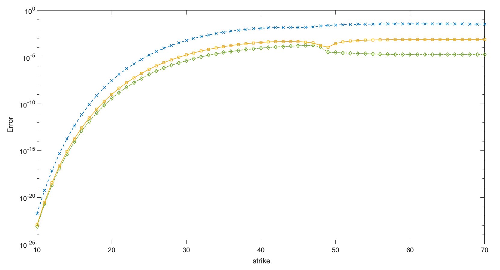
(b) Approximation error of the American put value with respect to different strikes for various orders of approximation

Note: (a) first order represents $m=1$ in the Hermite polynomial approximation of the transition density; second order represents $m=2$; third order represents $m=3$. (b) the blue curve is the relative error in approximating the price with first order accuracy of the approximation of the transition density; yellow curve is that for second order accuracy; green curve is that for third order accuracy

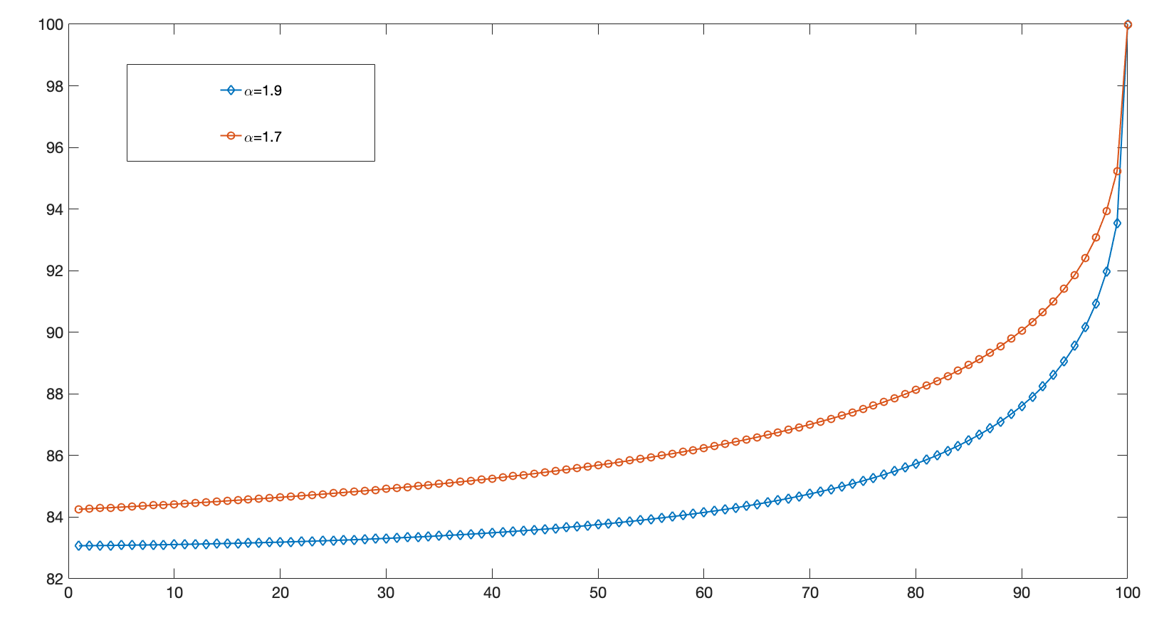
Figure A5: The Exercise Boundary of American Put in the CEV Model

Note: The horizontal axis represents the 100 steps. That is, 100 in the horizontal axis means the time at maturity. The vertical axis represents the price. $K=100$, $r=6/100$, $\delta=r/2$, $\sigma=\sqrt{10}/5$, $S_{0}=40$, and $T=1$.

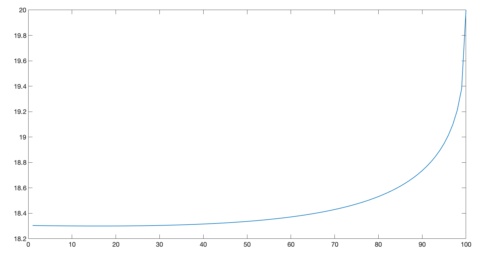
Figure A6: The Exercise Boundary of American Put in the NMR Model

Note: The horizontal axis represents the 100 steps. That is, 100 in the horizontal axis means the time at maturity. The vertical axis represents the price. $a=500$, $b=5$, $c=0.05$, $v=-0.05$, $\sigma=0.2$, $\gamma=3/2$, $K=20$, $r=5/100$, $\delta=0$, $S_{0}=20$, and $T=0.0833$.

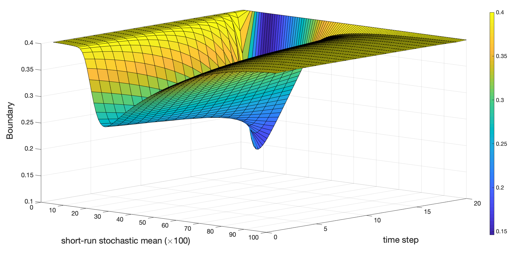
Figure A7: The Exercise Boundary of American Put in the DMR Model

Note: The exercise boundary is approximated with 20 steps on time and 100 steps on $y$ for $y$ in $[0,1]$. $K=40/100$, $r=4.88/100$, $\delta=0$, $\sigma=0.25$, $\kappa=0.2$, $\beta=2.5$, $\xi=4$, $\alpha=0.25$, $T=0.5$

Figure A8: The Exercise Boundary of American Put in Merton’s Jump-Diffusion Model for $\lambda=1/100,10/100,$ and $25/100$

Note: The exercise boundary is approximated with 50 steps. $K=40$, $r=4.88/100$, $\sigma=0.2$, $\mu_{J}=0$, $\sigma_{J}=0.2$, $S_{0}=40$, and $T=0.5$.

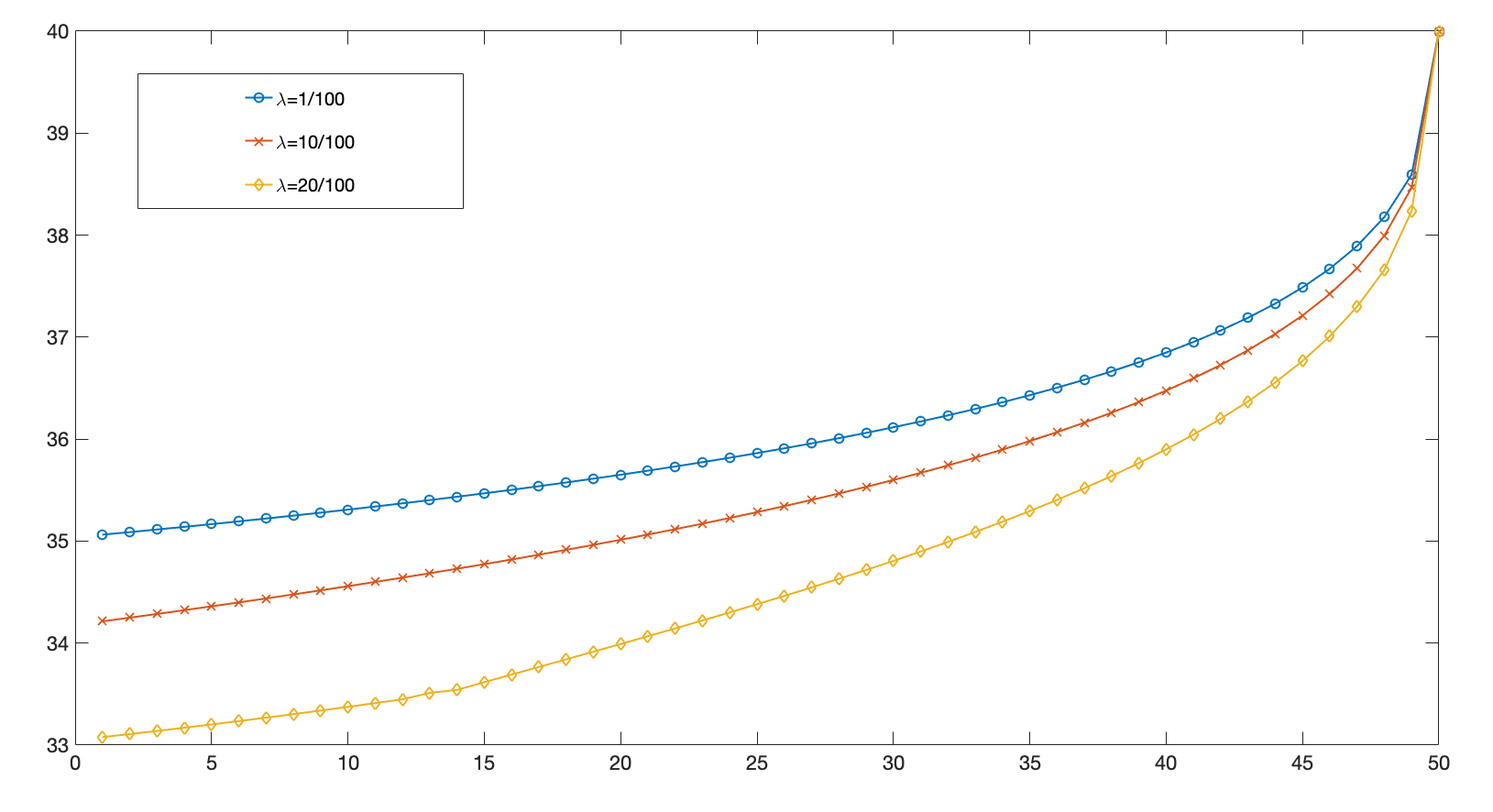
Figure A9: The Exercise Boundary of American Put in Kou’s Jump-Diffusion Model for $\lambda=1/100,10/100,$ and $20/100$

Note: The exercise boundary is approximated with 50 steps. $K=40$, $r=4.88/100$, $\delta=0$, $\sigma=0.2$, $p=0.04$, $q=0.96$, $\eta_{1}=3.7$, $\eta_{2}=1.8$, $S_{0}=40$, and $T=0.5$.

References

- 1 Aït-Sahalia, Y. (1996): Testing continuous-time models of the spot interest rate, Review of Financial Studies 9, 385–426.
- 2 Aït-Sahalia, Y. (1999): Transition densities for interest rate and other nonlinear diffusions, The Journal of Finance 54, 1361–1395.
- 3 Aït-Sahalia, Y. (2002): Maximum-likelihood estimation of discretely-sampled diffusions: a closed-form approximation approach, Econometrica 70, 223–262.
- 4 Aït-Sahalia, Y. (2008): Closed-form likelihood expansions for multivariate diffusions, Annuals of Statistics. 36, 906–937.
- 5 Aït-Sahalia, Y. and R. Kimmel (2007): Maximum likelihood estimation of stochastic volatility models, Journal of Financial Economics. 83, 413–452.
- 6 Aït-Sahalia, Y. and R. Kimmel (2010): Estimating affine multifactor term structure models using closed-form likelihood expansions, Journal of Financial Economics, 98, 113–144.
- 7 Amengual, D. (2008): The Term Structure of Variance Risk Premia, Tech. Rep. Princeton University.
- 8 Breen, R. (1991): The Accelerated Binomial Option Pricing Model, Journal of Financial and Quantitative Analysis, 26, 153–164.
- 9 Broadie, M. and J.B. Detemple (2004): Option Pricing: Valuation Models and Applications, Management Science 50(9):1145-1177
- 10 Carr, P., R. Jarrow, and R. Myneni (1992): Alternative characterizations of American put options, Mathematical Finance 2 87–106.
- 11 Cox, J.C., S.A. Ross and M.Rubinstein (1979): Option Pricing: A Simplified Approach, Journal of Financial Economics, 7, 229–263.
- 12 Detemple, J. (2006): American-style derivatives : valuation and computation, Chapman & Hall/CRC
- 13 Detemple, J., and W. Tian (2002): The valuation of American options for a class of diffusion processes, Management Science. 48 917–937.
- 14 Detemple, J., and Y. Kitapbayev, (2018): On American VIX options under the generalized 3/2 and 1/2 models, Mathematical Finance 28 (2), 550-581
- 15 Egloff, D., M. Leippold, and L. Wu (2010): The term structure of variance swap rates and optimal variance swap investments, Journal of Finance and Quantitative Analysis, 45, 1279–1310.
- 16 Egorov, A.V., H. Li, and Y. Xu (2003): Maximum likelihood estimation of time inhomogeneous diffusions, Journal of Econometrics, 114, 107–139.
- 17 Eraker, B., and J. Wang (2012): A Non-Linear Dynamic Model of the Variance Risk Premium, Tech. Rep.. University of Wisconsin-Madison.
- 18 Gallant, A., and G. Tauchen (1998): Reprojecting partially observed systems with an application to interest rate diffusions, Journal of the American Statistical Association, 93, 10–24.
- 19 Geske, R., and H. Johnson (1984) The American put option valued analytically, The Journal of Finance, 39 1511–1524.
- 20 Gukhal, C.R. (2001): Analytical valuation of American options on jump-diffusion processes, Mathematical Finance 11(1) 97–115.
- 21 Huang, J., M. Subrahmanyam, and G. Yu (1996): Pricing and Hedging American Options: A Recursive Integration Method, Review of Financial Studies, 9, 277–330.
- 22 Jacka, S.D. (1991): Optimal stopping and the American put, Mathematical Finance 1 1–14.
- 23 Jacka, S.D., and J.R. Lynn (1992): Finite-horizon optimal stopping, obstacle problems and the shape of the continuation region, Stochastics and Stochastic Reports 39, 25–42.
- 24 Ju, N. (1998): Pricing an American Option by Approximating Its Early Exercise Boundary as a Multi-Piece Exponential Function, Review of Financial Studies, 11, 627–646.
- 25 Kim, I.J. (1990): The analytic valuation of American options, Review of Financial Studies, 3 547–572.
- 26 Kou, S.G. (2002): A jump-diffusion model for option pricing, Management Science, 48 1086–1101.
- 27 Mencia, J., and E. Sentana (2009): Valuation of VIX Derivatives, Tech. Rep. 0913. CEMFI.
- 28 Merton, R.C. (1976): Option pricing when underlying stock returns are discontinuous, Journal of Financial Economics, 3 125–144.
- 29 Myneni, R. (1992): The Pricing of the American Option, Annals of Applied Probability, 2, 1–23.
- 30 Rutkowski, M. (1994) The early exercise premium representation of foreign market American options, Mathematical Finance 4 313–325.
- 31 Xiu, D. (2014): Hermite polynomial based expansion of European option prices, Journal of Econometrics, 179, 158-177
- 32 Yu, J. (2007): Closed-form likelihood approximation and estimation of jump-diffusions with an application to the realignment risk of the Chinese yuan, Journal of Econometrics, 141, 1245–1280.