High-dimensional near-optimal experiment design for drug discovery via Bayesian sparse sampling

Abstract

We study the problem of performing automated experiment design for drug screening through Bayesian inference and optimisation. In particular, we compare and contrast the behaviour of linear-Gaussian models and Gaussian processes, when used in conjunction with upper confidence bound algorithms, Thompson sampling, or bounded horizon tree search. We show that non-myopic sophisticated exploration techniques using sparse tree search have a distinct advantage over methods such as Thompson sampling or upper confidence bounds in this setting. We demonstrate the significant superiority of the approach over existing and synthetic datasets of drug toxicity.

1 Introduction

We consider the problem of optimal adaptive experiment design in high-dimensional spaces. Informally, this is the problem of designing an adaptive policy for performing a sequence of experiments, so as to validate one or more hypothesis. For example, what sequence of observations should an astronomer take to best detect inhabitable planets? How should experimental treatments be adaptively allocated to patients so as to minimise adverse side effects and maximise the chances of discovering the best one?

In this paper, we are primarily interested in finding one molecule that has optimal characteristics as defined by the read out from experiments conducted with this molecule. The idea is to mimic the drug-discovery process until the point where a candidate drug is selected. A candidate drug is a molecule that meets certain criteria; it needs to be transported to the therapeutic target, it needs to affect the target in a way that is good for patients and it can not cause the patients any other harm.

We adopt the setting of sequential experimentation, whereby we test one or more drugs, observe their effects and update our beliefs, and then perform another test. This can be formalised as a type of bandit problem DeGroot (1970); Chernoff (1966, 1959); Lai and Robbins (1985), where at time $t$ the decision maker takes an action $x_{t}\in X$, which corresponds to performing a specific experiment, observes a result $y\in Y$, which corresponds to obtaining a measurement, and obtains a reward $r_{t}$. The decsion maker is interested in maximising the utility $U=\sum_{t=1}^{T}r_{t}$, defined as the total reward until the end of the game $T$. We adapt the same general framework, but typically the rewards for $t<T$ are small negative values that reflect the cost of experimentation. However, the reward at the last stage, $r_{T}$, is chosen to reflect the usefulness of the information collected so far.We define the reward more precisely in Section 1.1.

1.1 Setting

We adopt the standard Bayesian setting where we have a candidate family of (conditional) densities $\{p_{\theta}\mid\theta\in\Theta\}$, parameterised by $\theta$ . Each $p_{\theta}(y\mid x)$ defines a density over $Y$ for every $x\in X$. If $\theta$ is known, then $p_{\theta}$ describes everything known about the problem. However, since we do not know $\theta$, we first select some distribution $\xi_{0}$ on $\Theta$, representing our prior belief about the unknown parameter. Through Bayesian updating, we condition on the evidence, so that after $t$ experiments and observations we obtain a new belief $\xi_{t}$ on the family indexed by $\Theta$.

In particular, in our setting we take a sequence of actions $x^{t}=x_{1},\ldots,x_{t}$ with $x_{t}\in X$ and obtain a corresponding sequence of outcomes $y^{t}=y_{1},\ldots,y_{t}$ with $y_{t}\in Y$. As is standard, we define the posterior belief at time $t$ to be the probability measure

$$\xi_{t}(B) \triangleq\xi_{0\mid x^{t},y^{t}}(B)\triangleq\xi_{0}(B\mid x^{t},y^{t})$$ (1)

$$=\frac{\int_{B}p_{\theta}(y^{t}\mid x^{t})\,\mathrm{d}\xi_{0}(\theta)}{p_{\xi_{0}}(y^{t}\mid x^{t})}, B\subset\Theta,$$ (2)

where we use $p_{\xi_{0}}(y^{t}\mid x^{t})=\int_{\Theta}p_{\theta}(y^{t}\mid x^{t})\,\mathrm{d}\xi_{0}(\theta)$ to denote the marginal density under $\xi_{0}$ and also introduce the convenient notation $\xi_{0\mid x^{t},y^{t}}$ to denote a particular belief conditioned on specific observations.

In our case in particular, we are performing Gaussian Process (GP) inference. Thus, $\Theta$ indexes a function space $F=\left\{\,f_{\theta}~{}\middle|~{}\theta\in\Theta\,\right\}$ and we assume that our observations follow a Gaussian distribution with variance $\sigma^{2}$ around the mean function $f$, i.e. that

$$y=f_{\theta}(x)+\mathcal{N}(0,\sigma),$$ (3)

with expected value $\mathop{\mbox{$\mathbb{E}$}}\nolimits_{\theta}(y\mid x)=f_{\theta}(x)$. In addition, any belief $\xi$ defines the corresponding expectation $\mathop{\mbox{$\mathbb{E}$}}\nolimits_{\xi}(y\mid x)=\int_{\Theta}f_{\theta}(x)\,\mathrm{d}\xi(\theta)$.

We are interested in maximising the utility in expectation, under our belief at each step. Here, we assume that the utility is an additive function, is defined as

$$U_{t}=\sum_{k=t}^{T}r_{t},$$

with rewards $r_{t}=\rho_{t}(x_{t},y_{t},\xi_{t})$ that can depend on the current time, action, outcome and belief. The choice of reward function is problem-dependent, but in the experiment design setting there are thee standard choices: (a) When there is an inherent reward for each observed outcome $\rho(y_{t})$, in which case we can simply set $\rho_{t}(x_{t},y_{t},\xi_{t})=\rho(y_{t})$. This is the usual bandit setting. (b) When we wish to find the best arm in the set as efficiently as possible. This can be modelled as $r_{t}=-c(x_{t})$, where $c$ describes the cost of taking a particular action. for $t<T$, while the final reward is the expected value of the best arm

$$r_{T}=\max_{x}\mathop{\mbox{$\mathbb{E}$}}\nolimits_{\xi_{t}}(\rho(y_{t})\mid x_{t}=x).$$

(c) The final choice is to try to learn as much as possible about the correct parameter. This can be modelled through maximising the KL divergence between the posterior and prior, so that $r_{t}=-c(x_{t})$ and $r_{T}=D(\xi_{T}\|\xi_{0})$ and in fact maximises the expected information gain, while taking into account the cost of experimentation.

In this paper, an action corresponds to the choice of a specific drug to test, and the outcome is the result of the test. We always use a Gaussian process to model the distribution of outcomes $y_{t}$ given drugs $x_{t}$. At any given time $t$, the process is denoted $\xi_{t}$. However, maximising expected utility is intractable. In this paper, we use a sparse lookahead to approximate the optimal solution, and we show that this significantly outperforms other approximations, such as Thompson sampling and upper confidence bound policies.

2 Related work

Bandit problems are one of the most classical problems in resource allocation. For finite armed problems (Lai and Robbins, 1985) showed that the regret must grow logarithmically in the number of trials. Subsequently, Burnetas and Katehakis (1996) proved the existence of index-based optimal adaptive policies and constructed examples for e.g. distributions with finite support, while Auer et al. (2002) constructed optimal policies for bounded distributions. However, in our case the allocation problem is budgeted (Madani et al., 2004), and so we are not interested in the cumulative regret. Specifically, our horizon is so short compared to the number of arms that many times not all arms are explored.

To handle the budget in our work, we define a fixed cost for each trial. However, one could also use an information-based stopping condition, as explored by Burnetas and Katehakis (2003). In that case the algorithm could decide for itself when a sufficient amount of information has been attained from the trials and could then terminate. While this is the right thing to do if the objective is to find the best arm, our cost constraints do not favour such an approach.

There has also been a lot of work on the connection between GPs and bandits. Srinivas et al. (2010) combined the Upper Confidence Bound policy with Gaussian processes to obtain the GP-UCB policy. This policy uses the mean $\mu_{x}$ and variance $\sigma_{x}$ for each bandit context $x$ in the GP $\xi_{t}$ and sum them together. It then selects and plays the bandit that maximizes this sum as per $x\in\mathop{\rm arg\,max}\limits_{x\in X}\mu_{x}+\sqrt{\beta_{t}}\sigma_{x}$. The variance is scaled by a factor $\sqrt{\beta_{t}}$ that varies with time and is used to handle the exploitation-exploration trade-off. This factor is set to be $\beta_{t}=2\log(|D|t^{2}\pi^{2}/6\delta)$ in this work since this works well if $D$ is finite, which it is for the data sets used in this work. After observing the result of playing the selected bandit the current belief is updated by letting the GP learn the new point as $\xi_{t+1}=\xi_{t\mid x_{t},y_{t}}$.  Srinivas et al. (2010) use this policy to try to find the most congested part of a highway.

In some cases, a linear model might be sufficient to represent the reward of different arms. Recently, linear bandits with Thompson sampling (LB-TS) were used by  Agrawal and Goyal (2012) for the contextual bandit problem. Their policy keeps track of the mean $\hat{\mu}$ of the observed contexts and samples another mean $\tilde{\mu}\sim\mathcal{N}(\hat{\mu},v^{2}B^{-1})$. $v$ is a scaling factor used to make certain that the exploitation-exploration trade-off is handled well and is set to $v=R\sqrt{\frac{24}{\epsilon}d\ln\frac{1}{\delta}}$. The $R$ is data dependent and $\delta$ is an algorithm parameter. $B$ is simply a matrix of the contexts, $B=x_{t,i}x_{t,i}^{T}$. The bandit that is selected is $i\in\mathop{\rm arg\,max}_{i}x_{t,i}^{T}\tilde{\mu}$. We can apply their algorithm in our problem; and since the horizon $T$ is known beforehand we can set $\epsilon=\frac{1}{\ln T}$ as in Agrawal and Goyal (2012).

The setting we consider, is similar to that of King et al. (2004). However it also has a number of other challenges, mainly to do with the large dimensionality of $X$, which is a finite subset of a high dimensional Euclidean space.

To combat the curse of dimensionality, we use compressed sensing (Carpentier and Munos, 2012) to make high-dimensional feature space smaller. This effectively means way multiplying the input matrix data with a lower dimensional Gaussian matrix. This maintains the distances between the points with high probability and does not have a bad effect on performance.

Tree search methods for bandit problems has previously been explored by Wang et al. (2005), who proposed Bayesian sparse sampling (BSS) as an action selection method. In their paper, they compare BSS to more traditional methods such as $\epsilon$-greedy, Boltzmann exploration and Thompson sampling. Their results show that BSS outperforms all other methods by a significant margin using a GP model, at least for low-dimensional problems.

Our contribution.

In this work, we explore two different tree search methods for the case of when there are numerous actions embedded in a high-dimensional space. We are particularly interested in the drug development application, wherein action selection is batch, because it is significantly cheaper and faster to test many drug compounds at the same time. For this reason, we develop a Thompson ranking algorithm and integrate it within tree search. We also show that batch actions have a significant side benefit. They very effectively deepen the search horizon while reducing the branching factor of the search tree, and consequently have a better performance than purely sequential methods.

3 Sparse GP-tree lookahead policy

In this paper, we approximate the optimal adaptive experiment design through sparse lookahead tree search. The tree is constructed in the space of possible future beliefs, with the root node being the current belief. All the beliefs are expressed as Gaussian process. At each stage of the tree, we define the reward in a way that corresponds to the problem definition, as specified in Section 1.1. This then a Markov decision process (MDP), with a state space corresponding to the set of possible information states (i.e. beliefs). Since there set of such states is unbounded, we employ sampling-based approximations to make planning tractable.

Let us start by defining the value function of the exact MDP. If $\xi_{t}$ is our belief at some node at depth $t$ of the tree, the value function (i.e. the utility of the optimal policy) is:

$$V_{t}(\xi_{t})=\max_{\pi}\mathop{\mbox{$\mathbb{E}$}}\nolimits_{\xi_{t}}(U_{t}\mid\pi).$$ (4)

Via backwards induction, we can define the following recursion for calculating the value function

$$V_{t}(\xi_{t}) =\max_{x\in X}Q_{t}(\xi_{t},x)$$ (5)

$$Q_{t}(\xi_{t},x) =\int_{Y}\left\{r_{t}(\xi_{t},x,y)+V_{t+1}(\xi_{t\mid x,y})\right\}p_{\xi_{t}}(y\mid x)\,\mathrm{d}y$$ (6)

$$V_{T}(\xi_{t}) =r_{t}(\xi_{t})$$ (7)

where $x\in X$ is the experiment we wish to perform and $\xi_{t\mid x,y}$ is the belief $\xi_{t}$ conditioned on $x,y$, i.e.

$$\xi_{t\mid x,y}(\cdot)=\xi_{t}(\cdot\mid x,y)$$ (8)

The problem in the GP setting is that $X$ is very large and that $Y$ is infinite in size. For that reason, we shall replace the first step of the recursion with

$$\hat{V}_{t}(\xi_{t}) =\max_{x\in X(\xi_{t})}\hat{Q}_{t}(\xi_{t},x)$$ (9)

$$X(\xi_{t}) \sim\textrm{Thompson}^{N}(\xi_{t})$$ (10)

where $X(\xi_{t})$ is a set of $N$ Thompson samples from the process $\xi_{t}$. This lets us focus on a few promising actions; the same idea was used by Wang et al. (2005) to perform Bayesian sparse sampling.

We use Thompson sampling in two ways in this work. Thompson sample rank is used in the batch version of the policy to quickly find a set of candidates for a single function. Independent Thompson sampling without replacement is used in all cases where testing is done sequentially.

Thompson sample rank.

By $X(\xi_{t})\sim\textrm{Thompson}^{N}(\xi_{t})$, and we mean the following process. We sample $\theta\sim\xi_{t}$ to obtain the function $f_{\theta}$. We create a permutation $X^{\theta}$ of candidate drugs $X$ and rank them so that $f_{\theta}(x^{\theta}_{i})\geq f_{\theta}(x^{\theta}_{j})$ for any $x_{i}^{\theta},x^{\theta}_{j}\in X$ such that $i<j$. Then we select the top $N$ drugs according to the sampled $\theta$, $X(\xi_{t})=\{x_{1},\ldots,x_{N}\}$.

Independent Thompson sampling without replacement.

If we perform independent Thompson sampling, we write $X(\xi_{t})\sim\textrm{Thompson}^{N}(\xi_{t})$, and we mean the process whereby: For each $x_{k}(\xi_{t})\in X(\xi_{t})$, with $k=1,\ldots,N$, we draw an independent sample $\theta_{k}\sim\xi_{t}$ and set $x_{k}(\xi_{t})=\mathop{\rm arg\,max}_{x}\mathop{\mbox{$\mathbb{E}$}}\nolimits_{\theta_{k}}[f\mid x]$.

The second step of the process involves the integration, but this is much simpler. We can simply approximate the integral by Monte Carlo sampling:

$$\hat{Q}_{t}(\xi_{t},x) =\sum_{y\in Y(\xi_{t})}r_{t}(\xi_{t},x,y)+\hat{V}_{t+1}(\xi_{t\mid x,y}),$$ (11)

$$Y(\xi_{t}) \sim P^{M}(y\mid x,\xi_{t}).$$ (12)

4 Data

The data used to test the performance of the algorithms developed in this work consists of molecules in their graphical structure, identified by their signature descriptors as described in Jean-Loup Faulon* and Donald P. Visco, Jr. and and Ramdas S. Pophale (2003). An example of a molecule and corresponding signature descriptors are illustrated in Figure 1 and Table 1. These signature descriptors are then mapped into high-dimensional space.

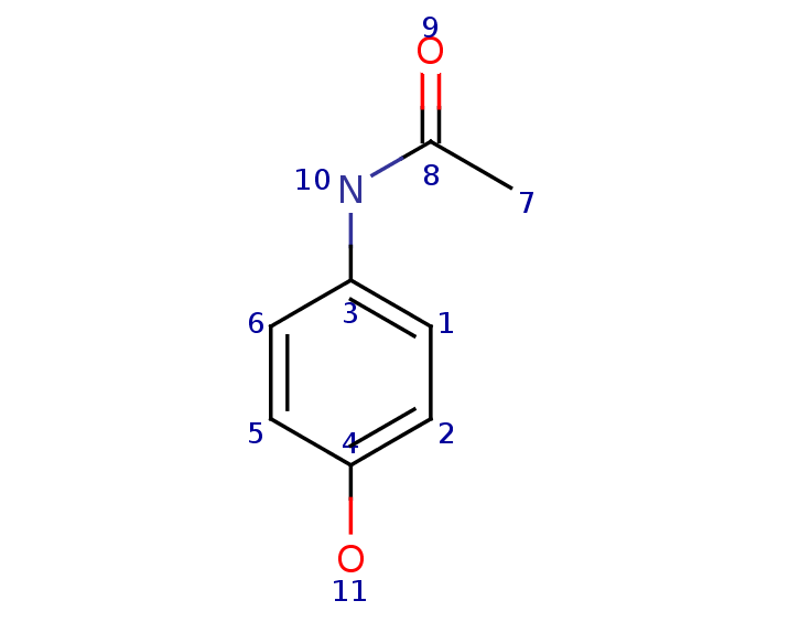
Figure 1: Paracetamol is a drug molecule for treatment of pain and fever. The atom numbers are displayed in this figure.

Atom number	Height $0$	Height $1$
1	[C]	[C]([C]=[C])
2	[C]	[C]([C]=[C])
3	[C]	[C]([C]=[C][N])
4	[C]	[C]([C]=[C][O])
5	[C]	[C]([C]=[C])
6	[C]	[C]([C]=[C])
7	[C]	[C]([C])
8	[C]	[C]([C][N]=[O])
9	[O]	[O](=[C])
10	[N]	[N]([C][C])
11	[O]	[O]([C])

Table 1: The signature descriptors of two different heights for paracetamol.

Each molecule also has its corresponding -log IC₅₀ value. IC₅₀ denotes how much concentration is required to inhibit a process by half. The datasets are patented molecules retrieved from GOSTAR databases Ltd (2012). We have used two different datasets; CDK5, which describes different molecules’ inhibition of the cyklin-dependent kinase 5 (CDK5), and MGLL, which is other molecules’ inhibition of the monoacylglycerol lipase (MGLL). The CDK5 data set comes with IC₅₀ values in the range $[4.6,8.0]$. The MGLL data set comes with IC₅₀ values in the range $[4.8,8.4]$. So each of the drugs in the data sets come in the form of a $(x_{n},y_{n}^{*})$ pair where $x_{n}$ is the nth bandit’s context and $y_{n}^{*}$ is its corresponding actual reward.

In addition to this, we generate a synthetic data set using the other two data sets by letting a GP learn the points in those data sets and then predict values for new, unknown points.

The data is compressed using Compressed sensing as mentioned in Section 2, the results in Figure 2 show that any accuracy loss compared to not using Compressed sensing is minor.

Figure 2: A comparison of the main algorithm ran on data pre-processed with Compressed sensing and without

The metrics used to compare the performance of the algorithms are the average regret (14) and the simple regret (15). For these data sets we use definition (a) definition for the utility function and let the actual reward be $r_{i,t}=y_{i}^{*}$. Let $r^{*}_{t}=\max_{i}y_{i}^{*}$. We then define the (instantaneous) regret to be the difference from the reward $r_{i,t}$ and the optimal reward $r^{*}_{t}$. Since the rewards are fixed for each drug this can be simplified to

$$R_{T}=r^{*}_{t}-r_{i,t}.$$ (13)

The average regret is used to compare how well the algorithms manage to identify and select the best drugs in the data set.

$$\bar{R}_{T}=\sum_{t=1}^{T}\frac{r^{*}-r_{i,t}}{T}.$$ (14)

The simple regret is used to compare how well the algorithms manage to identify and select the best drug in the data set.

$$R^{*}_{T}=r^{*}-r_{i,t}.$$ (15)

Internally, the reward measures when optimizing for $\mathbb{E}R^{*}_{T}$ are slighty different than from when we optimize for $\mathbb{E}\bar{R}_{T}$. All intermediary nodes have their reward set to zero as we only care about the reward at the end. So Equation 11 becomes the following instead,

$$\hat{Q}_{t}(\xi_{t},x) =\sum_{y\in Y(\xi_{t})}\hat{V}_{t+1}(\xi_{t\mid x,y}).$$ (16)

The two regret measures describe two significantly different optimization strategies of the problem. What is most desired depends on the context but generally it is desired to minimize $\mathbb{E}R^{*}_{T}$ in the case where the single most promising drug is to be discovered and $\mathbb{E}\bar{R}_{T}$ where the goal is to identify multiple promising drugs. The work by Bubeck et al. (2011) show that a single policy can not guarantee optimal $\mathbb{E}R^{*}_{T}$ and $\mathbb{E}\bar{R}_{T}$ bounds at the same time so each policy is run twice, each with one of the optimization goals in mind.

5 Algorithms

The GP-Thompson Policy, as shown in Algorithm (1) is used to test whether there is a increase in performance or not by using the lookahead.

Algorithm 1 GP-Thompson Policy

  input prior $\xi_{0}$, actions $X$

  for all $t=1,2,...,T$ do

     Play arm $x_{t}\in\mathop{\rm arg\,max}\limits_{x\in X(\xi_{t})}f(x)\sim\xi_{t}$

     Observe outcome $y_{t}$ and reward $r_{t}$

     Update belief $\xi_{t+1}=\xi_{t\mid x_{t},y_{t}}$.

  end for

The algorithm approximates the rewards that would be acquired by taking each of the actions in turn by using Thompson sampling. It then selects and carries out the action that is deemed the best from the sampling. The actual reward is then observed and learned by the GP. The $\xi_{0}$ parameter is the prior belief before any actions have been taken and rewards observed. $\xi_{t}$ reflects policy’s state of belief at time $t$ and $X$ the set of possible actions to carry out.

Algorithm (2) describes the main policy used in this work. The policy is further expanded in Algorithm (5) to handle batch testing. However, initially we just consider sequential testing with one action being taken at each time step.

Algorithm 2 GP-Tree Policy

  input horizon $h$, branches $K$, samples $n$, prior $\xi_{0}$, actions $X$, depth $0pt$

  for all $t=1,2,...,T$ do

     Play arm $x\in\mathop{\rm arg\,max}\limits_{x\in X(\xi_{t})}$ descendQ($\xi_{t}$,$x$,$0pt=0$,$h$,$K$)

     Observe outcome $y_{t}$ and reward $r_{t}$

     Update belief $\xi_{t+1}=\xi_{t\mid x_{t},y_{t}}$.

  end for

Algorithm 3 descendQ

  input horizon $h$, branches $K$, samples $n$, GP $\xi_{t}$, actions $X$, action $x$, depth $0pt$

  for all $k=1,2,...,K$ do

     $y_{t,k}\leftarrow f(x)\sim\xi_{t}$

     Update belief $\xi_{t+1,k}=\xi_{t\mid x_{t},y_{t,k}}$.

     $\hat{Q}_{t,k}(\xi_{t+1,k},x)=$ descendV$(\xi_{t+1,k},x,0pt+1,h,K)$

  end for

  return $\sum_{k=1}^{K}\frac{\hat{Q}_{t,k}(\xi_{t+1,k},x)}{k}$

Algorithm 4 descendV

  input horizon $h$, branches $K$, samples $n$, GP $\xi_{t}$, actions $X$, action $x$, depth $0pt$

  if $0pt=h$ then

     return $\max\limits_{x\in X}f(x)\sim\xi_{t}$

  else

     return $\max\limits_{x\in X}$ descendQ($\xi_{t}$,$x$,$0pt$,$h$,$K$)

  end if

The GP-Tree Policy is built on the same idea as the GP-Thompson policy, however, we now also consider the non-myopic effects of taking the actions. We select and carry out an action and then we let our current belief state $\xi_{t}$ learn the predicted reward of taking that action. We can then move to a new belief state $\xi_{t+1}$ and from there on select and take the actions using $\xi_{t+1}$ instead of $\xi_{t}$. This process is then continued, sampling and carrying out $n$ actions at each time step as well as branching our belief state into $K$ several belief states $\xi_{t,1},\xi_{t,2},...,\xi_{t,K}$ each with their predicted reward $y_{t,1},y_{t,2},...,y_{t,K}$, until the horizon $h$ is reached which is when the predicted accumulated rewards in the tree will propagate back to our actual time step. The policy is then able to take the action that is not only the most promising at this moment but also the one that will give the best results in the future, as predicted by $\xi_{t}$. So in fact we build a balanced search tree of width $nK$ and height $h$.

Algorithm 5 Batch GP-Tree Policy

  input horizon $h$, branches $K$, samples $n$, prior $\xi_{0}$, actions $X$, depth $0pt$, batch size $b$

  for all $t=1,2,...,\frac{T}{b}$ do

     Play arms $\boldsymbol{x}\in\mathop{\rm arg\,max}\limits_{\boldsymbol{x}\in X(\xi_{t})}$ descendQ($\xi_{t}$,$\boldsymbol{x}$,$0pt=0$,$h$,$K$)

     Observe outcomes $\boldsymbol{y}_{t}=y_{t},y_{t+1},...y_{t+b}$ and rewards $\boldsymbol{r}_{t}=r_{t},r_{t+1},...r_{t+b}$

     Update belief $\xi_{t+b}=\xi_{t\mid\boldsymbol{r}_{t},\boldsymbol{y}_{t}}$.

  end for

One of the main drawbacks with this policy is that it is fairly computationally expensive since the number of nodes to explore grows rapidly with further horizons. To combat this we extend the GP-Tree Policy to Batch GP-Tree Policy as can be seen in Algorithm (5). The idea is the same however instead of taking a single action $x$ at time step $t$ we take $b$ actions at the same time. This means that we expand the action space from $x\in X$ to $\boldsymbol{x}\in X^{b}$. The reasoning for this is that we do not have to consider the effect on the belief of taking every action sequentially and instead how a series of actions affect the belief state. This is also how drug testing in experiment design is done in reality. By doing this change we can have higher values on our $h$, $K$, $n$ parameters compared to the GP-Tree Policy and still have the policy finish in reasonable time.

6 Results

The methods are run on three different data sets, one small (CDK5, see Figure 3), one large (MGLL, see Figure 4) and one huge (synthetic, see Figure 5). In all the runs on the three data sets, information about one drug is initially shown and then for the remaining $T-1$ iterations the policies have to decide for themselves which drugs should be tested. Results given by the main policies studied in this work have dashed lines and those that they are compared to are in solid lines.

The algorithm parameters were obtained through empirical testing on firstly, a small function optimization problem and later on a small drug data set. For policies that are time expensive, most notably all tree search policies, had their parameters tuned in such a way so the evaluation of all of them takes about the same amount of time. The methods may have one set of parameters for each optimization goal.

Some settings are consistent throughout all the runs and they will be gone over here. The problem horizon $T$ is the limit of the number of molecules that can be tested in a single experiment and is set as $T=100$ for all runs. The Gaussian processes $\xi$ that are used are using a RBF kernel to measure similarity between contexts and $\xi$ has internal signal noise and noise variance of $0.1$. GP-UCB uses $\beta_{t}=2\log(|D|t^{2}\pi^{2}/6\delta)$, as in  Srinivas et al. (2010).

(a) Average cumulative regret

(b) Simple regret

Figure 3: Results on the CDK5 data set)

Next are the data specific settings. As a result of the sheer size of the two larger data sets, these parameters have to be tuned carefully in order for the methods to evaluate in reasonable time and also to give the methods a chance to learn the data. Batch GP-Tree Policy is run with the following configuration on the CDK5 data set, $b=5$, $n=100$, $K=4$, $h=1$. GP-Tree Policy is run with the same settings as in the batch case apart from the number of Thompson samples, which is $n=20$ in this case. The GP-BSS Policy is run with the parameters $\textsf{budget}=800$, $\rho=0.5$. The GP-UCB Policy and LB-TS Policy both have a separate $\delta$ depending on the optimization goal, here $\delta_{R^{*}_{T}}=0.99$, $\delta_{\bar{R}_{T}}=0.01$ when optimizing for $\mathbb{E}R^{*}_{T}$ and $\mathbb{E}\bar{R}_{T}$, respectively. The results when optimizing for $\mathbb{E}\bar{R}_{T}$ are presented in Figure 3(a).

As the MGLL data set is much larger than the CDK5 data set, some parameters are now changed to speed up the evaluation. These are $b=10$ for Batch GP-Tree Policy, $n=10$ for GP-Tree Policy and $\textsf{budget}=400$ for GP-BSS Policy. The results when optimizing for $\mathbb{E}\bar{R}_{T}$ are presented in Figure 4(a).

(a) Average cumulative regret

(b) Simple regret

Figure 4: Results on the MGLL data set

Finally, since the amount of data available in the data sets is relatively small, we also worked with a larger, synthetic data set. This was created by training a GP model on the complete data, and then generating samples from the GP for 3000 points. All the GP based policies are too slow evaluate on this data set apart from the Batch GP-Tree Policy with sufficient batch size. The settings on the synthetic data set have the following changes, $b=200$, $n=40$ and $K=2$. Results are shown in Figure 5(a) when optimizing for $\mathbb{E}\bar{R}_{T}$.

(a) Average cumulative regret

Figure 5: Results on the synthetic data set

7 Conclusions

We have shown that the two tree search methods work well in a setting with a large amount of actions in high-dimensional space. In particular, we have shown that the policies are competitive or work better than similar action selection policies, at least in the case of high-dimensional experiment design. We demonstrated the need and effectiveness of batch action selection in this setting when the number of actions is scaled up immensely. With the Batch GP-Tree Policy we can take advantage of the prediction accuracy of the tree search at the same time as we can keep the computational complexity low enough for the problem to be solved in reasonable time.

Future work and further improvements of the two tree search policies will be discussed hereafter.

Empirically proving tight $\mathbb{E}R^{*}_{T}$ bounds. This would require extensive testing since the simple regret of these policies inherently have high variance. Through further testing it would be possible to construct confidence bounds on the simple regret.

Extending the support for batch testing by adaptively changing the batch size depending in some way on how confident the policy is in its predictions. That way it would be possible for the policy a situation when it inevitably has to take some bad actions just to fill out the rest of the batch.

Adding support for multi-objective optimization by finding the Pareto optimal arms. Similar work has been done in Durand et al. for UCB1 and in Yahyaa and Manderick (2015) for Bernoulli bandits.

Adding support for selection over multiple experiments. This could be interesting when there are multiple different labs available to test the drugs. Perhaps some of them are more accurate than others and also have varying costs and durations. The policy should also preferably learn from all the experiments and tests which may lead to a complex situation with many GPs depending on each other. Perhaps the results in Boyle and Frean (2004) could be used for this.

An interesting idea would be to have an adaptive bandit that could change the branching factor and the horizon depending on the number of trials that has been carried out so far. Perhaps having a deeper search tree in the beginning and a wider search tree in the end could lead to greater results.

Another idea is to replace the current Compressed sensing algorithm with a differentially private one as in Li et al. (2011).

Acknowledgments

This work is supported by a Chalmers Information and Communication Technology (ICT) Area of Advance (AoA) SEED (2015–2016) grant.

References

- Agrawal and Goyal (2012) Shipra Agrawal and Navin Goyal. Thompson Sampling for Contextual Bandits with Linear Payoffs. CoRR, abs/1209.3352, 2012. URL http://arxiv.org/abs/1209.3352.
- Auer et al. (2002) Peter Auer, Nicolò Cesa-Bianchi, and Paul Fischer. Finite time analysis of the multiarmed bandit problem. Machine Learning, 47(2/3):235–256, 2002.
- Boyle and Frean (2004) Phillip Boyle and Marcus Frean. Dependent gaussian processes. In Advances in neural information processing systems, pages 217–224, 2004.
- Bubeck et al. (2011) Sébastien Bubeck, Rémi Munos, and Gilles Stoltz. Pure exploration in finitely-armed and continuous-armed bandits. Theoretical Computer Science, 412(19):1832–1852, 2011.
- Burnetas and Katehakis (1996) Apostolos N Burnetas and Michaël N Katehakis. Optimal adaptive policies for sequential allocation problems. Advances in Applied Mathematics, 17(2):122–142, 1996.
- Burnetas and Katehakis (2003) Apostolos N. Burnetas and Michael N. Katehakis. Asymptotic bayes analysis for the finite horizon one armed bandit problem. Probability in the Engineering and Informational Sciences, 17(1):53–82, 2003.
- Carpentier and Munos (2012) Alexandra Carpentier and Rémi Munos. Bandit theory meets compressed sensing for high dimensional stochastic linear bandit. arXiv preprint arXiv:1205.4094, 2012.
- Chernoff (1959) Herman Chernoff. Sequential design of experiments. Annals of Mathematical Statistics, 30(3):755–770, 1959.
- Chernoff (1966) Herman Chernoff. Sequential Models for Clinical Trials. In Proceedings of the Fifth Berkeley Symposium on Mathematical Statistics and Probability, Vol.4, pages 805–812. Univ. of Calif Press, 1966.
- DeGroot (1970) Morris H. DeGroot. Optimal Statistical Decisions. John Wiley & Sons, 1970.
- (11) Audrey Durand, Charles Bordet, and Christian Gagné. Improving the pareto ucb1 algorithm on the multi-objective multi-armed bandit. In NIPS Workshop on Bayesian Optimization.
- Jean-Loup Faulon* and Donald P. Visco, Jr. and and Ramdas S. Pophale (2003) Jean-Loup Faulon* and Donald P. Visco, Jr. and and Ramdas S. Pophale. The Signature Molecular Descriptor. 1. Using Extended Valence Sequences in QSAR and QSPR Studies. Journal of Chemical Information and Computer Sciences, 43(3):707–720, 2003.
- King et al. (2004) Ross D King, Kenneth E Whelan, Ffion M Jones, Philip GK Reiser, Christopher H Bryant, Stephen H Muggleton, Douglas B Kell, and Stephen G Oliver. Functional genomic hypothesis generation and experimentation by a robot scientist. Nature, 427(6971):247–252, 2004.
- Lai and Robbins (1985) Tze Leung Lai and Herbert Robbins. Asymptotically efficient adaptive allocation rules. Advances in applied mathematics, 6(1):4–22, 1985.
- Li et al. (2011) Yang D. Li, Zhenjie Zhang, Marianne Winslett, and Yin Yang. Compressive mechanism: Utilizing sparse representation in differential privacy. In Proceedings of the 10th Annual ACM Workshop on Privacy in the Electronic Society, WPES ’11, pages 177–182, New York, NY, USA, 2011. ACM. ISBN 978-1-4503-1002-4. doi: 10.1145/2046556.2046581. URL http://doi.acm.org/10.1145/2046556.2046581.
- Ltd (2012) GVK Biosciences Private Ltd. Gostar databases 2012. Technical report, Hyderabad, India, 2012.
- Madani et al. (2004) Omid Madani, Danie J. Lizotte, and Russel Greiner. The budgeted multi-armed bandit problem. In Learning Theory: 17th Annual Conference on earning Theory, COLT 2004, volume 3120 of Lecture Notes in Computer Science, pages 643–645. Springer, 2004.
- Srinivas et al. (2010) Niranjan Srinivas, Andreas Krause, Sham Kakade, and Matthias Seeger. Gaussian process optimization in the bandit setting: No regret and experimental design. In ICML 2010, 2010.
- Wang et al. (2005) Tao Wang, Daniel Lizotte, Michael Bowling, and Dale Schuurmans. Bayesian sparse sampling for on-line reward optimization. In ICML ’05, pages 956–963, New York, NY, USA, 2005. ACM. ISBN 1-59593-180-5. doi: http://doi.acm.org/10.1145/1102351.1102472.
- Yahyaa and Manderick (2015) Saba Yahyaa and Bernard Manderick. Thompson Sampling for Multi-Objective Multi-Armed Bandits Problem. In 23th European Symposium on Artificial Neural Networks, ESANN 2015, Bruges, Belgium, April 22-24, 2015, Emerging techniques and applications in multi-objective reinforcement learning, 2015.