Selecting a number of voters for a voting ensemble

Abstract

For a voting ensemble that selects an odd-sized subset of the ensemble classifiers at random for each example, applies them to the example, and returns the majority vote, we show that any number of voters may minimize the error rate over an out-of-sample distribution. The optimal number of voters depends on the out-of-sample distribution of the number of classifiers in error. To select a number of voters to use, estimating that distribution then inferring error rates for numbers of voters gives lower-variance estimates than directly estimating those error rates.

1 Introduction

Voting ensembles of classifiers are a staple of machine learning, including bagging (Breiman, 1996), boosting (Schapire, 1990; Freund and Schapire, 1997), forests of decision trees (Ho, 1995, 1998; Breiman, 2001), and stacking (Wolpert, 1992). Comparative studies show that ensemble classifiers are often the best types of out-of-the-box classifiers (Li, 2010), they win many machine learning competitions (Bennett and Lanning, 2007; Chen and Guestrin, 2016), and they continue to solve practical problems (Zheng et al., 2019; Shahzad and Lavesson, 2013). For a compelling explanation why ensemble classifiers produce good performance, refer to (Dietterich, 2000). For more on selecting ensemble classifiers and ensemble size, refer to (Bonab and Can, 2019; Jackowski, 2018; Gomes et al., 2017; Hernández-Lobato et al., 2013; Oshiro et al., 2012; Yang, 2011; Rokach, 2010, 2009; Tsoumakas et al., 2008; Kuncheva, 2004; Kuncheva et al., 2003; Liu et al., 2004; Hu, 2001; Bax, 1998; Lam and Suen, 1997).

This paper focuses on equally-weighted voting. One extreme is to use all classifiers as voters for every classification. The other is to select a single classifier at random for each classifier. This is sometimes called Gibbs classification. PAC-Bayes error bounds (McAllester, 1999; Langford et al., 2001; Begin et al., 2016) indicate why Gibbs classification can be effective – selecting a Gibbs ensemble that includes 1% of the hypothesis classifiers produces error bounds that are similar to selecting a classifier from a hypothesis set with only 100 classifiers, even if the actual hypothesis set has an arbitrarily large number of classifiers.

Similar to Esposito and Saitta (2004), this paper explores how to select a number of voters for a majority-vote ensemble classifier. That paper shows that the distribution of the number of classifier errors can vary widely over examples in empirical datasets, motivating our analysis of the influence of ensemble size on error rates in such situations. That paper focuses on ensembles of classifiers selected with replacement, allowing a potentially unlimited number of voters. In contrast, this paper focuses on ensembles of classifiers selected without replacement, leading to a different conclusion about the optimal ensemble size, and a statistical method to select the ensemble size based on simultaneous bounds on frequencies of the numbers of classifiers in error.

The next section shows that selecting a single classifier at random for each example can outperform voting over all ensemble classifiers. In Section 3, we show how the distribution of number of ensemble classifiers in error impacts the optimal number of voters, by considering the error curves over numbers of voters for each number of classifier errors as a basis for all possible distribution error curves over numbers of voters. In Section 4, we prove that any number of voters may be optimal. Section 5 discusses methods to select the number of voters, showing that an out-of-sample error estimate based on inference has less variance than direct estimates. Then Section 6 outlines methods to compute out-of-sample error bounds based on inference estimates, including a discussion of challenges for the future.

2 Does voting always help?

To begin, compare worst-case error rate for majority voting over all classifiers to selecting a single classifier at random for each example. Let $m$ be the number of classifiers in the ensemble, and let $p$ be their average error rate. Then the single-classifier strategy has error rate $p$, by linearity of expectations. For the all-voting strategy, the out-of-sample error rate depends on patterns of agreement among the classifiers as well as their out-of-sample error rates. For example, suppose three classifiers each have a 10% error rate. Then, for each pair of classifiers, it is possible that they err together (and the classifier outside the pair is correct) with probability 5%, producing a 15% voting error rate. In general,

Theorem 1.

For $m$ classifiers in an ensemble, with $m$ odd, if the average out-of-sample classifier error rate is $p$, with $p<\frac{1}{2}$, then the maximum possible all-voting error rate is

$$2p\left(1-\frac{1}{m+1}\right).$$ (1)

Proof.

All-voting error is maximized by having the smallest possible majority of voters in error be as probable as the average error bound allows, and otherwise having zero errors. Maximize the probability (call it $\hat{p}$) of the slimmest majority, $\frac{m+1}{2}$, being incorrect, given the constraint that the sum of error rates over classifiers is $mp$:

$$\hat{p}\left(\frac{m+1}{2}\right)=mp,$$ (2)

and solve for $\hat{p}$:

$$\hat{p}=2p\left(1-\frac{1}{m+1}\right).$$ (3)

If $\frac{m+1}{2}$ are incorrect with probability $\hat{p}$ and zero are incorrect with probability $1-\hat{p}$, then $\hat{p}$ is the all-voting error rate. ∎

As $m$ increases, all-voting error rate can approach twice the error rate of selecting a classifier at random, because a voting classifier can have nearly half its classifiers correct and still be incorrect. Discretization can favor the individual.

3 A basis to analyze voting

Now consider ensemble classifiers with (odd) $m$ classifiers, average classifier error rate $p$, and an (odd) number of voters $v$ from one to $m$. Setting $v=1$ gives the single-voter strategy, and $v=m$ gives the all-voting strategy. In this section, we analyze error rate curves over numbers of voters, given numbers of ensemble classifiers incorrect. Those curves form a basis for error rate curves over numbers of voters, in the sense that the weighted sums of those basis curves (with nonnegative weights that sum to one) are all the possible error rate curves over numbers of voters:

Theorem 2.

For an ensemble with $m$ classifiers, for each $i\in\left\{{0,\ldots,m}\right\}$, let $w_{i}$ be the probability that exactly $i$ of the $m$ classifiers are in error for an example drawn at random from an out-of-sample distribution. Then, for subset voting with $v$ classifiers, the average error rate over the out-of-sample distribution is

$$\sum_{i=0}^{m}w_{i}r(m,i,v),$$ (4)

where

$$r(m,i,v)=\sum_{j=\frac{v+1}{2}}^{v}\frac{{{i}\choose{j}}{{m-i}\choose{v-j}}}{{{m}\choose{v}}}$$ (5)

is the expected voting error rate given that $i$ of $m$ classifiers are in error.

Proof.

Voting has average error rate

$$\sum_{i=0}^{m}w_{i}\hbox{Pr}\left\{{\hbox{voting error}|i}\right\},$$ (6)

where $i$ is the number of the $m$ classifiers that are in error. Voting error requires a majority of voters to be in error, so

$$\hbox{Pr}\left\{{\hbox{voting error}|i}\right\}=\sum_{j=\frac{v+1}{2}}^{v}\hbox{Pr}\left\{{\hbox{$j$ voters are in error}|i}\right\},$$ (7)

and

$$\hbox{Pr}\left\{{\hbox{$j$ voters are in error}|i}\right\}=\frac{{{i}\choose{j}}{{m-i}\choose{v-j}}}{{{m}\choose{v}}},$$ (8)

since this is the number of ways to select $j$ voters from the $i$ incorrect ones and $v-j$ voters from the $m-i$ correct ones, divided by the number of ways to select $v$ voters from the $m$ classifiers. ∎

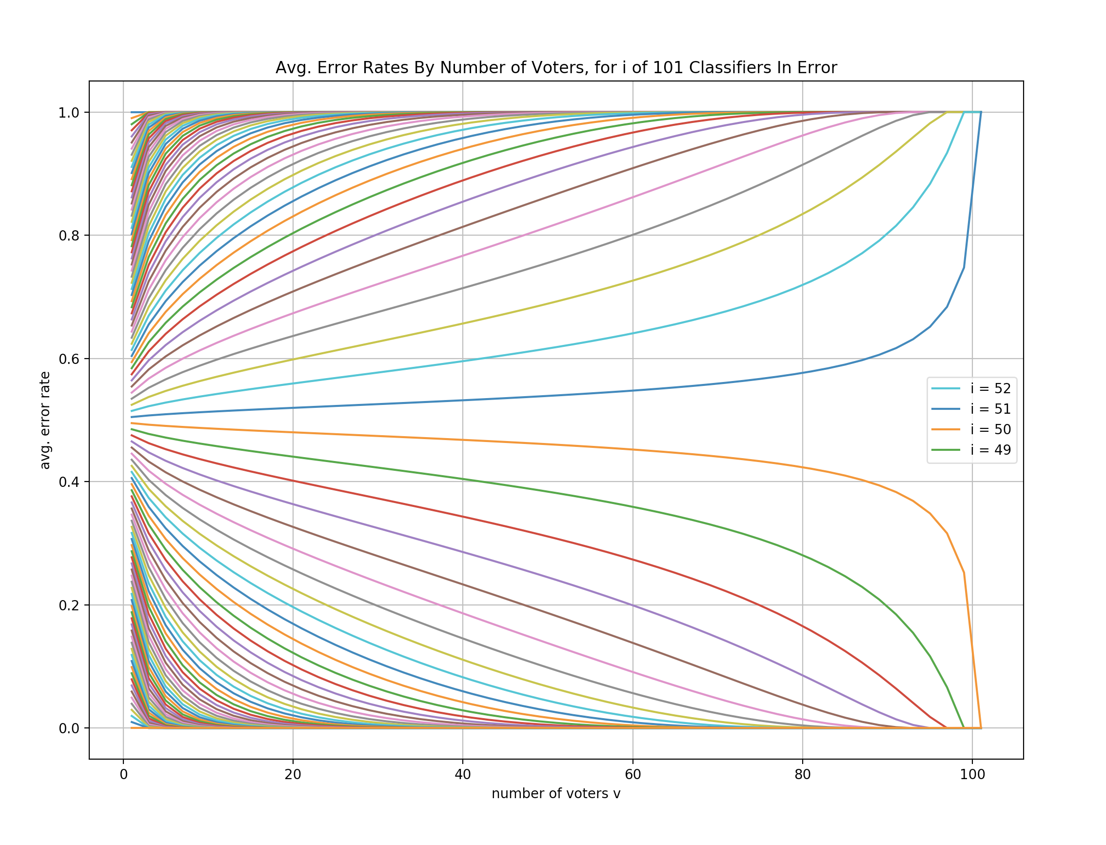
Figure 1: Average error rates $r(m,i,v)$, for $v$ voters, if $i\in\left\{{0,\ldots,101}\right\}$ of $m=101$ classifiers are incorrect. The line for $i=0$ is at the bottom of the figure – a flat line of average error rate zero, since if all classifiers are correct, then any number of voters gives correct classification. Similarly, the line for $i=101$ is at the top, and successive curves are for successive $i$-values. (Only the middle four are labeled, to avoid cluttering the figure.).

Figure 1 shows how the probability of error for a voting classifier, $r(m,i,v)$ varies with the number of voters $v$, given that $i$ of $m$ classifiers are in error. The plot is for $m=101$, with a curve for each number of errors $i\in\left\{{0,\ldots,101}\right\}$, connecting $r(m,i,v)$ values for odd $v$ from one to 101. Think of the curves as a basis. The set of weighted averages of the curves is the set of all possible error curves with respect to number of voters $v$ for ensembles of $m=101$ classifiers.

From Figure 1, notice that if more than half the classifiers are in error ($i\geq 51$), then using more voters increases the out-of-sample error rate (except for $i=101$ since it always gives a 100% error rate). To see why consider $i=51$. If 51 of 101 classifiers are in error, then selecting a single one and using it gives expected error rate $\frac{51}{101}$, but using all $101$ always results in an error, because 51 is a (slight) majority of the 101 voters. Between 1 and 101, using more voters increases the error rate, by making it more likely that the majority of voters will be incorrect. Also, notice that as $i$ increases above 51, the increase in error rate with number of voters goes from concave up to nearly linear to concave down, showing that the loss in accuracy due to using a few voters rather than a single classifier increases with $i$.

The following theorem shows that some things we can observe in Figure 1 are true in general: adding voters strengthens classification for examples with fewer than half the ensemble classifiers in error, and it weakens classification for examples with more than half the ensemble classifiers in error. These effects only cease when there are so many voters that the minority among the ensemble (correct or incorrect) is too small to be a majority of the voters.

Theorem 3.

Let $r(m,i,v)$ be the voting ensemble error rate if $i$ of $m$ ensemble classifiers are in error, $v$ voters are selected at random without replacement from the ensemble, and their majority vote is returned. (Assume $v$ is odd.) Define the error rate difference due to increasing the number of voters by two:

$$\Delta_{v}(m,i,v)\equiv r(m,i,v+2)-r(m,i,v).$$ (9)

Then:

• If $i<\frac{v+1}{2}$ then $r(m,i,v)=0$ and $\Delta_{v}(m,i,v)=0$.

• If $i<\frac{m}{2}$ and $i\geq\frac{v+1}{2}$, then $\Delta_{v}(m,i,v)<0$.

• If $i>\frac{m}{2}$ and $m-i\geq\frac{v+1}{2}$, then $\Delta_{v}(m,i,v)>0$.

• If $m-i<\frac{v+1}{2}$ then $r(m,i,v)=1$ and $\Delta_{v}(m,i,v)=0$.

Proof.

The first and last bullet points in the theorem are straightforward. For the others, suppose $v$ voters have been selected from $m$ classifiers. How can adding two voters make an incorrect decision correct? There is only one way: the $v$ voters must contain the maximum number of incorrect voters to still be correct: $\frac{v-1}{2}$, and both added voters must be incorrect. That makes the number of incorrect voters

$$\frac{v-1}{2}+2=\frac{v+3}{2}=\frac{(v+2)+1}{2},$$ (10)

out of $v+2$ voters. Since this is the minimum possible majority, starting with fewer than $\frac{v-1}{2}$ incorrect voters or adding fewer than two incorrect voters will not work. Similarly, to go from incorrect with $v$ voters to correct with $v+2$ voters, it is necessary to start with $\frac{v+1}{2}$ incorrect voters and add two correct voters.

Note that $\Delta_{v}(m,i,v)$ is the difference between the probability of going from correct to incorrect and the probability of going from incorrect to correct. The probability of going from incorrect to correct is the probability of selecting $\frac{v-1}{2}$ of the $i$ incorrect voters when selecting $v$ of the $m$ classifiers without replacement, times the probability of getting two incorrect classifiers when selecting two of the remaining $m-v$ classifiers as voters:

$$\frac{{{i}\choose{\frac{v-1}{2}}}{{m-i}\choose{\frac{v+1}{2}}}}{{{m}\choose{v}}}\left(\frac{i-\frac{v-1}{2}}{m-v}\right)\left(\frac{i-\frac{v-1}{2}-1}{m-v-1}\right).$$ (11)

Similarly, the probability of going from incorrect to correct is:

$$\frac{{{i}\choose{\frac{v+1}{2}}}{{m-i}\choose{\frac{v-1}{2}}}}{{{m}\choose{v}}}\left(\frac{m-i-\frac{v-1}{2}}{m-v}\right)\left(\frac{m-i-\frac{v-1}{2}-1}{m-v-1}\right).$$ (12)

To find the difference, $\Delta_{v}(m,i,v)$, note that

$${{i}\choose{\frac{v-1}{2}}}=\frac{i(i-1)!}{\left(\frac{v-1}{2}\right)!\left(i-\frac{v-1}{2}\right)\left(i-1-\frac{v-1}{2}\right)!}$$ (13)

$$=i{{i-1}\choose{\frac{v-1}{2}}}\left(\frac{1}{i-\frac{v-1}{2}}\right),$$ (14)

and

$${{i}\choose{\frac{v+1}{2}}}=\frac{i(i-1)!}{\left(\frac{v+1}{2}\right)\left(\frac{v-1}{2}\right)!\left(i-\frac{v+1}{2}\right)!}$$ (15)

$$=\frac{i(i-1)!}{\left(\frac{v+1}{2}\right)\left(\frac{v-1}{2}\right)!\left(i-1-\frac{v-1}{2}\right)!}$$ (16)

$$=i{{i-1}\choose{\frac{v-1}{2}}}\left(\frac{1}{\frac{v+1}{2}}\right).$$ (17)

Similarly,

$${{m-i}\choose{\frac{v+1}{2}}}=\left(m-i\right){{m-i-1}\choose{\frac{v-1}{2}}}\left(\frac{1}{\frac{v+1}{2}}\right),$$ (18)

and

$${{m-i}\choose{\frac{v-1}{2}}}=\left(m-i\right){{m-i-1}\choose{\frac{v-1}{2}}}\left(\frac{1}{m-i-\frac{v-1}{2}}\right).$$ (19)

Use these equalities to factor out some common terms:

$$\Delta_{v}(m,i,v)={{m}\choose{v}}^{-1}i{{i-1}\choose{\frac{v-1}{2}}}\left(m-i\right){{m-i-1}\choose{\frac{v-1}{2}}}$$ (20)

$$\left[\frac{\left(\frac{i-\frac{v-1}{2}}{m-v}\right)\left(\frac{i-\frac{v-1}{2}-1}{m-v-1}\right)}{\left(i-\frac{v-1}{2}\right)\left(\frac{v+1}{2}\right)}\right.$$ (21)

$$\left.-\frac{\left(\frac{m-i-\frac{v-1}{2}}{m-v}\right)\left(\frac{m-i-\frac{v-1}{2}-1}{m-v-1}\right)}{\left(\frac{v+1}{2}\right)\left(m-i-\frac{v-1}{2}\right)}\right].$$ (22)

For both terms in brackets, cancel one denominator factor with a numerator factor, and factor out the other denominator factors:

$$\Delta_{v}(m,i,v)={{m}\choose{v}}^{-1}i{{i-1}\choose{\frac{v-1}{2}}}\left(m-i\right){{m-i-1}\choose{\frac{v-1}{2}}}$$ (23)

$$\frac{\left[\left(i-\frac{v-1}{2}-1\right)-\left(m-i-\frac{v-1}{2}-1\right)\right]}{\left(\frac{v+1}{2}\right)\left(m-v\right)\left(m-v-1\right)}.$$ (24)

Then cancel in brackets:

$$\Delta_{v}(m,i,v)={{m}\choose{v}}^{-1}i{{i-1}\choose{\frac{v-1}{2}}}\left(m-i\right){{m-i-1}\choose{\frac{v-1}{2}}}$$ (25)

$$\frac{\left[2i-m\right]}{\left(\frac{v+1}{2}\right)\left(m-v\right)\left(m-v-1\right)}.$$ (26)

Only the term $2i-m$ may be negative. It is negative if $i<\frac{m}{2}$ and positive if $i>\frac{m}{2}$. Based on the second through fifth factors, $\Delta_{v}(m,i,v)=0$ if at least one of the following conditions holds: $i=0$, $i=m$, $i-1<\frac{v-1}{2}$ (equivalently: $i<\frac{v+1}{2}$), or $m-i<\frac{v+1}{2}$. ∎

4 Optimal numbers of voters

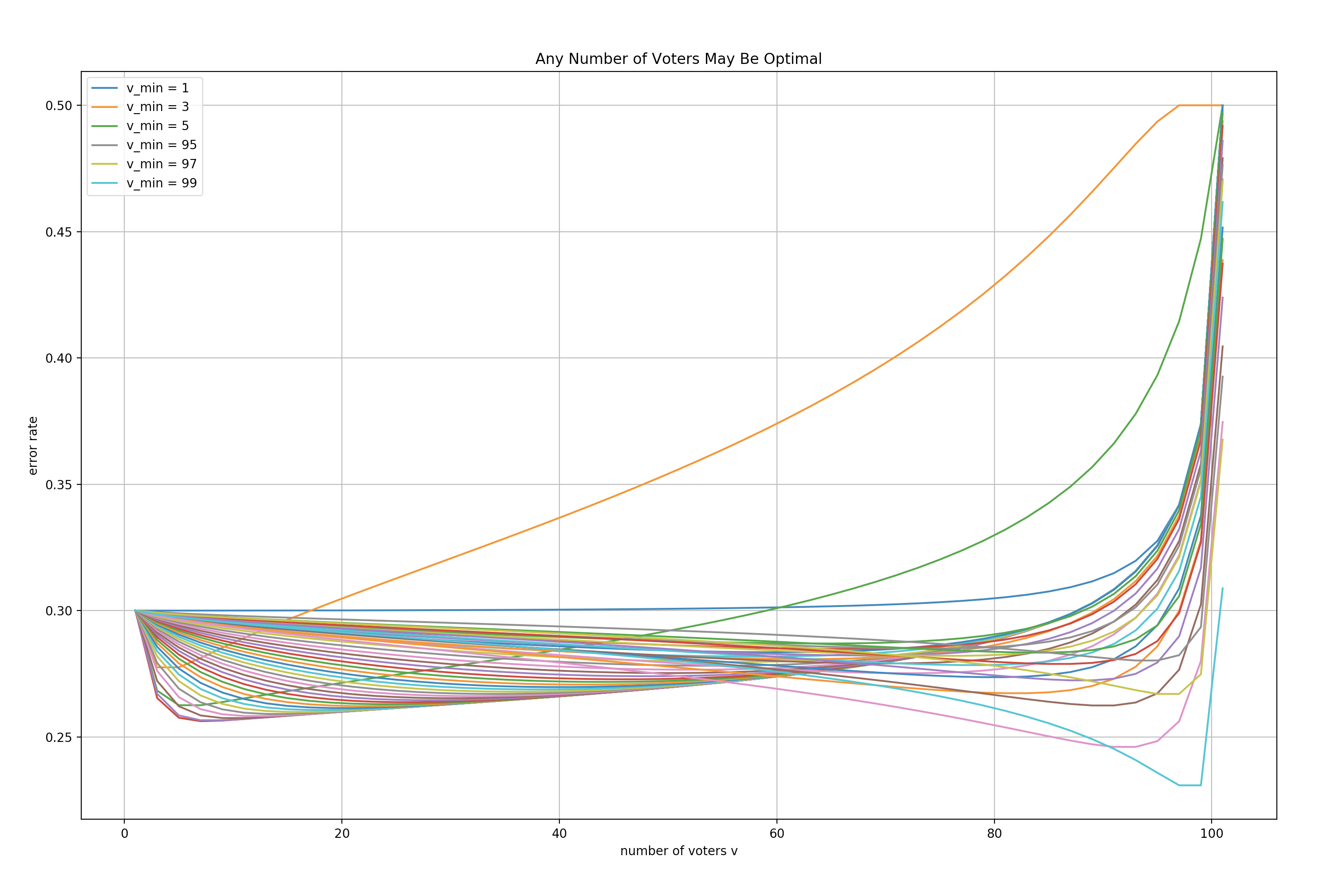
Figure 2: Any (odd) number of voters may be optimal. For $m=101$, error curves for which each $v_{*}\in\left\{{1,3,\ldots,99}\right\}$ is an error-minimizing number of voters. (Each curve is based on a different distribution over number of ensemble classifiers incorrect. Average ensemble classifier error rate is 0.3.)

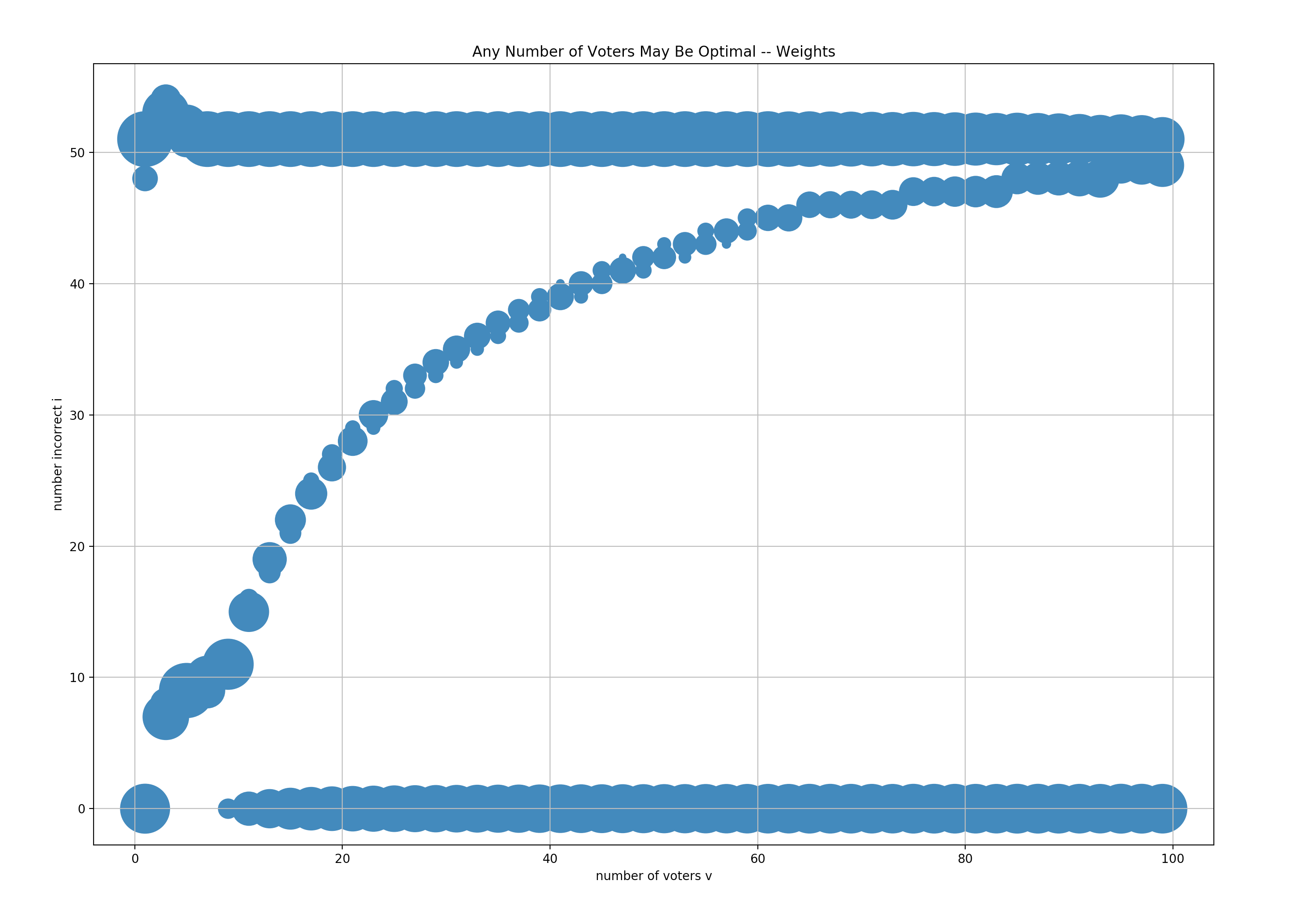
Figure 3: Distributions $w_{i}$ for $i\in\left\{{0,\ldots,101}\right\}$ that produce curves for which $v=v_{*}$ is an error-minimizing number of voters.

Any (odd) number of voters may be optimal. For each $v_{*}\in\left\{{1,3,\ldots,99}\right\}$, with $m=101$, Figure 2 shows a voting error rate curve for a distribution $(w_{0},\ldots,w_{m})$ for which $v_{*}$ is an error-minimizing number of voters. For each curve, the distribution $(w_{0},\ldots,w_{m})$ is produced by a linear program that maximizes difference in error rates between using 101 and using $v_{*}$ voters, subject to constraints:

• voting error rate with $v_{*}$ classifiers is no more than that for a single voter, for $v_{*}-2$ voters, or for $v_{*}+2$ voters,

• voting error rate with all classifiers voting is at most $0.5$ (otherwise, it is possible to just use the opposite of its output to get a lower error rate), and

• average error rate over classifiers is 0.3.

The figure shows that any odd number of voters up to 99 can minimize error rate for $m=101$. The figure does not show this for $v_{*}=101$, since the linear program optimizes the difference between using $v_{*}$ and using 101 voters. However, Figure 1 shows that 101 is the optimal number of voters for the distribution $w_{50}=1$ and all other $w_{i}=0$.

Figure 3 shows the distributions of weights for each $v_{*}$ curve in Figure 2. For most $v_{*}$ values, the error count distributions $(w_{0},\ldots,w_{m})$ that give the largest gap between using $v_{*}$ voters and the full set of $m=101$ voters have some weight on $w_{0}$, some on $w_{51}$, and some on one or two intermediate numbers of errors. The curve for each $v_{*}$ is the weighted sum of the ”basis” curves for $i=0$, $i=51$, and the intermediate value or values from Figure 1. The weight on $w_{0}$ lowers error rates, helping enforce the constraint on average error rate over classifiers and the constraint on error rate for 101 voters. The weight on $w_{51}$ ensures that the curve for $v_{*}$ goes up on the right, increasing the difference in error rates between $v_{*}$ voters and 101 voters as well as helping to ensure that $v_{*}$ voters is locally optimal compared to $v_{*}+2$ voters. Any weights on intermediate values can contribute to the curvature, ensuring that $v_{*}$ voters is locally optimal compared to $v_{*}-2$ voters. These weights can give us insight into how to prove that any (odd) number of voters can be optimal for any number $m$ of classifiers:

Theorem 4.

For $m>0$ and any $v_{*}\in\left\{{1,3,\ldots,m}\right\}$, there is a distribution $(w_{0},\ldots,w_{m})$, where $w_{i}$ is the probability that $i$ of $m$ classifiers are in error, such that $v_{*}$ voters achieves the minimum voting error rate.

Proof.

First consider the boundary cases: $v_{*}=1$ and $v_{*}=m$ (or $v_{*}=m-1$ if $m$ is even). If $v_{*}=1$, then set $w_{m-1}=1$. That gives a $\frac{m-1}{m}$ error rate for $v=1$, since there is one correct classifier, and error rate one for $v\geq 3$, since the single correct classifier cannot form a majority. Similarly, if $v_{*}=m$ or $v_{*}=m-1$, then set $w_{i}=1$ for $i=\frac{v_{*}-1}{2}$. That produces error rate zero for $v_{*}$ voters, because the incorrect voters cannot form a majority, but the error rate for smaller $v$ values is positive since the incorrect voters can form a majority for those values.

Now consider intermediate values: $1<v_{*}<m-1$. Let $a=\frac{v_{*}-1}{2}$ and $b=m-\frac{v_{*}+1}{2}$. For $a$ errors among $m$ classifiers, the voting error rate is zero for $v\geq v_{*}$. For $b$ errors, it is one for $v>v_{*}$, but less than one for $v=v_{*}$, because the $\frac{v_{*}+1}{2}$ can form a majority among $v_{*}$ voters. As a result, any weighted average (with positive weights) of error curves for $a$ and $b$ has voting error rate greater than $v_{*}$ for all $v>v_{*}$. So set $w_{a}=\theta$, $w_{b}=1-\theta$, and $w_{i}=0$ for all other $i$ values.

Then select $\theta\in(0,1)$ to ensure that the linear combination of curves has voting error rates less than the rate for $v_{*}$ for all $v<v_{*}$. It is possible to do this by taking $\theta$ sufficiently close to one, because doing so makes the combined curve resemble the curve for $a$ errors more and the curve for $b$ errors less. (This requires that the error rates on the curve for $b$ be bounded, so that multiplying by $1-\theta$ can reduce their influence as $1-\theta$ approaches zero, but they are bounded by one since they are error rates.) By Theorem 3, the curve for $a$ errors is strictly decreasing in $v$ for $v<v_{*}$, since $i=a=\frac{v_{*}-1}{2}<\frac{m}{2}$ and $i=a=\frac{v_{*}-1}{2}\geq\frac{v+1}{2}$. ∎

5 Selecting the number of voters

Assume we have $n$ validation examples, drawn i.i.d. from the out-of-sample distribution, and not used to train or select classifiers for the ensemble, and we want to use them to select the number of voters for the ensemble. A straightforward method is to apply the voting classifier for each odd number of voters $v$ in one to $m$ to all the validation examples, selecting voters at random for each number of voters and validation example. Then calculate the error rate over the validation examples for each number of voters, and select the number of voters with the lowest validation error rate.

To get error bounds, for each number of voters $v$, let $k_{v}$ be the number of errors over the validation examples. Let $u(n,k,\delta)$ be a PAC (probably approximately correct) upper bound and $t(n,k,\delta)$ be a PAC lower bound for the probability that produces $k$ events in $n$ samples with bound failure probability $\delta$. Since we simultaneously validate error rates for $\frac{m+1}{2}$ different numbers of voters and use two-sided bounds, for $\delta>0$, with probability at least $1-\delta$, each number of voters has out-of-sample distribution error rate in the range $t(n,k_{v},\frac{\delta}{m+1})$ to $u(n,k_{v},\frac{\delta}{m+1})$. For example, using Hoeffding bounds (Hoeffding, 1963), the range is:

$$\frac{k_{v}}{n}\pm\sqrt{\frac{\ln(m+1)-\ln\delta}{2n}}.$$ (27)

In practice, use a binomial inversion bound (Hoel, 1954; Langford, 2005), to get a tighter bound range.

Selecting voters at random for each example introduces some variance. To produce lower-variance estimates of voting error rates, instead compute for each validation example $j$ the number of ensemble classifiers in error $i_{j}$. Recall from Equation 5 that $r(m,i,v)$ is the expected voting error rate for $v$ voters, given $i$ ensemble classifiers in error. Then, for each number of voters $v$, an estimate of out-of-sample error rate is:

$$\frac{1}{n}\sum_{j=1}^{n}r(m,i_{j},v).$$ (28)

Let $\hat{w}_{i}$ be the fraction of validation examples for which there are $i$ classifiers in error ($i_{j}=i$). Then the estimate is

$$=\sum_{i=0}^{m}\hat{w}_{i}r(m,i,v).$$ (29)

Refer to these estimates as the inference estimates, since they use estimates of the rates of numbers of errors in the ensemble to infer a estimates of out-of-sample error rates for different numbers of voters.

Theorem 5.

For each number of voters $v$, the out-of-sample error rate estimate from using validation data to compute estimates $\hat{w}_{i}$ and using them to infer average voting error rate has variance less than or equal to the estimate from applying randomly-selected voters to validation examples.

Proof.

For inference, the estimate is the mean of $r(m,i,v)$ over validation examples, where $i$ is the number of ensemble classifiers in error. For brevity, call $r(m,i,v)$ simply $r_{i}$. The direct estimate is the mean over validation examples of one if voting errs and zero otherwise. For both, the variance sums over examples, since the validation examples are independent samples. So we can focus on the variances for a single validation example.

For direct estimation, the single-example error estimate is one with probability $p$, where $p$ is the out-of-sample distribution error rate for using $v$ voters, and zero with probability $1-p$. Since it is a Bernoulli random variable, it has variance $p(1-p)=p-p^{2}$.

For inference, the single-example error estimate is $r(m,i,v)$, with probability $w_{i}$ for each value of $i$. The variance is the difference between the expectation of the square and the square of the expectation:

$$\sum_{i}w_{i}r_{i}^{2}-\left[\sum_{i}w_{i}r_{i}\right]^{2}.$$ (30)

But

$$p=\sum_{i}w_{i}r_{i},$$ (31)

so the variance is

$$\sum_{i}w_{i}r_{i}^{2}-p^{2}.$$ (32)

Recall that the variance for direct estimation is $p-p^{2}$. So the difference between variances is

$$p-\sum_{i}w_{i}r_{i}^{2}=\sum_{i}w_{i}r_{i}-\sum_{i}w_{i}r_{i}^{2}=\sum_{i}w_{i}\left[r_{i}-r_{i}^{2}\right].$$ (33)

Since each $r_{i}$ is a probability (of voting error given $i$ ensemble errors), $r_{i}\in[0,1]$. So $r_{i}^{2}\leq r_{i}$. ∎

6 Error Bounds and Inference

6.1 Error Bounds

Now consider how to compute error bounds based on the inference estimates. One way is to apply simultaneous Hoeffding bounds:

Theorem 6.

With probability at least $1-\delta$, the out-of-sample error rates for all numbers of voters $v$ are within

$$\sqrt{\frac{\ln(m+1)-\ln\delta}{2n}}$$ (34)

of the inference estimates from Expressions 28 and 29.

Proof.

From Expression 28, the inference estimate for each $v$ is

$$\frac{1}{n}\sum_{j=1}^{n}r(m,i_{j},v).$$ (35)

This is the average of $n$ i.i.d. random variables $r(m,i_{j},v)\in[0,1]$, one for each validation example $j$. The estimate’s mean (over draws of validation examples) is the out-of-sample error rate for $v$, since $r(m,i,v)$ is the average error rate for $v$ voters, averaged over all sets of $v$ voters. So Hoeffding bounds apply (Hoeffding, 1963). There are $\frac{m+1}{2}$ numbers of voters, and two-sided bounds, making $m+1$ simultaneous validations. So set $\delta$ to $\frac{\delta}{m+1}$ in the Hoeffding bound. ∎

6.2 Validation by Inference

Alternatively, we could first bound out-of-sample rates of $i$ errors among the ensemble classifiers, then use those bounds to infer bounds on ensemble error rates. (This strategy is called validation by inference (Bax, 2000).) As before, let $w_{i}$ be the out-of-sample rate of $i$ errors among the $m$ ensemble classifiers, and let $\hat{w}_{i}$ be the in-sample rate over $n$ validation examples. Also as before, let $u(n,k,\delta)$ and $t(n,k,\delta)$ be PAC upper and lower bounds on the out-of-sample probability that produces $k$ events in $n$ samples, with bound failure probability $\delta$.

Then, using simultaneous validation for $2(m+1)$ bounds (2 for upper and lower bounds, and $m+1$ for zero to $m$ errors among the ensemble classifiers), with probability at least $1-\delta$,

$$\forall_{i\in\{1,\ldots,m\}}w_{i}\in\left[t(n,\hat{w}_{i}n,\frac{\delta}{2(m+1)}),u(n,\hat{w}_{i}n,\frac{\delta}{2(m+1)})\right].$$ (36)

(Dividing $\delta$ to get simultaneous bounds is known as the Bonferroni correction (Bonferroni, 1936; Dunn, 1961).)

To derive out-of-sample error bounds for each number of voters $v$, use linear programming to optimize

$$\sum_{i=0}^{m}w_{i}r(m,i,v)$$ (37)

over the set of feasible out-of-sample rates of numbers of errors given by Expression 36, with the additional constraints

$$\sum_{i=0}^{m}w_{i}=1\hbox{ and }\forall i:w_{i}\geq 0,$$ (38)

minimizing for lower bounds and maximizing for upper bounds.

Compare these bounds to the bounds from Theorem 6. These bounds allow binomial inversion for each $t_{i}$ and $u_{i}$, since each $\hat{w}_{i}$ has a binomial distribution, and these tend to be tighter than Hoeffding bounds and other derived bounds. (Binomial inversion gives sharp bounds.) However, these bounds divide $\delta$ by $2(m+1)$ rather than $m+1$, doubling the bound failure probability allocated to each probability bound, because we use $m+1$ estimated rates of numbers of errors among classifiers to infer error bounds for only $\frac{m+1}{2}$ numbers of voters $v$.

6.3 Using the Multinomial Distribution – Future Work

Together, the $\hat{w}_{i}$ values are a sample from a multinomial distribution with probabilities $w_{i}$. We should be able to use this information to get tighter bounds on the $w_{i}$ values from multinomial bounds, instead of using simultaneous binomial bounds over all $\hat{w}_{i}$. Let $L(\mathbf{\hat{w}},\delta)$ be the set of probability vectors $\mathbf{w}=(w_{0},\ldots,w_{m})$ that have probability at least $1-\delta$ of generating a sample vector that is more likely than $\mathbf{\hat{w}}=(\hat{w}_{0},\ldots,\hat{w}_{m})$. Call $L(\mathbf{\hat{w}},\delta)$ the likely set. (Informally, $\mathbf{w}$ is in the likely set unless $\mathbf{\hat{w}}$ is in the $\delta$-tail of the multinomial distribution generated by probabilities $\mathbf{w}$.)

To compute an upper bound on out-of-sample error rate for each number of voters $v$, solve:

$$\max_{\mathbf{w}\in L(\mathbf{\hat{w}},\delta)}\sum_{i=0}^{m}w_{i}r(m,i,v).$$ (39)

(For lower bounds, minimize instead of maximizing.) This produces valid upper and lower bounds for all numbers of voters, with probability at least $1-\delta$.

Constraining $\mathbf{w}$ to the likely set based on the multinomial distribution allows validation by inference without using a Bonferroni correction to divide $\delta$ by $2(m+1)$ as was required for the constraints in Expression 36. This produces tighter constraints, so the resulting bounds are at least as strong.

The challenge lies in computing the error bounds. We want to optimize a linear function over the likely set. But the likely set may have a challenging shape for optimization, because the tails of multinomial distributions are not continuous in $\mathbf{w}$. To see why, suppose that for some $\mathbf{w}$ some other sample vector is equally as likely as $\mathbf{\hat{w}}$. Then perturbing $\mathbf{w}$ can change the ordering of those likelihoods, so that the likelihood of the other sample vector becomes greater than that of $\mathbf{\hat{w}}$, shifting the other sample vector’s full probability out of the tail in a discontinuous jump.

So one goal for future research is to identify a superset of the likely set that is amenable to optimization and does not contain distributions $\mathbf{w}$ outside the likely set that would significantly weaken the resulting error bounds. There are approximations to the likely set that make optimization easier. For example, consider Pearson’s $X^{2}$ statistic (Pearson, 1900; Read and Cressie, 1988; Cressie and Read, 1984):

$$X^{2}(\mathbf{w},\mathbf{\hat{w}})=(m+1)\sum_{i=0}^{m}\frac{(\hat{w}_{i}-w_{i})^{2}}{w_{i}},$$ (40)

with term $i$ zero if $w_{i}=\hat{w}_{i}=0$. Asymptotically, $X^{2}$ has a chi-squared distribution with $m$ degrees of freedom. So if we let $C_{\delta}$ be the value for which the cdf of that distribution is $\delta$, then we can define an approximate likely set:

$$\tilde{L}(\mathbf{\hat{w}},\delta)\equiv\left\{\mathbf{w}\left|X^{2}(\mathbf{w},\mathbf{\hat{w}})\leq C_{\delta}\right.\right\}.$$ (41)

This set has smooth boundaries. However, it is not a superset of the likely set.

To identify a suitable superset of the likely set, perhaps we can apply bounds on the difference between $X^{2}$ (or similar statistics) and the chi-squared distribution (Matsunawa, 1977; Siotani and Fujikoshi, 1984; Bickel and Ghosh, 1990; Taneichi et al., 2002; Gaunt et al., 2016; Ouimet, 2021) to expand an approximate likely set, for example by increasing the constraint $C_{\delta}$ on $X^{2}$ to ensure that all $\mathbf{w}$ in the likely set are enclosed in the region of the approximate set while keeping the set small enough to yield effective error bounds. It may also be possible to extend bounds on $L_{1}$ distance between $\mathbf{\hat{w}}$ and $\mathbf{w}$ (Valiant and Valiant, 2017; Balakrishnan and Wasserman, 2018) to derive a superset of the likely set that gives linear constraints instead of a feasible region with curved boundaries.

Within optimization procedures, computing tail probabilities (the cdf of $\mathbf{\hat{w}}$ given $\mathbf{w}$) directly is infeasible for even moderate-sized ensembles, because the number of ways for $n$ samples to fall into $m+1$ categories is ${n+m}\choose{m}$. Monte Carlo methods (Hope, 1968; Jann, 2008) can estimate the tail probability to arbitrary accuracy with arbitrarily high probability. Also, there are evolving methods to cleverly collect terms for exact tail computation (Baglivo et al., 1992; Keich and Nagarajan, 2006; Resin, 2020).

The problem of identifying a worst likely generator for multinomial samples is an interesting statistical problem, with applications beyond ensemble validation. It is not clear whether approaches based on the multinomial tail can be more effective in practice than approaches that split $\delta$ and perform simultaneous validation over individual categories. (In our case, each number of errors $i$ among the ensemble classifiers is a category.) The simpler approach of simultaneous validation can use sharp binomial inversion bounds within each category, and it can also benefit from the freedom to split $\delta$ non-uniformly. Finally, both approaches could benefit from tuning the constraints to the weights (the $r(m,i,v)$ values in our case) used to evaluate the generating distributions. For example, it is possible to merge categories that have similar weights to reduce the problem’s dimensionality.

References

- Baglivo et al. (1992) Baglivo, J., Olivier, D., Pagano, M., 1992. Methods for exact goodness-of-fit tests. Journal of the American Statistical Association 87, 464–469. doi:10.1080/01621459.1992.10475227.
- Balakrishnan and Wasserman (2018) Balakrishnan, S., Wasserman, L., 2018. Hypothesis testing for high-dimensional multinomials: A selective review. The Annals of Applied Statistics 12, 727 – 749. URL: https://doi.org/10.1214/18-AOAS1155SF, doi:10.1214/18-AOAS1155SF.
- Bax (1998) Bax, E., 1998. Validation of voting committees. Neural Computation 10, 975–986. URL: https://doi.org/10.1162/089976698300017584, doi:10.1162/089976698300017584.
- Bax (2000) Bax, E., 2000. Using validation by inference to select a hypothesis function, in: Pattern Recognition, International Conference on, IEEE Computer Society, Los Alamitos, CA, USA. p. 2700. URL: https://doi.ieeecomputersociety.org/10.1109/ICPR.2000.906171, doi:10.1109/ICPR.2000.906171.
- Begin et al. (2016) Begin, L., Germain, P., Laviolette, F., Roy, J.F., 2016. Pac-bayesian bounds based on the renyi divergence. Proceedings of the 19th International Conference on Artificial Intelligence and Statistics (AISTATS) .
- Bennett and Lanning (2007) Bennett, J., Lanning, S., 2007. The netflix prize. Proceedings of the KDD Cup Workshop , 3–6.
- Bickel and Ghosh (1990) Bickel, P.J., Ghosh, J.K., 1990. A Decomposition for the Likelihood Ratio Statistic and the Bartlett Correction–A Bayesian Argument. The Annals of Statistics 18, 1070 – 1090. URL: https://doi.org/10.1214/aos/1176347740, doi:10.1214/aos/1176347740.
- Bonab and Can (2019) Bonab, H., Can, F., 2019. Less is more: A comprehensive framework for the number of components of ensemble classifiers. IEEE Transactions on Neural Networks and Learning Systems 30, 2735–2745.
- Bonferroni (1936) Bonferroni, C.E., 1936. Teoria statistica delle classi e calcolo delle probabilità .
- Breiman (1996) Breiman, L., 1996. Bagging predictors. Machine Learning 24, 123–140.
- Breiman (2001) Breiman, L., 2001. Random forests. Machine Learning 45, 5–32.
- Chen and Guestrin (2016) Chen, T., Guestrin, C., 2016. Xgboost: A scalable tree boosting system. KDD ’16: Proceedings of the 22nd ACM SIGKDD International Conference on Knowledge Discovery and Data Mining , 785–794URL: https://arxiv.org/pdf/1603.02754v1.pdf.
- Cressie and Read (1984) Cressie, N., Read, T.R.C., 1984. Multinomial goodness-of-fit tests. J. R. Statist. Soc. B 46, 440–464.
- Dietterich (2000) Dietterich, T.G., 2000. Ensemble methods in machine learning, in: Multiple Classifier Systems, Springer Berlin Heidelberg, Berlin, Heidelberg. pp. 1–15.
- Dunn (1961) Dunn, O.J., 1961. Multiple comparisons among means. Journal of the American Statistical Association 56, 52–64. URL: https://www.tandfonline.com/doi/abs/10.1080/01621459.1961.10482090, doi:10.1080/01621459.1961.10482090.
- Esposito and Saitta (2004) Esposito, R., Saitta, L., 2004. A monte carlo analysis of ensemble classification. doi:10.1145/1015330.1015386.
- Freund and Schapire (1997) Freund, Y., Schapire, R., 1997. A decision-theoretic generalization of on-line learning and an application to boosting. System Sciences 55, 119–139.
- Gaunt et al. (2016) Gaunt, R.E., Pickett, A., Reinert, G., 2016. Chi-square approximation by Stein’s method with application to Pearson’s statistic. arxiv URL: https://arxiv.org/pdf/1507.01707.pdf.
- Gomes et al. (2017) Gomes, H.M., Barddal, J.P., Enembreck, F., Bifet, A., 2017. A survey on ensemble learning for data stream classification. ACM Comput. Surv. 50. URL: https://doi.org/10.1145/3054925, doi:10.1145/3054925.
- Hernández-Lobato et al. (2013) Hernández-Lobato, D., Martínez-Muñoz, G., Suárez, A., 2013. How large should ensembles of classifiers be? Pattern Recognition 46, 1323 – 1336. URL: http://www.sciencedirect.com/science/article/pii/S0031320312004554, doi:https://doi.org/10.1016/j.patcog.2012.10.021.
- Ho (1995) Ho, T.K., 1995. Random decision forests. Proceedings of the 3rd International Conference on Document Analysis and Recognition, Montreal, QC , 278–282.
- Ho (1998) Ho, T.K., 1998. The random subspace method for constructing decision forests. EEE Transactions on Pattern Analysis and Machine Intelligence 20, 832–844.
- Hoeffding (1963) Hoeffding, W., 1963. Probability inequalities for sums of bounded random variables. Journal of the American Statistical Association 58, 13–30.
- Hoel (1954) Hoel, P.G., 1954. Introduction to Mathematical Statistics. Wiley.
- Hope (1968) Hope, A.C.A., 1968. A simplified Monte Carlo significance test procedure. Journal of the Royal Statistical Society. Series B 30, 582–598.
- Hu (2001) Hu, X., 2001. Using rough sets theory and database operations to construct a good ensemble of classifiers for data mining applications. Proc. IEEE Int. Conf. Data Mining (ICDM) , 233–240.
- Jackowski (2018) Jackowski, K., 2018. New diversity measures for data stream classification ensembles 74, 23–34.
- Jann (2008) Jann, B., 2008. Multinomial goodness-of-fit: Large-sample tests with survey design correction and exact tests for small samples. The Stata Journal 8, 147–169. URL: https://doi.org/10.1177/1536867X0800800201, doi:10.1177/1536867X0800800201, arXiv:https://doi.org/10.1177/1536867X0800800201.
- Keich and Nagarajan (2006) Keich, U., Nagarajan, N., 2006. A fast and numerically robust method for exact multinomial goodness-of-fit test. Journal of Computational and Graphical Statistics 15, 779--802. URL: https://doi.org/10.1198/106186006X159377, doi:10.1198/106186006X159377.
- Kuncheva (2004) Kuncheva, L.I., 2004. Combining Pattern Classifiers: Methods and Algorithms. Wiley.
- Kuncheva et al. (2003) Kuncheva, L.I., Whitaker, C.J., Shipp, C.A., Duin, R.P.W., 2003. Limits on the majority vote accuracy in classifier fusion. Pattern Analysis & Applications 6, 22--31. URL: https://doi.org/10.1007/s10044-002-0173-7, doi:10.1007/s10044-002-0173-7.
- Lam and Suen (1997) Lam, L., Suen, S.Y., 1997. Application of majority voting to pattern recognition: an analysis of its behavior and performance. IEEE Transactions on Systems, Man, and Cybernetics - Part A: Systems and Humans 27, 553--568.
- Langford (2005) Langford, J., 2005. Tutorial on practical prediction theory for classification. Journal of Machine Learning Research 6, 273--306.
- Langford et al. (2001) Langford, J., Seeger, M., Megiddo, N., 2001. An improved predictive accuracy bound for averaging classifiers, in: In Proceeding of the Eighteenth International Conference on Machine Learning, pp. 290--297.
- Li (2010) Li, P., 2010. Robust logitboost and adaptive base class (abc) logitboost. Proceedings of the Twenty-Sixth Conference Annual Conference on Uncertainty in Artificial Intelligence (UAI’10) , 302–311.
- Liu et al. (2004) Liu, H., Mandvikar, A., Mody, J., 2004. An empirical study of building compact ensembles. Web-Age Information Management (WAIM) , 622--627.
- Matsunawa (1977) Matsunawa, T., 1977. Approximations to the probabilities of binomial and multinomial random variables and chi-square type statistics. Annals of the Institute of Statistical Mathematics 29, 333. URL: https://doi.org/10.1007/BF02532796, doi:10.1007/BF02532796.
- McAllester (1999) McAllester, D.A., 1999. Pac-bayesian model averaging, in: In Proceedings of the Twelfth Annual Conference on Computational Learning Theory, ACM Press. pp. 164--170.
- Oshiro et al. (2012) Oshiro, T.M., Perez, P.S., Baranauskas, J.A., 2012. How many trees in a random forest?, in: Perner, P. (Ed.), Machine Learning and Data Mining in Pattern Recognition, Springer Berlin Heidelberg, Berlin, Heidelberg. pp. 154--168.
- Ouimet (2021) Ouimet, F., 2021. A precise local limit theorem for the multinomial distribution and some applications. Journal of Statistical Planning and Inference 215, 218--233. URL: https://www.sciencedirect.com/science/article/pii/S0378375821000392, doi:https://doi.org/10.1016/j.jspi.2021.03.006.
- Pearson (1900) Pearson, K., 1900. On the criterion that a given system of deviations from the probable in the case of a correlated system of variables is such that it can be reasonably supposed to have arisen from random sampling. Philosophical Magazine. Series 5 302, 157--175.
- Read and Cressie (1988) Read, T.R.C., Cressie, N.A.C., 1988. Goodness-of-fit statistics for discrete multivariate data. New York: Springer-Verlag.
- Resin (2020) Resin, J., 2020. A simple algorithm for exact multinomial tests. arxiv URL: https://arxiv.org/abs/2008.12682.
- Rokach (2009) Rokach, L., 2009. Collective-agreement-based pruning of ensembles. Computational Statistics & Data Analysis 53, 1015 -- 1026. URL: http://www.sciencedirect.com/science/article/pii/S0167947308005707, doi:https://doi.org/10.1016/j.csda.2008.12.001.
- Rokach (2010) Rokach, L., 2010. Ensemble-based classifiers. Artificial Intelligence Review 33, 1--39. URL: https://doi.org/10.1007/s10462-009-9124-7, doi:10.1007/s10462-009-9124-7.
- Schapire (1990) Schapire, R.E., 1990. The strength of weak learnability. Machine Learning 5, 197--227.
- Shahzad and Lavesson (2013) Shahzad, R.K., Lavesson, N., 2013. Comparative analysis of voting schemes for ensemble-based malware detection. Journal of Wireless Mobile Networks, Ubiquitous Computing, and Dependable Applications (JoWUA) 4, 98--117.
- Siotani and Fujikoshi (1984) Siotani, M., Fujikoshi, Y., 1984. Asymptotic approximations for the distributions of multinomial goodness-of-fit statistics. Hiroshima Math J. 14, 115--124.
- Taneichi et al. (2002) Taneichi, N., Sekiya, Y., Suzukawa, A., 2002. Asymptotic approximations for the distributions of the multinomial goodness-of-fit statistics under local alternatives. Journal of Multivariate Analysis 81, 335--359. URL: https://www.sciencedirect.com/science/article/pii/S0047259X01920020, doi:https://doi.org/10.1006/jmva.2001.2002.
- Tsoumakas et al. (2008) Tsoumakas, G., Partalas, I., Vlahavas, I., 2008. A taxonomy and short review of ensemble selection. Proc. Workshop Supervised Unsupervised Ensemble Methods Appl. , 41--46.
- Valiant and Valiant (2017) Valiant, G., Valiant, P., 2017. An automatic inequality prover and instance optimal identity testing. SIAM Journal on Computing 46, 429--455.
- Wolpert (1992) Wolpert, D., 1992. Stacked generalization. Neural networks 5, 241--259.
- Yang (2011) Yang, L., 2011. Classifiers selection for ensemble learning based on accuracy and diversity. Procedia Engineering 15, 4266 -- 4270. URL: http://www.sciencedirect.com/science/article/pii/S1877705811023010, doi:https://doi.org/10.1016/j.proeng.2011.08.800. cEIS 2011.
- Zheng et al. (2019) Zheng, H., Park, K.H., Lee, J.Y., Ryu, K.H., 2019. A majority voting ensemble classifier to predict hypertension based on knhanes dataset. International Journal of Design, Analysis and Tools for Integrated Circuits and Systems 8, 13--18.