BRITE observations of $\mn@boldsymbol{\nu}$ Centauri and $\mn@boldsymbol{\gamma}$ Lupi, the first non-eclipsing members of the new class of nascent binaries

Abstract

Results of an analysis of the BRITE-Constellation and SMEI photometry and radial-velocity observations, archival and new, of two single-lined spectroscopic binary systems $\nu$ Centauri and $\gamma$ Lupi are reported. In the case of $\gamma$ Lup AB, a visual binary, an examination of the light-time effect shows that component A is the spectroscopic binary. Both $\nu$ Cen and $\gamma$ Lup exhibit light variations with the orbital period. The variations are caused by the reflection effect, i.e. heating of the secondary’s hemisphere by the early-B main sequence (MS) primary component’s light. The modelling of the light curves augmented with the fundamental parameters of the primary components obtained from the literature photometric data and Hipparcos parallaxes, shows that the secondary components are pre-MS stars, in the process of contracting onto the MS. $\nu$ Cen and $\gamma$ Lup A are thus found to be non-eclipsing counterparts of the B2 IV eclipsing binary (and a $\beta$ Cephei variable) 16 (EN) Lac, the B5 IV eclipsing binary (and an SPB variable) $\mu$ Eri, and the recently discovered LMC nascent eclipsing binaries.

1 Introduction

Formation of close binaries with massive components is a challenging theoretical problem as the details of the formation processes cannot be tested observationally. This is because massive stars at the pre-MS stage of evolution are embedded in the parent cloud from which the stellar cluster is formed (e.g. Lada & Lada, 2003). The stars become observable only after the cloud is dispersed by strong stellar winds of the most massive stars or core-collapse supernova explosions. Assuming coevality or near-coevality of the onset of star formation, one comes to the conclusion that if the binary has a low mass ratio $q=M_{2}/M_{1}$, the system may become visible as a binary consisting of a massive MS primary and a pre-MS companion. Given the overall scarcity of massive stars, their fast evolution and observational selection effects, such systems will be rare and difficult to discover. Recently, using a sample of 174 000 eclipsing binaries in the Large Magellanic Cloud (LMC), selected from the third phase of the Optical Gravitational Lensing Experiment (OGLE-III) database (Graczyk et al., 2011), Moe & Di Stefano (2015) discovered 18 systems with low mass-ratios ($0.06<q<0.25$), consisting of early B-type MS primaries with $M_{1}\approx 5$ – 16 M_☉ and pre-MS secondaries. After correcting the observed number of these systems for selection effects, they found that (2.0 $\pm$ 0.6)% of early B-type MS stars would have companions with masses of 0.06–0.25 $M_{1}$ and orbital periods, $P_{\rm orb}$, of 3.0–8.5 d. According to Moe & Di Stefano (2015), this fraction is $\approx$10 times larger than that observed around solar-type MS stars in the same mass ratio and period interval.

Such systems, referred to by Moe & Di Stefano (2015) as nascent eclipsing binaries with extreme mass ratios (NEBs henceforth), are interesting because it is not known how they were formed. In particular, there is the question whether these systems originate as a close binary from the beginning and both components accrete matter at the same time (see e.g. Sørensen et al., 2018, and references therein) or if they form as a wide binary and the orbit shrinks at a later stage of evolution leaving a much closer system as a product (e.g. Kiseleva, Eggleton & Mikkola, 1998; Fabrycky & Tremaine, 2007). Equally interesting is the future of these systems after the primary leaves the MS: the stars may coalesce or form a low-mass X-ray binary (Kalogera & Webbink, 1998; Kiel & Hurley, 2006). Further evolution may produce a type Ia supernova and a millisecond pulsar.

As discussed by Moe & Di Stefano (2017), early-type binaries identified by various observing techniques, such as spectroscopy, eclipses, interferometry, adaptive optics, common proper motion, etc., are distributed in distinct regions of the $q$–$P_{\rm orb}$ plane. Those with low-mass pre-MS secondaries are difficult to select because of the large difference in brightness between components. In the case of a wide binary observed by means of astrometric techniques, the pre-MS status of the secondary is hard to establish due to the limited possibilities of deriving its mass and radius. The systems with the shortest orbital periods can be detected as spectroscopic binaries (SBs) showing a measurable reflection effect. If there are no eclipses, an analysis of the reflection light-curves may constrain the radius of the secondary component, revealing its pre-MS status. In the present paper, we announce the discovery of two such systems, $\nu$ Cen and $\gamma$ Lup, non-eclipsing counterparts of the NEBs. The presence of eclipses would be an additional asset allowing to constrain the secondary’s radius even if the reflection effect is marginal or below the detection threshold. Examples illustrating this are the single-lined (SB1) eclipsing binaries 16 (EN) Lac and $\mu$ Eri. The B2 IV primary of the former is also a well-known $\beta$ Cephei variable, while the B5 IV primary of the latter is an SPB star. The pre-MS nature of the secondary of 16 (EN) Lac was suggested by Pigulski & Jerzykiewicz (1988) and confirmed by Jerzykiewicz et al. (2015), while that of $\mu$ Eri is established in Section 6 of the present paper.

2 Target stars: $\mn@boldsymbol{\nu}$ Cen and $\mn@boldsymbol{\gamma}$ Lup

$\nu$ Cen (HD 120307, HR 5190, HIP 67464) is a member of the Upper Centaurus Lupus (UCL) subgroup of the association Sco OB2 (de Zeeuw et al., 1999). The MK type is B2 IV (Hiltner, Garrison & Schild, 1969). According to Wilson (1915), $\nu$ Cen is an SB1 system with $P_{\rm orb}=2.625172$ d, a circular orbit and the semi-amplitude $K=20.6$ km s^-1. These parameters were confirmed by Ashoka, Surendiranath & Rao (1985) but Rajamohan (1977) obtained $e=0.26$ and $K=29.9$ km s^-1. In addition, Rajamohan (1977) maintains that the residuals from the orbital radial-velocity (RV) curve show a $\beta$ Cephei-type variation with at least two periods close to 0.1750 d. This period, albeit a single one, was found by Kubiak & Seggewiss (1982) in their RV and Strömgren $u$-filter observations. Using residuals from the orbital solution and the RV data of Kubiak & Seggewiss (1982), Ashoka et al. (1985) updated this period to 0.1690156 d. Subsequently, Ashoka & Padmini (1992) added three nights of RV observations and revised the period to 0.1696401 d. However, Shobbrook (1978), Percy, Jakate & Matthews (1981) and Sterken & Jerzykiewicz (1983) failed to detect any short-period brightness variations in their Strömgren $b$-filter observations. Moreover, from a number of 12 Å mm^-1 spectrograms, Sterken & Jerzykiewicz (1983) found no evidence for a short-period RV variation. More recently, from a series of high-resolution CCD spectrograms, Schrijvers & Telting (2002) discovered a pattern of moving bumps in the Si III 455.2 and 456.7-nm line profiles which they attributed to high-degree non-radial pulsations with $l$ ranging from 6 to 10, ruling out low-degree pulsations with a period of 0.17 d. A small-amplitude brightness variation of $\nu$ Cen with the orbital period was detected by Waelkens & Rufener (1983); these authors ascribed the variation to a reflection effect. From numerous observations in the Strömgren $b$ filter, Cuypers, Balona & Marang (1989) concluded that

The observations […] clearly show a variation with the same period as the orbital period. Minimum light corresponds to maximum positive RV. As discussed by Waelkens & Rufener (1983), the resulting light curve is most probably a reflection effect. A careful investigation did not reveal any signs of a variation at any other frequency with an amplitude exceeding 2 millimags.

In the General Catalogue of Variable Stars (GCVS), $\nu$ Cen is classified as BCEP (i.e. a $\beta$ Cephei-type variable) but Stankov & Handler (2005) have degraded it to the status of a candidate $\beta$ Cephei variable presumably because of the conflicting evidence for short-period RV and brightness variability summarized above. In the Hipparcos catalogue (ESA, 1997), the type of variability is EB (i.e. a $\beta$ Lyrae-type eclipsing variable), the range is 3.318 – 3.329 mag, and the period $P=2.6249\,\pm$ 0.0003 d.

$\gamma$ Lup (HD 138690, HR 5776, HIP 76297), is a close visual double with the separation ranging from 0.1 to 0.8 arcsec. It consists of components of very nearly equal brightness: the Hp magnitudes are equal to 3.397 and 3.511 for the A and B component, respectively (ESA, 1997). The orbital elements listed in the US Naval Observatory’s Sixth Catalog of Orbits of Visual Binary Stars (ORB6), computed by Heintz (1990) from the 1836 – 1988 mainly micrometric observations, include a period of 190 yr, a semi-major axis of 0.655 arcsec, an inclination of 95$\aas@@fstack{\circ}$0 and an eccentricity of 0.51. In Notes to the 5th edition of the Bright Star Catalogue (Hoffleit & Jaschek, 1991), an MK type of B2 IV-V is assigned to either component, but Hiltner et al. (1969) give a single MK type of B2 IV. One component is an SB1 system with $P_{\rm orb}=2.80805$ d and $e=0.10\,\pm\,$0.02 (Levato et al., 1987). These authors note that both components fell on the slit of the spectrograph, so that—because of their similar brightness—either can be responsible for the RV variation. The star is listed in the GCVS as ELL: (i.e. a questionable ellipsoidal variable). According to the Hipparcos catalogue, the type of variability is P (i.e. periodic), the range is 2.693 – 2.711 mag, and the period, $P={}$2.8511$\,\pm\,$0.0004 d. Note that the frequencies corresponding to the Hipparcos and the spectroscopic period differ by 0.0054 d${}^{-1}={}$2 yr^-1. An excellent summary of the observations of $\gamma$ Lup throughout 1987 was provided by Baade (1987).

3 The data and reductions

3.1 BRITE and SMEI photometry

The photometry analysed in the present paper was obtained from space by the constellation of five BRITE (BRIght Target Explorer) nanosatellites (Weiss et al., 2014; Pablo et al., 2016) during two runs, in the fields Centaurus I (both stars) and Scorpius I (only $\gamma$ Lup). These observations were secured by all five BRITEs, three red-filter, UniBRITE (UBr), BRITE-Toronto (BTr), and BRITE-Heweliusz (BHr), and two blue-filter ones, BRITE-Austria (BAb) and BRITE-Lem (BLb). Details of BRITE observations are given in Table 1. The Cen I observations were obtained in stare mode, the Sco I, in the chopping mode of observing (Pablo et al., 2016; Popowicz et al., 2017). The images were analyzed by means of two pipelines described by Popowicz et al. (2017). The resulting aperture photometry is subject to several instrumental effects (Pigulski et al., 2018) and needs pre-processing aimed at the effects’ removal. To remove the instrumental effects we followed the procedure designed by Pigulski et al. (2016) with several modifications proposed by Pigulski & the BRITE Team (2018). The whole procedure includes converting fluxes to magnitudes, rejecting outliers and the worst orbits (i.e. the orbits on which the standard deviation of the magnitudes was excessive), and one- and two-dimensional decorrelations with all parameters provided with the data (e.g. position in the subraster and CCD temperature) and the calculated satellite orbital phase. The 2014 UBr observations of $\gamma$ Lup were additionally decorrelated with respect to the frequency of 1 d^-1 because they showed a spurious variation with this frequency (see Fig. 1). After decorrelating, the magnitudes were de-trended and deviant magnitudes were rejected by hand.

Table 1: Details of BRITE and SMEI data for $\nu$ Cen and $\gamma$ Lup. $N_{\rm orig}$ and $N_{\rm final}$ are the original and final (after pre-processing) numbers of data points. RSD is the residual standard deviation after subtracting the stars’ intrinsic variability.

Star	Field	Satellite	Start	End	Length of	$N_{\rm orig}$	$N_{\rm final}$	RSD
			date	date	the run [d]			[mmag]
$\nu$ Cen	Cen I	BAb	2014.04.09	2014.08.18	131.4	39 863	37 256	11.98
		BLb	2014.06.12	2014.07.08	26.6	3 979	3 929	6.78
		UBr	2014.03.25	2014.08.17	145.3	65 621	60 461	12.17
		BTr	2014.06.27	2014.07.03	6.0	4 949	4 909	5.54
$\gamma$ Lup		BAb	2014.04.09	2014.08.18	131.3	39 814	36 841	11.29
		BLb	2014.06.12	2014.07.08	26.6	4 011	3 491	14.33
		UBr	2014.03.25	2014.08.17	145.3	64 255	60 698	12.07
		BTr	2014.06.27	2014.07.03	6.0	4 963	4 918	5.90
$\gamma$ Lup	Sco I	BAb	2015.03.28	2015.07.19	112.9	4 972	3 269	7.32
		BLb	2015.03.19	2015.08.26	160.6	40 152	35 695	5.74
		UBr	2015.03.20	2015.08.29	162.1	58 341	54 135	10.74
		BHr	2015.06.26	2015.08.28	63.8	20 904	7 563	8.59
$\nu$ Cen		SMEI	2003.02.02	2010.12.30	2888.0	28 187	19 643	7.06
$\gamma$ Lup		SMEI	2003.02.02	2010.11.16	2843.2	27 193	22 034	11.11

Figure 1: The spurious 1 d^-1 variation of the 2014 UBr magnitudes of $\gamma$ Lup. Shown are the normal points computed in adjacent intervals of 0.005 phase of the frequency of 1 d^-1. The data were the 2014 UBr magnitudes of $\gamma$ Lup decorrelated with respect to the CCD’s temperature, the $X$ and $Y$ coordinates of the image centre of gravity and the satellite orbital phase, and pre-whitened with the star’s orbital frequency.

The Solar Mass Ejection Imager (SMEI) time-series photometry has been already employed by a number of workers. Eg., Kallinger et al. (2017) used SMEI time-series photometry to bolster the BRITE data analysis of V389 Cygni, a triple system with an SPB star component. The time-series photometry of $\nu$ Cen and $\gamma$ Lup was downloaded from the SMEI website and reduced as described in section 6 of Kallinger et al. (2017). The details of the photometry are given in Table 1.

3.2 The radial-velocity data

For both target stars, several sets of archival RV data are available in the literature. They are listed in Table 2 as sets (1) to (15). In addition to sets (1) to (10) of the archival RVs of $\nu$ Cen, and sets (11) to (15) of $\gamma$ Lup, we used three archival FEROS spectrograms of $\gamma$ Lup, obtained in May 2004 and August 2013, to derive the RVs. This was done by least-squares fitting of rotationally-broadened template spectra to the observed spectra. The template spectra were calculated using BSTAR2006 grid of models (Lanz & Hubeny, 2007), convolved rotationally with the rotin3 program provided on the Synspec web page. These RVs, together with their estimated standard errors, are listed in Table 3 and are referred to in Table 2 as set (16). In addition to the archival data, new RVs of $\gamma$ Lup were derived from spectrograms taken by one of the authors (MR) with the BACHES echelle spectrograph (Kozłowski et al., 2016) installed on the 0.5-m robotic telescope Solaris-1 (Kozłowski et al., 2014; Sybilski et al., 2014) located at SAAO. Eight spectrograms each of exposure time of 250 s and signal-to-noise ratios from 100 to 150 were taken between 29 February and 5 May 2016. In order to reduce the spectrograms, we used standard IRAF procedures. The wavelength calibration was performed using the mean of wavelength solutions from the Th-Ar lamp frames taken before and after target frames. IRAF rvsao.bcvcorr task was used for barycentric velocity and time corrections. The RVs were calculated as straight means of the values obtained from Gaussian fitting to four He I lines, 438.79, 492.19, 587.56, and 667.82 nm. Standard errors of these means serve as a measure of uncertainty. The new RVs together with the uncertainties are listed in Table 3 and are referred to in Table 2 as set (17).

Table 2: A log of RV measurements of $\nu$ Cen and $\gamma$ Lup.

Set	Year(s)	RVs	Source
$\nu$ Centauri
(1)	1904 – 1907	11	Wilson (1915)
(2)	1914	9	Wilson (1915)
(3)	1968 – 1973	37	Rajamohan (1977), H and He lines
(4)	1974 – 1976	12	Levato et al. (1987)
(5)	1979	49	Sterken & Jerzykiewicz (1983)
(6)	1980	26	Kubiak & Seggewiss (1982)
(7)	1983 – 1984	21	Ashoka et al. (1985)
(8)	1985 – 1988	53	Ashoka & Padmini (1992)
(9)	1998	93	Schrijvers & Telting (2002), Si III lines
(10)	2002	3	Jilinski et al. (2006)
$\gamma$ Lupi
(11)	1914 – 1917	10	Campbell & Moore (1928)
(12)	1954 – 1957	2	Buscombe & Morris (1960)
(13)	1955	6	van Hoof, Bertiau & Deurinck (1963)
(14)	1966	19	van Albada & Sher (1969)
(15)	1974 – 1976	8	Levato et al. (1987)
(16)	2004 – 2013	3	this paper, FEROS; see Table 3
(17)	2016	8	this paper, BACHES; see Table 3

Table 3: The FEROS (F) and BACHES (B) RVs of $\gamma$ Lup.

HJD$-$	RV	HJD$-$	RV
2450000	[km s-1]	2450000	[km s-1]
3126.9094	0.3 $\pm$ 2.1 (F)	7470.4093	$-$7.2 $\pm$ 3.5 (B)
6525.5973	23.2 $\pm$ 1.5 (F)	7497.4058	25.3 $\pm$ 7.0 (B)
6525.5984	25.8 $\pm$ 1.8 (F)	7498.3859	21.2 $\pm$ 6.9 (B)
7448.4996	9.8 $\pm$ 2.3 (B)	7513.4071	$-$13.5 $\pm$ 4.2 (B)
7450.4967	$-$8.9 $\pm$ 0.8 (B)	7514.3792	37.9 $\pm$ 7.6 (B)
7469.4180	41.8 $\pm$ 4.3 (B)

4 The orbital RV and light curves of $\mn@boldsymbol{\nu}$ Cen

4.1 The orbital period

We shall now derive the orbital period of $\nu$ Cen from the available RV and photometric observations. The RV data sets we could use, i.e. those in which the measurements were well distributed over orbital phase, include six sets listed in Table 2: (1), (2), (3), (4), (7), and (9). For set (9) straight means of the RVs of the Si III 455.2 and 456.7 nm lines (Schrijvers & Telting, 2002) were taken. We fitted each data set with the sine curve

$${\rm RV}=\gamma+K_{1}\sin(2\pi f_{\rm orb}t+\phi_{i}),$$ (1)

where $f_{\rm orb}={}$0.38092 d^-1 and $t$ is reckoned from the middle of the interval spanned by the observations. Using a sine curve is justified because the orbit of $\nu$ Cen is circular (see Section 4.2). In fitting Eq. (1), we used the method of least squares with weights inversely proportional to the squares of the standard errors of the velocities. In sets (1) and (2), the standard errors were obtained by multiplying the overall probable error given by Wilson (1915) by $\sqrt{\langle n\rangle/n}/$0.6745, where $n$ is the number of lines measured; if two values of $n$ were listed by Wilson (1915), a mean was taken, if none (one case), $n$ was set equal to $\langle n\rangle$, the overall mean of $n$. In sets (3) and (9), the standard errors were assumed to be those of an equal-weight fit of Eq. (1) to the data. In sets (4) and (7), the standard errors were computed from the probable errors given by Levato et al. (1987) and Ashoka et al. (1985), respectively. Then, we computed the epochs of crossing the $\gamma$-axis from the smaller to greater RV (i.e. from approach to recession), HJD_γ, and their standard deviations. These numbers are given in the second column of Table 4.

The photometric observations of $\nu$ Cen we used consisted of the following sets: 1987 and 1988 $b$ magnitudes of Cuypers et al. (1989), Hipparcos Hp magnitudes, SMEI data divided into five adjacent segments of approximately equal duration, and BRITE blue and red magnitudes (see Section 3.1). We fitted the magnitudes $m$ with the sine curve

$$m=\langle m\rangle+A\sin(2\pi f_{\rm orb}t+\phi),$$ (2)

with $f_{\rm orb}={}$0.38092 d^-1 and $t$ reckoned from the middle of the interval spanned by the observations; in the case of the Hp and BRITE fits, we applied weights inversely proportional to the squares of the standard errors of the magnitudes. The epochs of maximum light computed from the fits, HJD_max, and their uncertainties are listed in the first column of Table 5. Assuming that at a given epoch the orbital phase of HJD_γ is equal to that of HJD_max, an assumption to be verified shortly, and using HJD_γ from Table 4 and HJD_max from Table 5 we arrived at the following ephemeris:

$${\rm HJD}_{\gamma}={\rm HJD}\,2450893.6665(25)+2.6252541(22)\times E.$$ (3)

The number of cycles that elapsed from the $E=0$ epoch and the residuals O – C from the ephemeris are listed in Tables 4 and 5. In order to verify our assumption that the orbital phase of HJD_γ is equal to that of HJD_max, we computed the $E=0$ epoch using the RV and brightness data separately. The results, HJD 2450893.6678$\,\pm\,$0.0015 and 2450893.696$\,\pm\,$0.013, differ by about 2$\sigma$. We conclude that at maximum light the secondary component is at superior conjunction, i.e. the primary component is the closest to the observer, with the secondary behind. This phase relation between the RV and light variation is compatible with the reflection effect. Note that this conclusion is in conflict with that of Cuypers et al. (1989) quoted in Section 2.

Table 4: The epochs of crossing the $\gamma$-axis from the smaller to greater RV, HJD_γ, the number of cycles, $E$, and the residuals O – C from ephemeris (3).

Set	HJD${}_{\gamma}-$2400000	$E$	O – C [d]
(1)	17180.0780 $\pm$ 0.0206	$-$12842	$-$0.0754
(2)	20325.0512 $\pm$ 0.0487	$-$11644	$-$0.1566
(3)	40851.9605 $\pm$ 0.0667	$-$ 3825	$-$0.1091
(4)	42545.4276 $\pm$ 0.0528	$-$ 3180	$+$0.0691
(7)	45590.6037 $\pm$ 0.0879	$-$ 2020	$-$0.0495
(9)	50893.6678 $\pm$ 0.0011	0	$+$0.0013

Table 5: The epochs of maximum light, HJD_max, the number of cycles, $E$, and the residuals O – C from ephemeris (3).

HJD${}_{\rm max}-$2400000	$E$	O – C [d]	Data
46971.8720 $\pm$ 0.0768	$-$1494	0.3351	Cuypers et al. (1989)
47286.5900 $\pm$ 0.0312	$-$1374	0.0226	Cuypers et al. (1989)
48501.9848 $\pm$ 0.0410	$-$911	$-$0.0752	Hipparcos
52962.3911 $\pm$ 0.0080	788	0.0244	SMEI
53539.9307 $\pm$ 0.0079	1008	0.0081	SMEI
54135.8685 $\pm$ 0.0073	1235	0.0132	SMEI
54697.6682 $\pm$ 0.0076	1449	0.0085	SMEI
55272.5796 $\pm$ 0.0084	1668	$-$0.0107	SMEI
56821.4760 $\pm$ 0.0053	2258	$-$0.0143	BRITE blue
56821.4822 $\pm$ 0.0027	2258	$-$0.0081	BRITE red

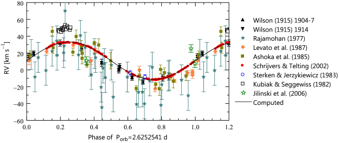
Figure 2: Archival RVs of $\nu$ Cen plotted as a function of orbital phase. The phases were computed from ephemeris (3). The solid line is the RV curve computed from the spectroscopic elements listed in Table 6.

4.2 The RV curve and the spectroscopic orbit

The RVs of $\nu$ Cen are plotted in Fig. 2. For the Schrijvers & Telting (2002) points, the error bars (not shown) would be of about the same size as the symbols plotted in the figure because we assumed the standard error to be equal to 0.6 km s^-1, the standard deviation of the least-squares fit of the sine-curve to these points (see Section 4.1). In addition to the data referenced in Table 4 (filled symbols), the RV measurements of Sterken & Jerzykiewicz (1983), Kubiak & Seggewiss (1982) and Jilinski et al. (2006), i.e. sets (5), (6) and (10) detailed in Table 2, are shown (open symbols). In the case of Sterken & Jerzykiewicz (1983), we plotted only the first and the last of their 49 data-points with the standard errors provided by them. In the case of Jilinski et al. (2006), we converted the MJD of the exposure beginning (which they call HJD in their table 1) to HJD of the middle of the exposure by adding 2400000.5 d, the heliocentric correction and half of the exposure time. In addition, we estimated the standard error from the range of the RVs on HJD 2452413 (the two asterisks at phase $\sim$0.99 in Fig. 2) to be 4.5 km s^-1. As can be seen from the figure, most measurements scatter around those of Schrijvers & Telting (2002); the two exceptions are the measurements of Rajamohan (1977) and Kubiak & Seggewiss (1982). The former show a systematic shift toward smaller RVs, the latter, toward greater RVs. Omitting the Rajamohan (1977) and Kubiak & Seggewiss (1982) data, we computed a spectroscopic orbit by means of the non-linear least squares method of Schlesinger (1910) with weights inversely proportional to the squares of the standard errors of the velocities. The parameters of the orbit are determined by RVs of Schrijvers & Telting (2002) but their standard deviations, by the remaining data. The eccentricity of the orbit turned out to be an insignificant $e=0.009\,\pm\,0.007$. We conclude that the orbit is circular, confirming the result of Wilson (1915). The elements of the orbit are listed in Table 6 and the RV curve computed from these elements is shown in Fig. 2 with the solid line.

Table 6: Orbital elements of $\nu$ Cen.

Orbital period, $P_{\rm orb}$	2.6252541 d (assumed)
Epoch of crossing the gamma axis
from approach to recession, HJDγ	2450893.6658 $\pm$ 0.0031
Eccentricity, $e$	0 (assumed)
$\gamma$ velocity	10.77 $\pm$ 0.09 km s-1
Semi-amplitude of primary’s RVs, $K_{1}$	22.30 $\pm$ 0.12 km s-1
Projected semi-major axis, $a_{1}\sin i$	1.157 $\pm$ 0.006 R☉
Mass function, $f(M)$	0.00302 $\pm$ 0.00005 M☉

4.3 The orbital light-curves and the W-D modelling

The light-curves of $\nu$ Cen are presented in Fig. 3. The data shown are normal points formed in adjacent intervals of 0.02 orbital phase from the blue and red BRITE magnitudes (the upper and lower panel, respectively). The error bars are not shown because they would barely extend beyond the plotted circles: the standard errors ranged from 0.27 to 0.42 mmag for the blue normal points, and from 0.26 to 0.39 mmag for the red normal points. The lines plotted in the figure are the theoretical light-curves, results of the Wilson-Devinney (W-D) modelling to be discussed presently. A least-squares fit of a sum of the $f_{\rm orb}$ and 2$f_{\rm orb}$ sines to the normal points yields blue amplitudes of 5.47$\,\pm\,$0.22 and 0.11$\,\pm\,$0.22 mmag, and red amplitudes of 8.70$\,\pm\,$0.16 and 0.14$\,\pm\,$0.16 mmag, respectively. The 2$f_{\rm orb}$ amplitudes are consistent with the conclusion of Appendix A.1 that no detectable ellipsoidal light-variation is present. Thus, the orbital light-variation is caused solely by the reflection effect.

Figure 3: The light-curves of $\nu$ Cen. Plotted are normal points formed in the adjacent intervals of 0.02 orbital phase from the blue (upper panel), and red (lower panel) BRITE magnitudes. The phases were computed from ephemeris (3). The lines are the theoretical W-D light-curves.

The light curves were subject to modelling by means of the 2015 version of the W-D code (Wilson & Devinney, 1971; Wilson, 1979). In addition to the light curves, the input data for the code included the orbital elements from Table 6 and the primary component’s fundamental parameters $T_{\rm eff,1}={}$22 370 K and $\log g_{1}={}$3.76 from Appendix B.1. The $T_{\rm eff,1}$ was fixed throughout but the final $\log g_{1}$, used only in deriving the limb darkening coefficients, were taken from the W-D solutions after several iterations. The limb darkening coefficients were from the logarithmic-law tables of Walter V. Van Hamme. For the primary component we assumed [M/H] $=0$ and used 421 and 620.5 nm monochromatic coefficients for the blue and red data, respectively. A radiative-envelope albedo of 1.0 was assumed. In treating the reflection effect, we used the detailed model with six reflections (MREF $=2$, NREF $=6$). For the secondary component, bolometric limb-darkening coefficients and a convective-envelope albedo of 0.5 were adopted.

The mass function, $f(M)$, depends on the primary’s mass, $M_{1}$, the secondary’s mass, $M_{2}$, and the inclination, $i$, or — alternatively — on $M_{1}$, $i$, and the mass ratio $q=M_{2}/M_{1}$. Once two of these parameters are fixed, the third can be calculated from $f(M)$ given in Table 6. The evolutionary mass $M_{1}=8.7\,\pm\,$0.3 M_☉ derived for the primary component of $\nu$ Cen in Appendix B.1 is model dependent. Therefore, in order to be certain that the range of $M_{1}$ adopted in the W-D modelling comprises the true primary mass, we assumed a range five times wider than the formal uncertainty of $M_{1}$, i.e. 7.2 to 10.2 M_☉. In a preliminary run we found that the range of $i$ should be limited to $30\degr\leq i<75\degr$ because for $i\geq 75\degr$ the W-D light-curves showed an eclipse not seen in the observed light-curves, while for $i<30\degr$ an ellipsoidal effect, also not present in the observed light-curves, showed up in the W-D light curves. In the $i<30\degr$ models, the distortion of the primary causing the ellipsoidal effect was a consequence of a higher $M_{2}$ and a tighter orbit. In addition, a higher $M_{2}$ and hence greater brightness would be also inconsistent with the lack of the secondary’s lines in the spectrum. The final W-D modelling was therefore done assuming a grid of ($M_{1}$, $i$) $\in$ (7.2 – 10.2 M_☉, 35$\degr$ – 75$\degr$). As it turned out, the $q$ calculated for the whole grid was confined to a rather narrow range of 0.074 – 0.169.

In the ($M_{1}$, $i$) grid, we fitted the W-D light-curves to the normal points shown in Fig. 3 assuming equal weights. The overall standard deviation of the fits were very nearly the same over the whole grid. This is a consequence of the fact that there are three free parameters in the models, the secondary’s effective temperature, $T_{\rm eff,2}$, and the components’ radii, $R_{1}$ and $R_{2}$ (formally, the surface potentials), that can be adjusted to get a satisfactory fit. Thus, the fits do not discriminate between different ($M_{1}$, $i$). The solid lines plotted in Fig. 3 are the W-D light-curves computed with $M_{1}={}$8.695 M_☉ and $i=35\degr$. At the resolution of the figure, the light-curves computed with other ($M_{1}$, $i$) values would be impossible to distinguish from those shown. The ranges of the parameters of the components obtained from the W-D modelling are given in Table 7; they are an order of magnitude greater than the formal standard deviations of the W-D solutions. It is interesting that the primary’s W-D surface gravity is much better constrained than that derived in Appendix B.1 from the photometric indices. In Fig. 4, the components of $\nu$ Cen are plotted using the effective temperature and luminosity of the primary from Appendix B.1, and those of the secondary from Table 7; the ranges of $\log T_{\rm eff,2}$ and $\log(L_{2}/\mbox{L}_{\sun})$ listed in the table define the full lengths of the error bars and the open inverted triangles are placed at their intersection. Also shown in the figure is the ZAMS for the $Z=0.014$ models from Ekström et al. (2012). Given coevality of the components, the position of the secondary relative to the ZAMS indicates its pre-MS status. The secondary’s evolutionary status will be further discussed in Section 6.

Table 7: The ranges of parameters of the components of $\nu$ Cen and $\gamma$ Lup A obtained from the W-D modelling for the given ranges of the mass of the primary.

Parameter	$\nu$ Cen	$\gamma$ Lup A
$M_{1}$ [M☉] (assumed)	$\langle$7.2 – 10.2$\rangle$	$\langle$6.0 – 10.0$\rangle$
$M_{2}$ [M☉]	$\langle$0.59, 1.45$\rangle$	$\langle$0.72, 1.93$\rangle$
$R_{1}$ [R☉]	$\langle$3.93, 4.56$\rangle$	$\langle$3.92, 5.39$\rangle$
$R_{2}$ [R☉]	$\langle$1.30, 2.10$\rangle$	$\langle$2.00, 3.47$\rangle$
$T_{\rm eff,2}$ [K]	$\langle$5790, 6150$\rangle$	$\langle$4140, 7210$\rangle$
$M_{\rm bol,1}$	$\langle$$-$4.43, $-$4.10$\rangle$	$\langle$$-$4.47, $-$3.78$\rangle$
$M_{\rm bol,2}$	$\langle$$+$2.94, $+$4.05$\rangle$	$\langle$$+$2.17, $+$3.78$\rangle$
$\log(L_{1}/\mbox{L}_{\sun})$	$\langle$3.54, 3.67$\rangle$	$\langle$3.41, 3.68$\rangle$
$\log(L_{2}/\mbox{L}_{\sun})$	$\langle$0.28, 0.72$\rangle$	$\langle$0.38, 1.03$\rangle$
$\log(g_{1}/(\mbox{cm\,s}^{-2}))$	$\langle$4.103, 4.132$\rangle$	$\langle$3.867, 4.130$\rangle$
$\log(g_{2}/(\mbox{cm\,s}^{-2}))$	$\langle$3.965, 3.987$\rangle$	$\langle$3.515, 3.803$\rangle$
$L_{3}/(L_{1}+L_{2})_{\rm blue}$	0.0 (assumed)	$\langle$0.31, 1.46$\rangle$
$L_{3}/(L_{1}+L_{2})_{\rm red}$	0.0 (assumed)	$\langle$0.34, 2.18$\rangle$
$q=M_{2}/M_{1}$	$\langle$0.074, 0.169$\rangle$	$\langle$0.099, 0.234$\rangle$
$a$ [R☉]	$\langle$16.0, 18.2$\rangle$	$\langle$16.0, 19.3$\rangle$

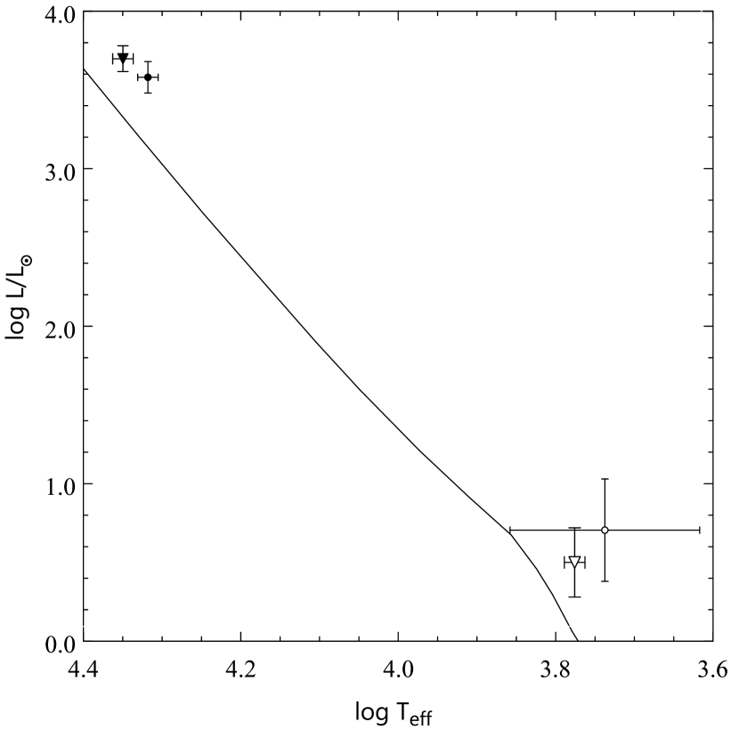
Figure 4: The components of $\nu$ Cen and $\gamma$ Lup A (inverted triangles and circles, respectively) in the HR diagram. The line is the ZAMS from Ekström et al. (2012) for the $Z=0.014$ models with no rotation. For $\log(L_{1}/\mbox{L}_{\sun})<1.0$, the ZAMS for models with rotation is virtually identical with the one shown.

5 The triple system of $\mn@boldsymbol{\gamma}$ Lup

5.1 The SB1 RV curve

All sets of the RV observations of $\gamma$ Lup detailed in Section 3.2 and Table 2 can be phased with the photometric orbital frequency of 0.35090 d^-1 provided that one day is added to all JD epochs of observations of van Hoof et al. (1963) (their UT dates are correct) and a misprint in one epoch of observation of van Albada & Sher (1969) is corrected: in their table 3, April 25.019 should be replaced with April 25.919. In four sets, (11), (14), (15), and (17), the RV measurements are distributed in orbital phase sufficiently well to be fit with the sine curve in which $f_{\rm orb}=0.35090$ d^-1. Using a sine curve is justified because the SB1 orbit of $\gamma$ Lup is circular (see Section 5.4). In fitting Eq. (1), we used the method of least squares with weights inversely proportional to the squares of the standard errors of the velocities. For sets (11) and (14), the standard errors were obtained by multiplying the standard error of an equal-weights fit by $\sqrt{\langle n\rangle/n}$, where $n$ is the number of lines measured and $\langle n\rangle$ is the overall mean of $n$. For set (15), the standard errors were computed from the probable errors provided by Levato et al. (1987). For set (17), the standard errors are given in Table 3. The fits yielded the $\gamma$ velocities to be used in Section 5.2, and the epochs of crossing the $\gamma$-axis from the smaller to greater RV (i.e. from approach to recession), HJD_γ, to be used in Section 5.3.

5.2 Component A is the SB

Given the elements of the $\gamma$ Lup AB visual binary orbit, the parallax of the system and the mass ratio of the components, the temporal variation of the RVs of the components A and B can be computed. After Heintz (1990) derived the elements mentioned in Section 2, a number of interferometric determinations of the position angle $\theta$ and angular separation $\rho$ of $\gamma$ Lup B relative to A became available. In order to update the orbital elements, we compiled a list of $\theta$ and $\rho$ from the US Naval Observatory’s Fourth Catalog of Interferometric Measurements of Binary Stars, assigning weights to the measurements depending on the number of observations used in computing $\theta$ and $\rho$, the scatter of the observations and the telescope size. Zero weight was given to the measurements with $\rho$ grossly deviating from the average run; this was never the case for $\theta$. The updated elements were estimated by bootstrapping with 1 000 resamplings. The elements are listed in Table 8 and the corresponding apparent relative orbit is plotted in Fig 5. The value of $a={}0\aas@@fstack{\prime\prime}$970 from the table and the revised Hipparcos parallax, equal to 7.75$\,\pm\,$0.50 mas (van Leeuwen, 2007), yield the semi-major axis of the relative orbit $a=125.2$ AU. Inserting this value and the period of the AB system $P_{\rm AB}=167.3$ yr into Kepler’s third law, we get the mass of the system $M_{\rm A}+M_{\rm B}=70.1$ M_☉, a value much too large for a pair of B2 stars. The lower bound of the orbital period, $P_{\rm AB}=160.1$ yr, yields a value still greater. Using the upper bound of the orbital period allowed by the solution, $P_{\rm AB}=188.8$ yr, and the corresponding $a=1.394\times 10^{10}$ km, we get $M_{\rm A}+M_{\rm B}=22.7$ M_☉, a value still 5.5 M_☉ greater than the overall mass of the system derived in Section B.2.

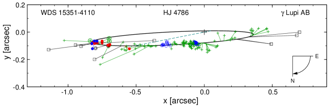
Figure 5: The apparent relative orbit of the $\gamma$ Lup AB (HJ 4786) system. The ellipse corresponds to the solution given in Table 8. The individual measurements are plotted with different symbols, depending on the observing technique. The techniques were the following: micrometric measurements (green pluses; the three discovery measurements made by J. F. W. Herschel in 1835 – 1837 are encircled), visual interferometry (open blue circles), speckle interferometry (filled red circles), CCD, mostly lucky imaging (filled blue circles), Hipparcos and Tycho measurements (black double circles). The data excluded from the fit are plotted as black squares. All measurements are connected with the calculated position in the orbit, corresponding to the epoch of observation. The large plus marks the position of component A and the dashed line is the line of apsides.

Taking the above-mentioned three values of $P_{\rm AB}$ and the corresponding $T$, $e$, $i$ and $\omega$ from Table 8, and assuming $\gamma={}$0.00 km s^-1, we computed the RV curves shown in Fig. 6. Also plotted are the $\gamma$ velocities from the fits carried out in Section 5.1 decreased by 4.12 km s^-1, so that sets’ (14) $\gamma$ (triangle) coincides with the computed RVs of component A for $P_{\rm AB}=167.3$ yr and $q=1.0$ (blue solid line). It is clear from the figure that (i) the $\gamma$ velocities approximately follow the computed RV variation of component A, justifying this section’s heading, and (ii) the available RV data are insufficient to constrain the elements of the visual binary orbit or the component’s mass ratio.

Table 8: Parameters of the visual binary orbit of $\gamma$ Lup AB (HJ 4786).

Parameter	Value
Orbital period, $P_{\rm AB}$ [yr]	167.3${}^{+21.5}_{-7.2}$
Time of periastron passage, $T$ [yr]	1885.7${}^{+2.9}_{-4.0}$
Semi-major axis, $a$ [arcsec]	0.970${}^{+0.343}_{-0.240}$
Eccentricity, $e$	0.826${}^{+0.082}_{-0.181}$
Inclination, $i$ [$\degr$]	93.04${}^{+1.45}_{-0.89}$
Longitude of periastron, $\omega$ [$\degr$]	286.90${}^{+12.0}_{-5.9}$
Position angle of the line of nodes, $\Omega$ [$\degr$]	91.20${}^{+0.52}_{-0.35}$

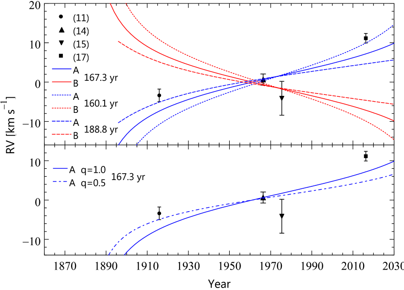
Figure 6: The RVs of the components A and B of $\gamma$ Lup, computed from the orbital elements of Table 8 and the revised Hipparcos parallax, for the B to A mass ratio $q=1.0$ (upper panel), and the RV of component A for $q=1.0$ and 0.5 (lower panel) compared with the $\gamma$ velocities determined in Section 5.1 from the four RV sets detailed in the text (symbols with error bars).

5.3 The light-time effect

Because of the orbital motion around the centre of mass of the AB system, the epochs of observations of $\gamma$ Lup A include a term arising from the light-time effect (LiTE). In particular, the epochs of crossing the $\gamma$-axis from the smaller to greater RV, HJD_γ, derived in Section 5.1, and the epochs of maximum light, HJD_max, to be derived shortly, will be affected. HJD_γ are listed in the second column of Table 9 while HJD_max, in the first column of Table 10. The latter were computed from the least-squares fits of Eq. (2) with $f_{\rm orb}=0.35090$ d^-1 to the Hipparcos, SMEI, and BRITE data. The SMEI data were divided into five adjacent segments of approximately equal duration. Before fitting, the 2014 BRITE magnitudes were pre-whitened with the 1.5389 d^-1 term, and the 2015 blue magnitudes were pre-whitened with the 1.6913 d^-1 term derived in Appendix A.3.

Table 9: The epoch of crossing the $\gamma$-axis from the smaller to greater RV, HJD_γ, the number of cycles, $E$, and the residuals (O – C)_1.0 and (O – C)_0.5 from the $P_{\rm AB}=188.8$ yr, $q=1.0$ and 0.5 ephemerides (see Section 5.3).

Set	HJD${}_{\gamma}-$2400000	$E$	(O – C)1.0	(O – C)0.5
(11)	20811.868 $\pm$ 0.039	$-$12868	$-$0.117	$-$0.015
(14)	39255.415 $\pm$ 0.026	$-$6396	$-$0.269	$-$0.204
(15)	42566.952 $\pm$ 0.116	$-$5234	$-$0.163	$-$0.104
(17)	57482.791 $\pm$ 0.023	0	$-$0.009	$+$0.020

In Fig. 7 there are shown the LiTE O – C curves computed for $\gamma$ Lup A from equation (3) of Irwin (1952) with the 167.3, 160.1 and 188.8-yr elements of Table 8 (the solid, short-dashed and dashed lines, respectively) for two values of the B to A mass ratio, $q=1.0$ (upper panel) and 0.5 (lower panel). Assuming that at a given epoch the orbital phase of HJD_γ is equal to that of HJD_max, i.e. that the maximum light of the SB light-curve occurs when the secondary is at superior conjunction, one can fit the LiTE O – C curves to the HJD_γ and HJD_max from Tables 9 and 10. In the ephemerides $T_{0}+P_{0}E$ obtained in this way, the period $P_{0}$ is equal to the $\gamma$ Lup SB A orbital period, $P_{\rm orb}$, for the epoch of $d({\rm O}-{\rm C})/dE=0$. For the 188.8-yr elements, which yield the smallest value of $M_{\rm A}+M_{\rm B}$ we consider (see Section 5.2), the residuals computed with $q=1.0$ and 0.5, (O – C)_1.0 and (O – C)_0.5, are listed in Tables 9 and 10 and plotted in Fig. 7. The $q=1.0$ residuals fit the computed O – C curve with a slightly smaller standard deviation (0.0071 d) than the $q=0.5$ residuals (0.0076 d).

Table 10: The epoch of maximum light, HJD_max, the number of cycles, $E$, and the residuals (O – C)_1.0 and (O – C)_0.5 from the $P_{\rm AB}=188.8$ yr, $q=1.0$ and 0.5 ephemerides (see Section 5.3).

HJDmax	$E$	(O – C)1.0	(O – C)0.5	Source of
$[{\rm HJD}-2400000]$		[d]	[d]	data
48500.2220(306)	$-$3152	$-$0.1093	$-$0.0626	Hipparcos
52999.9459(125)	$-$1573	$-$0.1690	$-$0.1314	SMEI
53649.7780(156)	$-$1345	$-$0.0840	$-$0.0477	SMEI
54199.7201(142)	$-$1152	$-$0.1472	$-$0.1119	SMEI
54749.7261(133)	$-$959	$-$0.1464	$-$0.1122	SMEI
55351.0101(180)	$-$748	$-$0.1634	$-$0.1305	SMEI
56815.8423(083)	$-$234	$-$0.1118	$-$0.0818	BRITE blue
56815.8671(057)	$-$234	$-$0.0877	$-$0.0576	BRITE red
57180.6374(047)	$-$106	$-$0.0886	$-$0.0593	BRITE blue
57180.6457(051)	$-$106	$-$0.0774	$-$0.0481	BRITE red

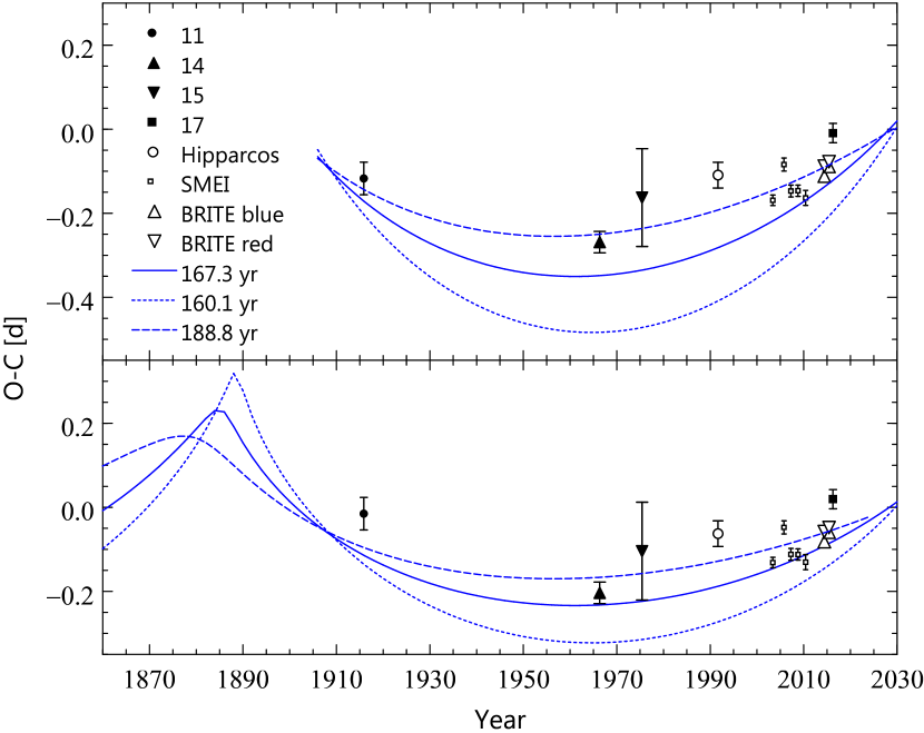
Figure 7: The LiTE O – C curves for $\gamma$ Lup A, computed from the orbital elements of Table 8 (lines) for the B to A mass ratio $q=1.0$ (upper panel) and 0.5 (lower panel), compared with the (O – C)_1.0 and (O – C)_0.5 residuals from Tables 9 and 10 (symbols with error bars).

5.4 The SB RV and the mean light-curves of $\mn@boldsymbol{\gamma}$ Lup A

Using the $P_{\rm AB}=188.8$ yr, $q=1.0$ LiTE O – C curve (dashed line in the upper panel of Fig. 7), we corrected the epochs of the RV and the BRITE observations of $\gamma$ Lup for the LiTE, i.e. reduced the epochs to the centre of mass of the AB system. In addition, we reduced all RV measurements using component’s A computed RVs (blue dashed line in the upper panel of Fig. 6) and removed a systematic difference of 6.4 km s^-1 between sets (14) and (17). Then, we re-determined HJD_γ and HJD_max. The ephemeris obtained from these data

$${\rm HJD}_{\gamma}={\rm HJD}\,2457482.7996(39)+2.8497690(47)\times E.$$ (4)

will be unaffected by the orbital motion of component A provided that the true $P_{\rm AB}$ and $q$ are equal to those we assumed. The initial epoch and the period in ephemeris (4) are close to those of the $P_{\rm AB}=188.8$ yr, $q=1.0$ ephemeris derived in Section 5.3. This comes about because $d{\rm RV}/dt=0$ at the epoch of $d({\rm O}-{\rm C})/d{\rm E}=0$.

The reduced RVs are plotted in Fig. 8 as a function of phase computed using the LiTE-corrected epochs of observations and $P_{\rm orb}$ from ephemeris (4). These data were then used in computing a spectroscopic orbit by means of the non-linear least squares method of Schlesinger (1910) with weights inversely proportional to the squares of the standard errors. The standard errors of sets (11), (14), (15), and (17) were the same as in Section 5.1 while those of set (16) were taken from Table 3. For set (12), we obtained the standard errors from the probable errors Buscombe & Morris (1960) provide, while for set (13) we estimated the standard error from the scatter in the phase diagram. The eccentricity of the orbit turned out to be equal to an insignificant $e=0.044\,\pm\,$0.045. It is thus feasible to assume that the orbit is circular. The elements of a circular orbit are listed in Table 11 and the RV curve computed from these elements is shown in Fig. 8 with the solid line.

An anonymous referee has suggested that the orbital period of the AB binary could be obtained from an assumed value of the mass of the system equal to a sum of masses of two B2 stars. We carried out this exercise using the mass of the system of 17.2$\,\pm\,$0.7 M_☉ derived in Section B.2 and the same data as in the first paragraph of Section 5.2. We obtained $P_{\rm AB}={}$198.3$\,\pm\,$5.4 yr and the remaining orbital elements rather close to those of Heintz (1990) mentioned in Section 2. If plotted in the upper panel of Fig. 6, the RVs computed with the $P_{\rm AB}={}$198.3-yr elements would very nearly coincide with those computed with the $P_{\rm AB}={}$188.8-yr elements. A similar result is obtained for the $O-C$ shown in Fig. 7. In addition, the elements of the $\gamma$ Lup A spectroscopic orbit obtained from the HJD and RV corrected for LiTE with the $P_{\rm AB}={}$198.3-yr elements differ from those in Table 11 by much less than 1$\sigma$: $K_{1}$, $a_{1}\sin i$ and $f(M)$ differ by 0.5$\,\pm\,$1.4 km s^-1, 0.03$\,\pm\,$0.08 R_☉ and 0.0003$\,\pm\,$0.0008 M_☉, respectively. Clearly, there exists an interval of mass of $\gamma$ LupAB such that for a mass from this interval there is a value of $P_{\rm AB}$ which accounts for the observed temporal variation of RV and $O-C$. We believe that more measurements of $\theta$ and $\rho$ of the system are needed to narrow down this interval. Whether the model-independent mass of the system derived from the observed orbit will then agree with the model-dependent mass obtained in Section B.2 remains to be seen.

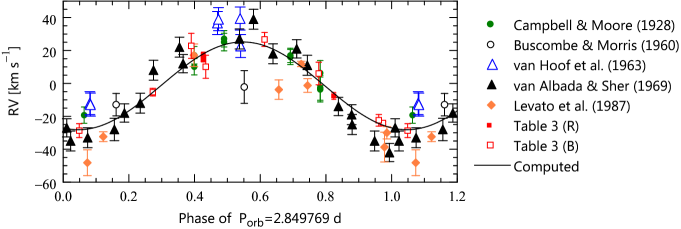
Figure 8: The RVs of $\gamma$ Lup, corrected for the LiTE as explained in the text, plotted as a function of the orbital phase. The epoch of phase zero is HJD 2457482. The solid line is the RV curve computed from the spectroscopic elements listed in Table 11.

Table 11: Orbital elements of $\gamma$ Lup A computed under assumption of zero eccentricity from the LiTE-corrected RV shown in Fig. 8. HJD_γ is the epoch of crossing the $\gamma$-axis from the smaller to greater RVs (i.e. from approach to recession).

Orbital period, $P_{\rm orb}$	2.849769 d (assumed)
Epoch of crossing $\gamma$ axis, HJDγ	2457482.846 $\pm$ 0.021 d
Eccentricity, $e$	0 (assumed)
$\gamma$ velocity	$-$1.5 $\pm$ 0.7 km s-1
Semi-amplitude of primary’s orbit, $K_{1}$	26.7 $\pm$ 1.0 km s-1
Projected semi-major axis, $a_{1}\sin i$	1.50 $\pm$ 0.05 R☉
Mass function, $f(M)$	0.0056 $\pm$ 0.0006 M☉

Let us now turn to the question whether correcting the epochs of observations for the LiTE would affect results of frequency analysis of the BRITE data. As can be seen from Fig. 7, the LiTE corrections to the epochs of observations over the time interval covered by the BRITE data can be expressed by a linear function of time, $a+bt$, where $a$ and $b$ are constants. In other words, the LiTE-corrected epochs of observations are shifted by $a$ and scaled by $1+b$. From the well-known properties of the Fourier transform it follows that the time shift translates in the frequency domain into a phase shift, while the scaling, into scaling the frequencies and amplitudes by the reciprocal of $1+b$. Since $b\approx 1.5\times 10^{-5}$, the answer to our question is no. More precisely, the LiTE corrections would have negligible effect on the frequencies and amplitudes derived in Appendices A.2 and A.3.

Using the 2014 and 2015 blue and red magnitudes (see Appendix A.3) with the LiTE-corrected epochs of observations and $P_{\rm orb}$ from ephemeris (4), we plot the blue and red phase diagrams in Fig. 9. The data plotted in the figure are normal points, computed in the adjacent intervals of 0.01 orbital phase. The standard errors, ranging from 0.25 to 0.35 mmag for the blue normal points and from 0.24 to 0.36 mmag for the red normal points, are not shown. The solid lines are the theoretical light-curves, results of the W-D modelling detailed in Section 5.5. A least-squares fit of a sum of the $f_{\rm orb}$ and 2$f_{\rm orb}$ sines to the normal points yields the blue amplitudes of 5.92$\,\pm\,$0.10 and 0.14$\,\pm\,$0.10 mmag, and the red amplitudes of 8.54$\,\pm\,$0.12 and 0.44$\,\pm\,$0.12 mmag. In the latter case, the phase difference between the $f_{\rm orb}$ and 2$f_{\rm orb}$ sines is equal to 0.21$\,\pm\,$0.14 rad, excluding ellipsoidal effect as the cause of the 2$f_{\rm orb}$ term. We conclude that the orbital light-variation is caused solely by the reflection effect. The amplitudes and the phase difference agree with the results presented in Section A.3.

Figure 9: The orbital light-curves of $\gamma$ Lup. Plotted are normal points formed in the adjacent intervals of 0.01 orbital phase from the combined 2014 and 2015 blue (upper panel) and red (lower panel) BRITE magnitudes. The epoch of phase zero is HJD 2457482. The lines are the theoretical W-D light-curves computed with $M_{1}={}$8.093 M_☉ and $i=55\degr$.

5.5 The W-D modelling

In the W-D modelling of the light curves of $\gamma$ Lup we used the orbital elements from Table 11 and the fundamental parameters $T_{\rm eff,1}={}$20 790 K and $\log g_{1}={}$3.94 from Appendix B.2. As in the case of $\nu$ Cen, the $T_{\rm eff,1}$ was fixed throughout but the final $\log g_{1}$ were taken from the W-D solutions after several iterations. The remaining details of the W-D modelling were also the same as in the case of $\nu$ Cen (see Section 4.3), except that a third light was included in order to account for component B. The third light’s brightness was kept as a free parameter because fixing it at a level consistent with the Hp magnitudes of the components (see Section 2) resulted in a divergent solution. As in the case of $\nu$ Cen, the range of $M_{1}$ was assumed to span five times the uncertainty obtained in Appendix B.2. The results of the W-D modelling, listed in Table 7, bear many similarities to the results for $\nu$ Cen (Section 4.3): (i) the mass ratio is low, $q=0.15^{+0.09}_{-0.05}$, (ii) the W-D light-curves fit the normal points with very nearly the same overall standard deviation over the whole ($M_{1}$, $i$) grid, (iii) the position of the secondary relative to the ZAMS indicates its pre-MS status (see Fig. 4). The secondary’s evolutionary status will be further discussed in Section 6.

6 Discussion and conclusions

Using stellar parameters and the results of the W-D modelling of the reflection effect in $\nu$ Cen and $\gamma$ Lup A, we concluded in Sections 4.3 and 5.5 that the secondaries in both systems are in the pre-MS stage of evolution. Thus, as we already mentioned in Section 1, the systems can be regarded as non-eclipsing counterparts of the NEBs, to be referred to in the following as NnonEBs. In order to strengthen this conclusion, we compare in Fig. 10 the radii, the age, and the range of reflection effect of $\nu$ Cen and $\gamma$ Lup A with those of the LMC NEBs using the parameters of $\nu$ Cen and $\gamma$ Lup A from Table 7 (the ranges of the parameters are plotted as error bars) and those of the LMC NEBs from tables 1 and 2 of Moe & Di Stefano (2015). First of all, the radii of the secondaries are significantly larger than the zero-age main sequence (ZAMS) values for stars with the same masses (upper left-hand panel of the figure). A more convincing argument that $\nu$ Cen and $\gamma$ Lup A are indeed NnonEBs comes from the positions of their secondaries in the mass-age diagram (upper right-hand panel). The ages of the systems in the diagram were taken from Appendices B.1 and B.2, where they are determined from the position of the primary components in the HR diagram in relation to the evolutionary tracks. As in the case of the LMC NEBs, both secondaries are located on the pre-MS side of the line which divides the pre-MS and MS regions. The two lower panels of Fig. 10 show parameters characterising the light curves. The NnonEBs $\nu$ Cen and $\gamma$ Lup A can be plotted only in the left-hand panel, in which they occupy a short-$P_{\rm orb}$ extension of the area occupied by the LMC NEBs. Also shown in Fig. 10 are two SB1 eclipsing binaries 16 (EN) Lac and $\mu$ Eri mentioned in Section 1. 16 (EN) Lac is plotted with the parameters from Jerzykiewicz et al. (2015), while $\mu$ Eri, with the parameters computed using the data from tables 3 and 4 and fig. 11 of Jerzykiewicz et al. (2013). Because of the ratio of the radii $k=R_{2}/R_{1}$ of only $\approx 0.25$ and a relatively long orbital period of 12.1 d, the range of the reflection effect in 16 (EN) Lac is smaller than 5 mmag. The pre-MS status of the star’s secondary component is based on the analysis of the ground-based eclipse light-curve (Pigulski & Jerzykiewicz, 1988; Jerzykiewicz et al., 2015) and an unpublished eclipse light-curve obtained by one of the authors (MJ) from the NASA Transiting Exoplanet Survey Satellite (TESS, Ricker et al., 2015) observations. In the case of $\mu$ Eri, the orbital period is about 1.6 times shorter than that of 16 (EN) Lac but the reflection effect is below the detection threshold because of the small $k\approx 0.135$. Still, as can be seen from Fig. 10, the pre-MS status of the secondary is evident. We conclude that 16 (EN) Lac and $\mu$ Eri should be regarded as bona fide NEBs. Note that since it was the reflection signature in the eclipsing light-curves which Moe & Di Stefano (2015) used to single out the NEBs from the OGLE data, objects similar to 16 (EN) Lac and $\mu$ Eri would have passed undetected in their search.

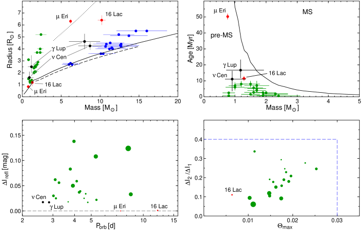
Figure 10: The stars discussed in the present paper in relation to the LMC NEBs. Upper left: The mass-radius diagram for the primaries (blue) and the secondaries (green) of the LMC NEBs. The components of $\nu$ Cen and $\gamma$ Lup A are plotted as black dots, those of 16 (EN) Lac and $\mu$ Eri, as red dots. The solid line is the ZAMS mass-radius relation for the $Z=0.014$ models with no rotation from Ekström et al. (2012) for $M\geq 0.8$ M_⊙, and from Tognelli, Prada Moroni & Degl’Innocenti (2011) for $M<0.8$ M_⊙. The dashed line is the ZAMS relation for the non-rotating $Z=0.006$ models (i.e., those with the average metallicity of the LMC) from Georgy et al. (2013). Finally, the dotted line is the terminal-age main sequence (TAMS) relation for the above-mentioned Ekström et al. (2012) models. Upper right: The mass-age relation for the secondaries of the LMC NEBs, $\nu$ Cen, $\gamma$ Lup A, 16 (EN) Lac, and $\mu$ Eri. The line defines the border between the pre-MS and MS regions. The values of the pre-MS phase duration were derived from the models of Tognelli et al. (2011). Lower left: The range of the reflection effect in the $I$ band, $\Delta I_{\rm refl}$, versus orbital period, $P_{\rm orb}$ for the LMC NEBs (green), $\nu$ Cen and $\gamma$ Lup A (black), and 16 (EN) Lac (red). The diameters of the symbols are proportional to the stellar radii. Lower right: The ratio of the eclipse depth versus the width of the wider eclipse, $\Theta_{\rm max}$, for the LMC NEBs and 16 (EN) Lac. For the latter, these parameters were derived from an eclipse light-curve obtained from the NASA Transiting Exoplanet Survey Satellite (TESS, Ricker et al., 2015) observations. The dashed lines contain the LMC NEBs region shown in the central panel of fig. 1 of Moe & Di Stefano (2015).

As far as we are aware, $\nu$ Cen and $\gamma$ Lup A are the only known NnonEBs, i.e early B-type non-eclipsing SB systems such that (i) their observed orbital light-variation is caused solely by the reflection effect, and (ii) the secondary component is in a pre-MS evolutionary phase. In order to verify this and prepare the ground for a future photometric program, we have searched the literature for the light-variability information about all 169 B0 – B5 non-eclipsing SB systems listed in The Ninth Catalogue of Spectroscopic Binary Orbits (Pourbaix et al., 2004). Apart from $\nu$ Cen and $\gamma$ Lup A, we found only 17 systems with the orbital period equal to the light-variation period, all with primaries of spectral type B3 or earlier. In three cases the secondary component is known to be a compact object, a neutron star or a white dwarf, while in 13, the light curve is a double wave implying an ellipsoidal variation. Only one system, CX Dra, with an orbital period equal to 6.696 d, exhibits a sinusoidal light-variation of this period, albeit with a large amount of scatter, and the phase relation between the RV and light variation characteristic of the reflection effect (Koubský et al., 1980). The scatter is mainly due to the fact that CX Dra is an interacting Be binary showing variations on time-scales from days to years. Koubský et al. (1980) suggest that a combination of ellipsoidal and reflection effects is responsible for the orbital light-variation. However, using the well-known formula for the amplitude, $\delta m$, of the ellipsoidal light-variation (see e.g. Ruciński, 1970) and the spectroscopic orbital parameters of the system (Koubský, 1978) we find $\delta m\loa 0.3$ mmag. Thus, CX Dra meets condition (i). G. D. Penrod (1985, private communication to Horn et al. 1992) detected the lines of the secondary component and estimated the MK type to be F5 III. The orbit of the secondary component was derived by Horn et al. (1992). These authors concluded that the component is a mid-F luminosity III star filling its Roche lobe. This conclusion is at variance with the result of Guinan, Koch & Plavec (1984), obtained by means of a thorough W-D modeling, that the system is detached. In any case, CX Dra does not meet condition (ii). We conclude that no other NnonEBs than $\nu$ Cen and $\gamma$ Lup A are known. However, there is a number of B0 – B5 non-eclipsing SB systems which in the Hipparcos Epoch Photometry have Hp ranges from two to several mmags but were not classified as periodic variables. Re-observed with satellite photometers, some of these systems may turn out to be NnonEBs.

As discussed in some detail by Moe & Di Stefano (2015), the study of nascent binaries may be of great importance for our understanding of the formation of low-mass-ratio binaries and the origin of such objects as type Ia supernovae, low-mass X-ray binaries and millisecond pulsars. The discussion would benefit from including Galactic counterparts of the LMC nascent binaries, eclipsing or otherwise. They should be searched for among young binaries. We have already found several candidates in young open clusters and associations but a detailed discussion of these objects is beyond the scope of this paper.

Data Availability

The raw BRITE data are available from BRITE Public Data Archive (https://brite.camk.edu.pl/pub/index.html). The raw SMEI data are available via the link given in Section 3.1. The processed (decorrelated) BRITE and SMEI data are available from the first author upon request. The other data are available from their respective public databases.

Appendix A Frequency analysis

A.1 $\mn@boldsymbol{\nu}$ Cen

For the purpose of frequency analysis, the reduced BAb and BLb magnitudes of $\nu$ Cen (Table 1) were combined into one data set of blue-filter magnitudes, and the reduced BTr and UBr magnitudes, into one data set of red-filter magnitudes. We shall refer to the two data sets as the red and blue data, respectively. The periodograms using these data were computed in the frequency range from 0 to 20 d^-1. The highest peaks in the periodograms of both data sets occurred at the orbital frequency (Section 4.1). The periodograms of the blue data, the red data and the blue and red data combined, pre-whitened with the orbital frequency, are shown in Fig. 11. Also shown in the figure are the mean noise levels, $N$, and 4$N$, the popular detection threshold set by Breger et al. (1993). As can be seen from the figure, there are no peaks in the periodograms exceeding 0.7 mmag. In particular, the blue and red amplitude at 2$f_{\rm orb}$ is equal to 0.1 mmag, so that an ellipsoidal light-variation, if any, would have the amplitude less than or equal to 0.1 mmag in both colours. At the frequencies corresponding to the putative $\beta$ Cephei-type periods of 0.1750, 0.1690156 and 0.1696401 d, found by Rajamohan (1977), Kubiak & Seggewiss (1982) and Ashoka et al. (1985), the blue and red amplitudes do not exceed 0.2 mmag. One peak in the top panel of Fig. 11 has $S/N$ slightly greater than 4, and a few ones in the middle panel have $S/N$ slightly smaller than 4, but none has a counterpart in the other panel. We conclude that in the data pre-whitened with the orbital frequency there are no periodic terms with an amplitude exceeding 0.7 mmag. In the periodogram of the pre-whitened blue and red data combined (bottom panel), there are no peaks exceeding 0.5 mmag. We thus confirm the results of Shobbrook (1978), Percy et al. (1981) and Sterken & Jerzykiewicz (1983) who found no short-period brightness variation, and strengthen that of Cuypers et al. (1989) who found no variation, other than the orbital one, with an amplitude exceeding 2 mmag (Section 2).

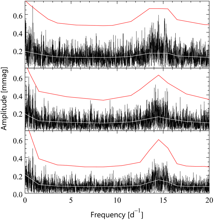
Figure 11: The periodograms of the blue (top), red (middle) and blue and red combined (bottom) BRITE magnitudes of $\nu$ Cen pre-whitened with the orbital frequency. The mean noise levels and four times those are indicated (the white and red lines, respectively).

A.2 $\mn@boldsymbol{\gamma}$ Lup: the 2014 and 2015 data analyzed separately

After combining the reduced 2014 BAb and BLb magnitudes of $\gamma$ Lup into one set of blue magnitudes, and the reduced 2014 UBr and BTr magnitudes, into one set of red magnitudes, we computed periodograms in the same way as we did previously for $\nu$ Cen (Section A.1). In both periodograms, the frequency of the highest peak was equal to the orbital frequency of 0.35090 d^-1 to within 0.015 of the frequency resolution of the data. The periodograms of the blue and red magnitudes pre-whitened with the orbital frequency are shown in the upper and lower panels of Fig. 12, respectively. In both panels, the highest peak occurs at 1.5389 d^-1. At this frequency, the amplitude is equal to 0.7 mmag and the signal-to-noise ratio $S/N>4$ in the upper panel, and the amplitude is equal to 0.6 mmag and $S/N\approx 4$ in the lower panel. The blue to red amplitude ratio and the blue minus red phase difference of the 1.5389 d^-1 sinusoid amount to 1.13$\,\pm\,$0.16 and 0.43$\,\pm\,$0.14 rad, respectively. These numbers are well within the range of values predicted for high radial-order, low harmonic-degree g-mode pulsations of B-stars models (see e.g. Townsend, 2002).

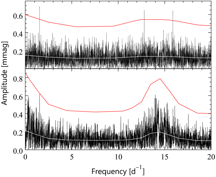
Figure 12: The periodograms of the 2014 blue (upper panel) and red (lower panel) BRITE magnitudes of $\gamma$ Lup pre-whitened with the orbital frequency. The mean noise levels and four times those are indicated (the white and red lines, respectively).

The periodograms of the 2015 blue and red magnitudes pre-whitened with the orbital frequency are shown in the upper and lower panel of Fig. 13, respectively. The highest peak in the upper panel occurs at 1.6913 d^-1, while the highest peak in the lower panel, at 0.3441 d^-1. The former has $S/N>4$, while the latter, $S/N\approx 4$. However, none has a counterpart in the other panel, so that both are probably spurious. The 2014 1.5389 d^-1 term was not present in 2015.

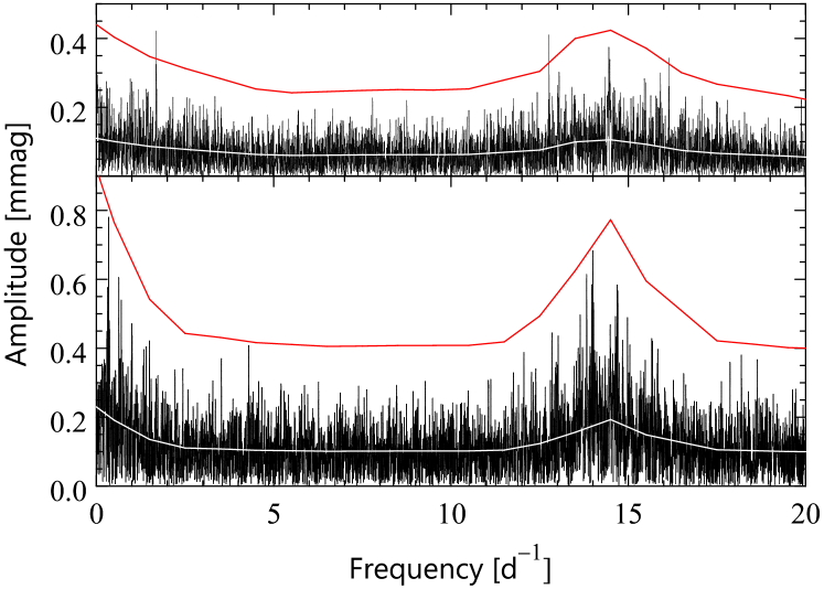
Figure 13: The same as in Fig. 12 but for the 2015 blue (upper panel) and red (lower panel) BRITE magnitudes of $\gamma$ Lup pre-whitened with the orbital frequency.

A.3 $\mn@boldsymbol{\gamma}$ Lup: the 2014 and 2015 data combined

Before combining the 2014 and 2015 blue magnitudes into a single data set, we pre-whitened the 2014 blue magnitudes with the frequency of 1.5389 d^-1, and the 2015 blue magnitudes with the frequency of 1.6913 d^-1. Before combining the 2014 and 2015 red magnitudes, we pre-whitened the 2014 red magnitudes with the frequency of 1.5389 d^-1. This was done because combining the data without pre-whitening resulted in periodograms with peaks close to 1.5389 and 1.6913 d^-1, although not so high as those in the 2014 and 2015 periodograms. The highest peaks in the periodograms of the combined 2014 and 2015 blue and red magnitudes occurred at the same frequency of 0.35088 d^-1, a value very nearly equal to the orbital frequency. The periodograms of the blue data, the red data, and the blue and red data combined, pre-whitened with the orbital frequency, are shown in the top, middle and bottom panel of Fig. 14, respectively. There are no peaks exceeding 4$N$ in the top and middle panels. In the top panel, the highest peak, with $S/N=3.6$, occurs at 0.9554 d^-1. In the middle panel, the two highest peaks, with $S/N=3.9$ and 3.6, occur at 0.3176 and 0.7014 d^-1. The latter frequency is close to 2$f_{\rm orb}$. The amplitude of the sinusoid of this frequency is equal to 0.5 mmag and the phase differs from that of the $f_{\rm orb}$ sinusoid by an insignificant 0.2$\,\pm\,$0.2 rad. Thus, the red orbital light-curve does not deviate within errors from a strictly sinusoidal shape. The same is true for the blue orbital light-curve because the amplitude of 2$f_{\rm orb}$ in the top panel of Fig. 14 amounts to 0.1 mmag. Finally, the periodogram of the blue and red data combined (bottom panel of Fig. 14) shows peaks close to the above-mentioned frequencies 0.3176, 0.7014 and 0.9554 d^-1, and also peaks at 0.3725 and 1.4077 d^-1, all with $S/N\approx 4.0$. It is doubtful that any of these frequencies, except the 0.7014 d^-1 one, represents a variation intrinsic to $\gamma$ Lup. Note that (i) because of the ambiguity mentioned in Section 2, either component A or B would be responsible for any of the frequencies discussed above except $f_{\rm orb}$ and 2$f_{\rm orb}$ (Section 5.2), and (ii) the amplitude of a variation of component A would suffer from light dilution caused by component B, and vice versa.

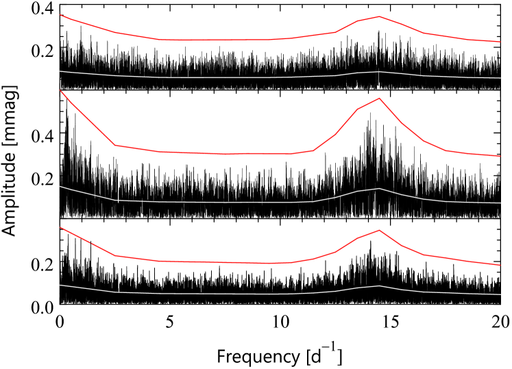
Figure 14: The periodograms of the 2014 and 2015 blue (top), red (middle) and blue and red combined (bottom) BRITE magnitudes of $\gamma$ Lup, modified as explained in the text, pre-whitened with the orbital frequency. The mean noise levels and four times those are indicated (the white and red lines, respectively).

Appendix B Fundamental parameters

B.1 $\mn@boldsymbol{\nu}$ Cen

We shall now derive the fundamental parameters of $\nu$ Cen. From the star’s Strömgren indices $b-y$ and $c_{1}$ given by Hauck & Mermilliod (1998) we obtain $c_{0}=0.082$, $(b-y)_{0}=-0.109$, $E(b-y)=0.007$, and $E(B-V)=0.009$ mag by means of the canonical method of Crawford (1978). From $c_{0}$ we get the effective temperature, $T_{\rm eff}=22\,267$ K, and the bolometric correction, ${\rm BC}=-2.25$ mag, using the calibration of Davis & Shobbrook (1977), $T_{\rm eff}=22\,550$ K using UVBYBETA and 22 289 K using the calibration of Sterken & Jerzykiewicz (1993). The close agreement of these $T_{\rm eff}$ values is due to the fact that the three temperature calibrations rely heavily on the OAO-2 absolute flux calibration of Code et al. (1976). Taking a straight mean of the above three values we arrive at $T_{\rm eff}=22\,370$ K. Realistic standard deviations of the effective temperatures of early-type stars, estimated from the uncertainty of the absolute flux calibration, amount to about 3 % (Napiwotzki et al., 1993; Jerzykiewicz, 1994) or 670 K for the $T_{\rm eff}$ in question. The standard deviation of BC we estimate to be 0.20 mag.

The surface gravity of a B-type star can be obtained from its $\beta$ index. Taking the $\beta$ index of $\nu$ Cen from Hauck & Mermilliod (1998) and $c_{0}$ from the preceding paragraph, we get $\log g=3.76$ by means of UVBYBETA. According to Napiwotzki et al. (1993), the uncertainty of the $\beta$-index surface gravities of hot stars is equal to 0.25 dex; we shall adopt this value as the standard deviation of the star’s $\log g$.

The revised Hipparcos parallax of $\nu$ Cen is equal to 7.47$\,\pm\,$0.17 mas (van Leeuwen, 2007). Taking the star’s $V$ magnitude from Mermilliod (1991), $E(B-V)$ from the first paragraph of this section and assuming $R_{V}=3.2$ we get $M_{V}=-2.25\,\pm\,0.05$ mag. This value and BC yield $M_{\rm bol}=-4.50\,\pm\,0.21$ mag and $\log L/{\rm L}_{\sun}=3.70\,\pm\,0.08$. In computing $\log L/$L_☉, we assumed M${}_{{\rm bol}{\sun}}=4.74$ mag, a value consistent with BC${}_{\sun}=-0.07$ mag, the zero point of the bolometric-correction scale adopted by Davis & Shobbrook (1977). In summary, the fundamental parameters of $\nu$ Cen are: $T_{\rm eff}=22\,370\,\pm\,670$ K, $\log g=3.76\,\pm\,0.25$, $\log L/{\rm L}_{\sun}=3.70\,\pm\,0.08.$ Percentage-wise, $T_{\rm eff}$ is best constrained, while $\log g$, the worst. In the PASTEL catalogue of stellar atmospheric parameters (Soubiran et al., 2016) one finds $T_{\rm eff}=22\,570\,\pm\,1810$ K, a value obtained by Sokolov (1995) from the continuum between 320 and 360 nm. No $\log g$ of $\nu$ Cen is listed in the catalogue.

Since the bolometric magnitude of the secondary component of $\nu$ Cen is at least 7.4 mag fainter than that of the primary (Table 7), so that it is at least 5 mag fainter in $V$ than the primary, the fundamental parameters $T_{\rm eff}$, $\log L/$L_☉ and $\log g$ just derived pertain to the latter; in Section 4.3 we refer to them as $T_{\rm eff,1}$, $\log L_{1}/$L_☉ and $\log g_{1}$. Using the first two parameters, we plot the primary component in Fig. 15. Also shown in the figure are evolutionary tracks computed by means of the Warsaw-New Jersey evolutionary code (see e.g. Pamyatnykh et al., 1998), assuming no convective-core overshooting, the initial abundance of hydrogen $X=0.7$, the metallicity $Z=0.015$, the OPAL equation of state (Rogers & Nayfonov, 2002) and the OP opacities (Seaton, 2005) for the heavy element mixture of Asplund et al. (2009). The tracks were kindly provided by Professor J. Daszyńska-Daszkiewicz. As can be seen from Fig. 15, the primary component of $\nu$ Cen is in the MS stage of evolution. The evolutionary mass and age, estimated from the position of the inverted triangle in the figure relative to the $V_{\rm rot}=80$ km s^-1 evolutionary tracks, are equal to 8.7$\,\pm\,$0.3 M_☉ and 11.1${}^{+5.2}_{-7.6}$ Myr. The most recent value of $V_{\rm rot}\sin i$, measured on high signal-to-noise-ratio spectrograms, is equal to 65$\,\pm\,$6 km s^-1 (Brown & Verschueren, 1997), so that the $V_{\rm rot}$ value we assumed corresponds to the inclination of the rotation axis of 54${}^{+8}_{-6}$ deg. We believe that in view of the large errors of $\log T_{\rm eff,1}$ and $\log L_{1}/$L_☉, the contribution of the uncertainty in $V_{\rm rot}$ to the final error of the evolutionary mass and age is negligible. The evolutionary age we derived is smaller than the MS turnoff age of 17$\,\pm\,$1 Myr obtained for UCL by Mamajek, Meyer & Liebert (2002), but the difference is still within the errors. Our value is close to the age of $\sim$10 Myr obtained from the strength of Li 670.8 nm absorption line by Song, Zuckerman & Bessell (2012).

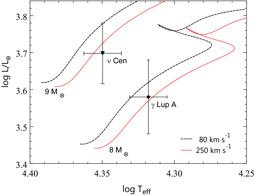
Figure 15: The primary components of $\nu$ Cen and $\gamma$ Lup A (inverted triangle and filled circle with error bars, respectively) in the HR diagram plotted using the effective temperature derived from photometric indices, and the luminosity from the $V$ magnitude, photometric indices and the Hipparcos parallax (see Section B.1 for $\nu$ Cen and B.2 for $\gamma$ Lup A). The lines are the $X=0.7$, $Z=0.015$ evolutionary tracks for 8 and 9 M_☉ and the rotation velocity listed in the bottom right corner.

B.2 $\mn@boldsymbol{\gamma}$ Lup

We shall now derive fundamental parameters of $\gamma$ Lup A assuming that the components A and B, because of their very nearly equal brightness (Section 2), have identical photometric indices, equal to the observed, combined values. From the star’s Strömgren indices $b-y$ and $c_{1}$ (Hauck & Mermilliod, 1998) we get $c_{0}=0.141$, $(b-y)_{0}=-0.103$, $E(b-y)=0.006$ and $E(B-V)=0.008$ mag by means of the canonical method of Crawford (1978). Then, using the same procedures and calibrations as in the case of $\nu$ Cen (Section B.1), we obtain $T_{\rm eff}=20\,790\,\pm\,620$ K, ${\rm BC}=-2.10\,\pm\,0.20$ mag and $\log g=3.94\,\pm\,0.25$. In order to derive component’s A logarithmic luminosity, $\log(L_{\rm A}/{\rm L}_{\sun})$, we first computed the $V$ magnitudes from the Hp magnitudes (Section 2) using the Harmanec (1998) transformation with the $B-V$ and $U-B$ indices from Mermilliod (1991). The result is $V_{\rm A}=3.468$ and $V_{\rm B}=3.582$ mag. The combined $V$ magnitude of $\gamma$ Lup computed from $V_{\rm A}$ and $V_{\rm B}$ is 2.771 mag, in good agreement with $V=2.780\,\pm\,0.013$ mag given by Mermilliod (1991). Moreover, the B minus A $V$-magnitude difference implies an insignificant $B-V$ difference of 0.005 mag, consistent with the assumption made at the beginning of this paragraph. From the revised Hipparcos parallax, equal to $7.75\,\pm\,0.50$ mas (van Leeuwen, 2007), the $E(B-V)$ derived above and $R_{V}=3.2$ we get $M_{V}^{A}=-2.11\,\pm\,0.14$ mag. This value and BC yield $M_{\rm bol}^{A}=-4.21\,\pm\,0.24$ mag. In summary, the fundamental parameters of $\gamma$ Lup A are: $T_{\rm eff}=20\,790\,\pm\,620$ K, $\log g=3.94\,\pm\,0.25$ and $\log(L/{\rm L}_{\sun})=3.58\,\pm\,0.10$. As in the case of $\nu$ Cen, $T_{\rm eff}$ is best constrained, while $\log g$, the worst.

The secondary component of $\gamma$ Lup A is about 4.5 to 5.5 mag fainter than the primary (Table 7). Thus, the fundamental parameters $T_{\rm eff}$, $\log L/$L_☉ and $\log g$ just derived pertain to the latter; in Section 5.5 we refer to them as $T_{\rm eff,1}$, $\log L_{1}/$L_☉ and $\log g_{1}$. Using the first two parameters, we plot the primary component in Fig. 15. As can be seen from the figure, the primary component falls very nearly on the MS branch of the 8 M_☉, $V_{\rm rot}=250$ km s^-1 evolutionary track. Its evolutionary mass and age, estimated from the position of the circle relative to the track, are equal to 8.0 $\pm$ 0.4 M_☉ and $16.7^{+5.0}_{-6.6}$ Myr. According to Głębocki & Gnaciński (2005), $V_{\rm rot}\sin i$ of $\gamma$ Lup is equal to $236\,\pm\,5$ km s^-1, so that the $V_{\rm rot}$ value we assumed is close to a lower limit because it corresponds to the inclination of the rotation axis of $71^{+4}_{-3}$ deg. However, the evolutionary mass and age are rather insensitive to $V_{\rm rot}$ (see below). Unlike the case of $\nu$ Cen, the evolutionary age we derived is very nearly equal to the UCL’s MS turnoff age of $17\,\pm\,1$ Myr (Mamajek et al., 2002). Component B is not plotted in Fig. 15 because it would almost coincide with A. Its evolutionary mass and age would be very nearly equal to those of A, provided it had $V_{\rm rot}=250$ km s^-1. If $V_{\rm rot}=0$ km s^-1, the evolutionary mass and age would become 7.8 $\pm$ 0.4 M_☉ and $17.5^{+5.0}_{-6.6}$ Myr. Since the difference between the evolutionary masses is much smaller than 1$\sigma$, we conclude that the sum of evolutionary masses of the spectroscopic primary of A and that of B is equal to about 15.9 $\pm$ 0.6 M_☉. Assuming the mass of the spectroscopic secondary of A to be equal to 1.3$\,\pm\,$0.3 M_☉, i.e. the middle of the range of $M_{2}$ in Table 7 with an estimated uncertainty, and assuming that B is single, we get 17.2$\,\pm\,$0.7 M_☉ for the overall mass of the AB system, and 0.86$\,\pm\,$0.12 for the B to A mass ratio. The overall mass of the AB system is thus about 5.5 M_☉ smaller than $M_{\rm A}+M_{\rm B}$ derived in Section 5.2 for $P_{\rm AB}=188.8$ yr. Hopefully, this discrepancy will be removed when more measurements of the position angle and angular separation of $\gamma$ Lup B relative to A, and therefore a better visual orbit of $\gamma$ Lup AB than that given in Table 8 become available.

References

- Ashoka & Padmini (1992) Ashoka B. N., Padmini V. N., 1992, Ap&SS, 192, 79
- Ashoka et al. (1985) Ashoka B. N., Surendiranath R., Rao N. K., 1985, Acta Astron., 35, 395
- Asplund et al. (2009) Asplund M., Grevesse N., Sauval A. J., Scott P., 2009, ARA&A, 47, 481
- Baade (1987) Baade D., 1987, Information Bulletin on Variable Stars, 3123
- Breger et al. (1993) Breger M., et al., 1993, A&A, 271, 482
- Brown & Verschueren (1997) Brown A. G. A., Verschueren W., 1997, A&A, 319, 811
- Buscombe & Morris (1960) Buscombe W., Morris P. M., 1960, MNRAS, 121, 263
- Campbell & Moore (1928) Campbell W. W., Moore J. H., 1928, Publications of Lick Observatory, 16, 1
- Code et al. (1976) Code A. D., Bless R. C., Davis J., Brown R. H., 1976, ApJ, 203, 417
- Crawford (1978) Crawford D. L., 1978, AJ, 83, 48
- Cuypers et al. (1989) Cuypers J., Balona L. A., Marang F., 1989, A&AS, 81, 151
- Davis & Shobbrook (1977) Davis J., Shobbrook R. R., 1977, MNRAS, 178, 651
- ESA (1997) ESA ed. 1997, The HIPPARCOS and TYCHO catalogues. Astrometric and photometric star catalogues derived from the ESA HIPPARCOS Space Astrometry Mission ESA Special Publication Vol. 1200
- Ekström et al. (2012) Ekström S., et al., 2012, A&A, 537, A146
- Fabrycky & Tremaine (2007) Fabrycky D., Tremaine S., 2007, ApJ, 669, 1298
- Georgy et al. (2013) Georgy C., Ekström S., Granada A., Meynet G., Mowlavi N., Eggenberger P., Maeder A., 2013, A&A, 553, A24
- Głębocki & Gnaciński (2005) Głębocki R., Gnaciński P., 2005, Catalog of Stellar Rotational Velocities, VizieR Online Data Catalog, III/244
- Graczyk et al. (2011) Graczyk D., et al., 2011, Acta Astron., 61, 103
- Guinan et al. (1984) Guinan E. F., Koch R. H., Plavec M. J., 1984, ApJ, 282, 667
- Harmanec (1998) Harmanec P., 1998, A&A, 335, 173
- Hauck & Mermilliod (1998) Hauck B., Mermilliod M., 1998, A&AS, 129, 431
- Heintz (1990) Heintz W. D., 1990, ApJS, 74, 275
- Hiltner et al. (1969) Hiltner W. A., Garrison R. F., Schild R. E., 1969, ApJ, 157, 313
- Hoffleit & Jaschek (1991) Hoffleit D., Jaschek C., 1991, The Bright Star Catalogue, 5th revised edition. New Haven: Yale University Observatory
- Horn et al. (1992) Horn J., Hubert A. M., Hubert H., Koubsky P., Bailloux N., 1992, A&A, 259, L5
- Irwin (1952) Irwin J. B., 1952, ApJ, 116, 211
- Jerzykiewicz (1994) Jerzykiewicz M., 1994, in Balona L. A., Henrichs H. F., Le Contel J. M., eds, IAU Symposium Vol. 162, Pulsation; Rotation; and Mass Loss in Early-Type Stars. p. 3
- Jerzykiewicz et al. (2013) Jerzykiewicz M., et al., 2013, MNRAS, 432, 1032
- Jerzykiewicz et al. (2015) Jerzykiewicz M., et al., 2015, MNRAS, 454, 724
- Jilinski et al. (2006) Jilinski E., Daflon S., Cunha K., de La Reza R., 2006, A&A, 448, 1001
- Kallinger et al. (2017) Kallinger T., et al., 2017, A&A, 603, A13
- Kalogera & Webbink (1998) Kalogera V., Webbink R. F., 1998, ApJ, 493, 351
- Kiel & Hurley (2006) Kiel P. D., Hurley J. R., 2006, MNRAS, 369, 1152
- Kiseleva et al. (1998) Kiseleva L. G., Eggleton P. P., Mikkola S., 1998, MNRAS, 300, 292
- Koubský (1978) Koubský P., 1978, Bulletin of the Astronomical Institutes of Czechoslovakia, 29, 288
- Koubský et al. (1980) Koubský P., Harmanec P., Horn J., Jerzykiewicz M., Papoušek J. S. K. Ř., Pavlovski K., Ždárský F., 1980, Bulletin of the Astronomical Institutes of Czechoslovakia, 31, 75
- Kozłowski et al. (2014) Kozłowski S. K., Sybilski P., Konacki M., Pawłaszek R. K., Ratajczak M., Helminiak K. G., 2014, in Ground-based and Airborne Telescopes V. p. 914504, doi:10.1117/12.2055620
- Kozłowski et al. (2016) Kozłowski S. K., Konacki M., Sybilski P., Ratajczak M., Pawłaszek R. K., Hełminiak K. G., 2016, PASP, 128, 074201
- Kubiak & Seggewiss (1982) Kubiak M., Seggewiss W., 1982, Acta Astron., 32, 371
- Lada & Lada (2003) Lada C. J., Lada E. A., 2003, ARA&A, 41, 57
- Lanz & Hubeny (2007) Lanz T., Hubeny I., 2007, ApJS, 169, 83
- Levato et al. (1987) Levato H., Malaroda S., Morrell N., Solivella G., 1987, ApJS, 64, 487
- Mamajek et al. (2002) Mamajek E. E., Meyer M. R., Liebert J., 2002, AJ, 124, 1670
- Mermilliod (1991) Mermilliod J. C., 1991, Homogeneous Means in the UBV System, VizieR Online Data Catalog, II/168
- Moe & Di Stefano (2015) Moe M., Di Stefano R., 2015, ApJ, 801, 113
- Moe & Di Stefano (2017) Moe M., Di Stefano R., 2017, ApJS, 230, 15
- Moon & Dworetsky (1985) Moon T. T., Dworetsky M. M., 1985, MNRAS, 217, 305
- Napiwotzki et al. (1993) Napiwotzki R., Schoenberner D., Wenske V., 1993, A&A, 268, 653
- Pablo et al. (2016) Pablo H., et al., 2016, PASP, 128, 125001
- Pamyatnykh et al. (1998) Pamyatnykh A. A., Dziembowski W. A., Handler G., Pikall H., 1998, A&A, 333, 141
- Percy et al. (1981) Percy J. R., Jakate S. M., Matthews J. M., 1981, AJ, 86, 53
- Pigulski & Jerzykiewicz (1988) Pigulski A., Jerzykiewicz M., 1988, Acta Astron., 38, 401
- Pigulski & the BRITE Team (2018) Pigulski A., the BRITE Team 2018, in Wade G. A., Baade D., Guzik J. A., Smolec R., eds, Proceedings of the Polish Astronomical Society Vol. 7, Proceedings of the Polish Astronomical Society. pp 175–190 (arXiv:1801.08496)
- Pigulski et al. (2016) Pigulski A., et al., 2016, A&A, 588, A55
- Pigulski et al. (2018) Pigulski A., Popowicz A., Kuschnig R., the BRITE Team 2018, in Wade G. A., Baade D., Guzik J. A., Smolec R., eds, Proceedings of the Polish Astronomical Society Vol. 7, Proceedings of the Polish Astronomical Society. pp 106–114 (arXiv:1802.09021)
- Popowicz et al. (2017) Popowicz A., et al., 2017, A&A, 605, A26
- Pourbaix et al. (2004) Pourbaix D., et al., 2004, A&A, 424, 727
- Rajamohan (1977) Rajamohan R., 1977, Kodaikanal Observatory Bulletins, 2, 6
- Ricker et al. (2015) Ricker G. R., et al., 2015, Journal of Astronomical Telescopes, Instruments, and Systems, 1, 014003
- Rogers & Nayfonov (2002) Rogers F. J., Nayfonov A., 2002, ApJ, 576, 1064
- Ruciński (1970) Ruciński S. M., 1970, Acta Astron., 20, 249
- Schlesinger (1910) Schlesinger F., 1910, Publications of the Allegheny Observatory of the University of Pittsburgh, 1, 33
- Schrijvers & Telting (2002) Schrijvers C., Telting J. H., 2002, A&A, 394, 603
- Seaton (2005) Seaton M. J., 2005, MNRAS, 362, L1
- Shobbrook (1978) Shobbrook R. R., 1978, MNRAS, 184, 43
- Sokolov (1995) Sokolov N. A., 1995, A&AS, 110, 553
- Song et al. (2012) Song I., Zuckerman B., Bessell M. S., 2012, AJ, 144, 8
- Sørensen et al. (2018) Sørensen M., Fragos T., Meynet G., Haemmerlé L., 2018, preprint, (arXiv:1808.06488)
- Soubiran et al. (2016) Soubiran C., Le Campion J.-F., Brouillet N., Chemin L., 2016, A&A, 591, A118
- Stankov & Handler (2005) Stankov A., Handler G., 2005, ApJS, 158, 193
- Sterken & Jerzykiewicz (1983) Sterken C., Jerzykiewicz M., 1983, Acta Astron., 33, 89
- Sterken & Jerzykiewicz (1993) Sterken C., Jerzykiewicz M., 1993, Space Sci. Rev., 62, 95
- Sybilski et al. (2014) Sybilski P. W., Pawłaszek R., Kozłowski S. K., Konacki M., Ratajczak M., Hełminiak K. G., 2014, in Software and Cyberinfrastructure for Astronomy III. p. 91521C, doi:10.1117/12.2055836
- Tognelli et al. (2011) Tognelli E., Prada Moroni P. G., Degl’Innocenti S., 2011, A&A, 533, A109
- Townsend (2002) Townsend R. H. D., 2002, MNRAS, 330, 855
- Waelkens & Rufener (1983) Waelkens C., Rufener F., 1983, A&A, 121, 45
- Weiss et al. (2014) Weiss W. W., et al., 2014, PASP, 126, 573
- Wilson (1915) Wilson R. E., 1915, Lick Observatory Bulletin, 8, 130
- Wilson (1979) Wilson R. E., 1979, ApJ, 234, 1054
- Wilson & Devinney (1971) Wilson R. E., Devinney E. J., 1971, ApJ, 166, 605
- de Zeeuw et al. (1999) de Zeeuw P. T., Hoogerwerf R., de Bruijne J. H. J., Brown A. G. A., Blaauw A., 1999, AJ, 117, 354
- van Albada & Sher (1969) van Albada T. S., Sher D., 1969, Bull. Astron. Inst. Netherlands, 20, 204
- van Hamme (1993) van Hamme W., 1993, AJ, 106, 2096
- van Hoof et al. (1963) van Hoof A., Bertiau F. C., Deurinck R., 1963, ApJ, 137, 824
- van Leeuwen (2007) van Leeuwen F., 2007, A&A, 474, 653