Estimating Future VaR from Value Samples and Applications to Future Initial Margin

Abstract

Predicting future values at risk (fVaR) is an important problem in finance. They arise in the modelling of future initial margin requirements for counterparty credit risk and future market risk VaR. One is also interested in derived quantities such as: i) Dynamic Initial Margin (DIM) and Margin Value Adjustment (MVA) in the counterparty risk context; and ii) risk weighted assets (RWA) and Capital Value Adjustment (KVA) for market risk. This paper describes several methods that can be used to predict fVaRs. We begin with the Nested MC-empirical quantile method as benchmark, but it is too computationally intensive for routine use. We review several known methods and discuss their novel applications to the problem at hand. The techniques considered include computing percentiles from distributions (Normal and Johnson) that were matched to parametric moments or percentile estimates, quantile regressions methods, and others with more specific assumptions or requirements. We also consider how limited inner simulations can be used to improve the performance of these techniques. The paper also provides illustrations, results, and visualizations of intermediate and final results for the various approaches and methods.

1 Introduction

1.1 Portfolios, Cashflows, and Values

Consider a generic financial portfolio described by a complete set of cashflows ${\bf CF}=(t_{i},CF_{i})_{i\in{\cal I}}$ where ${\cal I}$ is an appropriate index set. Each cashflow $CF_{i}$ is determined from values of ”underliers” ${\bf X}_{s}$ for $s\leq t$, where the underliers ${\bf X}_{t}$ represent a certain stochastic process. Formally $CF_{i}$ is measurable as of time $t_{i}$ with respect to a certain filtration ${\cal F}_{t}$ which is generated by ${\bf X}_{s}$ for $s\leq t$. Examples of the financial could range from a single European option on a single underlier to a large portfolio representing a complete netting set of many financial instruments depending on many underliers.

In addition, we suppose that the value of the outstanding cashflows of the portfolio at time $t$ (in an appropriate sense such as replication by the bank or a computation by some accepted central calculation agent) is given as: i) a stochastic process $V_{t}$ or ii) as an exact or approximate function $V(t,{\bf X}_{t})$ (or $V(t,{\bf X}_{t},{\bf U}_{t})$ where ${\bf U}_{t}$ is extra Markovian state necessary to compute the value, for instance a barrier breach indicator for barrier options). For approximate computation, we can view it as $V(t,{\bf R}_{t})$ where ${\bf R}_{t}$ are an appropriate set of features measurable as of ${\cal F}_{t}$. We also assume that the $V_{t}$’s for different $t$ are discounted to a common time or otherwise made comparable so that they can be added and subtracted to or from each other and any $CF_{i}$ meaningfully.

We can interpret $V_{t}$ as the value to the bank ("us"); positive $CF_{i}$ would be interpreted as payments to us, while negative $CF_{i}$ are interpreted as payments by us to some counterparty.

Assuming some realization of ${\bf X}_{t}$ under some measure ${\cal M}$, indicated by an argument $\omega$ (as in ${\bf X}_{t}(\omega)$), there is a corresponding realization $V_{t}(\omega)$ and ${\bf CF}(\omega)$. When comparing between different measures, if $V$ is given by a function, it will be the same function but its arguments will follow their dynamics under the measure ${\cal M}$, while the processes $V_{t}$ will be different. In our examples here, the ${\bf X}_{t}$ will be given as realizations of a system of SDEs.

1.2 Change of Value over a Time Period $t$ to $t+\delta$

Consider the change of value over the time period $t$ to $t+\delta$ defined by

$$\Delta V^{\delta,f,{\cal M}}_{t}(\omega):=V_{t+\delta}(\omega)+\sum_{i:t_{i}\in[t,t+\delta)}f(CF_{i}(\omega),t_{i}(\omega),t)-V_{t}(\omega)$$ (1)

If the measure ${\cal M}$ or function $f$ are clear from the context, we omit the corresponding superscripts.

Some simple examples for the function $f(x,t_{i},t)$ are $x$, $0$, $x^{+}$, or $x^{-}$. The interpretation would be that cash flows from the portfolio during that period are assumed to be not made or only partially made. In the counterparty credit risk applications, one could assume that the period from $t$ to $t+\delta$ - the “margin period of risk" (MPoR) - describes the period from the first uncertainty about the default of the counterparty to its resolution by default and liquidation and/or replacement of the portfolio. Often one assumes that the bank will make payments until default is almost certain while the counterparty would avoid payments, for instance by engaging in disputes. For market risk purposes, all payments are typically assumed to be made and received.

$\Delta V^{\delta,f,{\cal M}}_{t}(\omega)$ is now a random variable. In one common setting , the pertinent parts of the filtration ${\cal F}_{t}$ are ${\bf X}_{t}$ and ${\bf U}_{t}$. Each possible $\omega$ corresponds to (different) realizations ${\bf X}_{s}$ and ${\bf U}_{s}$ for $s\in[t,t+\delta]$ which in turn lead to realizations of ${\bf CF}$ and $V_{s}$ in that interval.

In market risk (for Market Risk VaR) and counterparty credit risk (for initial margin requirements), one is interested in quantiles for that random variable, denoted

$$Q_{\alpha}(\Delta V^{\delta,f,{\cal M}}_{t}|{\cal F}_{t})$$ (2)

and computed or approximated as functions

$$q_{\alpha}(t,{\bf X}_{t},{\bf U}_{t})$$ (3)

or

$$q_{\alpha}(t,{\bf R}_{t}).$$ (4)

In the first, one finds the function given the complete Markovian state. In the second, one finds it as a function of a set of regressors ${\bf R}_{t}$. Often, one tries to use as few regressors as possible to minimize computational requirements, for instance using only $V_{t}$ itself or together with a few main risk factors.

In the initial margin requirement case, the percentile $\alpha$ is typically 1% (or 99% if seen from the other side). For market risk VaR, $\alpha$ is often 3%, 1%, or 0.3% (or 97%, 99%, 99.7% if seen from the other side).

Often initial margin and market risk value at risk are computed with $t$ representing today. However, to understand the impact of future initial margin requirements or future values at risk, one considers $t$ representing times beyond the valuation date to model "future initial margin requirements" (FIM) or "future VaR". Then one computes future expected margin requirements (or VaR) or quantiles of the future expected margin requirements (or VaR). The first is called DIM for future expected margin requirements which can be written as,

$$\mathrm{DIM}_{t_{0},t,\delta} =E^{\mathbb{P}}[Q_{\alpha}(\Delta V_{t}|\mathcal{F}_{t})|\mathcal{F}_{t_{0}}]$$

$$=E^{\mathbb{P}}[\mathrm{IM}_{t,\delta}|\mathcal{F}_{t_{0}}]$$ (5)

$\mathbb{P}$ would be a pricing measure if the future expected margin requirements are computed for pricing purposes or could be a historical measure if computed for risk management purposes.

However, once computed, the initial margin requirements or VaR can be used in follow up computations. For initial margin requirements, one can compute the expected cost to fund future initial margin requirements (MVA). VaR (and now also, Expected Shortfall (ES)) are used in the computation of required regulatory or economic capital and furthermore the cost to fund it (KVA). While we do not cover these applications here, the methods described here can and have been applied to them, and will be described elsewhere.

In this paper, we assume that the stochastic process for $V_{t}$ respectively the functions for $V$ are given or approximated independently and before applying the methods given in the paper. In a follow-up paper, we describe how the $V_{t}$ can be computed through backward deep BSDE methods and how to implement methods to compute the quantiles in that particular case.

The rest of the paper is organized as follows: Section 2 briefly outlines the assumptions and requirements for the methods studied. Section 3 describes the Nested Monte-Carlo procedure to estimate future initial margin that will be used as a benchmark to compare other methods against. Section 4 describes methods using moment-matching techniques implemented on cross-section of the outer simulation paths, such as Johnson Least squares Monte-Carlo (JLSMC) and Gaussian Least Squares Monte-Carlo (GLSMC) in order to fit an appropriate distribution for the computation of initial margin. Section 5 describes the quantile regression method and its implementation. Section 6 describes the Delta-Gamma methods which utilize the analytic sensitvities of the instruments to estimate conditional quantile and future initial margin. Section 7 analyzes the effect of adding limited number of inner samples for estimation of future initial margin and DIM. While the methods described in the earlier sections with the exception of Nested MC all work on the cross section of outer paths, the estimation of the properties of the distribution could be refined further by the addition of limited number of inner paths, which is the subject of this section. In Section 8, we present a comparison of running times and RMSE across many methods for the call and call combination examples and discuss their performance. We end with conclusion and discussion in Section 9.

2 Approaches and their Assumptions and Requirements

Estimating future initial margin as well as updating the estimates during frequent changes in market conditions, changes in counterparty risk profiles and changes in portfolio itself is an arduous task especially for large and complex portfolios with many instruments and underliers. With sufficient computational resources, one can perform simulations of risk factors and cashflows under several portfolio scenarios. As discussed in the subsequent section, to use Monte Carlo to estimate the Value at Risk and the quantiles of the portfolio value change at a future time for each of the several portfolio scenarios, it is necessary to perform nested simulations at each particular time for each scenario which further increases the compuational requirements.

Therefore, to avoid nested simulations on large number of portfolio scenarios, and to estimate future initial margin (FIM) requirements, there are several approximation methods that compute percentiles and other distribution properties of the portfolio value change. These methods are given pathwise risk factor values and portfolio values along simple or nested set of paths either as pathwise values or as functions of risk factor values.

We briefly review a few of these methods to estimate $\mathrm{FIM}$ under suitable assumptions, such as whether portfolio values ($V(t)$), portfolio sensitivities (Delta and Gamma), complete or limited nested paths in the simulation etc. are available.

We present the procedures, implementations and comparison of 1) Nested Monte-Carlo, 2) Delta-Gamma and Delta-Gamma Normal, 3) Gaussian Least Square Monte Carlo (GLSMC), 4) Johnsons Least Square Monte-Carlo (JLSMC) and 5) Quantile Regression, where each is applicable under certain assumptions and has certain requirements.

If portfolio values are not given or otherwise computed (pathwise or as a function) - and thus the methods discussed in this paper cannot be directly used, contemporary approaches such as DeepBSDE and Differential Machine Learning (DML) can be extremely useful to compute required portfolio values (and also first order portfolio sensitivities). We will discuss Backward DeepBSDE approaches (where portfolio values will be determined from given sample paths for risk factors and cashflows) and their use in computing future initial margin requirements in a separate future paper. A summary of the various approaches and their requirements is shown in Table 1.

	Risk Factor Simulation and MPoR Cashflows	Nested Monte-Carlo Paths	Portfolio Values	Sensitivities (Delta and Gamma)	Limited Nested Paths
Nested MC	✓	✓	✓		✓
Delta Gamma and Delta Gamma Normal	✓		✓	✓
JLSMC and GLSMC	✓		✓
Johnson Percentile Matching (JPP)	✓		✓		✓
Quantile Regression	✓		✓
Backward DeepBSDE (Discussed in future paper)	✓

Table 1: Matrix of the available methods to compute VaR and the corresponding requirements of the methods indicated by ✓s. Backward DeepBSDE methods also need simulations of all instrument cashflows to learn portfolio values and their first order sensitivities.

As noted in the table, different methods are applicable under different assumptions and have different requirements. This paper aims to introduce these different methods, provide a comparison of them as well as highlight their differences and their results obtained for various instruments .

3 Empirical Nested Monte-Carlo with Many Inner Samples

One particular, "brute force", approach, is to first simulate "outside" ${\bf X}_{t}$ (and ${\bf U}_{t}$) along a number $N_{O}$ of "outside" paths - or to generate those ${\bf X}_{t}$ (and ${\bf U}_{t}$) distributed according to some "good" distributions - for a number of times $t_{i}$, as in ${\bf X}^{i}_{t_{i}}$ (and ${\bf U}^{i}_{t_{i}}$). For each outer path $j$ and time $t_{i}$, one simulates $N_{I}$ inner paths, for $N_{I}$ relatively large, starting now at ${\bf X}^{j}_{t_{i}}$ and ${\bf U}^{j}_{t_{i}}$, and computes the corresponding $\Delta V^{\delta,f,{\cal M}}_{t}(\omega)$. Thus one has $N_{I}$ samples of this random variate and can compute the empirical quantile, obtaining one quantile for each simulated ${\bf X}^{j}_{t_{i}}$ (and ${\bf U}^{j}_{t_{i}}$), and follow-up computations based on these sampled quantiles can proceed.

Similarly, one can compute moments from these many inner samples, regress these empirical moments against appropriate regressors, and perform further follow-up computations based on these moments (such as moment-matching methods).

In some very special circumstances it might be possible to directly characterize the distributions and quantiles analytically or approximate them in closed form, but in the general case, Nested Monte-Carlo is a natural benchmark. Given the enormous computational requirements (including the requirement to generate nested paths and generate prices on all of them), this is not a method that can be applied in production settings in general.

A Nested Monte-Carlo approach (or, more generally, an approach that looks at nested distributions) is illustrated in Figure 1, where the term “extreme quantile” is used to refer to bottom 1% of the change in portfolio value.

The method was implemented for a simple Black-Scholes call combination, a portfolio which consists of a long call at strike $K_{1}=120.0$ and two short calls at strike $K_{2}=150.0$, with a maturity $T=5.0$ years with the corresponding model parameters $r=0.03$ and $\sigma=0.1$. The initial spot price of the underlier was $S_{0}=85.0$ and the margin period of risk (MPoR) was fixed at 0.05 years.

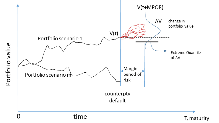
Figure 1: Change in portfolio value as a distribution (or a nested sample) for a single sample path over the Margin Period of Risk.

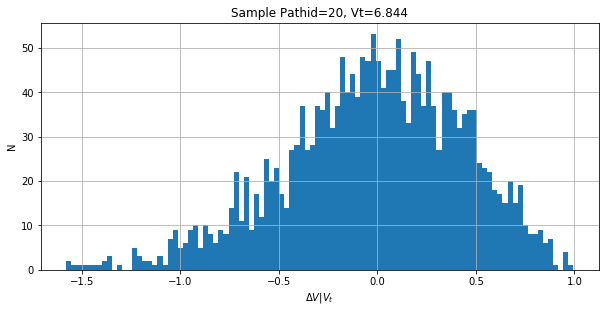
(a) $\Delta V$ samples for the Call Combination at time t=0.64 years

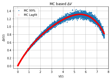
(b) Conditional 99% quantiles of $\Delta V$ given $V$ represented by blue dots and the corresponding polynomial regressed values shown as red curve.

Figure 2: Nested Monte-Carlo approach to estimate the Dynamic Initial Margin for the Call Combination.

Figure 2(a) shows the samples for $\Delta V_{t}^{\delta,f,\mathcal{M}}(\omega)$ for $N_{I}=1000$ inner samples, for a representative outer sample path (pathid 20) at time $t=0.64$ years. The portfolio value at that time for that outer path was $V_{t}(\omega)=6.844$. Figure 2(b) shows the corresponding 99% quantiles of $\Delta V$ over the entire cross section of the outer paths at the same time $t=0.64$ years - the conditional quantiles $Q_{\alpha}(\Delta V|V)$.

4 Nonnested Monte-Carlo: Cross-sectional Moment-Matching Methods

Due to the high computational requirements for simulation and valuation, it is rarely possible to spawn nested simulations for inner portfolio scenarios as required for the Nested MC type estimators, in particular for complex and/or large portfolios. Often, it is only possible to obtain several independent runs of the portfolio scenarios. Thus, methods such as Gaussian Least Square Monte-Carlo (GLSMC) and Johnson Least Square Monte-Carlo (JLSMC) [9, 3] are used to extract information about the distribution of the portfolio value change only from such outer simulations.

The data usually available from outer simulations is illustrated in Figure 3.

Figure 3: Change in portfolio values from outer simulations is used to estimate properties of the distribution $\Delta V$.

4.1 Moment-Matching Methods: GLSMC and JLSMC

Moment-Matching Least Square Monte Carlo methods can be outlined as follows:

• Generate $M$ portfolio scenarios (outer simulations) corresponding to the $k$ underlying assets, given the various risk factors and correlations from time $0$ till maturity $T$.

• Define the appropriate change in portfolio value corresponding to sample path $m$ as,

  $$\Delta V_{m}(t,\delta)=V_{m}(t+\delta)+\mathrm{DCF}_{m}(t,t+\delta)-V_{m}(t)$$ (6)

  where $V_{m}$ is the pathwise portfolio value in scenario $m$, and $\mathrm{DCF}_{m}$ is the value of the fully or partially included net cashflow between the counterparties from time $t$ to $t+\delta$.

• Based on the distribution(s) to be fitted, compute the first four raw sample moments $\Delta V_{m},$ $(\Delta V_{m})^{2}$, ($\Delta V_{m})^{3}$, $(\Delta V_{m})^{4}$ (for Johnson) or the first two raw sample moments $\Delta V_{m}$, $(\Delta V_{m})^{2}$ (for Gaussian) that will be used to estimate the actual raw moments.

• Accordingly estimate the first four raw moments, $r_{1},r_{2},r_{3},r_{4}$, or first two raw moments $r_{1},r_{2},$ as a function of the underlying states $\mathbf{X}_{t}$ or the portfolio value $V_{t}$ (or other regressors $\mathbf{R}_{t}$), by a suitable parameteric function such as polynomial regression,

  $$r_{i} = f(\bm{\beta},\mathbf{X})\approx E[(\Delta V)^{i}|\mathbf{X}_{t}=\mathbf{X}]$$

  or

  $$r_{i} = f(\bm{\beta},V)\approx E[(\Delta V)^{i}|V_{t}=V]$$

  where $\bm{\beta}$ is a vector of polynomial regression coefficients and $i=1,2,3,4$.

• GLSMC [3]: The estimated raw moments $r_{1},r_{2}$ can be used to approximate the mean and variance of the distribution $\Delta V_{t}$ ( portfolio value change of interest during MPoR) for an assumed normal distribution of $\Delta V_{t}$. The normal distribution with the estimated mean and variance is then used to estimate the conditional quantile.

• JLSMC [9]: The estimated first four raw moments $r_{1},r_{2},r_{3},r_{4}$ can be used to fit an appropriate Johnson’s distribution via Moment Matching method [5] with (approximately) these first four moments. The so obtained Johnson’s distribution is then used to estimate the conditional quantile.

An example of raw moments from the portfolio value change and the corresponding regressed moments with portfolio value $V_{t}$ via polynomial regression for the first four moments for Call Combination instrument is shown in Figure 4. Furthermore, the central moments obtained from these raw moments above (used for both GLSMC and JLSMC) were compared with those obtained from Nested Monte-Carlo method with $N_{I}=1000$ inner simulation paths for the same instrument. The comparison is shown in Figure 5 and the central moments obtained via regressed raw moments are seen to be in good agreement with the Nested MC.

A detailed procedure and the settings used for JLSMC is presented in [9] and is not repeated here for the sake of brevity. However, it is noted here that the moment matching algorithm [5] originally designed for smaller sets of observations is quite involved. Therefore the total number of given sets of moments that must be fit via the Johnson moment matching algorithm is equal to the number of outer simulation paths, $N_{O}=100,000$ at each time-step where Value at Risk is required. This poses a heavy computational burden in the absence of additional redesign and parallelization of the moment matching algorithm. Hence in order to reduce the computational load and obtain results with comparable accuracy, only moments at select values of the outer simulation values, either certain values of the underlying risk factors $\mathbf{X}_{t}$ or certain quantiles of the portfolio values $V_{t}$ at time $t$ are used for moment matching. Let $v_{j}=Q_{j/N}(V_{t}),j=0,\cdots,N$ be the $j/N$th quantile of the samples $V_{t}$ at time $t$ and

$$r^{i}_{j} =f_{i}(\bm{\beta},v_{j}),i=1,2,3,4$$

or

$$r^{i}_{j} =f_{i}(\bm{\beta},x_{j}),i=1,2,3,4$$

be the corresponding raw moments obtained via parameteric regression at the specific values of $V_{t}$ or $\mathbf{X}_{t}$. The parameters of the corresponding Johnson’s distribution obtained by the moment matching procedure are given by,

$$\mathtt{xi(j),lambda(j),delta(j),gamma(j),type(j)}=\mathtt{MomentMatching(r^{1}(j),r^{2}(j),r^{3}(j),r^{4}(j))}$$

where $\mathtt{xi(j),lambda(j),delta(j),gamma(j)}=\xi_{j},\lambda_{j},\delta_{j},\gamma_{j}$ are the parameters of the Johnsons distribution, and $\mathtt{type(j)}$ represents the type or family of the distribution. The pdf of Johnson’s distributions belonging to different families is given by [6, 9]:

• $S_{L}$ family,

  $$p(y)=\frac{\delta}{\sqrt{2\pi}}\frac{1}{y}\exp\left\{-\frac{1}{2}[\gamma+\delta\log(y)]^{2}\right\},\xi<X<\infty$$ (7)

• $S_{B}$ family,

  $$p(y)=\frac{\delta}{\sqrt{2\pi}}\frac{1-y}{y}\exp\left\{-\frac{1}{2}[\gamma+\delta\log(y/(1-y))]^{2}\right\},\xi<X<\xi+\lambda$$ (8)

• $S_{U}$ family,

  $$p(y)=\frac{\delta}{\sqrt{2\pi}}\frac{1}{\sqrt{y^{2}+1}}\exp\left\{-\frac{1}{2}[\gamma+\delta\log(y+\sqrt{Y^{2}+1})]^{2}\right\},-\infty<X<\infty$$ (9)

for $y=\frac{X-\xi}{\lambda}$.

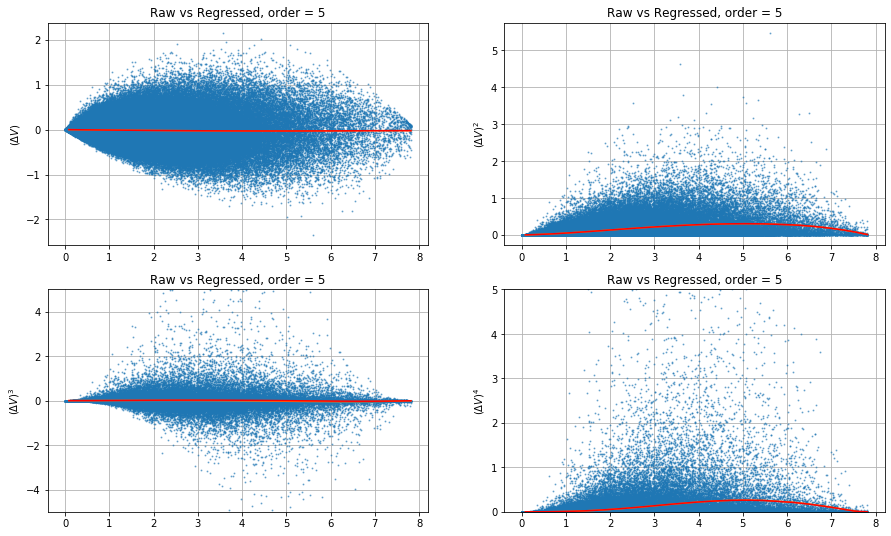
Figure 4: Polynomial regression of the first four raw-moments of the portfolio value change. Plotted over $V_{t}$.

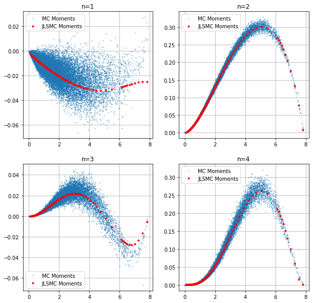
Figure 5: Comparison of the central moments computed from Nested Monte-Carlo simulation (blue dots) with those computed from regressed raw moments (red dots). Plotted over $V_{t}$

Interest Rate(IR) swap example: The above methods were compared for a realistic IR swap example, with one party making annual fixed rate payments with the counterparty making quarterly floating rate payments over a 15 year period. Here Party A pays floating rate with a constant spread of 0.9 % every 3 months over the current floating interest rate (LIBOR/PRIME etc). Party B pays fixed annual rate of 4.5 % every year based on the interest rate agreed at the start of the contract. The outstanding notational varies from 36.2 million dollars in the first year to 63.2 million dollars at the end of year 15. The Margin Period of Risk is set to 10 business days or 0.04 years, with a total of 375 intervals until maturity. The interest rate and risk factors were simulated following G1++ process and a sample path for cashflows, portfolio values and the risk factors is shown for a sample scenario in Figure 6.

Figure 6: Sample scenario of Interest Rate Swap with the portfolio value, accumulated fixed and floating cashflows and cashflows within MPoR. Plotted over time.

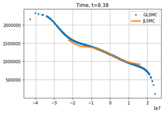
Figure 7: Comparison of Conditional quantiles at $\alpha=0.01$ obtained via GLSMC and JLSMC. The range of the JLSMC curve is smaller as only the quantiles 1 through 99 of values of $V_{t}$ at time $t=8.38$ were considered for moment matching and for $\Delta V$ quantile estimation. Plotted over $V_{t}$.

The conditional 1% quantiles obtained via GLSMC and JLSMC at time $t=8.38$ years are compared in Figure 7 and are found to be in good agreement. The GLSMC method is implemented over the entire cross-section of the outer paths, whereas the JLSMC method, as discussed earlier, was implemented at specific quantiles 1 through 99 of the values of $V_{t}$.

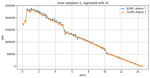
(a) Comparison of time evolution of DIM obtained via GLSMC and JLSMC with MPoR cashflows.

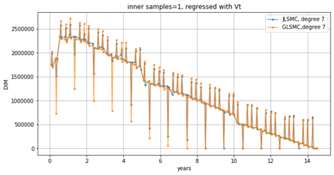
(b) Comparison of time evolution of DIM obtained via GLSMC and JLSMC without MPoR cashflows.

Figure 8: Time Evolution of DIMs for the IR Swap with moments regressed via Laguerre polynomials of degree 7.

Finally the time evolution of DIM for the same instrument over the entire 15 year period as defined in Equation (5) was compared for GLSMC and JLSMC. The results are shown in Figure 8 where the first four moments were regressed with Laguerre polynomials of degree seven. On the left, cashflows during MPoR are included in the change of value, on the right, MPoR cashflows are not included. It can be seen that not assuming that all cashflows are paid can make the margin requirements much more spiky. The results for the different methods are seen to be in good agreement with each other.

4.2 Further Analysis: JLSMC Moment Regression

We present another instrument, namely a cross currency FX-Call option in order to highlight the differences in the results obtained via the GLSMC and JLSMC methods. The Black-Scholes FX Call is simulated and priced with a constant domestic risk-free rate $r_{d}=0.08$, and a constant foreign rate of $r_{f}=0.02$ along with FX rate volatility of $\sigma=0.3$. The current spot FX rate is $S_{0}=100.0$. The option has maturity $T=1.0$ year and strike $K=105.0$. Similar to the other examples, the margin period of risk is fixed at $0.04$ years, with 25 MPoR intervals till maturity.

An algorithm to fit an appropriate Johnson’s distribution (Sl - logarithmic, Sb - bounded, Su -unbounded and Sn - normal) given the first four raw or central moments is presented in [5]. Raw moments are estimated by independent polynomial regression on the first four powers of the change in portfolio values as shown in Figure 4.

Johnson’s analysis of the types of distributions [6] also outlines the constraints for various moments, under which a valid distribution can be found. The relationship between Skew ($\beta_{1}$) and Kurtosis ($\beta_{2}$) requires that $\beta_{2}\geq\beta_{1}+1$. However, since the moments are regressed independently without imposing any joint constraints, there is no guarantee that relationship between Skew and Kurtosis will be satisfied everywhere when the regressed form of the moments is used. In fact, it can be seen that in some examples under some regression models, the Skew-Kurtosis relationship fails to hold at some points, and therefore one is unable to find a distribution that matches the moments, as shown in Figure 9. This is elaborated further in the following subsection.

4.2.1 Polynomial Moment Regression

The Skew vs Kurtosis obtained from the regressed raw moments at a single time is shown in Figure 9. Each data point corresponds to a unique path with a portfolio value $V_{m}(t)$ and its corresponding portfolio value change $\Delta V_{m}$. For simplicity only equally spaced quantiles from 0.01 to 0.99 of $V(t)$ are shown. The darker colors indicate lower quantiles closer to 0.01 and lighter colors indicate higher quantiles closer to 0.99, along with the line $\beta_{2}=\beta_{1}+1$. The data points where the condition is satisfied appear below that line and those that do not satisfy the constraint, appear above the $\beta_{2}=\beta_{1}+1$ line (the $\beta_{2}$ axis is reversed).

In the standard implementation of the moment-matching algorithm [5, 7], the data points not satisfying the relationship are discarded or just replaced by normal distribution with the given mean and variance only (first and second moments only) thus essentially reverting to the procedure for GLSMC in that case.

The results of the time evolution of DIM for the FX option is shown in Figure 10. It can be seen that although various methods agree well for the IR swap example (Figure 8), they deviate from each other for the FX option.

• This strongly indicates that different instruments have their own characteristic distributions for $\Delta V(t)|\mathcal{F}_{t}$ and hence cannot be approximated by normal distribution alone with the given mean and variance as in the GLSMC method. This also shows that a more accurate characterization of the distributions is needed, as in the JLSMC method.

• As mentioned earlier, when the Skew-Kurtosis relationship is not satisfied for the regressed moments, either the point is discarded or only a normal distribution matching only two moments is used. For the FX option, with the given polynomial regression, more data points violate the Skew-Kurtosis relationship at later times $t$. As those points are modeled by normal distributions rather than more expressive distributions, the estimated trends for DIM by JLSMC converge to that of GLSMC for such later times $t$ as as shown in Figure 10(a), which is clearly an artifact of the standard implementation.

Polynomial Regression Correction: To avoid that data points are discarded or only represented by normal distributions, it is possible to map the invalid Skew and Kurtosis value pairs to the closest Skew and Kurtosis value pair that does not violate the relationship and use the corresponding Johnson distribution. This is illustrated in Figure 9 where the data points above the $\beta_{2}=\beta_{1}+1$ line are projected onto the line in a (orthogonal) least-square sense as indicated by the red points. This ad-hoc method provides a better approximation of the distribution via a valid Johnson’s distribution instead via a normal distribution. In addition, a better model with a higher order polynomial regression or better regresion techniques such as ensemble learning via Random Forest might mitigate the issue with fewer data points violating the moment constraints. The time evolution of DIM with the proposed moment corrections is shown in Figure 10(b).

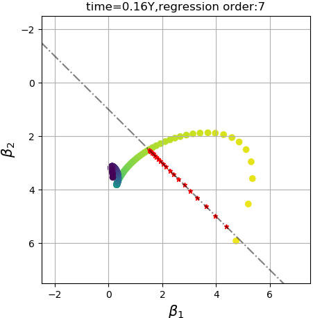
(a) The skew-kurtosis relationship.

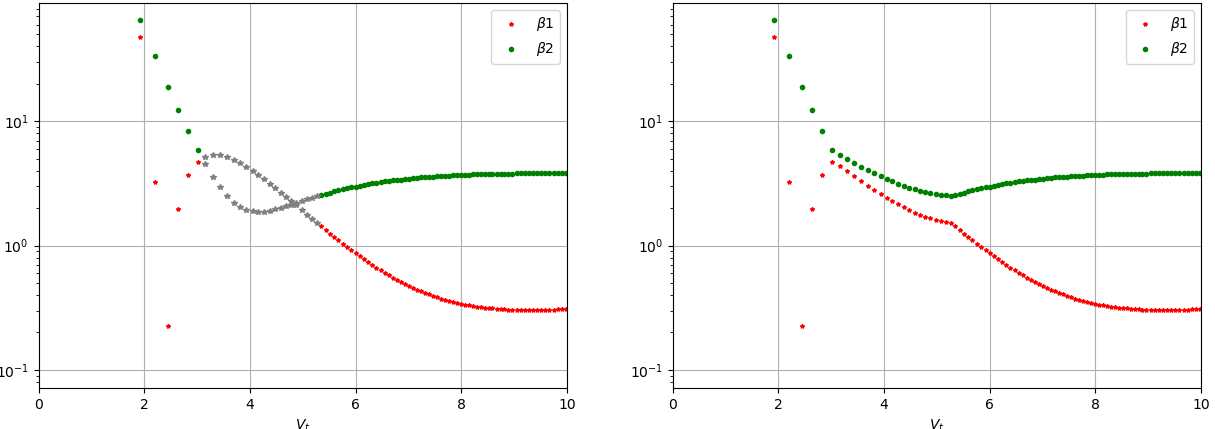
Figure 9: Skew-Kurtosis obtained from independently regressed moments is shown at selected quantiles (1 through 99) of $V_{t}$ (outer simulation) at time $t=0.16$ years. (Top) The datapoints that lie above $\beta_{2}=\beta_{1}+1$ (dotted line) violate the skew-kurtosis relationship and hence do not correspond to a valid distribution. (Bottom) Corresponding raw $\beta_{1}$ and $\beta_{2}$ against $V_{t}$ for the same time. (Bottom-Left) The gray datapoints denote those violating the relationship, (Bottom-Right) The moment-corrected data points.

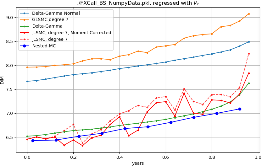
(a) Comparison of time evolution of DIM obtained via GLSMC and JLSMC with polynomial regression of order 7 (with and without moment correction) for the FX option.

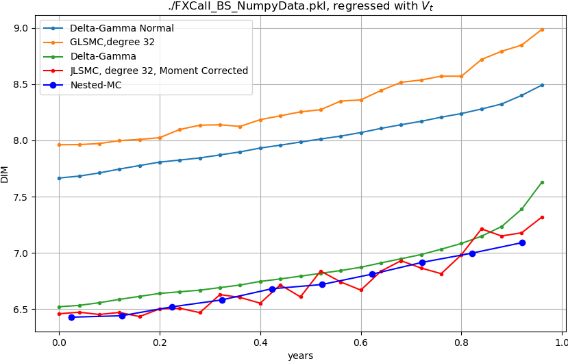
(b) Comparison of time evolution of DIM obtained via GLSMC and JLSMC for the FX option with moment correction and polynomial order 32.

Figure 10: Time Evolution of DIM for FX options with and without moment correction.

5 Nonnested Monte-Carlo: (Conditional) Quantile Regression

Conditional quantile regression [8] can be used to estimate population quantiles based on observations of a dataset $(\mathbf{C}_{i},y_{i})$ where $\mathbf{C}_{i}$ for each $i$ is a vector of covariates or features and $y_{i}$ is the quantity of interest (for instance, low birth weight or CEO compensation depending on maternal or firm characteristics, respectively, in two examples in [8]). Based on the vector $\mathbf{R}_{i}$ of covariates one regresses against, one estimates $q_{\alpha}(Y|\mathbf{R})$. The quantile regression procedure along with elicitability criteria for loss functions was used to extract conditional VaR and Expected Shortfall (ES) for XVA applications in [1].

We will use conditional quantile regression [8] as follows: Assuming that we have given ($r$-dimensional) samples $\mathbf{R}_{i}$ of regressors (chosen from a larger set of possible features) and samples $Y_{i}$ from the (one-dimensional) conditional distribution to be analyzed, the function $f_{\alpha}(\mathbf{R})$ is characterized as the function from an appropriately parametrized set of functions that minimizes the loss function

$$L_{\alpha}=\sum_{i}\rho_{\alpha}(Y_{i}-f_{\alpha}(\mathbf{R}_{i}))$$ (10)

with

$$\rho_{\alpha}(x)=\left\{\begin{array}[]{ccc}\alpha x&\mbox{ if }x\geq 0\\ (\alpha-1)x&\mbox{ if }x<0\end{array}\right..$$ (11)

$f_{\alpha}$ defined by $\operatorname*{arg\,min}L_{\alpha}$ then estimates the conditional quantile $q_{\alpha}(Y|\mathbf{R})$. [8] consider parametric functions $\mu(\mathbf{R},\beta)$ and in particular, functions that depend linearly on the parameters $\beta$. In their case, the optimal parameters can then be computed by linear programming. Here, we will apply conditional quantile regression both in the linear and nonlinear approximation context.

In our application, the conditional target distribution is the one of the portfolio value change $Y_{m}=\Delta V_{m}$ from time $t$ to time $t+\delta$ given some regressors or the complete Markovian state. The covariates that can be used have to be measurable as of time $t$. Assuming that the portfolio value can be exactly or approximately be considered Markovian in terms of current risk factor values $\mathbf{X}_{t}$ and extra state $\mathbf{U}_{t}$, $\mathbf{X}_{t}$ and $\mathbf{U}_{t}$ should contain all necessary information. Computing conditional quantiles conditional on the full state might be too expensive and thus, a smaller set of covariates might be used, such as the portfolio value $V_{t}$ and some “most important risk factors”.

In our machine and deep learning setting, we thus numerically minimize the loss function given above within an appropriate set of functions depending on the chosen regressors.

It is important to be parsimonious in the selection of the model and the number of free parameters, since with sufficient number of free parameters (and if there is only one value of $\Delta V_{m}$ for each $\mathbf{R}_{m}$), it is possible to learn each $\Delta V_{m}$ for each $\mathbf{R}_{m}$. A simple polynomial regression or a sufficiently simple neural network can strike a balance between a reasonably smooth approximation of the quantiles and achieving a local minimum for the loss function.

Figure 11 shows results of quantile regression for $dV|V$ with RF-LightGBM (upper panel) and DNN (lower panel). In the body of the $V_{t}$ distribution, results seems to mostly agree (with DNN giving a smoother results rather than the step wise curve coming from RF-LightGBM). For larger $V_{t}$, the behavior seems to be somewhat but not completely different.

Similarly as in least square regression, assuming that one tries to determine a quantile function as a linear combination of given functions of given features, there are faster deterministic numerical linear algebra methods available rather than resorting to generic optimization methods - linear least squares by SVD (in least square regression) and linear programming (for quantile regression). Once one no longer operates in the space of linear combinations of given functions, one needs to apply more generic and general numerical optimization techniques such as (stochastic) gradient descent or similar variants, both for least square regression and quantile regression.

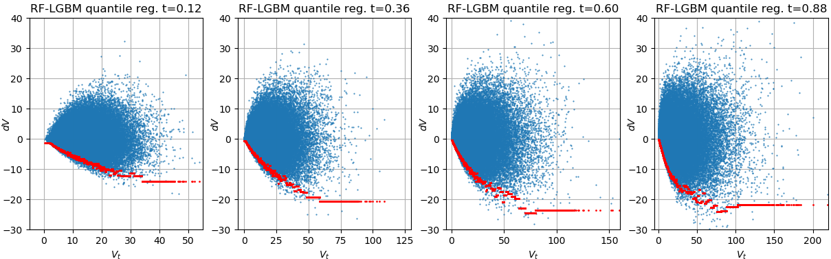
(a) Quantile regression via RandomForest-LightGBM on clean portfolio changes at various times.

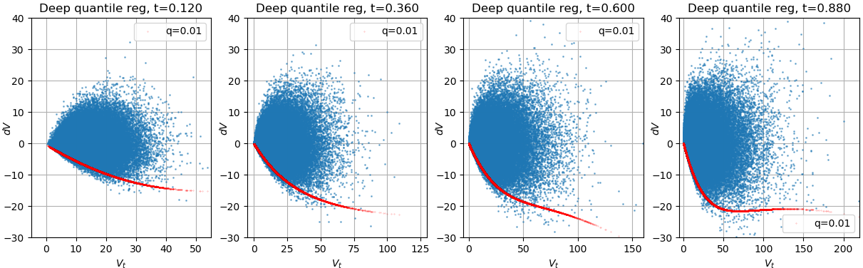
(b) Quantile regression via Deep Neural Networks on clean portfolio changes at various times.

Figure 11: Quantile regression performed on the clean change in portfolio values for the given outer portfolio scenarios for FX option instrument.

Figure 12 compares GLSMC, JLSMC, and Quantile Regression methods for the FX option (upper panel) and IR swap (lower panel). For the FX option, JLSMC and Quantile Regression seem to mostly agree, differing somewhat in smoothness (and looking similar to the earlier Nested MC results) while GLSMC gives materially different (and larger) values. For IR swap, all give broadly similar results.

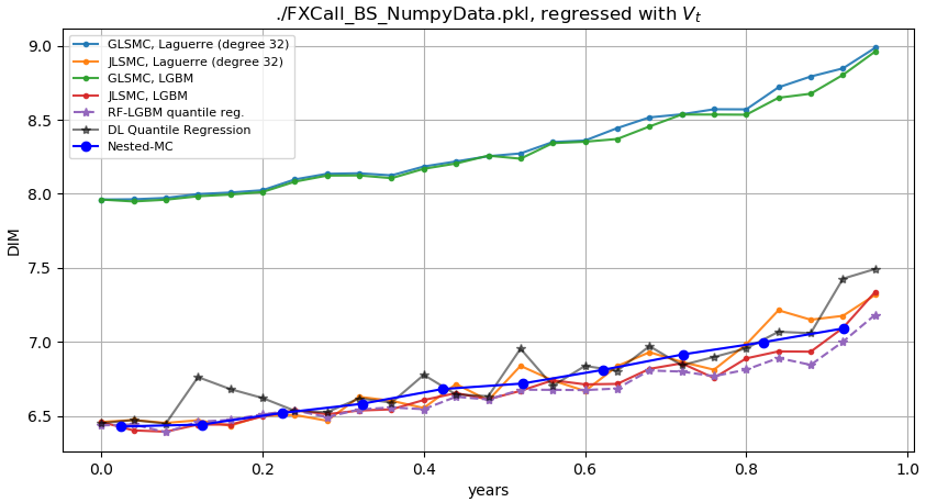
(a) Comparison of various methods for the time evolution of DIM for FX option instrument.

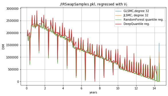
(b) Comparison of various methods of the time evolution of DIM for IR swap instrument.

Figure 12: Comparison of time-evolution of DIM for the FX option and IR swap instruments.

6 Nonnested Monte-Carlo but Given Sensitivities

Another technique to estimate the change in portfolio values over MPoR is to use portfolio sensitivities if available. The distribution of the return of the underlying risk factors can be combined with the portfolio sensitivies, specifically the first and second derivatives (portfolio Delta and Gamma) to obtain a good approximation of the distribution of the change in portfolio values over MPoR.

Let $\mathbf{S}(t)=(S_{1}(t),\cdots,S_{k}(t))$ be the values of the $k$ underliers that constitute the given portfolio and let $\mathbf{R}(t)=(\Delta S_{1}/S_{1},\cdots,\Delta S_{k}/S_{k})$ be the corresponding vector of asset returns where $\Delta S_{i}(t)=(S_{i}(t+\Delta t)-S(t))$. The second-order approximation of the change in the value of portfolio can be written in terms of the sensitivities as [10, 2],

$$\Delta V\approx\bm{\delta}_{\$}\mathbf{R}+\frac{1}{2}\mathbf{R}^{T}\mathbf{\Gamma}_{\$}\mathbf{R}$$ (12)

where,

$$\bm{\delta}_{\$} = (\delta_{1}^{\$},\delta_{2}^{\$},\cdots,\delta_{k}^{\$})^{T}$$ (13)

$$\delta_{i}^{\$} = \frac{\partial V}{\partial S_{i}}\times S_{i}$$ (14)

$$\mathbf{\Gamma}_{\$} = (\gamma_{ij}^{\$})$$ (15)

$$\gamma_{ij}^{\$} = \frac{\partial^{2}V}{\partial S_{i}\partial S_{j}}\times S_{i}\times S_{j}$$ (16)

where $V$ is the value of the portfolio corresponding to the value of the underliers. For a single underlier, the above equation can be written as,

$$\Delta V\approx\delta^{\$}R+\frac{1}{2}\gamma^{\$}R^{2}$$ (17)

for corresponding single asset return $R$.

6.1 Delta-Gamma Normal

As a first approximation, the change in portfolio values can be considered to be normally distributed, with mean and variance obtained from Eq. (17). Here the discounted asset return $R$, is assumed to be normally distributed with mean zero and variance $\Omega=\sigma^{2}$, (i.e) $R\sim\mathscr{N}(0,\Omega)$.

$$\Omega_{h} =\sigma^{2}\Delta t$$

$$\mathrm{E}(\Delta V) =\frac{1}{2}\mbox{tr}(\Gamma_{\$}\Omega_{h})$$

$$\mbox{Var}(\Delta V) =\frac{1}{2}\mbox{tr}[(\Gamma_{\$}\Omega_{h})^{2}]+\delta^{\prime}_{\$}\Omega_{h}\delta_{\$}$$

further with the approximation that $\Delta V$ follows a normal distribution, the corresponding $\alpha$th quantile of the distribution can be written as,

$$Q_{\alpha}(\Delta V|V)=z_{\alpha}\sqrt{(\mbox{Var}(\Delta V))}+\mathrm{E}(\Delta V)$$ (18)

where $z_{\alpha}$ is the $\alpha$th quantile of the standard normal distribution.

However this approximation, which could significantly deviate from the actual $\Delta V|V$ distribution, could lead to over-estimation or under-estimation of the margin requirements. This deviation due to the approximation is apparent from the actual sample distribution shown in Figure 2(a), which is skewed and could be heavy tailed dependending on value of the portfolio and the risk factors (Figure 13). Comparison of DIM obtained via this approximation against other methods for the call combination discussed earlier is shown in Figure 14(a) and Figure 14(b). Hence although the normal approximation of the $\Delta V|V$ distribution allows for rapid estimation of initial margin requirements, it may be not be suitable for complex portfolios or portfolios with more complex instruments.

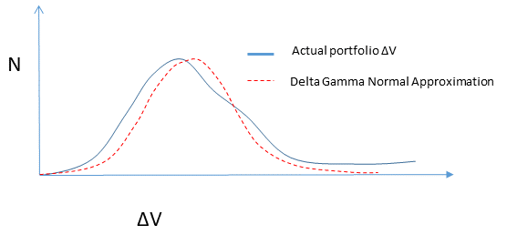
Figure 13: Approximation of $\Delta V$ distribution by Delta-Gamma Normal approach could lead to deviation from the actual $\Delta V$ distribution.

6.2 Delta-Gamma with Cornish-Fisher Cumulant Expansion

A further refinement of the previous method is to relate the quantiles of an empirical distribution to the quantiles of standard normal distribution via the higher order moments of the empirical distribution and the so called Cornish-Fisher expansion. Given the raw moments, and the corresponding central moments, ($cm_{1},cm_{2},cm_{3},cm_{4},cm_{5}$) from raw moments, compute the skew ($\kappa_{3}$), kurtosis ($\kappa_{4}$) and $\kappa_{5}=cm_{5}^{5}/cm_{2}^{5/2}$ from the central moments. Hence, the Delta-Gamma method approximates the quantiles of the portfolio value changes $\Delta V|V$ in terms of its raw moments and uses the Cornish-Fisher expansion to compute the $\alpha$th percentile of $\Delta V|V$.

$$Q_{\alpha}(\Delta V|\mathcal{F}_{t}) =z_{\alpha}+\kappa_{3}\frac{(z_{\alpha}^{2}-1)}{6}+\kappa_{4}\frac{z_{\alpha}^{3}-3z_{\alpha}}{24}$$

$$-\kappa_{3}^{2}\frac{(2z_{\alpha}^{3}-5z_{\alpha})}{36}+\kappa_{5}\frac{z_{\alpha}^{4}-6z_{\alpha}^{2}+3}{120}$$

$$-\kappa_{3}\kappa_{4}\frac{z_{\alpha}^{4}-5z_{\alpha}^{2}+2}{24}+\kappa_{3}^{3}\frac{12z_{\alpha}^{4}-53z_{\alpha}^{2}+17}{324}$$ (19)

where $z_{\alpha}$ is the $\alpha$th quantile of a standard normal distribution and $\kappa_{3},\kappa_{4},\kappa_{5}$ are the skew, kurtosis and higher order moments of the distribution. The Delta-Gamma approach approximates the above quantities from the corresponding portfolio sensitivities and asset returns over the MPoR.

Similar to the Delta Gamma Normal method, the discounted asset return is assumed to be normally distributed with mean zero and variance $\Omega$, (i.e) $R\sim\mathscr{N}(0,\Omega)$. The corresponding raw moments written as powers of $\Delta V$ in terms of $\delta^{\$}(=\delta),\gamma^{\$}(=\gamma),R$, and $\Omega$ are,

$$\Delta V = \delta^{\$}R+\frac{1}{2}\gamma R^{2}$$ (20)

$$\Delta V^{2} = \delta^{2}R^{2}+\frac{1}{4}\gamma^{2}R^{4}+\delta\gamma R^{3}$$ (21)

$$\Delta V^{3} = \delta^{3}R^{3}+\frac{1}{4}\delta\gamma^{2}R^{5}+\delta^{2}\gamma R^{4}+\frac{1}{8}\gamma^{3}R^{6}+\frac{1}{2}\delta\gamma^{2}R^{5}+\frac{1}{2}\delta^{2}\gamma R^{4}$$ (22)

$$= \delta^{3}R^{3}+\frac{3}{4}\delta\gamma^{2}R^{5}+\frac{3}{2}\delta^{2}\gamma R^{4}+\frac{1}{8}\gamma^{3}R^{6}$$

$$\Delta V^{4} = \delta^{4}R^{4}+\frac{3}{4}\delta^{2}\gamma^{2}R^{6}+\frac{3}{2}\delta^{3}\gamma R^{5}+\frac{1}{8}\delta\gamma^{3}R^{7}+\frac{3}{4}\delta^{2}\gamma^{2}R^{6}+\frac{1}{2}\delta^{3}\gamma R^{5}+\frac{3}{8}\delta\gamma^{3}R^{7}+\frac{1}{16}\gamma^{4}R^{8}$$ (23)

$$= \delta^{4}R^{4}+\frac{3}{2}\delta^{2}\gamma^{2}R^{6}+2\delta^{3}\gamma R^{5}+\frac{1}{2}\delta\gamma^{3}R^{7}+\frac{1}{16}\gamma^{4}R^{8}$$

$$\Delta V^{5} = \delta^{5}R^{5}+\frac{3}{2}\delta^{3}\gamma^{2}R^{7}+2\delta^{4}\gamma R^{6}+\frac{1}{2}\delta^{2}\gamma^{3}R^{8}+\frac{1}{16}\delta\gamma^{4}R^{9}$$ (24)

$$+\delta^{3}\gamma^{2}R^{7}+\frac{1}{2}\delta^{4}\gamma R^{6}+\frac{3}{4}\delta^{2}\gamma^{3}R^{8}+\frac{1}{4}\delta\gamma^{4}R^{9}+\frac{1}{32}\gamma^{5}R^{10}$$

$$= \delta^{5}R^{5}+\frac{5}{2}\delta^{3}\gamma^{2}R^{7}+\frac{5}{2}\delta^{4}\gamma R^{6}+\frac{5}{4}\delta^{2}\gamma^{3}R^{8}+\frac{5}{16}\delta\gamma^{4}R^{9}+\frac{1}{32}\gamma^{5}R^{10}$$

Using the first 10 moments of the normal distribution, the expectations of the above powers of $\Delta V$ can be written as

$$\mathrm{E}(\Delta V) =\frac{1}{2}\gamma\Omega$$

$$\mathrm{E}(\Delta V^{2}) =\delta^{2}\Omega+\frac{3}{4}\gamma^{2}\Omega^{2}$$

$$\mathrm{E}(\Delta V^{3}) =\frac{3}{2}\delta^{2}\gamma(3\Omega^{2})+\frac{1}{8}\gamma^{3}(15\Omega^{3})$$

$$\mathrm{E}(\Delta V^{4}) =\delta^{4}(3\Omega^{2})+\frac{3}{2}\delta^{2}\gamma^{2}(15\Omega^{3})+\frac{1}{16}\gamma^{4}(105\Omega^{4})$$

$$\mathrm{E}(\Delta V^{5}) =\frac{5}{2}\delta^{4}\gamma(15\Omega^{3})+\frac{5}{4}\delta^{2}\gamma^{3}(105\Omega^{4})+\frac{1}{32}\gamma^{5}(945\Omega^{5})$$

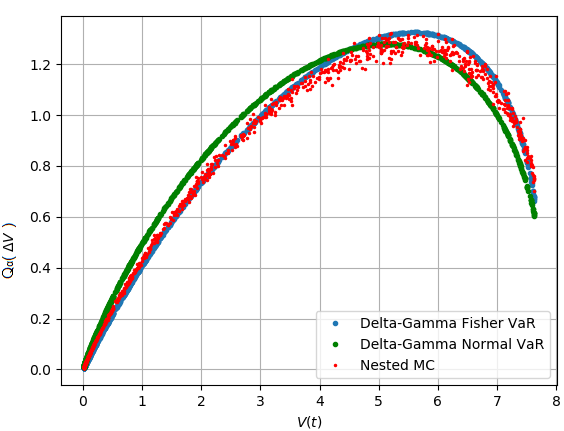
(a) Comparison of conditional quantiles at 1% for the call combination at a sample time $t$.

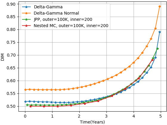
(b) Time Evolution of Dynamic Initial Margin

Figure 14: Comparison of Delta-Gamma approaches to estimate conditional quantiles and time-evolution of DIM for the call combination.

The central moments, ($cm_{1},cm_{2},cm_{3},cm_{4},cm_{5}$) from the above raw moments, the skew ($\kappa_{3}$), kurtosis ($\kappa_{4}$) and $\kappa_{5}=cm_{5}^{5}/cm_{2}^{5/2}$ derived from above terms are then used to determine the corresponding $\alpha$th quantile from Equation (19). The comparison of DIM and VaR estimates obtained via this method for the call combination discussed earlier is shown in Figure 14(a) and Figure 14(b), which is seen to be in much closer agreement with benchmark Nested-Monte Carlo method, while requiring far lower computational resources than the same. Hence the above method is suitable for instruments and portfolios with given analytical or approximate first and second order sensitivities.

7 Nested Monte-Carlo with Moderate Inner Samples

In the previous sections, the primary focus was on methods that only use outer simulations to estimate properties of the distribution of $\Delta V$, such as conditional quantile regression, quantile methods based on moment-matched distributions and regressed moments, or methods that use sensitivities and assumed distributions of underlying risk factors returns. However, these methods might benefit from refined estimates possible by limited inner simulations. The methods presented in this section below use the additional information from small and limited number of inner simulations to further refine their estimates for moment matching or quantile regression. Hence, the methods in this section could be thought of as a possible middle-ground between full-fledged Nested Monte-Carlo simulation with sufficiently many inner simulations requiring large computational resources on one side and efficient computational approaches such as moment-matching and quantile regression on the other.

7.1 Moment-Matching Methods

Based on the GLSMC and JLSMC methods presented in earlier sections, the moment-matching algorithms were applied to moment estimates of $\Delta V|V$ that used additional limited number of inner samples. The raw moments $(\Delta V_{m})^{i}$ for $i=1,2,3,4$ from a single outer path are replaced by $(1/N_{I})\sum_{j=1}^{N_{I}}(\Delta V_{jm})^{i}$ for $i=1,2,3,4$, where $N_{I}$ is the number of inner simulations for the outer portfolio scenario $m$. Here the number of inner simulations was chosen to be rather small as $N_{I}=50$ in order to limit the needed computational resources. The comparison of raw moments is shown in Figure 15 at a specific time $t=0.16$ years, across all the outer paths. It shows that additional inner samples decrease the variance of the raw moments. The time evolution of DIM obtained via GLSMC and JLSMC methods using these raw moments is shown in Figure 16. Although the time evolution obtained via GLSMC method has not changed much, as it depends only on the first two moments, the JLSMC method seems to exhibit a smoother time-evolution as it depends on and is sensitive to higher moments.

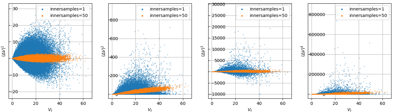
Figure 15: Refinement of first 4 raw moments at time 0.16 years with $N_{I}=50$ inner samples

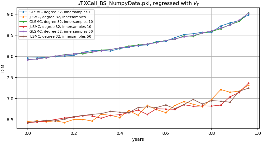
Figure 16: Comparison of the time-evolution of DIM between the GLSMC and JLSMC with different number of inner samples.

7.2 Johnson Percentile-Matching Method

The Johnson Percentile matching method fits a Sl, Su or Sb type Johnson distribution given a limited number of inner samples, based on a discriminant computed from particular percentiles of the inner samples data. The procedure is outlined in [11, 4]. In short, a fixed value $z(0<z<1)$ is chosen and the corresponding percentiles $P_{3z},P_{-3z},P_{z},P_{-z}$ of the standard normal distribution corresponding to the four points $\pm 3z$ and $\pm z$ are computed. The values of data points corresponding to the percentiles are then determined from the sample distribution as $Q_{P_{i}}(X)$, where $i=3z,z,-z,-3z$, as $x_{3z},x_{z},x_{-z},x_{-3z}$.

The value of the discriminant $d=mn/p^{2}$ is then used to select the type of Johnson distribution, where $p=x_{z}-x_{-z},m=x_{3z}-x_{z},n=x_{-z}-x_{-3z}$. The Su Johnson distribution is fit to the data if $d>1.001$, the Sb Johnson distribution chosen if $d<0.999$ and the Sl Johnson distribution is chosen if $0.999\leq d\leq 1.001$. This method provides closed form solution to the Johnson distribution parameters $\xi,\gamma,\delta$ and $\lambda$ in terms of the discriminant $d$ and $m,n$ hence requiring far lower computational resources than the moment matching algorithm.

The time evolution of DIM obtained via this method with a much reduced $N_{I}=200$ number of inner simulations is compared with Nested Monte-Carlo and Delta-Gamma approaches in Figure 14(b) and is seen to be in good agreement with the Nested Monte-Carlo approach.

7.3 Conditional Quantile Regression

The conditional quantile regression approach can also take advantage of additional inner samples. Similar to the other methods, samples from limited inner simulations were added to the training samples for quantile regression. A comparison of the time-evolution of DIM obtained via quantile regression with different number of inner samples is shown in Figure 17. Although the inner samples help refine the distribution, the time-evolution so obtained is still comparable in terms of accuracy and scale to that obtained with a single inner sample. This indicates that with sufficient number of outer samples (here $N_{O}=100,000$) the quantile regression procedure can be robust with respect to variations in inner distributions across the underlier at any given time or at different times. Comparing the results with a single inner sample versus the others, it seems that adding at least a few inner samples results in a somewhat smoother evolution of the DIM.

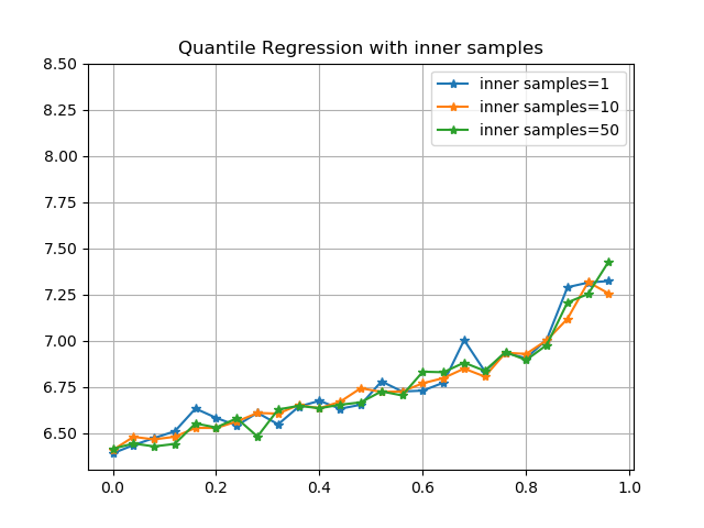
Figure 17: Comparison of the time-evolution of DIM via quantile regression with different number of inner samples.

7.4 Pseudo-Inner Samples

As the process of running nested inner simulations for a large number of outer simulations is computationally very expensive, an alternative method is to approximate inner simulations with available nearby outer simulation values around a neighborhood of $X_{t}$ or $V_{t}$. Hence under some circumstances, the values from outer simulations can be considered as proxy to samples from the actual distribution of portfolio values or pseudo-inner samples.

The distribution $(\Delta V|x_{t}=X_{t})$ is approximated by observations from portfolio scenario $m$, $\Delta V_{m}$ given by equation (6) such that $x^{(m)}_{t}\in\mathcal{B}_{\epsilon}(X_{t})$ or $V^{(m)}_{t}\in\mathcal{B}_{\epsilon_{1}}(V_{t})$ where the underlying asset or portfolio value is observed to be within a neighborhood $\mathcal{B}_{\epsilon}$ of $X_{t}$ or $V_{t}$. Figure 18 presents the time evolution of initial margin estimates obtained via limited number of pseudo-inner samples considered around around the neighborhood of $X_{t}$, for the Johnson’s Percentile matching method, along with regular inner-samples also implemented for the same method. It can be seed that both JPP with inner samples and JPP with pseudo-inner samples agree well with DIM obtained via Nested MC for the the combination call and FX call instruments. Additionally, the DIM obtained by estimating quantiles from the raw pseudo-samples is also presented, which is seen to be in good agreement with that obtained via Nested MC as well.

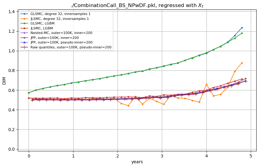
(a) Callcombination with pseudoinner samples.

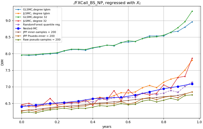
(b) FXcall with pseudoinner samples.

Figure 18: Comparison of the time-evolution of DIM with pseudo-inner samples.

8 Comparing Running Times and RMSE

We compare the methods presented above in terms of accuracy and speed. The Nested MC method is considered to be the benchmark for estimating the initial margin, and hence was used to measure the deviation in terms of RMSE accuracy. Additionally, the raw run time of the various methods was also recorded in order to compare multiple aspects of the methods. We ran the tests on a computer with 32GB of memory and Intel Core i7 processor with 8 cores. We did not spend much time optimizing the run time of the different methods or otherwise trying to ensure that the running times are very comparable so the listed running times should be taken only as indicative.

Table 3 presents the results for the FX call option with DIM computed for 25 times corresponding to various methods.

In terms of running time for this example, nested Monte Carlo, Johnson Moment Matching MC using LGBM regression and Johnson Percentile method take the longest, with DNN quantile regression being faster than those but slower than the quantile regressions with LGBM, LGBM quantile regressions take a medium amount of time, and the other methods take less than 100s with some taking less than 10s.

In terms of RMSE, the two quantile regressions using the LightGBM quantile regression were the most accurate while all other methods except the GLSMC and Delta-Gamma Normal methods were in the same order of magnitude with respect to RMSE.

The JPP method was implemented also with pseudo-samples, where a suitable Johnson distribution was fit to a collection from samples from adjacent outer simulations taken in-lieu of actual inner simulation samples. Since the percentile matching procedure has a convenient closed form solution, the procedure can be vectorized for multiple outer simulation values corresponding to different $V_{t}$s or $X_{t}$s, thus making for an efficient implementation for VaR or IM estimation. The DIM results obtained via this procedure, without the need for inner-samples, are compared against the previously studied methods. The run times are significantly faster along with improved accuracy, compared to traditional methods.

In addition, the same procedure can be repeated to estimate quantiles at each $V_{t}$ or $X_{t}$ from raw (pseudo-inner) samples without the need to fit a Johnson distribution. The results from this approach are also seen to outperform the traditional approaches both in terms of run-time and accuracy.

Table 2 presents results for a call combination with DIM computed for 125 times corresponding to various methods.

In terms of running time, we see similar results, nested Monte Carlo, Johnson Moment Matching MC using LGBM regression and Johnson Percentile method take the longest, LGBM quantile regressions take a medium amount of time, and the other methods take less than 100s with some taking less than 10s.

In terms of RMSE, using pseudo samples raw seems to give best accuracy, followed by Johnson Percentile methods with pseudo samples followed by Johnson Percentile method, quantile regressions using LGBM, and Johson MC Moment Matching using LGBM. On the other end of the spectrum, GLSMC methods, JLSMC regressing against $V_{t}$ (due to the non-uniqueness of the $V_{t}$ with respect to $X_{t}$) and Delta-Gamma-Normal methods give the least accurate results as measured by RMSE.

We see that even across these two relatively simple examples for which we can perform benchmarking with nested MC with large enough number of samples, a rather large variety of methods performs reasonably well in terms of RMSE accuracy and none performs uniformly best.

Method	RMSE	Time	Specification
Nested MC		2375s$\pm$ 43s	Outer=100K, Inner=2000
Raw Pseudo Samples	3.5e-5	16.2s$\pm$ 0.1s	Outer=100K, Pseudo-inner=200
Johnson Percentile	1.25e-04	2568s$\pm$ 18s	Outer=10K,Inner=200
Johnson Percentile with Pseudosamples	8.3e-05	27.1s$\pm$ 0.3	Outer=10K,Pseudo-inner=200, stride=10
Quantile Regression - LGBM($V_{t}$)	3.93e-4	269s$\pm$ 12s	Outer=100K, LightGBM, Reg with $V_{t}$
Quantile Regression - LGBM($X_{t}$)	6.96e-4	273s$\pm$ 13s	Outer=100K, LightGBM, Reg with $X_{t}$
Delta Gamma	7.33e-4	42.4s$\pm$ 0.9s	Outer=100K
Delta Gamma Normal	7.7e-3	35.4s$\pm$ 0.7s	Outer=100K
JLSMC - LGBM($X_{t}$)	4.86e-4	2412s$\pm$ 45s	Computed at 200 points in body and tails of $X_{t}$ Outer=100K, LightGBM, Reg with $X_{t}$
JLSMC - Lag($X_{t}$)	6.8e-3	63.4s$\pm$ 2.3s	Computed at 200 points in body and tails of $X_{t}$ Outer=100K, Laguerre, order 32, Reg with $X_{t}$
JLSMC - Lag($V_{t}$)	1.47e-2	58.3s$\pm$ 1.1s	Computed at 200 points in body and tails of $V_{t}$ Outer=100K, Laguerre, order 32, Reg with $V_{t}$
GLSMC - LGBM($X_{t}$)	8.94e-2	1220s$\pm$ 13s	Computed at 200 points in body and tails of $X_{t}$, Outer=100K, LightGBM, Reg with $X_{t}$
GLSMC - Lag($X_{t}$)	9.7e-2	33.7s$\pm$ 1.3s	Computed at 200 points in body and tails of $X_{t}$, Outer=100K, Laguerre, order 32, Reg with $X_{t}$
GLSMC - Lag($V_{t}$)	8.9e-2	30.1s$\pm$ 0.9s	Computed at 200 points in body and tails of $V_{t}$, Outer=100K, Laguerre, order 32, Reg with $V_{t}$

Table 2: Comparison of performance metrics of various methods for the Combination Call instrument
with 125 DIM instances

Method	RMSE	Time	Specification
Nested MC		438s$\pm$ 6s	Outer=100K, Inner=2000
Raw Pseudo Samples	6.69e-2	3.28s$\pm$0.2s	Outer=100K, Pseudo-inner=200
Johnson Percentile	2.74e-2	438s$\pm$ 9s	Outer=10K,Inner=200
Johnson Percentile with Pseudosamples	3.97e-02	5.97s$\pm$0.2	Outer=10K,Pseudo-inner=200, stride=10
Quantile Regression - LGBM($V_{t}$)	4.42e-3	53s$\pm$ 0.9s	Outer=100K, LightGBM, Reg with $V_{t}$
Quantile Regression - LGBM($X_{t}$)	4.26e-3	52.6s$\pm$0.8s	Outer=100K, LightGBM, Reg with $X_{t}$
Quantile Regression - DNN	4.7e-2	281.6s$\pm$ 15s	Outer=100K, Layers=4, Units=3, Batch-1024, Minimization Steps=20K
Delta Gamma	3.38e-2	10.6s$\pm$ 0.8s	Outer=100K
Delta Gamma Normal	1.72	9.5s$\pm$ 0.8s	Outer=100K
JLSMC - Lag($V_{t}$)	1.11e-2	12.82s$\pm$ 1.5s	Computed at 200 points in body and tails of $V_{t}$ Outer=100K, Laguerre, order 32, Reg with $V_{t}$
JLSMC - Lag($X_{t}$)	3.82e-2	13.4s$\pm$1.3s	Computed at 200 points in body and tails of $X_{t}$ Outer=100K, Laguerre, order 32, Reg with $X_{t}$
JLSMC - LGBM($X_{t}$)	4.13e-2	487s$\pm$7s	Computed at 200 points in body and tails of $X_{t}$ Outer=100K, LightGBM, Reg with $X_{t}$
GLSMC - Lag($V_{t}$)	2.54	7.4s$\pm$ 1.2s	Computed at 200 points in body and tails of $V_{t}$, Outer=100K, Laguerre, order 32, Reg with $V_{t}$
GLSMC - Lag($X_{t}$)	2.67	8.1s$\pm$0.9s	Computed at 200 points in body and tails of $X_{t}$, Outer=100K, Laguerre, order 32, Reg with $X_{t}$
GLSMC - LGBM($X_{t}$)	2.57	245s$\pm$4s	Computed at 200 points in body and tails of $X_{t}$, Outer=100K, LightGBM, Reg with $X_{t}$

Table 3: Comparison of performance metrics of various methods for the FX Call instrument
with 25 DIM instances

8.1 Discussion and Guidelines

It is illustrative to reflect on the requirements and constraints of each of these methods in light of the above results. The methods with pseudo samples outperform the traditional JLSMC and Quantile Regression methods in terms of accuracy and speed for these particular financial instruments with 1-dimensional risk-factors ($X_{t}$) and portfolio values ($V_{t}$). However, with multiple risk factors in higher dimensions the number of pseudo samples that can be borrowed from within a hyper-bin would be much sparser, thus leading to noisy estimates of quantiles. Secondly the number of hyper-bins that need to be considered grows rapidly with the dimensions thus forcing one to resort to $V_{t}$ based pseudo-samples for quantile estimation. Furthermore, even for 1-dimensional problems, it is necessary to have sufficient number of samples within a neighborhood of $V_{t}$ or $X_{t}$, in order to accurately capture the properties of the distribution. The number of active samples within any neighborhood of $V_{t}$ or $X_{t}$ becomes sparse with higher volatility and time horizon, again leading to noisy estimates. Hence, the pseudo-sample based methods are ideally suited for problems with rich outer-simulation data.

Methods with moment regression (JLSMC) give medium accuracy wherein it is necessary to have a good estimate of moment values, with methods and distributions that can fit higher moments typically performing better (JLSMC performing better than GLSMC).

Any inconsistencies in moment estimation leads to undefined distributions thus necessitating moment correction. Hence moment regression methods are particularly sensitive to the type of moment regression and the corresponding moment matching procedure. We also see that moment regression methods are relatively sensitive to the exact way how they are set up, thresholds, etc.

The quantile regression (LGBM quantile regression and Deep Quantile regression) procedures perform best with sufficient number of outer samples as they aim to minimize the quantile regression loss function. However the computational requirements grow with the number of available samples (outer-paths) while requiring sophisticated optimization frameworks. It is seen that LGBM quantile regression produces results comparable to pseudo-sample methods, as it employs a series of tree based optimizations and empirical estimation of quantiles in order to minimize the quantile loss function at the cost of longer runtime. On the other hand, the Deep Quantile regression procedure involves minimizing the quantile loss function via neural networks over several thousand minimization steps, which can become impractical for large number of DIM steps, unless the training of and optimization over the deep neural networks can be sped up substantially.

The objective of this study is to present the details and procedures of various methods used for estimation of fVaR and initial margin, along with with an objective evaluation of their accuracies and performance. The choice of method for a particular problem or financial instrument depends on variety of constraints and requirements as outlined in Table 1 and there is probably not a single method that can be applied for all financial instruments under all scenarios.

9 Conclusion

This paper discussed several methods to estimate future Values at Risk or margin requirements and their expected time-evolution (also called Dynamic Initial Margin), from simple options to more complex IR swaps. The methods analyzed in this paper are suited for instruments whose portfolio values are known or can be approximated well pathwise. In order to establish a baseline, the Nested MC method which is traditionally considered as a benchmark was used to validate other classical methods to estimate DIM. Under the current assumptions, the accuracy of these methods were studied taking into account necessary computational resources (Nested MC, moment matching, quantile regression, Johnson’s percentile-matching) and when first and second order sensitivities are available (Delta-Gamma methods). Furthermore, the differences between the estimated Dynamic Initial Margin curves were highlighted between the simpler GLSMC (Gaussian Least Square Monte-Carlo) and Delta-Gamma Normal and their more complex counterparts, JLSMC (Johnson Least Square Monte-Carlo) and Delta-Gamma methods. It was shown that standard moment regression methods can lead to violations of the skew-kurtosis relationship and that a simple correction procedure can lead to valid Johnson distributions and better performance. Conditional quantile regression with or without deep learning is a suitable technique with the help of an optimization framework, which however can demand computational resources for large number of DIM steps. The above methods were also compared in the presence of limited number of inner simulation runs to see whether such inner samples would further improve or refine the conditional quantile estimates. While all the methods benefit from available inner samples, it was seen that quantile regression tends to be more robust with sufficiently large number of outer simulation runs, even without additional inner samples. Finally the techniques where inner samples are necessary, such as Nested MC and Johnson’s Percentile matching, it is possible to replace them with pseudo-inner samples under specific conditions, for comparable performance and much faster runtimes where the results were demonstrated for FX call and combination call instruments.

10 Acknowledgement

The authors would like to thank Vijayan Nair for valuable discussions and comments regarding methods (in particular his suggestions to explore pseudo-sample approaches), presentation, and results, and Agus Sudjianto for supporting this research.

References

- [1] Claudio Albanese, Stephane Crepey, Rodney Hoskinson, and Bouazza Saadeddine. XVA analysis from the balance sheet. arXiv preprint arXiv:2009.00368, 2020.
- [2] Carol Alexander. Market Risk Analysis. Volume IV: Value-at-Risk Models. John Wiley & Sons, Ltd, 2008.
- [3] Peter Caspers, Paul Giltinan, Roland Lichters, and Nikolai Nowaczyk. Forecasting initial margin requirements - a model evaluation. 2017. Available at SSRN: https://ssrn.com/abstract=2911167 or http://dx.doi.org/10.2139/ssrn.2911167.
- [4] Florence George and K. M. Ramachandran. Estimation of parameters of Johnson’s system of distributions. Journal of Modern Applied Statistical Methods, 10(2):494–504, 2011.
- [5] I. Hill, R. Hill, and R. Holder. Algorithm AS 99: Fitting Johnson curves by moments. Journal of the royal statistical society. Series C (Applied statistics), 25(2):180–189, 1976.
- [6] N. L. Johnson. Systems of frequency curves generated by methods of translation. Biometrika, 36(1/2):149–176, 1949.
- [7] D. Jones. Johnson curve toolbox for Matlab: analysis of non-normal data using the Johnson family of distributions. 2014.
- [8] Roger Koenker and Kevin F. Hallock. Quantile regression. Journal of Economic Perspectives, 15(4):143–156, 2001.
- [9] Thomas McWalter, Joerg Kienitz, Nikolai Nowaczyk, Ralph Rudd, and Sarp Kaya Acar. Dynamic Initial Margin estimation based on quantiles of Johnson distributions. 2018. Also Available at SSRN: https://ssrn.com/abstract=3147811 or http://dx.doi.org/10.2139/ssrn.3147811.
- [10] Steven Shreve. Stochastic Calculus for Finance II, Continuous-Time Models. Springer-Verlag New York, 2004.
- [11] James F. Slifker and Samuel S. Shapiro. The Johnson system: Selection and parameter estimation. Technometrics, 22(2):239–246, 1980.