Cosmic Star-Formation History Measured at 1.4 GHz

Abstract

We matched the 1.4 GHz local luminosity functions of star-forming galaxies (SFGs) and active galactic nuclei to the 1.4 GHz differential source counts from $0.25\,\mu\mathrm{Jy}$ to 25 Jy using combinations of luminosity and density evolution. We present the most robust and complete local far-infrared (FIR)/radio luminosity correlation to date in a volume-limited sample of $\approx 4.3\times 10^{3}$ nearby SFGs, finding that it is very tight but distinctly sub-linear: $L_{\mathrm{FIR}}\propto L_{\mathrm{1.4\,GHz}}^{0.85}$. If the local FIR/radio correlation does not evolve, the evolving 1.4 GHz luminosity function of SFGs yields the evolving star-formation rate density (SFRD) $\psi(M_{\odot}\,\mathrm{year}^{-1}\,\mathrm{Mpc}^{-3}$) as a function of time since the big bang. The SFRD measured at 1.4 GHz grows rapidly at early times, peaks at “cosmic noon” when $t\approx 3\,\mathrm{Gyr}$ and $z\approx 2$, and subsequently decays with an $e$-folding time scale $\tau=3.2\,\mathrm{Gyr}$. This evolution is similar to, but somewhat stronger than, SFRD evolution estimated from UV and FIR data.

1 Introduction

Fundamental to our understanding of galaxy evolution, reionization of the universe, and heavy element production is an evolutionary timeline of the cosmic star formation rate density (SFRD). In the 1990s, it was first suggested that star-formation activity at redshift $z\sim 1$ dwarfed that at $z\sim 0$ (e.g. Songaila et al., 1994; Ellis et al., 1996; Lilly et al., 1996). In the decades since, star-forming galaxies have been detected out to increasing redshifts, most recently $z\gtrsim 10$ (e.g. Coe et al., 2013; Oesch et al., 2016), well within the reionization era. Compilations of SFR measurements made at various redshifts informs our understanding of SFRD evolution (see Hopkins & Beacom, 2006; Madau & Dickinson, 2014, for reviews of the topic). Virtually all SFR diagnostics are sensitive to massive stars only; an initial mass function (IMF) must be assumed to tally the total stellar mass formed at a given time. Possible variations in the IMF within and among galaxies and redshifts remains a source of uncertainty.

Most extragalactic radio sources fainter than $S\approx 0.4\,\mathrm{mJy}$ at $1.4\,\mathrm{GHz}$ are distant star-forming galaxies (SFGs), while stronger sources are primarily radio galaxies or quasars powered by active galactic nuclei (AGNs) (Prandoni et al., 2001; Smolčić et al., 2008; Condon et al., 2012; Vernstrom et al., 2016). The 1.4 GHz continuum emission from SFGs is a combination of synchrotron radiation from electrons accelerated in the supernova remnants of short-lived ($\tau\leq 3\times 10^{7}\,\mathrm{yr}$) massive ($M>8M_{\odot}$) stars plus thermal bremsstrahlung from Hii regions ionized and heated by even more massive stars (Condon, 1992). The cosmic-ray electrons responsible for the synchrotron radiation dominating the 1.4 GHz continuum emission eventually diffuse throughout their host galaxy and cool on timescales $\tau_{\rm cool}\sim 5$ Myr (for a spiral galaxy that stopped forming stars after a single episode; Murphy et al., 2008). The combined lifetimes of such massive stars with the cooling timescale of cosmic-ray electrons are much less than the age of the universe, so the radio continuum luminosities of SFGs depend only on their current star-formation rates uncontaminated by older stellar populations. Although the radio continuum luminosity is only a tiny fraction of the total power emitted by massive stars, its tight correlation with the energetically dominant far-infrared (FIR) emission from dust heated by massive stars justifies the use of radio emission as a quantitative tracer of star formation in galaxies (Condon, 1992).

Stars with masses $M\gtrsim 8M_{\odot}$ emit primarily in the ultraviolet (UV) continuum. The rest frame wavelength range 1400 Å to 1700 Å is accessible to ground-based telescopes for galaxies with redshifts $z\gtrsim 1.4$, but the UV emission of nearby galaxies must be measured either at longer UV wavelengths or from space. The contribution from longer-lived ($\tau\sim 250$ Myr) radio-quiet stars increases at longer UV wavelengths. The biggest downside for UV emission as a tracer of the SFR is dust obscuration. At redshifts $z\sim 2$, dust attenuation measured via infrared/UV luminosity ratios $L_{\rm IR}/L_{\rm UV}$ implies that $>$80% of star formation is obscured (Reddy et al., 2012; Howell et al., 2010), resulting in a small UV contribution to the total SFRD.

The UV energy absorbed by dust grains is reemitted at mid-infrared (MIR) and far-infrared (FIR) wavelengths, making MIR and FIR luminosities practical SFR indicators (in the case of minimal contribution from diffuse dust). Although FIR ($42.5-122.5\,\mu\mathrm{m}$; Helou et al., 1988) dust extinction is low, the infrared spectrum (spanning $\lambda=8-1000\,\mu$m) of a galaxy is complex. The fraction of UV luminosity absorbed by dust depends on the metallicity and geometry of the dust distribution, and the dust emission at wavelengths longer than $\lambda\sim 100\,\mu$m in the source frame is powered primarily by evolved stars (e.g. Hirashita et al., 2003; Bendo et al., 2010). At MIR wavelengths, emission from warm dust is tightly correlated with star formation, but polycyclic aromatic hydrocarbons (PAHs) complicate the emission spectrum near $\lambda=8\,\mu$m and active galactic nuclei (AGNs) dilute these PAH features while also contributing significantly to the 24$\,\mu$m continuum emission. Luminous infrared galaxies (LIRGS) with $L_{\mathrm{IR}}>10^{11}L_{\odot}$ and ultra-luminous infrared galaxies (ULIRGS) with $L_{\mathrm{IR}}>10^{12}L_{\odot}$ are rare today but were responsible for most of the luminosity density during the $z\sim 2$ “cosmic noon” (Magnelli et al., 2011) when most stars were formed. The MIR emission due solely to star formation must be disentangled from the total MIR emission before converting to a SFR to ensure a correct result.

The cosmic history of star formation can be constrained by a combination of the 1.4 GHz local luminosity function and the differential numbers $n(S)dS$ of faint radio sources per steradian with flux densities between $S$ and $S+dS$. A very low 1.4 GHz detection limit $S=0.25\,\mu$Jy is needed to reach SFRs of evolving “normal” galaxies like the Milky Way: $5\,M_{\odot}\,\mathrm{yr}^{-1}$ at $z=2$, $12\,M_{\odot}\,\mathrm{yr}^{-1}$ at $z=3$, and $22\,M_{\odot}\,\mathrm{yr}^{-1}$ at $z=4$ (assuming a Salpeter IMF). Thus the top continuum science goal of the proposed Square Kilometre Array SKA1-MID is “Measuring the Star-formation History of the Universe” using the proposed “Ultra Deep Reference Survey” to count sources as faint as $S=0.25\,\mu\mathrm{Jy}$ in a solid angle $\Omega\approx 1\,\mathrm{deg}^{2}$ (Prandoni & Seymour, 2015). Recently Condon et al. (2019) measured the 1.4 GHz local (${z<0.1}$) radio luminosity functions of SFGs and AGNs from sources in the 1.4 GHz NRAO VLA Sky Survey (Condon et al., 1998, NVSS) cross-identified with 2MASX galaxies (Jarrett et al., 2000). Matthews et al. (2021) determined accurate 1.4 GHz brightness-weighted source counts $S^{2}n(S)$ over the eight decades of flux density between $S=0.25\,\mu\mathrm{Jy}$ and $S=25\,\mathrm{Jy}$ using the very sensitive $\nu=1.266\,\mathrm{GHz}$ MeerKAT DEEP2 sky image (Mauch et al., 2020) for sources counts below $S=2.5\,\mathrm{mJy}$, and the 1.4 GHz NVSS catalog above $S=2.5\,\mathrm{mJy}$ (see Matthews et al. (2021) for details).

In this paper we present the cosmic star-formation history derived from only (1) the 1.4 GHz local luminosity function, (2) the local volume-limited FIR/radio correlation, and (3) the 1.4 GHz counts of sources as faint as $S=0.25\,\mu\mathrm{Jy}$. We do not need to “stack” radio sources to achieve the required sensitivity, so we do not depend on a complete sample of optically selected galaxies with measured redshifts and do not discriminate against galaxies so obscured by dust that they drop out of optical samples. The faintest radio sources were detected statistically via their confusion $P(D)$ distribution, so we actually cannot optically identify them or measure their redshifts. Instead, their radio evolution is constrained entirely by matching features in the local luminosity function to features in the source counts. This independent approach complements the traditional methods reviewed by Madau & Dickinson (2014).

Section 2 reviews and updates the 1.4 GHz local luminosity functions of SFGs and AGNs derived from a spectroscopically complete sample of $\sim 10^{4}$ 2MASX (Jarrett et al., 2000) galaxies brighter than $k_{20fe}=+11.75$ at $\lambda=2.2\,\mu$m and stronger than $S=2.5\,\mathrm{mJy}$ at $\nu=1.4\,\mathrm{MHz}$. Basic equations relating the evolving $1.4\,\mathrm{GHz}$ luminosity functions and spectral-index distributions to the counts of distant sources in the flat $\Lambda$CDM universe are introduced in Section 3. The non-evolving model source counts are discussed in Section 4 to highlight the features that evolutionary models must have to fit the 1.4 GHz data. Models for the radio evolution of both AGNs and SFGs that successfully match their evolving luminosity functions to the 1.4 GHz source counts are presented in Section 5. We calculated an improved local FIR/radio correlation using a large volume-limited sample of SFGs in our 2MASX sample and found it to be a slightly nonlinear power law: $L_{\mathrm{FIR}}\propto L_{\mathrm{1.4\,GHz}}^{0.85}$. We used this local FIR/radio correlation to convert the evolving 1.4 GHz SFG luminosity functions into FIR star-formation rate densities (SFRDs) and to make an independent estimate of the cosmic history of star formation (Section 6). Section 7 summarizes and evaluates these results.

Absolute quantities were calculated for the flat $\Lambda$CDM universe with $H_{0}=70\,\mathrm{km\,s}^{-1}\mathrm{\,Mpc}^{-1}$ and $\Omega_{\mathrm{m}}=0.3$. Our spectral-index sign convention is $\alpha\equiv+d\,\ln S/d\,\ln\nu$. The Salpeter (1955) IMF was used to calculate total star-formation rates in terms of $M_{\odot}\,\mathrm{yr}^{-1}$. These rates should be multiplied by 0.61 for the Chabrier (2003) IMF or by 0.66 for the Kroupa (2001) IMF.

2 Local 1.4 GHz Luminosity Functions

The evolving spectral luminosity function $\rho(L_{\nu}|z)dL_{\nu}$ specifies the comoving number density of sources at redshift $z$ having absolute spectral luminosities $L_{\nu}$ to $L_{\nu}+dL_{\nu}$ at frequency $\nu$. The corresponding density of sources per decade of spectral luminosity is

$$\rho_{\mathrm{dex}}(L_{\nu}|z)=\ln(10)L_{\nu}\rho(L_{\nu}|z)~{}.$$ (1)

Sources with this luminosity function produce a comoving spectral power density per decade of luminosity

$$u_{\mathrm{dex}}(L_{\nu}|z)\equiv L_{\nu}\,\rho_{\mathrm{dex}}(L_{\nu}|z)~{}.$$ (2)

We call $u_{\mathrm{dex}}$ the energy-density function because spectral power density has the same dimensions as energy density (SI units $\mathrm{W\,Hz}^{-1}\mathrm{\,m}^{-3}=\mathrm{J\,m}^{-3}$). Astronomically practical units for $u_{\mathrm{dex}}$ are $\mathrm{W\,Hz}^{-1}\,\mathrm{dex}^{-1}\,\mathrm{Mpc}^{-3}$.

The local 1.4 GHz energy-density functions $u_{\mathrm{dex}}(L_{\nu}|0)$ of radio sources powered primarily by active galactic nuclei (AGNs) or by star-forming galaxies (SFGs) were determined separately (Condon et al., 2019) and are shown by the data points and error bars in Figure 1. These local 1.4 GHz energy-density functions were determined from a large sample ($N\sim 1\times 10^{4}$) of radio sources in the NVSS catalog covering $\Omega=7.016$ sr of sky and cross-identified with $\lambda=2.16\,\mu$m galaxies in the 2MASX. All 9517 sources have spectroscopic redshifts and radio sources powered primarily by AGNs were separated from those powered by SFGs using the following radio and infrared diagnostics: (1) an IRAS FIR/NVSS 1.4 GHz flux-density ratio $q<1.8$, (2) a FIR spectral index $\alpha(25\,\mu\mathrm{m},\,60\,\mu\mathrm{m})>-1.25$, (3) have WISE colors $(W1-W2)>0.8$ for $(W2-W3)\geq 3.1$ and $(W1-W2)>(W2-W3-1.82)/1.6$ for $(W2-W3)<3.1$, and (4) showed a radio morphology with multiple components (e.g. jets, lobes in the case of resolved NVSS sources). The median redshift (corrected for the local flow due to nearby galaxy clusters) is $\langle z\rangle\approx 0.02$ for the SFG sample ($N=6699$) and $\langle z\rangle\approx 0.04$ for the AGNs ($N=2763$). For further details on the derivation of these energy-density functions, we refer the reader to Condon et al. (2019). For computational convenience, we approximate the AGN energy-density function by

$$u_{\mathrm{dex}}(L_{\nu}|0)=\frac{C_{\mathrm{a}}L_{\nu}}{(L_{\nu}/L^{*}_{\mathrm{a}})^{\alpha}+(L_{\nu}/L^{*}_{\mathrm{a}})^{\beta}+(L_{\nu}/L_{\mathrm{min}})^{\gamma}}$$ (3)

with comoving density factor $C_{\mathrm{a}}=2.0\times 10^{-6}\,\mathrm{Mpc}^{-3}\allowbreak\,\mathrm{dex}^{-1}$, AGN high-luminosity turnover spectral luminosity $L^{*}_{\mathrm{a}}=2.0\times 10^{25}\,\mathrm{W\,Hz}^{-1}$, low-luminosity downturn luminosity $L_{\mathrm{min}}=1.0\times 10^{11}\,\mathrm{W\,Hz}^{-1}$, intermediate-luminosity power-law slope $\alpha=0.55$, high-luminosity power-law slope $\beta=1.9$, and low-luminosity downturn slope $\gamma=-0.25$. This function is shown by the red curve in Figure 1. Its parameters are highly correlated, so their values and their uncertainties have limited physical significance. However, the uncertainty of $\beta$ is especially large because there are few AGNs with $L_{\nu}>L^{*}_{\mathrm{a}}$ and redshifts $z<0.1$.

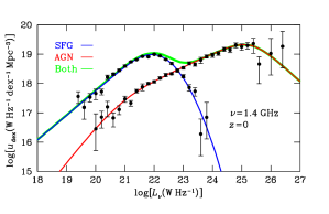
Figure 1: The measured local energy-density functions $u_{\mathrm{dex}}(L_{\nu}|0)$ at $\nu=1.4\,\mathrm{GHz}$ are shown by the black data points. The red curve plots the Equation 3 fit for AGNs, the blue curve plots Equation 4 for SFGs, and the wider green curve is the sum of both.

The tight FIR/radio correlation implies that the radio and FIR luminosity functions of SFGs should have similar functional forms, so we followed the standard form established by Saunders et al. (1990) for the $\lambda=60\,\mu\mathrm{m}$ luminosity function to write

$$u_{\mathrm{dex}}(L_{\nu}|0)=C_{\mathrm{s}}\biggl{(}\frac{L_{\nu}}{L^{*}_{\mathrm{s}}}\biggr{)}^{2-\alpha_{\mathrm{s}}}\hskip-5.69046pt\exp\biggl{[}-\frac{1}{2\sigma^{2}}\log^{2}\biggl{(}1+\frac{L_{\nu}}{L^{*}_{\mathrm{s}}}\biggr{)}\biggr{]}$$ (4)

with comoving density factor $C_{\mathrm{s}}=3.50\times 10^{-3}\,\mathrm{Mpc}^{-3}\allowbreak\,\mathrm{dex}^{-1}$, turnover spectral luminosity $L^{*}_{\mathrm{s}}=1.9\times 10^{21}\,\mathrm{W\,Hz}^{-1}$, $\alpha_{\mathrm{s}}=1.162$ for low-luminosity power-law slope $(2-\alpha_{\mathrm{s}})=+0.838$, and high-luminosity Gaussian taper with rms width $\sigma=0.558$. Our value of $L^{*}_{\mathrm{s}}$ is close to the $L_{\nu}=2.5\times 10^{21}\,\mathrm{W\,Hz}^{-1}$ 1.4 GHz spectral luminosity of the Milky Way (Berkhuijsen, 1984). The local energy-density function of SFGs is plotted as the blue curve in Figure 1, and the sum of the AGN and SFG local energy-density functions is indicated by the wider green curve.

The accessible volumes and hence numbers of galaxies with low 1.4 GHz luminosities used to calculate the local energy-density functions are limited primarily by the $S\approx 2.5\,\mathrm{mJy}$ sensitivity limit of the NVSS catalog, so the statistical uncertainties in these energy-density functions increase for AGNs below $L_{\nu}\sim 10^{21}\,\mathrm{W\,Hz}^{-1}$ and for SFGs below $L_{\nu}\sim 10^{20}\,\mathrm{W\,Hz}^{-1}$.

3 Basic Equations

The differential source count $n(S)dS$ is the number of sources per steradian with flux densities between $S$ and $S+dS$. Defining $\eta(S)d\log(S)$ as the number of sources per steradian per $\log(S)$ and substituting $dS=Sd\ln(S)=\ln(10)Sd\log(S)$ shows that $\ln(10)S^{2}n(S)=S\eta(S)$ is the flux density per steradian (a spectral brightness) per decade of flux density. Thus the Rayleigh-Jeans sky brightness temperature $dT_{\mathrm{b}}$ per decade of flux density contributed by sources is

$$\Biggl{[}\frac{d\,T_{\mathrm{b}}}{d\log(S)}\Biggr{]}=\Biggl{[}\frac{\ln(10)\,c^{2}}{2k_{\mathrm{B}}\nu^{2}}\Biggr{]}S^{2}n(S)~{},$$ (5)

where $k_{\mathrm{B}}\approx 1.38\times 10^{-23}\mathrm{\,J\,K}^{-1}$. We call $S^{2}n(S)$ the brightness-weighted differential source count to distinguish it from the traditional static-Euclidean weighted count $S^{5/2}n(S)$.

In a flat $\Lambda$CDM universe, the total brightness-weighted count at frequency $\nu$ of sources with spectral index $\alpha$ can be written as the integral of $u_{\mathrm{dex}}(L_{\nu}|z)$ over redshift (Condon & Matthews, 2018):

$$S^{2}n(S)=\frac{D_{H_{0}}}{4\pi\ln(10)}\int_{0}^{\infty}u_{\mathrm{dex}}(L_{\nu}|z)\biggl{[}\frac{(1+z)^{\alpha-1}}{E(z)}\biggr{]}\,dz~{},$$ (6)

where $D_{H_{0}}\equiv c/H_{0}$ is the Hubble distance, $L_{\nu}=4\pi D_{\mathrm{C}}^{2}(1+z)^{1-\alpha}S$, $D_{\mathrm{C}}$ is the comoving distance to the source, and $E(z)=[\Omega_{\mathrm{m}}(1+z)^{3}+\Omega_{\Lambda}+\Omega_{\mathrm{r}}(1+z)^{4}]^{1/2}$.

It is instructive to rewrite Equation 6 in terms of lookback time $t_{\mathrm{L}}(z)$ by substituting the relations (Condon & Matthews, 2018)

$$dD_{\mathrm{C}}=D_{H_{0}}\frac{dz}{E(z)}=(1+z)c\,dt_{\mathrm{L}}$$ (7)

to yield

$$S^{2}n(S)=\frac{c}{4\pi\ln(10)}\int_{0}^{t_{\mathrm{L}}(\infty)}u_{\mathrm{dex}}(L_{\nu}|z)(1+z)^{\alpha}dt_{\mathrm{L}}\,,$$ (8)

where $t_{\mathrm{L}}(z=\infty)\approx 0.964H_{0}^{-1}\approx 13.47\,\mathrm{Gyr}$ is the current age of the universe. Equation 8 shows that the sources in any narrow range $\Delta t_{\mathrm{L}}$ of lookback time near redshift $z(t_{\mathrm{L}})$ contribute

$$\Delta[S^{2}n(S)]\propto u_{\mathrm{dex}}(L_{\nu}|z)(1+z)^{\alpha}\Delta[t_{\mathrm{L}}(z)]$$ (9)

to the brightness-weighted source count. Thus in a plot of $S^{2}n(S)$ versus $\log(S)$, the contribution to $S^{2}n(S)$ by sources in each narrow time range $\Delta t_{\mathrm{L}}(z)$ mimics the evolving energy-density function attenuated by the factor $(1+z)^{\alpha}$.

Both the AGN and SFG source populations span a range of spectral indices $\alpha$ characterized by their redshift-dependent normalized spectral-index distributions $p(\alpha|z)$, so a more accurate version of Equation 6 is

$$S^{2}n(S)=\frac{D_{H_{0}}}{4\pi\ln(10)}\times\hskip 85.35826pt$$

$$\int_{-\infty}^{\infty}\biggl{\{}\int_{0}^{\infty}u_{\mathrm{dex}}(L_{\nu}|z)p(\alpha|z)\biggl{[}\frac{(1+z)^{\alpha-1}}{E(z)}\biggr{]}dz\biggr{\}}d\alpha\,.~{}~{}$$ (10)

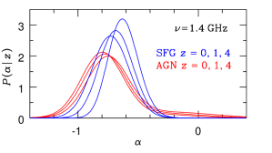
Figure 2: The 1.4 GHz normalized spectral-index distributions $P(\alpha|z)$ of SFGs (blue curves) and AGNs (red curves) for sources at redshifts $z=0,\,1$, and 4 (left to right).

The 1.4 GHz spectral-index distribution of nearby AGNs can by approximated by the the sum of two Gaussians representing the steep-spectrum and flat-spectrum source populations (Condon, 1984):

$$p_{\mathrm{a}}(\alpha|0)=\biggl{(}\frac{A_{\mathrm{steep}}}{\sqrt{2\pi}\sigma_{\mathrm{steep}}}\biggr{)}\exp\biggl{[}-\frac{(\alpha-\bar{\alpha}_{\mathrm{steep}})^{2}}{2\sigma_{\mathrm{steep}}^{2}}\biggr{]}+$$

$$\biggl{(}\frac{A_{\mathrm{flat}}}{\sqrt{2\pi}\sigma_{\mathrm{flat}}}\biggr{)}\exp\biggl{[}-\frac{(\alpha-\bar{\alpha}_{\mathrm{flat}})^{2}}{2\sigma_{\mathrm{flat}}^{2}}\biggr{]}\hskip 11.9501pt$$ (11)

with $A_{\mathrm{steeo}}=0.86$, $\sigma_{\mathrm{steep}}=0.17$, $\bar{\alpha}_{\mathrm{steep}}=-0.8$ and $A_{\mathrm{flat}}=1-A_{\mathrm{steep}}=0.14$, $\sigma_{\mathrm{flat}}=0.38$, $\bar{\alpha}_{\mathrm{flat}}=-0.5$.

The 1.4 GHz spectral-index distribution of nearby SFGs can be represented by a single population, but each SFG has two spectral components—a nonthermal component with a Gaussian spectral-index distribution characterized by mean spectral index $\bar{\alpha}_{\mathrm{n}}\approx-0.8$ and rms width $\sigma_{\mathrm{n}}\approx 0.17$ plus a thermal component with spectral index $\alpha_{\mathrm{t}}\approx-0.1$. At frequency $\nu$ in the source frame, the nonthermal/thermal flux-density ratio $S_{\mathrm{t}}$ is (Condon & Yin, 1990)

$$\frac{S_{\mathrm{n}}}{S_{\mathrm{t}}}\approx 10\biggl{(}\frac{\nu}{\mathrm{GHz}}\biggr{)}^{\alpha_{\mathrm{n}}+0.1}\,.$$ (12)

For $\nu_{0}=1.4\,\mathrm{GHz}$ observations, $S_{\mathrm{n}}/S_{\mathrm{t}}$ declines with redshift in the observed frame from 8 for galaxies at $z=0$ to 2.56 at $z=4$. Because nonthermal emission is always dominant, the mean SFG spectral indices increase only slightly, from $\langle\alpha\rangle\approx-0.72$ at $z=0$ to $\langle\alpha\rangle\approx-0.60$ at $z=4$.

We have assumed that the locally measured spectral-index distributions do not evolve in the source rest frame. Even so, the observed $\nu_{0}=1.4\,\mathrm{GHz}$ spectral-index distributions of sources at redshift $z$ are actually the spectral-index distributions of sources selected at the higher frequency $\nu=(1+z)\nu_{0}$ in the source rest frame and are biased toward “flatter” spectra with higher $\alpha$ (see Condon, 1984, appendix). The expected 1.4 GHz spectral-index distributions of AGNs and SFGs at redshifts $z=0,\,1\,$, and 4 are compared in Figure 2. Small changes in these spectral-index distributions (e.g., varying $\bar{\alpha}_{\mathrm{n}}$ by $\pm 0.1$) actually have very little effect on the predicted source counts and redshift distributions.

4 The Non-evolving Model

We integrated Equation 3 numerically to calculate $S^{2}n(S)$ for the non-evolving model defined by $u_{\mathrm{dex}}(L_{\nu}|z)=u_{\mathrm{dex}}(L_{\nu}|0)$. In order to show the contributions to $S^{2}n(S)$ from sources seen at different lookback times $t_{\mathrm{L}}$, we broke the integration over $z$ into 13 redshift ranges corresponding to the 13 eons of lookback time $0<t_{\mathrm{L}}\mathrm{(Gyr)}<1$, $1<t_{\mathrm{L}}\mathrm{(Gyr)}<2$, $2<t_{\mathrm{L}}\mathrm{(Gyr)}<3$, …, $12<t_{\mathrm{L}}\mathrm{(Gyr)}<13$. These lookback times and redshifts are listed in Table 1.

Table 1: Lookback Times and Redshifts

$t_{\mathrm{L}}$ (Gyr)	Redshift $z$
0	0.000
1	0.076
2	0.160
3	0.256
4	0.366
5	0.494
6	0.648
7	0.835
8	1.075
9	1.395
10	1.855
11	2.602
12	4.111
13	9.977

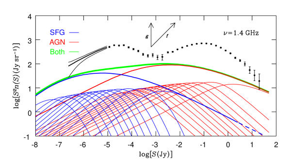
Figure 3: The heavy black curve spanning $-6.6<\log[S\mathrm{(Jy)}]<-5.0$ marks the 1.4 GHz source count $S^{2}n(S)$ determined from the DEEP2 confusion $P(D)$ distribution (Matthews et al., 2021), and the light black curves bound its rms uncertainties. The data points and their rms error bars are the 1.4 GHz DEEP2 direct source counts in the range $-5<\log[S\mathrm{(Jy)}]<-2.7$ Jy and the NVSS counts for $\log[S\mathrm{(Jy)}]>-2.6$. Below the data are curves showing the calculated source counts $S^{2}n(S)$ with no evolution. The thick red curve is the total AGN count, the thick blue curve is the total SFG count, and the wider green curve is their sum, the total non-evolving model source count. The dashed extrapolation of the thick blue curve shows the static Euclidean slope $d[\log[S^{2}n(S)]/d[\log(S)]=-0.5$ expected in the limit of high flux densities where only low-redshift sources exist. The count contributions by sources in the 13 ranges of lookback time are shown by the lighter red and blue curves. From right to left, the lookback time ranges are $t_{\mathrm{L}}=$ 0–1 Gyr, 1–2 Gyr, …, 12–13 Gyr. The arrows labeled $f$ and $g$ indicate how much a light curve covering a limited time range would be shifted by $f=10\times$ luminosity evolution or by $g=10\times$ density evolution in that time range.

With no evolution of the measured local energy-density functions, Equation 3 gives the brightness-weighted source counts $S^{2}n(S)$ plotted in Figure 3. The 13 thin red curves from right to left are the AGN contributions from the 13 eons $0<t_{\mathrm{L}}\mathrm{(Gyr)}<1$ through $12<t_{\mathrm{L}}\mathrm{(Gyr)}<13$, and the thick red curve is the total contribution from all AGNs with $t_{\mathrm{L}}<13\,\mathrm{Gyr}$ ($z<9.977$). The blue curves show the analogous SFG contributions. The wider green curve is their sum, the total source count $S^{2}n(S)$ for the non-evolving model.

At the highest flux densities the model counts indicated by the heavy red, blue, and green curves all must approach the static Euclidean limit of nearby sources $n(S)=kS^{-5/2}$ whose plotted slope is $d\log[S^{2}n(S)]/d\log(S)=-1/2$. The static Euclidean number of sources per steradian stronger than $S$ is $N(>S)=(2k/3)S^{-3/2}$, and the thick curves have been truncated at the flux densities above which they are statistically ill-defined because they imply only one source in the entire sky: $N(>S)=(4\pi)^{-1}$. Non-evolving sources in every $\Delta t_{\mathrm{L}}=1\,\mathrm{Gyr}$ range of lookback time emitted the same total energy, so their contributions to the sky brightness temperature $T_{\mathrm{b}}$ are nearly equal, reduced moderately by the $(1+z)^{\alpha}$ attenuation factor in Equation 9.

Not only does the wide green curve lie well below the observed source count, it is too smooth because the thick red and blue model curves produced by summing over lookback times are much broader than the peaks in the observed brightness-weighted source counts. The arrows labeled $f$ and $g$ in Figure 3 indicate the effects of $10\times$ luminosity or density evolution, respectively, on counts covering a limited time range. Luminosity evolution moves the model curves diagonally upward and to the right while density evolution moves them straight up. The peak in the thick blue curve lies diagonally below and left of the SFG peak in the actual source counts near $\log[S(\mathrm{Jy})]=-4.5$, so nearly pure luminosity evolution should match the observed SFG counts. The peak in the thick red curve must move to the right more than it must move up to match the AGN source-count peak near $\log[S\mathrm{(Jy)]}=-1$, suggesting stronger luminosity evolution and negative density evolution. The strongest evolution should be confined to a narrow range of early times in order to bunch up the light red and blue curves and narrow the peaks of the heavy red and blue curves. Just making the local energy-density functions (Figure 1) match these features of the brightness-weighted source counts (Figure 3) strongly constrains the redshift dependences of the luminosity evolution $f(z)$ and density evolution $g(z)$, without depending on measured redshifts for individual sources.

5 Evolutionary Models

We considered so-called backward evolutionary models ( e.g. a local luminosity function is evolved backwards to match the observed source counts) in which the forms of the AGN and SFG energy-density functions on a log-log plot (Figure 1) do not change, but both populations may evolve independently in both luminosity and density. Pure luminosity evolution $f(z)$ shifts the curves in Figure 1 diagonally upward and to the right, while pure density evolution $g(z)$ shifts them vertically. Then for each source population

$$u_{\mathrm{dex}}(L_{\nu}|z)=g(z)\,u_{\mathrm{dex}}\biggl{[}\frac{L_{\nu}}{f(z)}|0\biggr{]}\,.$$ (13)

For any combination of luminosity evolution $f(z)$ and density evolution $g(z)$, the total comoving spectral power density produced by galaxies of all luminosities at redshift $z$ is proportional to the product $f(z)g(z)$. Thus

$$U_{\mathrm{SFG}}(z)\equiv\int_{-\infty}^{\infty}u_{\mathrm{dex}}(L_{\nu}|z)\,d\log(L_{\nu})=$$

$$f(z)g(z)\int_{-\infty}^{\infty}u_{\mathrm{dex}}(L_{\nu}|0)\,d\log(L_{\nu})~{}.$$ (14)

The total 1.4 GHz spectral luminosity density produced by SFGs today is (Condon et al., 2019)

$$U_{\mathrm{SFG}}(0)=(1.54\pm 0.20)\times 10^{19}\,\mathrm{W\,Hz}^{-1}\,\mathrm{Mpc}^{-3}.$$ (15)

Evolution is often described by functions of the observable source redshift $z$, but for a specific cosmological model (e.g., our $\Lambda$CDM model with $H_{0}=70\,\mathrm{km\,s}^{-1}\mathrm{\,Mpc}^{-1}$ and $\Omega_{\mathrm{m}}=0.3)$, $z$ can be used to calculate the world time $t$ elapsed between the big bang and when the source emitted the radiation we see today. We prefer to describe evolution in terms of $t$ because (1) the evolution experienced by a source depends only on the time $t$ of emission, while $z$ also depends on the time of the observation and (2) $z$ is a very nonlinear measure of time (Table 1), so that equations expressing evolution as a function of $z$ present a distorted picture of the time scales involved. Thus we chose to describe evolution as

$$u_{\mathrm{dex}}(L_{\nu}|t)=g(t)\,u_{\mathrm{dex}}\biggl{[}\frac{L_{\nu}}{f(t)}|0\biggl{]}~{},$$ (16)

subject to the boundary condition ${f(0)\cdot g(0)=0}$ at the big bang and $f(t_{0})=g(t_{0})=1$ at the present time $t_{0}\approx 13.47\mathrm{\,Gyr}$.

Models with strong luminosity evolution predict the existence at high redshifts of extremely luminous AGNs that should have been observed, but were not. Peacock (1985) suggested cutting off the high end of the luminosity function at all redshifts: $\rho(L_{\nu})\propto\exp(-L_{\nu}/L_{\mathrm{c}})$. We applied this exponential cutoff with $L_{\mathrm{c}}=10^{29}\,\mathrm{W\,Hz}^{-1}$.

We model the luminosity and density evolution of both SFGs and AGNs as the product of factors representing their rise at early times and later exponential decay. The rise is modeled in terms of

$$\mathrm{erf}(t)\equiv\frac{2}{\pi^{1/2}}\int_{0}^{t}e^{-x^{2}}dx,$$ (17)

the $S$-shaped error function that increases from $\mathrm{erf}(-\infty)=-1$ through $\mathrm{erf}(0)=0$ to $\mathrm{erf}(+\infty)=+1$, where $t$ is the age of the galaxy in Gyr. An exponential decay at larger $t$ is justified empirically by the UV and IR data points from Madau & Dickinson (2014) that fall on a nearly straight line for $t>4$ Gyr.

We represent luminosity evolution $f(t)$ and density evolution $g(t)$ by the forms:

$$f(t) = \left\{0.5\left[\mathrm{erf}\left(\frac{t-t_{f}}{\tau_{f}}\right)+1\right]\right\}\,\left[\exp\left(\frac{t_{0}-t}{\tau_{1}}\right)\right]$$ (18)

$$g(t) = \left\{0.5\left[\mathrm{erf}\left(\frac{t-t_{g}}{\tau_{g}}\right)+1\right]\right\}\,\left[\exp\left(\frac{t_{0}-t}{\tau_{2}}\right)\right],\qquad$$ (19)

where $t_{f}$ and $t_{g}$ are the midpoint times in Gyr of the turn-on phase of luminosity and density evolution, $\tau_{f}$ and $\tau_{g}$ are the time scales of the turn-on, and $\tau_{1}$ and $\tau_{2}$ are the time scales in Gyr of luminosity and density decay. In Equations 18 and 19 $f$ and $g$ are the products of the turn-on function in curly braces and the decay function in square brackets, and both factors approach unity at $t=t_{0}\approx 13.47\,\mathrm{Gyr}$. The six free parameters are the time scales $\tau_{f}$, $\tau_{g}$, $\tau_{1}$, and $\tau_{2}$ and the midpoint times $t_{f}$ and $t_{g}$. Our choice of functional form has the following desirable features: (1) it is continuous and smoothly varying, (2) the asymptotic rise of the error function to $+1$ at large $t$ makes the rise and decay factors cleanly separable, and (3) the parameters have real physical meanings that can be compared with independent measurements or theories (e.g. the rise time scale $\tau_{\mathrm{r}}$ must agree with theoretical predictions for the minimum time needed for the first galaxies to assemble).

AGNs dominate the 1.4 GHz differential source counts (black points in Figure 4) for all $\log[S\mathrm{(Jy)}]>-3.4$ ($S>0.4\,\mathrm{mJy}$) and SFGs outnumber AGNs at lower flux densities. Nearly all of the AGNs contributing to $S^{2}n(S)$ below $\log[S\mathrm{(Jy)}]\approx-2$ come from the low-luminosity ($L_{\nu}<L^{*}$) end of the AGN energy-density function (Equation 3), which is nearly a power law. Thus all AGN evolutionary models consistent with Equations 13 or 16 and that match $S^{2}n(S)$ for $\log[S\mathrm{(Jy)}]>-2$ must yield similar power-law count contributions throughout the flux-density range dominated by SFGs, as shown by the heavy red line in Figure 4. Consequently, uncertainties in the counts attributed to AGNs have little effect on the modeled SFG counts for $\log[S(\mathrm{Jy})]<-3.4$.

It is mathematically inappropriate to judge the goodness-of-fit of our evolutionary functions through a traditional non-linear least-squares fit (or similar) of the predicted to the observed source counts because the source-counts in adjacent flux-density bins are strongly correlated and thus violate the independence assumption behind these fitting methods. We used Gaussian processes (Rasmussen & Williams, 2006) to accomodate these correlations and derive evolutionary models with appropriately conservative uncertainties in the fitted parameters. There are 6 free parameters in Equations 18 and 19 for both SFGs and AGNs (a total of 12). Because we assumed no late-time density evolution of SFGs, $\tau_{\mathrm{2,SFG}}$ is infinite, so we simultaneously fit only 11 free parements in Equations 18 and 19, plus two more parameters that describe the covariance between data points, using the affine-invariant Monte Carlo Markov Chain (MCMC) code emcee (Foreman-Mackey et al., 2013). We assumed uniform priors for all parameters and enforced a slightly relaxed boundary condition $f(0)\cdot g(0)<0.25\approx 0$. More details of our incorporation of Gaussian processes, the parameter contours resulting from the MCMC fitting, and marginalized posterior distributions can be found in Appendix A.

5.1 AGN radio evolution

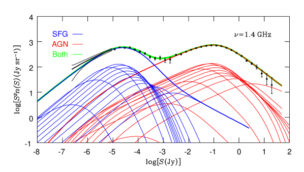
Figure 4: The 1.4 GHz differential source counts between $0.25\,\mu\mathrm{Jy}$ and $25\,\mathrm{Jy}$ are shown with the brightness-weighted normalization $S^{2}n(S)$. The thick black curve spanning $-6.6<\log[S\mathrm{(Jy)}<-5$ is based on the DEEP2 confusion $P(D)$ distribution. The data points with error bars show the 1.4 GHz DEEP2 source counts between in the range $-5<\log[S\mathrm{(Jy)}<-2.6$ Jy and the NVSS counts for $\log[S\mathrm{(Jy)}>-2.6$. The thick curves show the total model counts for AGNs (red), SFGs (blue), and their sum (green). The counts contributed by sources in the 13 ranges of lookback time are shown by the lighter red and blue curves. From right to left, the time ranges are 0–1 Gyr, 1–2 Gyr, …12–13 Gyr.

As expected, pure luminosity evolution ($g=1$) cannot match the observed sharp peak in $S^{2}n(S)$ near $\log[S\mathrm{(Jy)}]=-1$, so we had to supplement luminosity evolution with negative density evolution ($g<1$). Our best model for AGN evolution has:

$$f_{\mathrm{a}}=\left\{0.5\left[\mathrm{erf}\left(\frac{t-3.97}{1.41}\right)+1\right]\right\}\,\left[\exp\left(\frac{t_{0}-t}{2.26}\right)\right]\qquad$$ (20)

and

$$g_{\mathrm{a}}=\left\{0.5\left[\mathrm{erf}\left(\frac{t-2.59}{3.31}\right)+1\right]\right\}\,\left[\exp\left(\frac{t_{0}-t}{-7.62}\right)\right]\qquad$$ (21)

where $t$ is the time in Gyr since the big bang. The negative decay time scale $\tau_{2}=-7.62$ Gyr indicates a slow exponential growth in AGN density at late times. Uncertainties of the derived parameters and their correlations are shown in Appendix A. Figure 5 plots $f_{\mathrm{a}}(t)$ and $g_{\mathrm{a}}(t)$ separately as dotted and dashed red curves, respectively. The total AGN spectral luminosity density

$$U_{\mathrm{AGN}}(t)\equiv\int_{-\infty}^{\infty}u_{\mathrm{dex}}(L_{\nu}|t)\,d\log(L_{\nu})$$ (22)

is proportional to the product $f_{\mathrm{a}}(t)g_{\mathrm{a}}(t)$ shown by the continuous red curve in Figure 5 and $U_{\mathrm{AGN}}(t_{0})=(4.23\pm 0.78)\times 10^{19}\,\mathrm{W\,Hz}^{-1}\,\mathrm{Mpc}^{-3}$ at $\nu=1.4\,\mathrm{GHz}$ (Condon et al., 2019).

Recall from Section 2 and Figure 1 that the local energy-density function of AGNs is well determined down to $\log[L_{\nu}\mathrm{(W\,Hz}^{-1})]\sim 21$, which is four decades below the peak spectral luminosity $\log[L_{\nu}\mathrm{(W\,Hz}^{-1})]\approx 25$. Thus the AGN contribution to the brightness-weighted counts (Figure 4) peaking at $\log[S\mathrm{(Jy)}]\approx-1$ is well determined down to $\log[S\mathrm{(Jy)}]\sim-5$, where the AGN contribution is only $\sim 3$% of the SFG contribution. Any uncertainty in the numbers of fainter AGNs is too small to affect either the total source counts or the counts of SFGs.

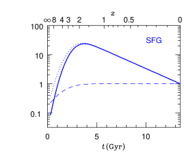
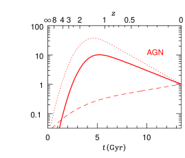
Figure 5: The amounts of radio luminosity evolution $f$ (dotted curves), density evolution $g$ (dashed curves), and their products $fg$ (solid curves) best fitting the observed source counts are shown separately for SFGs (blue) and AGNs (red).

5.2 SFG radio evolution

The radio evolution of SFGs at 1.4 GHz is best fit by

$$f_{\mathrm{s}}=\left\{0.5\left[\mathrm{erf}\left(\frac{t-2.74}{1.30}\right)+1\right]\right\}\left[\exp\left(\frac{t_{0}-t}{2.90}\right)\right]$$ (23)

and

$$g_{\mathrm{s}}=\left\{0.5\left[\mathrm{erf}\left(\frac{t-1.38}{1.99}\right)+1\right]\right\}\,,\quad\quad\qquad~{}$$ (24)

where $t$ is the time in Gyr since the big bang and $\mathrm{erf}(t)$ is the error function. For both luminosity evolution $f_{\mathrm{s}}$ and density evolution $g_{\mathrm{s}}$, the quantities in braces specify the $S$-shaped growth at early times. At later times, the luminosity evolution decays exponentially on a 2.9 Gyr $e$-folding time scale, and there is no density evolution. These evolution functions $f_{\mathrm{s}}$, $g_{\mathrm{s}}$, and their product $f_{\mathrm{s}}g_{\mathrm{s}}$ are shown by the blue curves in Figure 5. Today $U_{\mathrm{SFG}}(t_{0})=(1.54\pm 0.20)\times 10^{19}\,\mathrm{W\,Hz}^{-1}\,\mathrm{Mpc}^{-3}$ (Equation 15), and the resulting fits to the observed faint-source counts are shown by the heavy blue (SFGs only) and green (all sources) curves in Figure 4.

To estimate the overall uncertainty in SFG evolution, we selected those MCMC parameter vectors yielding log-likelihood values in the highest 68% of all samples. In the selected subsample, the minimum amount of SFG evolution consistent with the 1.4 GHz source counts is

$$f_{\mathrm{s}}=\left\{0.5\left[\mathrm{erf}\left(\frac{t-3.10}{1.12}\right)+1\right]\right\}\,\left[\exp\left(\frac{t_{0}-t}{3.04}\right)\right]$$ (25)

$$g_{\mathrm{s}}=\left\{0.5\left[\mathrm{erf}\left(\frac{t-1.79}{0.42}\right)+1\right]\right\}\,\qquad\qquad\quad\quad\quad$$ (26)

and the maximum is

$$f_{\mathrm{s}}=\left\{0.5\left[\mathrm{erf}\left(\frac{t-2.51}{2.50}\right)+1\right]\right\}\,\left[\exp\left(\frac{t_{0}-t}{2.76}\right)\right]$$ (27)

$$g_{\mathrm{s}}=\left\{0.5\left[\mathrm{erf}\left(\frac{t-1.79}{0.97}\right)+1\right]\right\}\,.\qquad\qquad\quad~{}~{}~{}$$ (28)

The broad green curve in Figure 6 shows the range of counts bounded by these minimum and maximum evolution equations. We stress that although the individual parameters describing the luminosity and density evolution have larger uncertainties (Appendix A), the resulting total evolutionary curves remain consistent because the parameters are correlated. This ensures that the resulting implications for the star-formation history of the universe are stable.

When calculating far-ultraviolet (FUV) and FIR luminosity densities of SFGs, Madau & Dickinson (2014) truncated their luminosity functions below $0.03L^{*}_{\mathrm{s}}$ (their equation 14). As a test, we tried truncating our 1.4 GHz SFG luminosity function below $0.03L^{*}_{\mathrm{s}}\approx 6\times 10^{19}\,\mathrm{W\,Hz}^{-1}$. The predicted counts above $S\approx 0.25\,\mu\mathrm{Jy}$ remained well within the green curve in Figure 6 and $\log[S^{2}n(S)]$ fell by only $0.08$ at $S\log[S(\mathrm{Jy})]=-8$.

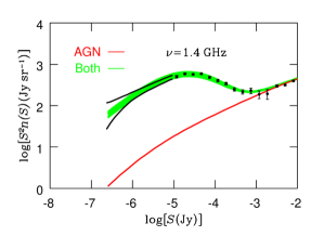
Figure 6: The broad green curve spans the range of total source counts bounded by the minimum and maximum SFG evolution models (Equations 25 through 28). The best-fit AGN counts are shown by the red curve. The black data points with error bars are the DEEP2 and NVSS discrete source counts, and the black curves are the upper and lower limits of the $P(D)$ counts.

5.3 Sky brightness contributed by extragalactic sources at 1.4 GHz

Integrating Equation 5 yields the Rayleigh-Jeans sky brightness temperature contributed by all sources stronger than $S_{0}$:

$$T_{\rm b}(>S_{0})=\left[\frac{\ln(10)c^{2}}{2k_{\rm B}\nu^{2}}\right]\int_{\log S_{0}}^{\infty}S^{2}n(S)d(\log S).$$ (29)

As shown in Figure 7, the model that best fits the brightness-weighted source counts $S^{2}n(S)$ of AGNs adds $T_{\mathrm{b}}\approx 69\,\mathrm{mK}$ to the Rayleigh-Jeans sky brightness temperature at 1.4 GHz, half of which comes from sources stronger than $\log[S\mathrm{(Jy)}]=-1.2$ and 99% from sources with $\log[S\mathrm{(Jy)}]>-4.8$. The acceptable range of SFG model counts adds $T_{\mathrm{b}}=43\pm 6\,\mathrm{mK}$ to the background, of which $\approx 96$% is resolved into sources stronger than $S=0.25\,\mu\mathrm{Jy}$. By integrating the backward evolutionary model for SFG out to increasing redshifts, we determine that half of the total SFG background is produced by sources having redshifts $z<0.93\pm 0.10$.

Figure 7: Model contributions to the 1.4 GHz sky brightness temperature $T_{\mathrm{b}}$ from AGNs (red), SFGs (blue), and the sum of both (green) by sources with flux densities $>S$.

The $\nu=1.4$ GHz sky brightness temperature $T_{\mathrm{b}}$ produced by SFGs (blue curve in Figure 7) was converted to the 1.4 GHz sky brightness $\nu I_{\nu}=2k_{\mathrm{B}}T_{\mathrm{b}}\nu^{3}c^{-2}$ in units of $\mathrm{nW\,m}^{-2}\,\mathrm{sr}^{-1}$ and is shown by the blue curve plotted against the lower abscissa and left ordinate of Figure 8. The $\lambda=160\,\mu\mathrm{m}$ sky brightness of faint FIR sources was measured by Berta et al. (2011) and is shown by the red curve plotted against the upper abscissa and right ordinate of Figure 8. The left end of the red curve at $S_{160\,\mu\mathrm{m}}=0.3\,\mathrm{mJy}$ marks the sensitivity limit of the Herschel PACS $P(D)$ counts, and the right end between $S_{160\,\mu\mathrm{m}}=0.2\,\mathrm{Jy}$ and 1 Jy is the static Euclidean extrapolation (Berta et al., 2011). The upper abscissa was shifted left by the expected mean flux-density ratio $\langle S_{160\,\mu\mathrm{m}}/S_{\mathrm{1.4\,GHz}}\rangle\approx 310$ of faint SFGs at median redshift $\langle z\rangle\approx 1$ (Condon et al., 2019; Berta et al., 2011), and the right ordinate for $\nu I_{\nu}$ was shifted down by $4.16\times 10^{5}$, the flux-density ratio multiplied by the frequency ratio. See Appendix B for the derivation of these numbers. The surprisingly good agreement of the $\lambda=160\,\mu\mathrm{m}$ and $\nu=1.4\,\mathrm{GHz}$ SFG backgrounds is reassuring evidence that (1) contamination of the SFG population by radio-loud AGNs is small and (2) the local FIR/radio correlation does not break down at redshifts $z\sim 1$.

The COBE Far Infrared Absolute Spectrophotometer (FIRAS) measured the total cosmic infrared background contributed by all extragalactic sources to be $\nu I_{\nu}=12.8\pm 6.4\,\mathrm{nW\,m}^{-2}\,\mathrm{sr}^{-1}$ at $\lambda=160\,\mu\mathrm{m}$ (Fixsen et al., 1998), with zodiacal dust emission causing most of the uncertainty. If $\langle S_{160\,\mu\mathrm{m}}/S_{\mathrm{1.4\,GHz}}\rangle\approx 310$, the corresponding 1.4 GHz SFG background $\nu I_{\nu}=3.1\pm 1.5\times 10^{-5}\,\mathrm{nW\,m}^{-2}\,\mathrm{sr}^{-1}$ is consistent with the $\nu I_{\nu}\approx 3.5\pm 0.5\times 10^{-5}\,\mathrm{nW\,m}^{-2}\,\mathrm{sr}^{-1}$ we obtained for SFGs stronger than $S_{\mathrm{1.4\,GHz}}=0.25\,\mu\mathrm{Jy}$. Thus any hypothetical “new population” of fainter radio sources bright enough to produce the large extragalactic brightness at $\nu=3.02\,\mathrm{GHz}$ reported by Fixsen et al. (2011) cannot obey the FIR/radio correlation.

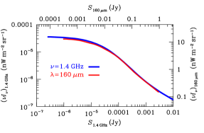
Figure 8: The $\nu=1.4$ GHz sky brightness temperature contributed by SFGs (blue curve in Figure 7) was converted to the cumulative sky brightness $\nu I_{\nu}$ contributed by sources with flux densities $>S_{\mathrm{1.4\,GHz}}$ and is shown by the blue curve (against the lower abscissa and left ordinate). The red curve (against the upper abscissa and right ordinate) shows the $\lambda=160\,\mu$m brightness contributed by sources stronger than $S_{160\,\mu\mathrm{m}}$ (Berta et al., 2011). The curves overlap as shown when $S_{160\,\mu\mathrm{m}}/S_{\mathrm{1.4\,GHz}}=310$ (Appendix B).

6 The Cosmic History of Star Formation

Section 5 describes the radio evolution needed to match the local radio energy-density function to the counts of radio sources associated with SFGs. By themselves, these quantities do not directly constrain the comoving SFRD $\psi(t)$ ($M_{\odot}\,\mathrm{yr}^{-1}\,\mathrm{Mpc}^{-3}$). To calculate the evolving SFRD, we need a prescription relating the radio luminosities of SFGs to their star-formation rates. The radio continuum is an energetically negligible tracer of star formation: the FIR/radio luminosity ratio $\sim 4\times 10^{5}$ of SFGs is comparable with the elephant/mouse mass ratio. Furthermore, most of the 1.4 GHz emission is synchrotron radiation whose luminosity depends on poorly known quantities such as the interstellar magnetic field strength and ambient radiation energy density. It took the discovery of the surprisingly strong empirical FIR/radio correlation in nearby galaxies (Helou et al., 1985) to convert radio continuum photometry of SFGs from a hobby into a quantitative science.

6.1 The linear FIR/radio correlation

If the FIR/radio correlation is linear ($L_{\mathrm{FIR}}\propto L_{\mathrm{1.4\,GHz}})$ and does not evolve, then only the local FIR/radio flux-density ratio is needed to convert from radio luminosity to star-formation rate. That ratio is usually expressed in terms of the dimensionless constant $q$ (Helou et al., 1985):

$$q\equiv\log\biggl{[}\frac{\mathrm{FIR}/(3.75\times 10^{12}\,\mathrm{Hz})}{S\mathrm{(1.4\,GHz)}}\biggr{]}~{},$$ (30)

where FIR is the flux between 42.5 and $122.5\,\mu$m in units of W m^-2 estimated from the IRAS 60 and $100\,\mu$m flux densities in Jy

$$\mathrm{FIR}=1.26\times 10^{-14}[2.58S(60\,\mu\mathrm{m})+S(100\,\mu\mathrm{m})]\,$$ (31)

and $3.75\times 10^{12}\,\mathrm{Hz}$ is the frequency corresponding to the midpoint wavelength $\lambda=80\,\mu\mathrm{m}$. (Beware that the FIR in Equation 31 is a flux with units of W m^-2 so the numerator in Equation 30 is a flux density with units of $\mathrm{W\,m}^{-2}\,\mathrm{Hz}^{-1}$. Thus either the denominator $S\mathrm{(}1.4\,\mathrm{GHz})$ should be specified in units of $\mathrm{W\,m}^{-2}\,\mathrm{Hz}^{-1}=10^{26}\,\mathrm{Jy}$ or, if $S\mathrm{(}1.4\,\mathrm{GHz})$ is specified in Jy, the numerator should be multiplied by $10^{26}$.) For the flux-limited IRAS sample of galaxies with $S(60\,\mu\mathrm{m})>2\,\mathrm{Jy}$, Yun et al. (2001) reported a nearly linear FIR/radio correlation with scatter $\sigma=0.26$ in the $q$ values of individual galaxies and sample mean $\langle q\rangle=2.34\pm 0.01$.

If the 1.4 GHz spectral luminosities of SFGs are indeed proportional to their star formation rates and the constant of proportionality does not evolve, then the radio evolution of SFGs implies SFRD evolution

$$\frac{\psi(t)}{\psi_{0}}=f_{\mathrm{s}}(t)g_{\mathrm{s}}(t)\,,$$ (32)

where $\psi_{0}\equiv\psi(t_{0})$ is the SFRD now. The thick blue curve in Figure 9 indicates the radio SFRD evolution based on Equations 23 and 32.

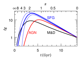
Figure 9: The thick blue curve, which is the same as the thick blue curve in Figure 5, shows the best-fit evolution of the radio SFRD if $\psi/\psi_{0}=f_{\mathrm{s}}g_{\mathrm{s}}$ for SFGs, and the thin blue curves indicate the minimum and maximum amounts of evolution specified by Equations 25 through 28. All are significantly higher than the black curve showing the evolution $\psi/\psi_{0}=fg$ of the SFRD based on FUV and FIR data (Madau & Dickinson, 2014, equation 15). The red curve is our best fit to the product $f_{\mathrm{a}}g_{\mathrm{a}}$ for AGN. It is closer to the Madau & Dickinson (2014) curve for stars, indicating comparable amounts of SFG and AGN evolution, but the AGN peak lags by $\gtrsim 1\,\mathrm{Gyr}$. Abscissa: time $t$ in Gyr since the big bang. Ordinate: Normalized evolution $fg$.

Using FIR and FUV data, Madau & Dickinson (2014) estimated the evolving SFRD and approximated it by the function

$$\frac{\psi(z)}{\psi_{0}}\approx\frac{(1+z)^{2.7}}{1+[(1+z)/2.9]^{5.6}}$$ (33)

shown by the black curve in Figure 9. Both the blue and black curves peak around the same “cosmic noon” near $t=3\,\mathrm{Gyr}$, $z=2$ and decline exponentially at later times, but the radio estimate implies a significantly stronger overall evolution of the SFRD. If the FIR/radio correlation is linear and the 1.4 GHz energy density function underwent luminosity evolution specified by Equation 33, the predicted radio source counts of SFGs would fall well below the observed counts. Integrating the predicted radio source counts (see Equation 29) determines that SFGs would contribute only $T_{\mathrm{b}}=21\,\mathrm{mK}$ to the sky brightness temperature.

About half of the observed $43\,\mathrm{mK}$ SFG background is produced by sources with $\log[S\mathrm{(Jy)}]>-4.8$ ($S>16\,\mu\mathrm{Jy}$), nearly half by sources with $-6.6<\log[S\mathrm{(mJy)}]<-4.8$, and only $\sim 4$% of the model SFG background is produced by sources below our $P(D)$ count limit $\log[S\mathrm{(Jy)]}=-6.6$ ($S=0.25\,\mu\mathrm{Jy}$). Stronger luminosity evolution and negative density evolution with fixed $f_{\mathrm{s}}(z)g_{\mathrm{s}}(z)$ could fit the 1.4 GHz source counts above $\log[S\mathrm{(Jy)}]\sim-4.8$, but no separate adjustments of luminosity evolution $f$ or density evolution $g$ consistent with a given $\psi/\psi_{0}$ or product $fg$ can significantly change these SFG contributions to $T_{\mathrm{b}}$ and match the counts between $\log[S\mathrm{(Jy)]}=-6.6$ and $\log[S\mathrm{(Jy)]}=-4.8$. We conclude that the large difference between the radio and FUV/FIR SFRDs cannot be avoided if the FIR/radio correlation is linear and does not evolve. Thus authors who assume a linear FIR/radio correlation to model deep FIR and radio counts necessarily find that $q$ decreases with redshift; e.g., Delhaize et al. (2017) used sensitive Jansky Very Large Array (VLA) and Herschel images to find $q\propto(1+z)^{-0.19\pm 0.01}$ in the redshift range $0<z<6$.

6.2 The nonlinear FIR/radio correlation

The difference between SFRD evolution estimates based on our 1.4 GHz data and on the FUV/FIR data in Madau & Dickinson (2014) can be reduced if the FIR/radio correlation is sub-linear; that is, $x<1$ in $L_{\mathrm{FIR}}\propto L_{\mathrm{1.4\,GHz}}^{x}$. To determine the degree of nonlinearity, we measured the local $q$ (Equation 30) as a function of $\log[L\mathrm{(1.4\,GHz)}]$. The $q$ distribution of sources in a flux-limited sample is biased by the selection frequency; thus the mean $\langle q\rangle$ in a FIR-selected sample is higher than $\langle q\rangle$ in a radio-selected sample (see Condon, 1984, appendix). Such biases can be removed by assigning to each source a weight inversely proportional to the maximum volume $V_{\mathrm{max}}$ in which it could remain in the sample, yielding the unbiased volume-limited distribution of $q$.

To measure the unbiased local distribution of $q$, we started with the large sample of NVSS sources stronger than $S=2.5\,\mathrm{mJy}$ used in Section 2 to determine the local radio luminosity function, but kept only the sources with $S\geq 5\,\mathrm{mJy}$ to ensure that nearly all (98%) of the sample SFGs were detected by IRAS and have accurately measured values of $q$. Although purely flux-limited samples of all radio sources with $S\geq 5\,\mathrm{mJy}$ are dominated by faint and distant ($\langle z\rangle\sim 1$) AGNs, our bright ($k_{20fe}<+11.75$) and thus local ($\langle z\rangle\sim 0.02$) sample is not, so the SFGs can be separated from the AGNs, as shown in Figure 1.

This sample was divided into 1.4 GHz luminosity bins of width $\Delta\log(L_{\nu})=0.2$ centered on $\log(L_{\nu})=19.7$ through $23.5$. We weighted the value of $q$ for each source by its $L_{\nu}/V_{\mathrm{max}}$ ratio, where $V_{\mathrm{max}}$ is the smaller of its $\lambda=2.16\,\mu\mathrm{m}$ or $\nu=1.4\,\mathrm{GHz}$ maximum volumes, so that the overall weighted mean of the entire sample is an unbiased measure of the volume-limited FIR/radio luminosity density ratio. Within each narrow radio luminosity bin, the rms scatter of individual $q$ values is only $\sigma_{q}\approx 0.16$. The weighted means $\langle q\rangle$ and their rms uncertainties $\sigma_{\langle q\rangle}$ are plotted for all populated luminosity bins in Figure 10. The bent line in Figure 10 shows the fit

$$\langle q\rangle= 2.69-0.147[\log(L_{\nu})-19.1] ~{}~{}\mathrm{if}~{}\log(L_{\nu})<22.5\quad$$

$$\langle q\rangle= 2.19~{}~{}\mathrm{if}~{}\log(L_{\nu})\geq 22.5\qquad$$ (34)

indicating a clearly sub-linear FIR/radio relation $L_{\mathrm{FIR}}\propto L_{\nu}^{0.85}$ in the 1.4 GHz luminosity range $\log(L_{\nu})<22.5$ that includes $>90$% of nearby SFGs. Sub-linearity implies that FIR luminosity evolution, and hence SFRD evolution, is not as strong as 1.4 GHz evolution. The volume-limited average for nearby SFGs of all luminosities is $\bar{q}=2.30\pm 0.01$. These results are quite stable, varying by $\sim 0.1$% when the 2% of galaxies with only IRAS upper limits are included or excluded. To the extent that the star-formation rates of galaxies are proportional to their stellar masses $M_{\star}$ (Brinchmann et al., 2004) (that is, there is a “main sequence” of star-forming galaxies), the recent finding that $dq/d\log(M_{\star})=-0.148\pm 0.013$ nearly independent of redshift (Delvecchio et al., 2020) is consistent with our sublinear local FIR/radio correlation $dq/d\log(L_{\nu})=-0.147$ and our assumption that the FIR/radio correlation itself does not evolve with redshift. While we know that the local FIR/radio correlation is sublinear and can fit our data with a non-evolving FIR/radio correlation, we cannot demonstrate that no such evolution exists.

Figure 10: The logarithmic FIR/radio ratio parameter decreases as $d\langle q\rangle/d\log(L_{\nu})=-0.147$ below $\log[L_{\nu}(\mathrm{W\,Hz}^{-1})]=22.5$ and is a constant $\langle q\rangle=2.19$ at higher luminosities.

For our evolutionary models, the FIR luminosities $L_{\mathrm{FIR}}$ of individual SFGs at any redshift were estimated by inserting $\langle q\rangle$ values from Equation 6.2 into

$$L_{\mathrm{FIR}}=3.75\times 10^{12}\,\mathrm{Hz}\cdot L_{\mathrm{1.4\,GHz}}\cdot 10^{\langle q\rangle}~{}.$$ (35)

The matching energy-density equation is

$$\biggl{[}\frac{u_{\mathrm{dex}}(\mathrm{FIR})}{\mathrm{W\,Mpc}^{-3}}\biggr{]}=3.75\times 10^{12}\,\mathrm{Hz}\cdot\biggl{[}\frac{u_{\mathrm{dex}}(\mathrm{1.4\,GHz})}{\mathrm{W\,Hz}^{-1}\,\mathrm{Mpc}^{-3}}\biggr{]}\cdot 10^{q}~{}.$$ (36)

6.3 Converting $L_{\mathrm{FIR}}$ to star-formation rates

The total SFR associated with a given infrared luminosity depends on the assumed initial mass function (IMF) and stellar model spectra. Murphy et al. (2011) assumed a Kroupa (2001) IMF and used the Starburst99 spectrum integrated over the infrared (IR) band covering $8<\lambda(\mu\mathrm{m})<1000$ to obtain

$$\biggl{(}\frac{\mathrm{SFR}}{M_{\odot}\,\mathrm{yr}^{-1}}\biggr{)}=3.88\times 10^{-37}\biggl{(}\frac{L_{\mathrm{IR}}}{\mathrm{W}}\biggr{)}~{}.$$ (37)

The widely referenced conversion factor in table 1 of Kennicutt & Evans (2012) is based on this Murphy et al. (2011) value. A Salpeter IMF Salpeter (1955) has a larger fraction of low-mass stars and implies that total SFRs including all stars in the mass range $0.1<M_{\odot}<100$ are factor of $1/0.66=1.52$ higher for a given $L_{\mathrm{IR}}$. Most nearby SFGs have only measured FIR luminosities, not IR luminosities. Bell (2003) compared the $q$ values for IR and FIR luminosities and found $\langle L_{\mathrm{IR}}/L_{\mathrm{FIR}}\rangle\approx\mathrm{dex}(2.64-2.36)\approx 1.91$, so for a Kroupa (2001) IMF

$$\biggl{(}\frac{\mathrm{SFR}}{M_{\odot}\,\mathrm{yr}^{-1}}\biggr{)}=7.39\times 10^{-37}\biggl{(}\frac{L_{\mathrm{FIR}}}{\mathrm{W}}\biggr{)}~{}.$$ (38)

Combining these results and integrating over $\log L_{\nu}$ yields our radio estimate of the evolving SFRD $\psi$ for a Kroupa (2001) IMF at any time $t$ :

$$\biggl{[}\frac{\psi(t)}{M_{\odot}\,\mathrm{yr}^{-1}\,\mathrm{Mpc}^{-3}}\biggr{]}=7.39\times 10^{-37}\,\cdot\,3.75\times 10^{12}\mathrm{\,Hz}\,\cdot$$

$$\int\biggl{[}\frac{u_{\mathrm{dex}}(L_{\nu}|t)\cdot 10^{\langle q(L_{\nu})\rangle}}{\mathrm{W\,Hz}^{-1}\,\mathrm{Mpc}^{-3}}\biggr{]}d\log(L_{\nu})\,,\qquad$$ (39)

where $L_{\nu}$ is the 1.4 GHz spectral luminosity. Again, for a Salpeter (1955) IMF, $\psi$ is a factor of 1.52 larger. For a Salpeter (1955) IMF and $U_{\mathrm{SFG}}=1.54\pm 0.2\times 10^{19}\mathrm{\,W\,Hz}^{-1}\,\mathrm{Mpc}^{-3}$ (Equation 15), $\psi(t_{0})=0.0128\,M_{\odot}\,\mathrm{yr}^{-1}\,\mathrm{Mpc}^{-3}$ is the radio estimate of the SFRD today.

Figure 11 compares our 1.4 GHz estimate of the evolving SFRD $\psi(t)$ (thick blue curve) with the standard Madau & Dickinson (2014) FUV/FIR data points and estimate (black curve), all for a Salpeter (1955) IMF. Our best 1.4 GHz estimate is well approximated by

$$\log\biggl{[}\frac{\psi(t)}{M_{\odot}\,\mathrm{yr}^{-1}\,\mathrm{Mpc}^{-3}}\biggr{]}=-3.473+1.818\biggl{(}\frac{t}{\mathrm{Gyr}}\biggr{)}\quad\quad$$

$$-3.653\biggl{(}\frac{t}{\mathrm{Gyr}}\biggr{)}^{2}+0.02216\biggl{(}\frac{t}{\mathrm{Gyr}}\biggr{)}^{3}\qquad\qquad$$ (40)

when $0.5<t\mathrm{(Gyr})<5$ and by

$$\log\biggl{[}\frac{\psi(t)}{M_{\odot}\,\mathrm{yr}^{-1}\,\mathrm{Mpc}^{-3}}\biggr{]}=-0.0529-0.1373\biggl{(}\frac{t}{\mathrm{Gyr}}\biggr{)}$$ (41)

when $t\mathrm{(Gyr)}>5$. The light blue curves indicate the range of SFRDs consistent with the $13\%$ uncertainty in the SFRD today quadratically added to the SFRD ranges from our acceptable evolutionary models (Section 5.2). To convert Figure 11 from a Salpeter (1955) IMF to a Kroupa (2001) IMF, subtract $0.18$ from $\log(\psi)$. The sub-linear FIR/radio correlation has increased the 1.4 GHz late-time $e$-folding time scale $\tau=2.9^{+0.07}_{-0.07}\,\mathrm{Gyr}$ (Equation 23) to $\tau=3.2^{+0.08}_{-0.08}\,\mathrm{Gyr}$ for the SFRD $\psi$, bringing it closer to but still smaller than the Madau & Dickinson (2014) $\tau\approx 4.4\,\mathrm{Gyr}$.

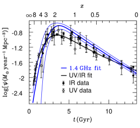
Figure 11: The evolving SFRD $\psi$ for a Salpeter (1955) IMF is shown as a function of time $t$ (Gyr) since the big bang. The UV and IR data points and the black curve fitted to Equation 33 with $\psi_{0}=0.015\,M_{\odot}\,\mathrm{yr}^{-1}\,\mathrm{Mpc}^{-3}$ are from the Madau & Dickinson (2014) review. The heavy blue curve is our best-fit 1.4 GHz SFRD estimate, and the light blue curves bound the range of acceptable fits to our 1.4 GHz data.

7 Discussion and Conclusions

This paper presents an independent estimate of the cosmic star-formation history based on radio evolutionary models matching the 1.4 GHz local luminosity function and counts of sources as faint as $S=0.25\,\mu\mathrm{Jy}$ at 1.4 GHz, the flux density of the Milky Way at $z=4$ with $10\times$ luminosity evolution.

• Radio source evolution of AGNs and SFGs at 1.4 GHz was determined by matching local luminosity functions $\rho_{\mathrm{dex}}(L_{\nu})$ or local energy-density functions $u_{\mathrm{dex}}(L_{\nu})$ with the brightness-weighted source counts $S^{2}n(S)$.

• We made the first measurement of the local volume-limited FIR/radio correlation and found it to be sub-linear: $L_{\mathrm{FIR}}\propto L_{\mathrm{1.4\,GHz}}^{0.85}$.

• We used our sub-linear FIR/radio correlation to convert radio-source evolution to an evolving SFRD $\psi$ ($M_{\odot}\,\mathrm{yr}^{-1}\,\mathrm{Mpc}^{-3}$). This radio estimate reproduces the usual SFRD peak near $z\approx 2$, but the peak SFRD indicates stronger evolution than the standard FUV/FIR estimate (Madau & Dickinson, 2014).

7.1 What are the main strengths and weaknesses of this radio SFRD model?

• The 1.4 GHz emission from a star-forming galaxy is a mixture of synchrotron radiation from electrons accelerated in core-collapse supernova remnants of $M>8M_{\odot}$ stars and thermal bremsstrahlung from Hii regions, making it less sensitive than FIR luminosity to contamination by older stellar populations. However, radio emission is more vulnerable to unrecognized AGN contamination, primarily in galaxies with high SFRs and high radio luminosities. The sample of SFGs used to generate the local 1.4 GHz luminosity function was carefully vetted (Condon et al., 2019), and the local radio SFRD $\psi(t_{0})=0.0128\,M_{\odot}\,\mathrm{yr}^{-1}\,\mathrm{Mpc}^{-3}$ is slightly lower than the FUV/FIR $\psi(t_{0})=0.015\,M_{\odot}\,\mathrm{yr}^{-1}\,\mathrm{Mpc}^{-3}$ (both for a Salpeter (1955) IMF). Thus the local 1.4 GHz sample does not seem to be badly contaminated. AGN contamination of SFGs at high redshifts might cause their source counts and hence radio evolution to be overestimated, but the excellent agreement of the background brightnesses $\nu I_{\nu}$ produced by SFGs at $\nu=1.4\,$GHz and $\lambda=160\,\mu\mathrm{m}$ (Figure 8) is reassuring.

• AGNs dominate the source counts above $S\approx 0.4\,\mathrm{mJy}$, but their contributions to the total counts of significantly fainter sources can be estimated accurately because they are smooth power laws at the low-luminosity end of their energy density function.

• The peak contribution of SFGs to $S^{2}n(S)$ occurs near $S=10\,\mu\mathrm{Jy}$, and about half the total SFG contribution is from fainter sources. The main obstacle to radio measurements of the SFRD has been measuring accurate source counts down to $S\approx 0.25\,\mu\mathrm{Jy}$. That is now possible, but only statistically via the confusion $P(D)$ distribution (Matthews et al., 2021), so it is not possible to identify individual $S\approx 0.25\,\mu\mathrm{Jy}$ sources or measure their redshifts. Instead, the amounts of luminosity evolution $f$ and density evolution $g$ depend entirely on fitting features in the local energy-density functions to features in the brightness-weighted source counts. Only smoothly varying $f$ and $g$ can be modeled accurately, and rare populations (e.g., SFGs at very high redshifts) can easily be overlooked. The 1.4 GHz spectra of SFGs are power laws with spectral indices near $\alpha=-0.7$, so their K-corrections are easy to calculate but large enough that 1.4 GHz SFRDs are best determined at redshifts up to and slightly beyond “cosmic noon,” but submm continuum sources with low or negative K-corrections and submm spectral lines are better for detecting SFGs at redshifts $z\gtrsim 4$.

• The dominant synchrotron luminosity at 1.4 GHz is only an energetically negligible tracer of star formation and is not simply proportional to the SFR; it depends on unknown or unrelated quantities such as the interstellar magnetic field strength and inverse-Compton (IC) scattering off the ambient radiation field produced by starlight plus the cosmic microwave background (CMB). Thus the use of 1.4 GHz luminosity to measure the SFR is justified primarily by the empirical FIR/radio correlation. The locally measured FIR/radio correlation might fail at high redshifts owing to IC scattering losses off the CMB $\propto(1+z)^{4}$. This does not seem to be a problem because it can only lower the radio SFRD estimate, and the radio SFRD estimate is slightly higher than expected. The FIR/radio correlation is often treated as being linear, but we found it to be sub-linear: $L_{\mathrm{FIR}}\propto L_{\mathrm{1.4\,GHz}}^{0.85}$. Sub-linearity significantly reduces the discrepancy between the radio and FIR SFRD models as shown by Figures 9 and 11, so the resulting radio SFRD models lie above but just within the error bars of the FIR data points.

Appendix A Gaussian Process Model Fitting

Radio source counts and their uncertainties in individual flux-density bins are not independent from their neighbors, so fitting models to these data by minimizing $\chi^{2}$ will underestimate the model uncertainties and may introduce biases. We use Gaussian processes to allow for possible correlations and derive evolutionary models with conservative uncertainties in the parameters.

For a complete review of the theory behind (and applications of) Gaussian processes, we refer the reader to Rasmussen & Williams (2006). Briefly, a Gaussian process is a generalization of a Gaussian probability distribution that takes into account stochastic effects like correlated noise by modeling both your the function (the physical model) and also the covariance function. This ability presents itself through the generalization of the likelihood function as a matrix equation

$$\log p(\{y_{n}\}\,|\,\{{\boldsymbol{x}}_{n},\,\sigma_{n}\},\,{\boldsymbol{\theta}}) = -\frac{1}{2}\,{{\boldsymbol{r}}_{\boldsymbol{\theta}}}^{\mathrm{T}}\,K^{-1}\,{{\boldsymbol{r}}_{\boldsymbol{\theta}}}-\frac{1}{2}\,\log\det K-\frac{N}{2}\,\log(2\,\pi)$$ (A1)

where ${\boldsymbol{r}}_{\boldsymbol{\theta}}$ is the residual vector

$${{\boldsymbol{r}}_{\boldsymbol{\theta}}}^{\mathrm{T}}=\left(\begin{array}[]{ccc}y_{1}-f({\boldsymbol{x}}_{1};\,{\boldsymbol{\theta}})&\cdots&y_{N}-f({\boldsymbol{x}}_{N};\,{\boldsymbol{\theta}})\end{array}\right)$$ (A3)

and $K$ is the “covariance matrix.” When the data points are independent, the off-diagonal elements of the $N\times N$ matrix $K$ are 0. Covariance between data points $n$ and $m$ are quantified by non- zero $n,\,m$ off-diagonal elements. In our case (and in most others) it is difficult or impossible to estimate the covariances accurately, which makes the ability to fit for them using Gaussian processes especially helpful.

It would be extremely computationally expensive to add $\sim N^{2}$ parameters that need to be fit. Instead of fitting each $n,\,m$-th element of the matrix directly, we parameterize it using a functional form

$$K_{n,\,m} = {\sigma_{n}}^{2}\,\delta_{n,\,m}+k({\boldsymbol{x}}_{n},\,{\boldsymbol{x}}_{m};\,{\boldsymbol{\alpha}})$$ (A4)

where $\delta_{n,\,m}$ is the Kronecker delta and $k({\boldsymbol{x}}_{n},\,{\boldsymbol{x}}_{m};\,{\boldsymbol{\alpha}})$ is the covariance function (or kernel) that parameterizes by ${\boldsymbol{\alpha}})$ the covariance between by data points using a functional form. It is then up to the user to choose a covariance function that approximates the (unknown) actual covariance between data points.

Using the python Gaussian process package george (Ambikasaran et al., 2015), we first maximized the log-likelihood for various covariance functions to determine which was best suited for our data. We know that the covariance between data points varies smoothly, and found that the “squared exponential covariance function” maximizes the log-likelihood

$$k_{\mathrm{SE}}(r)=\sigma_{f}^{2}\exp\left(-\frac{r^{2}}{2l^{2}}\right),$$ (A5)

where $r=|{\boldsymbol{x}}_{n}-{\boldsymbol{x}}_{m}|$ defines the distance between data points, $\sigma_{r}^{2}$ is a positive constant describing the process variance, and $l$ defines the characteristic length scale (the reach of influence on neighboring data points).

We used the generalized likelihood function (Equation A1) with the squared exponential covariance function and the affine-invariant Markov Chain Monte Carlo code emcee (Foreman-Mackey et al., 2013) to fit for the 13 free parameters: 5 in the equations governing the evolution of SFGs: $t_{\mathrm{f,SFG}},\,\tau_{\mathrm{f,SFG}},\,\tau_{\mathrm{SFG}},\,t_{\mathrm{g,SFG}}$, and $\tau_{\mathrm{g,SFG}}$, 6 in the evolutionary equations for AGNs: $t_{\mathrm{f,AGN}}$, $\tau_{\mathrm{f,AGN}}$, $\tau_{\mathrm{1,AGN}}$, $t_{\mathrm{g,AGN}}$, $\tau_{\mathrm{g,AGN}}$, and $\tau_{\mathrm{2,AGN}}$, plus the two parameters of the covariance function: $\sigma_{f}^{2}$ and $l$. We assumed uniform priors for the input parameters and enforce the boundary condition $f(0)\cdot g(0)\approx 0$. The resulting SFG evolutionary parameter contours and marginalized posterior distributions are shown in Figure 12. The parameter values derived from their marginalized posterior distributions and their 1$\sigma$ uncertainties are listed in Table 2. Source counts resulting from 15 randomly-selected parameter samples from these posterior distributions and the corresponding evolutionary functions are shown in Figure 13.

Table 2: MCMC-derived parameter values and uncertainties

Parameter	Best-fit value	$+1\sigma$	$-1\sigma$
t_f,SFG	2.74	+0.32	-0.26
τ_f,SFG	1.30	+0.18	-0.29
τ_1,SFG	2.90	+0.07	-0.07
t_g,SFG	1.38	+0.29	-0.44
τ_g,SFG	1.99	+0.67	-0.76
t_f,AGN	3.97	+0.36	-0.51
τ_f,AGN	1.41	+0.54	-0.65
τ_1,AGN	2.26	+0.05	-0.05
t_g,AGN	2.59	+0.75	-0.89
τ_g,AGN	3.31	+1.09	-0.81
τ_2,AGN	$-$7.62	+0.84	-0.67

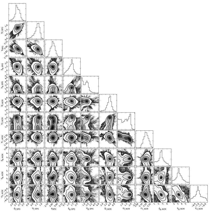
Figure 12: Parameter contours and marginalized posterior distributions from the MCMC chains.

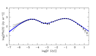
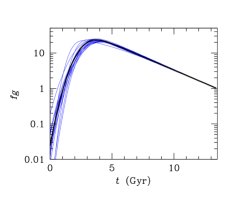
Figure 13: Left: 1.4 GHz brightness-weighted source count data shown as black points (source counts derived via $P(D)$ confusion analysis shown as black curves). Fifteen randomly selected parameter vectors from the MCMC fitting routine were used to generate predicted source counts (blue curves). Right: The corresponding fifteen total evolutionary ($fg$) functions for SFGs. The best-fitting total evolutionary function is shown as the black solid line.

Appendix B The median IR/radio flux-density ratio of faint SFGs

The median redshift of faint SFGs selected at either $\nu=1.4$ GHz (Section 5.3) or $\lambda=160\,\mu$m (Berta et al., 2011) is $\langle z\rangle\approx 1$, so the observed flux-density ratio $\langle S_{160\,\mu\mathrm{m}}/S_{\mathrm{1.4\,GHz}}\rangle$ equals $\langle S_{80\,\mu\mathrm{m}}/S_{\mathrm{2.8\,GHz}}\rangle$ in the source rest frame. We estimated the latter ratio in terms of the locally measured quantities FIR (Equation 31) and $q$ (Equation 30).

Nearby SFGs have $\langle q\rangle\approx 2.30$ (Section 6.2) for flux densities measured at 1.4 GHz and SFGs have radio spectral indices $\langle\alpha\rangle\approx-0.7$ (Section 3), so $\langle q\rangle\approx 2.51$ for flux densities measured at 2.8 GHz in the source rest frame. Local SFGs typically have FIR flux-density ratios $\langle S_{100\,\mu\mathrm{m}}/S_{60\,\mu\mathrm{m}}\rangle\sim 2$ (Condon et al., 2019), so linear interpolation in $\log(S),\,\log(\nu)$ between $S_{60\,\mu\mathrm{m}}\approx 0.68\,\mathrm{Jy}$ and $S_{100\,\mu\mathrm{m}}=2S_{60\,\mu\mathrm{m}}$ yields $S_{80\,\mu\mathrm{m}}=1\,\mathrm{Jy}$ and $\mathrm{FIR}=3.91\times 10^{-14}\,\mathrm{W\,m}^{-2}$. This result is nearly independent of the ratio $S_{100\,\mu\mathrm{m}}/S_{60\,\mu\mathrm{m}}$; even for relatively warm SFGs with $S_{100\,\mu\mathrm{m}}/S_{60\,\mu\mathrm{m}}\sim 1$, the value of FIR corresponding to $S_{\mathrm{80\,\mu\mathrm{m}}}=1\,\mathrm{Jy}$ changes by $<10$%. Solving Equation 30 for $S_{2.8\,\mathrm{GHz}}$ when $S_{80\,\mu\mathrm{m}}=1\,\mathrm{Jy}$ gives

$$\frac{S_{160\,\mu\mathrm{m}}}{S_{1.4\,\mathrm{GHz}}}=\frac{S_{80\,\mu\mathrm{m}}}{S_{2.8\,\mathrm{GHz}}}=\frac{10^{2.51}\cdot 3.75\times 10^{12}\,\mathrm{Hz}}{3.91\times 10^{-14}\,\mathrm{W\,m}^{-2}\cdot 10^{26}\,\mathrm{Jy\,W}^{-1}\,\mathrm{m}^{2}\,\mathrm{Hz}}\approx 310\,.$$ (B1)

This flux-density ratio was used to shift the $S_{\nu}$ and $\nu I_{\nu}$ axes of Figure 8 and demonstrate the excellent agreement between the observed $\lambda=160\,\mu\mathrm{m}$ and $\nu=1.4\,\mathrm{GHz}$ backgrounds produced by SFGs.

A small change in $\langle z\rangle$ has only a small effect on the calculated ratio $S_{160\,\mu\mathrm{m}}/S_{1.4\,\mathrm{GHz}}$:

$$\Bigg{|}d\log\biggl{(}\frac{S_{160\,\mu\mathrm{m}}}{S_{1.4\,\mathrm{GHz}}}\biggr{)}\Bigg{|}<\big{|}(\alpha_{\mathrm{FIR}}-\alpha)d\log(1+\langle z\rangle)\big{|}~{}.$$ (B2)

For any $1<S_{100\,\mu\mathrm{m}}/S_{60\,\mu\mathrm{m}}<2$ and $0.8<\langle z\rangle<1.2$, $\log(S_{160\,\mu\mathrm{m}}/S_{1.4\,\mathrm{GHz}})$ varies by less than $\pm 0.03$.

References

- Ambikasaran et al. (2015) Ambikasaran, S., Foreman-Mackey, D., Greengard, L., Hogg, D. W., & O’Neil, M. 2015, IEEE Transactions on Pattern Analysis and Machine Intelligence, 38, 252
- Bell (2003) Bell, E. F. 2003, ApJ, 586, 794
- Bendo et al. (2010) Bendo, G. J., Wilson, C. D., Pohlen, M., et al. 2010, A&A, 518, L65
- Berkhuijsen (1984) Berkhuijsen, E. M. 1984, A&A, 140, 431
- Berta et al. (2011) Berta, S., Magnelli, B., Nordon, R., et al. 2011, A&A, 532, A49
- Brinchmann et al. (2004) Brinchmann, J., Charlot, S., White, S. D. M., et al. 2004, MNRAS, 351, 1151
- Chabrier (2003) Chabrier, G. 2003, PASP, 115, 763
- Coe et al. (2013) Coe, D., Zitrin, A., Carrasco, M., et al. 2013, ApJ, 762, 32
- Condon (1984) Condon, J. J. 1984, ApJ, 287, 461
- Condon (1992) —. 1992, ARA&A, 30, 575
- Condon et al. (1998) Condon, J. J., Cotton, W. D., Greisen, E. W., et al. 1998, AJ, 115, 1693
- Condon & Matthews (2018) Condon, J. J., & Matthews, A. M. 2018, PASP, 130, 073001
- Condon et al. (2019) Condon, J. J., Matthews, A. M., & Broderick, J. J. 2019, ApJ, 872, 148
- Condon & Yin (1990) Condon, J. J., & Yin, Q. F. 1990, ApJ, 357, 97
- Condon et al. (2012) Condon, J. J., Cotton, W. D., Fomalont, E. B., et al. 2012, ApJ, 758, 23
- Delhaize et al. (2017) Delhaize, J., Smolčić, V., Delvecchio, I., et al. 2017, A&A, 602, A4
- Delvecchio et al. (2020) Delvecchio, I., Daddi, E., Sargent, M. T., et al. 2020, arXiv e-prints, arXiv:2010.05510
- Ellis et al. (1996) Ellis, R. S., Colless, M., Broadhurst, T., Heyl, J., & Glazebrook, K. 1996, MNRAS, 280, 235
- Fixsen et al. (1998) Fixsen, D. J., Dwek, E., Mather, J. C., Bennett, C. L., & Shafer, R. A. 1998, ApJ, 508, 123
- Fixsen et al. (2011) Fixsen, D. J., Kogut, A., Levin, S., et al. 2011, ApJ, 734, 5
- Foreman-Mackey et al. (2013) Foreman-Mackey, D., Hogg, D. W., Lang, D., & Goodman, J. 2013, PASP, 125, 306
- Helou et al. (1988) Helou, G., Khan, I. R., Malek, L., & Boehmer, L. 1988, ApJS, 68, 151
- Helou et al. (1985) Helou, G., Soifer, B. T., & Rowan-Robinson, M. 1985, ApJ, 298, L7
- Hirashita et al. (2003) Hirashita, H., Buat, V., & Inoue, A. K. 2003, A&A, 410, 83
- Hopkins & Beacom (2006) Hopkins, A. M., & Beacom, J. F. 2006, ApJ, 651, 142
- Howell et al. (2010) Howell, J. H., Armus, L., Mazzarella, J. M., et al. 2010, ApJ, 715, 572
- Jarrett et al. (2000) Jarrett, T. H., Chester, T., Cutri, R., et al. 2000, AJ, 119, 2498
- Kennicutt & Evans (2012) Kennicutt, R. C., & Evans, N. J. 2012, ARA&A, 50, 531
- Kroupa (2001) Kroupa, P. 2001, MNRAS, 322, 231
- Lilly et al. (1996) Lilly, S. J., Le Fevre, O., Hammer, F., & Crampton, D. 1996, ApJ, 460, L1
- Madau & Dickinson (2014) Madau, P., & Dickinson, M. 2014, ARA&A, 52, 415
- Magnelli et al. (2011) Magnelli, B., Elbaz, D., Chary, R. R., et al. 2011, A&A, 528, A35
- Matthews et al. (2021) Matthews, A. M., Condon, J. J., Cotton, W. D., & Mauch, T. 2021, arXiv e-prints, arXiv:2101.07827
- Mauch et al. (2020) Mauch, T., Cotton, W. D., Condon, J. J., et al. 2020, ApJ, 888, 61
- Murphy et al. (2008) Murphy, E. J., Helou, G., Kenney, J. D. P., Armus, L., & Braun, R. 2008, ApJ, 678, 828
- Murphy et al. (2011) Murphy, E. J., Condon, J. J., Schinnerer, E., et al. 2011, ApJ, 737, 67
- Oesch et al. (2016) Oesch, P. A., Brammer, G., van Dokkum, P. G., et al. 2016, ApJ, 819, 129
- Peacock (1985) Peacock, J. A. 1985, MNRAS, 217, 601
- Prandoni et al. (2001) Prandoni, I., Gregorini, L., Parma, P., et al. 2001, A&A, 369, 787
- Prandoni & Seymour (2015) Prandoni, I., & Seymour, N. 2015, in Advancing Astrophysics with the Square Kilometre Array (AASKA14), 67
- Rasmussen & Williams (2006) Rasmussen, C. E., & Williams, C. K. I. 2006, Gaussian Processes for Machine Learning
- Reddy et al. (2012) Reddy, N., Dickinson, M., Elbaz, D., et al. 2012, ApJ, 744, 154
- Salpeter (1955) Salpeter, E. E. 1955, ApJ, 121, 161
- Saunders et al. (1990) Saunders, W., Rowan-Robinson, M., Lawrence, A., et al. 1990, MNRAS, 242, 318
- Smolčić et al. (2008) Smolčić, V., Schinnerer, E., Scodeggio, M., et al. 2008, ApJS, 177, 14
- Songaila et al. (1994) Songaila, A., Cowie, L. L., Hu, E. M., & Gardner, J. P. 1994, ApJS, 94, 461
- Vernstrom et al. (2016) Vernstrom, T., Scott, D., Wall, J. V., et al. 2016, MNRAS, 462, 2934
- Yun et al. (2001) Yun, M. S., Reddy, N. A., & Condon, J. J. 2001, ApJ, 554, 803