DELVE-ing into the Jet: a thin stellar stream on a retrograde orbit at 30 kpc

Abstract

We perform a detailed photometric and astrometric analysis of stars in the Jet stream using data from the first data release of the DECam Local Volume Exploration Survey (DELVE) DR1 and Gaia EDR3. We discover that the stream extends over ${\sim}\,29{}^{\circ}$ on the sky (increasing the known length by $18{}^{\circ}$), which is comparable to the kinematically cold Phoenix, ATLAS, and GD-1 streams. Using blue horizontal branch stars, we resolve a distance gradient along the Jet stream of 0.2 kpc/deg, with distances ranging from $D_{\odot}{\sim}\,27-34$ kpc. We use natural splines to simultaneously fit the stream track, width, and intensity to quantitatively characterize density variations in the Jet stream, including a large gap, and identify substructure off the main track of the stream. Furthermore, we report the first measurement of the proper motion of the Jet stream and find that it is well-aligned with the stream track suggesting the stream has likely not been significantly perturbed perpendicular to the line of sight. Finally, we fit the stream with a dynamical model and find that the stream is on a retrograde orbit, and is well fit by a gravitational potential including the Milky Way and Large Magellanic Cloud. These results indicate the Jet stream is an excellent candidate for future studies with deeper photometry, astrometry, and spectroscopy to study the potential of the Milky Way and probe perturbations from baryonic and dark matter substructure.

FERMILAB-PUB-21-205-AE-LDRD

1 Introduction

Stellar streams form through the tidal disruption of dwarf galaxies and globular clusters as they accrete onto a larger host galaxy (e.g., Newberg & Carlin, 2016). The formation of stellar streams is an expected feature of hierarchical models of galaxy formation where large galaxies grow through mergers of smaller systems (Lynden-Bell & Lynden-Bell, 1995; Johnston et al., 2001). Due to their formation mechanism, transient nature, and dynamical fragility, stellar streams provide a direct and powerful probe of the gravitational field in galactic halos at both large and small scales (e.g., Johnston et al., 1999, 2002; Ibata et al., 2002). Within our Milky Way in particular, stellar streams have been proposed as sensitive probes of the large- and small-scale distributions of baryonic and dark matter within the Galactic halo (Johnston et al., 2001; Carlberg, 2013; Erkal et al., 2016; Bonaca & Hogg, 2018; Banik et al., 2019).

Milky Way stellar streams form when stars are unbound from the progenitor at the Lagrange points between the progenitor stellar system and the Milky Way. Stars that are unbound from the inner Lagrange point have lower energy and thus shorter orbital periods than the progenitor whereas those at the outer Lagrange point have higher energy and shorter orbital periods. Thus, as the progenitor is disrupted, leading and trailing streams of stars will form roughly tracing the orbit of the progenitor within the Milky Way potential (Sanders & Binney, 2013). The width of a stellar stream is proportional to the velocity dispersion of its progenitor (Johnston et al., 2001; Erkal et al., 2019), implying that stellar streams formed through the disruption of globular clusters are narrow (${\sim}\,100\mathrm{\,pc}$) and dynamically cold, while streams originating from dwarf galaxies are broader ($>500\mathrm{\,pc}$) and dynamically hot. The population of cold stellar streams with small internal velocity dispersions provides a sensitive probe of the gravitational field far from the Milky Way disk.

In a smooth gravitational potential, stellar streams form as coherent structures spanning tens of degrees on the sky (e.g., Newberg & Carlin, 2016). Long stellar streams can be used to trace the local gravitational field over tens of kpc (Bovy, 2014). In conjunction with orbit modeling and simulations, streams can constrain the total mass enclosed inside their orbits (e.g., Gibbons et al., 2014; Bowden et al., 2015; Bovy et al., 2016; Bonaca & Hogg, 2018; Malhan & Ibata, 2019), and the shapes and radial profiles of the gravitational field (e.g., Law & Majewski, 2010; Koposov et al., 2010; Bowden et al., 2015; Malhan & Ibata, 2019). Bonaca & Hogg (2018) find that a dozen cold stellar streams with full 6D kinematic measurements should contain enough information to constrain the mass and shape of a simple Milky Way potential with $\sim 1\%$ precision. Additionally, perturbations from large structures can induce a misalignment between the orbit and track of a stream, which can be used to constrain the mass of the perturbing object (Erkal et al., 2018; Shipp et al., 2019). For example, Erkal et al. (2019) and Vasiliev et al. (2021) used the Orphan and Sagittarius streams, respectively, to simultaneously measure the mass of the Milky Way and Large Magellanic Cloud (LMC).

Stellar streams can also probe the clustering and distribution of dark matter at small scales. The dark energy plus cold dark matter ($\rm\Lambda CDM$) model predicts that dark matter should clump into gravitationally bound halos on scales that are much smaller than the smallest galaxies (Green et al., 2004; Diemand et al., 2005; Wang et al., 2020). Dark matter subhalos that pass close to stellar streams may gravitationally perturb the stream by altering the stream track and inducing small-scale density fluctuations. Discrete gaps in stellar streams, such as those found in the Pal 5 and GD-1 streams discovered from data collected by the Sloan Digital Sky Survey (Odenkirchen et al., 2001; Grillmair & Dionatos, 2006), can probe the population of compact subhalos with $10^{6}\mathrm{\,M_{\odot}}<M<10^{8}\mathrm{\,M_{\odot}}$ that contain no luminous matter (e.g., Erkal et al., 2016; Bonaca et al., 2019). Additionally, the power spectrum of density fluctuations along a cold stream can place limits on the number of dark subhalos (e.g., Banik et al., 2019) and the mass of warm dark matter candidates (e.g., sterile neutrinos; Dodelson & Widrow, 1994; Shi & Fuller, 1999). However, baryonic structures such as giant molecular clouds (Amorisco et al., 2016) or Milky Way substructure such as the disk and bar (Erkal et al., 2017; Pearson et al., 2017; Banik et al., 2019) can induce perturbations that mimic the observational signature of dark matter subhalos. It is thus crucial to characterize cold streams at large Galactocentric radii where they are less likely to be affected by baryonic structures (e.g., Li et al., 2020).

Despite the importance of Milky Way stellar streams as probes of galaxy formation in a cosmological context, they remain difficult to detect due to their low surface brightness (fainter than $28.5\;\mathrm{mag/arcsec}^{2}$) and large spatial extent across the sky ($\gtrsim 10{}^{\circ}$). The phase space signature of streams at large Galactocentric distances is often difficult to detect from space-based observatories (e.g., Gaia). Stars in these streams are either too faint to have well-measured proper motions or their proper motions overlap with the locus of faint foreground stars at small distances (Ibata et al., 2020). Distant streams have only recently been detected thanks to deep, wide-area imaging by ground-based digital sky surveys (e.g. SDSS, Pan-STARRS1, and DES, Belokurov et al., 2006; Bernard et al., 2016; Shipp et al., 2018).

The Jet stream is one such dynamically cold stellar stream that was discovered by Jethwa et al. (2018) (hereafter referred to as J18) in the Search for the Leading Arm of Magellanic Satellites (SLAMS) survey. This stream was found to have a width of 0.18^∘ and a length of 11^∘ (truncated on one end by the survey footprint). They found the stellar population of Jet to be well-described by an old (12.1 Gyr), metal-poor ($\text{[Fe/H]}=$$-1.57$) isochrone. Fits to the main sequence turn-off (MSTO) and the distribution of blue horizontal branch (BHB) stars in the central portion of the stream place its heliocentric distance at $\sim$29 kpc. At this distance the physical width of the stream corresponds to $\sim$ 90 pc, placing the stream firmly in the dynamically cold category. This narrow width also suggests the progenitor of Jet was likely a globular cluster, although no progenitor was found by J18.

We further investigate the Jet stream using data from the DECam Local Volume Exploration Survey (DELVE) Data Release 1 (DR1) (Drlica-Wagner et al., 2021). This catalog covers over $\sim$ 4,000 $\text{deg}^{2}$ in four photometric bands ($g,r,i,z$) and over $\sim$ 5,000 $\text{deg}^{2}$ in each band independently. The sensitivity of DELVE has been demonstrated by the discovery of a Milky Way satellite galaxy candidate with $M_{V}=-5.5$ at a distance of ${\sim}\,116\mathrm{\,kpc}$ (Centaurus I; Mau et al., 2020) and two faint star cluster candidates (DELVE 1, DELVE 2; Mau et al., 2020; Cerny et al., 2021). DELVE DR1 contiguously and homogeneously covers a large region including and extending the SLAMS survey footprint. Thus, the DELVE data are ideal to further characterize the Jet stream.

To dynamically model the stream and extract local properties of the gravitational field, additional phase space information is needed. With full 3D kinematic information, the Jet stream can become an even better tool for measuring the properties of the Milky Way, thereby allowing us to probe its interaction history. A combination of proper motion and radial velocity measurements are required to obtain the full 6D phase space information of the Jet stream. The high-precision astrometric survey Gaia has revolutionized this field and allowed for measurements of the proper motion of faint stream stars for the first time. The early third data release from Gaia (Gaia EDR3; Gaia Collaboration et al., 2016, 2020) provides proper motion measurements for more than 1.4 billion stars down to a magnitude of $G\sim 21$. Gaia has previously been used to characterize the proper motions of many stellar streams (e.g. Shipp et al., 2019; Price-Whelan & Bonaca, 2018; Koposov et al., 2019) and discover tens of candidate stellar streams (e.g. Malhan & Ibata, 2018; Malhan et al., 2018; Ibata et al., 2020). In this paper we use astrometric measurements from Gaia and photometry from DELVE to measure the proper motion of the Jet stream for the first time and quantitatively characterize its shape. These measurements, along with future spectroscopic observations, will allow for a full characterization and dynamical modeling of this stream.

This paper is organized as follows. In Section 2 we briefly present the DELVE DR1 dataset. We then describe our analysis of the Jet stream in Section 3, initially using the DELVE DR1 dataset to characterize the stream track over an extended region of the sky. Next, we measure a distance gradient along the stream using blue horizontal branch stars, and use this distance gradient to optimize our matched-filter. Then, we model the observations to quantitatively characterize the structure of the stream. To further characterize the stream, we use the DELVE DR1 photometry along with proper motion measurements from Gaia EDR3 to measure the proper motion of the Jet stream for the first time. In Section 4 we fit the stream with a dynamical model to determine the best-fit orbital parameters and to determine whether the stream is likely to have been significantly perturbed by large substructure such as the Milky Way bar or presence of the LMC. We discuss our results in Section 5 and conclude in Section 6.

2 DELVE DR1 Data

DELVE seeks to provide contiguous and homogeneous coverage of the high-Galactic-latitude ($|b|>10{}^{\circ}$) southern sky ($\delta<0{}^{\circ}$) in the $g,r,i,z$ bands (Drlica-Wagner et al., 2021). This is done by assembling all existing archival DECam data and specifically observing regions of the sky that have not been previously observed by other community programs. These data are consistently processed with the same data management pipeline to create a uniform dataset (Morganson et al., 2018). The DELVE DR1 footprint consists of the region bounded by $\delta<0{}^{\circ}$ and $b>10{}^{\circ}$ with an additional extension to $b=0{}^{\circ}$ in the region of $120{}^{\circ}<\alpha<140{}^{\circ}$ to search for extensions of the Jet stream. This footprint is shown in Figure 1 as a light blue shading. Additionally, we searched the Jet Bridge region below the Galactic plane (light orange shading). However, no evidence of a continuation of the Jet stream was found in this region.

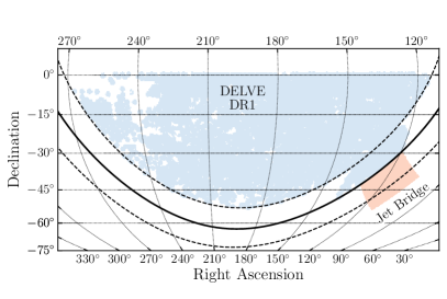
Figure 1: The DELVE DR1 region where our search was performed is shown in light blue. The additional region (the Jet Bridge) that was searched is shown as a light orange patch. The solid black line indicates the plane of the Milky Way ($b=0{}^{\circ}$) and the two dashed lines indicate $b=\pm 10{}^{\circ}$.

The DELVE DR1 dataset consists of $\sim$30,000 DECam exposures, with exposure times between $30\mathrm{\,s}<{\rm t_{exp}}<350\mathrm{\,s}$. Additionally, the following quality cuts were applied to individual exposures: a minimum cut on the effective exposure time scale factor $\mathrm{t_{eff}}>0.3$ (Neilsen et al., 2015) and a good astrometric solution relative to Gaia DR2 (For each exposure $>250$ astrometric matches, $\chi^{2}_{\rm astrom}<500$, where a match has $\Delta(\alpha)<150\mathrm{\,mas}$, and $\Delta(\delta)<150\mathrm{\,mas}$). All exposures were processed with the DES Data Management (DESDM) pipeline (Morganson et al., 2018), enabling sub-percent-level photometric accuracy by calibrating based on seasonally averaged bias and flat images and performing full-exposure sky background subtraction (Bernstein et al., 2018). Automatic source detection and photometric measurement is performed on each exposure using SExtractor and PSFex (Bertin & Arnouts, 1996; Bertin, 2011). Astrometric calibration was performed against Gaia DR2 using SCAMP (Bertin, 2006). Photometric zeropoints for each CCD were derived by performing a $1\mathrm{\,arcsec}$ match between the DELVE SExtractor catalogs and the ATLAS Refcat2 catalog (Tonry et al., 2018), and using transformation equations derived by comparing stars in ATLAS Refcat2 to calibrated stars from DES DR1 to convert the ATLAS Refcat2 measurements into the DECam griz-bandpass (Drlica-Wagner et al., 2021). The zeropoints derived from this processing were found to agree with the DES DR1 zeropoints with a scatter of $\lesssim 0.01\mathrm{\,mag}$. Dust extinction corrections were applied using extinction maps from Schlegel et al. (1998) assuming $R_{V}=3.1$ and a set of $R_{\lambda}$ coefficients derived by DES (DES Collaboration et al., 2018) including a normalization adjustment from Schlafly & Finkbeiner (2011). Hereafter, all quoted magnitudes have been corrected for interstellar extinction. For more details on the catalog creation and validation see Drlica-Wagner et al. (2021).

A high-quality stellar sample is selected based on the SExtractor quantity SPREAD_MODEL (Desai et al., 2012) measured in the DELVE g-band. Specifically, we select objects with $|\texttt{{SPREAD\_MODEL\_G}}|<0.003$. The performance of this classifier was evaluated by matching sources in the DELVE DR1 catalog with the W04 HSC-SSP PDR2 catalog (Aihara et al., 2019). For our analysis we choose a limiting magnitude of $g=23.1$ mag where the stellar completeness drops to $\sim 60\%$ and contamination rapidly rises to $\sim 40\%$ as estimated from the HSC catalog. For more information on morphological classification in this catalog see Drlica-Wagner et al. (2021). bright-end limit of 16th magnitude in the $g$-band is chosen to avoid saturation effects from bright stars. Additionally, since we are primarily interested in Main Sequence (MS) and Red Giant Branch (RGB) stars associated with old, metal-poor populations, we restrict the color range of our dataset to be $0.0<(g-r)_{0}<1.0$. Only objects passing the above morphological, magnitude, and color cuts are used in the following matched-filter analysis.

To account for missing survey coverage over our footprint, we quantify the sky area covered by DELVE DR1 in the form of HEALPix maps. These maps account for missing survey coverage, gaps associated with saturated stars and other instrumental signatures. They are created using the healsparse tool developed for the Legacy Survey of Space and Time (LSST) at the Vera C. Rubin Observatory, and its DECam implementation decasu to pixelize the geometry of each DECam CCD exposure. The coverage is calculated at a high resolution (nside =16384; ${\sim}\,0.01\mathrm{\,arcmin}^{2}$) and degraded to give a fraction of the lower resolution pixel area that is covered by the survey.

2.1 Gaia cross-match with DELVE DR1

To enable a characterization of the proper motion of the Jet stream, we use the Gaia EDR3 dataset (Gaia Collaboration et al., 2020). We begin by performing an angular cross match between the Gaia EDR3 dataset and DELVE DR1 with a matching radius of 0$\farcs$5. This results in a catalog containing ${\sim}\,143$ million sources. Subsequently, a number of quality cuts are applied. Nearby sources are removed by applying a parallax cut similar to Pace & Li (2019) of $\varpi-3\sigma_{\varpi}<0.05$. To remove sources with bad astrometric solutions we place a cut on the renormalized unit weight error (ruwe) of $\texttt{ruwe}<1.4$. Then, a cut on BP and RP excess is applied following equation 6 of Riello et al. (2020) ($|C^{\star}|<3\sigma_{C^{\star}})$. Additionally, only sources with $\texttt{astrom\_chi2\_al}<2$ are kept to avoid sources with bad astrometric fits in Gaia. We check that no known Active Galactic Nuclei (AGN) are in our sample by removing all sources that appear in the Gaia table gaiaedr3.agn_cross_id. Finally, we remove faint sources with $G>20$ mag to avoid contamination from stars with low signal-to-noise proper motion measurements. The resulting catalog is used for the analyses described in Sections 3.2 and 3.5.

3 Methods and Analysis

In this section we describe our procedure to fit the track, distance gradient, proper motion, and morphology of the Jet stream. We begin by performing an initial matched-filter selection for the Jet stream assuming the best-fit isochrone parameters and distance modulus from J18 (Section 3.1). This allows us to determine an initial estimate for the Jet stream track. We then select candidate BHB stars that lie along the track and are clustered in proper motion space to determine a distance gradient as a function of angular distance along the stream (Section 3.2). Then we create a new optimized matched-filter map of the Jet stream using the distance gradient of the candidate BHB stars, and refitting an isochrone to a Hess difference diagram (Section 3.3). This map is fit with a spline-based generative model to quantitatively characterize the track, intensity and width of the stream as a function of angular distance along the stream (Section 3.4). Finally, we select RGB and BHB stars consistent with being members of the Jet stream and fit a two component Gaussian mixture model to the selected stars determining the proper motion for the Jet stream including a linear gradient term (Section 3.5).

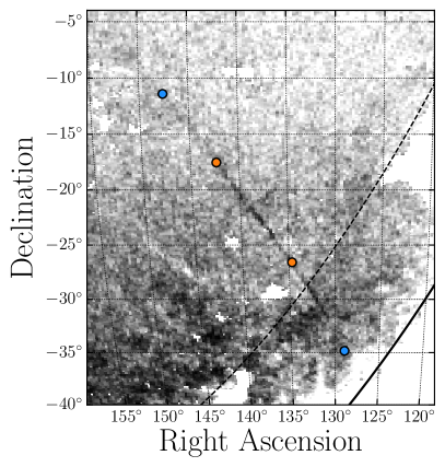
Figure 2: A stellar density map from the DELVE photometry showing the Jet stream at a distance modulus of $m-M=17.28$ ($\text{D}_{\odot}=28.6\mathrm{\,kpc}$). The orange points show the extent of the stream identified by Jethwa et al. (2018), and the blue points denote the new extent of the stream as detected in MSTO and BHB stars as determined in this study. The solid black line in the bottom right indicates the plane of the Milky Way ($b=0{}^{\circ}$), and the dashed line shows $b=10{}^{\circ}$.

3.1 Initial matched-filter Search

To investigate the Jet stream in DELVE DR1, we began by applying a matched-filter algorithm in color–magnitude space similar to Shipp et al. (2018, 2020). The matched-filter is derived from a Dotter et al. (2008) synthetic isochrone as implemented in ugali (Drlica-Wagner et al., 2020). Candidate MS stars are selected within a range of colors around the isochrone (Equation 4 in Shipp et al. 2018) taking into account photometric uncertainty. To select stars consistent with the Jet stream, we create a matched-filter based on the best-fit parameters (including distance modulus) taken from J18: an age of 12.1 Gyr, a metallicity of $\text{[Fe/H]}=$$-1.57$, and a distance modulus of $m-M=17.28\mathrm{\,mag}$.

Our selection is conducted using the DELVE DR1 catalog described in Section 2. Stars are selected using the matched-filter and then objects are pixelized into HEALPix pixels with nside = 512 (pixel area of ${\sim}\,0.01\deg^{2}$). The pixelized filtered map is corrected by the geometric survey coverage fraction for each pixel to account for survey incompleteness. This is done by dividing the number of counts in each pixel by the observed fraction of that pixel (Shipp et al., 2018). The coverage maps are created using the method described in Section 4.4 of DES Collaboration et al. (2021), and pixels with a coverage fraction less than 0.5 are removed from the analysis.

Figure 2 shows the results of this matched-filter selection. The Jet stream can be clearly seen to extend beyond the initial discovery bounds (marked by orange circles) in both directions. At high declination the stream becomes fainter and more diffuse and appears to fan out, and at lower declination an additional prominent component can be seen with obvious density variations.

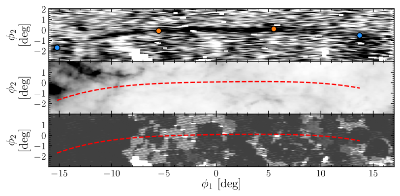
Figure 3: Top: Jet stream density after applying the same matched-filter as Figure 2. Additionally, deviations from great circle path $\phi_{2}=0{}^{\circ}$ are clearly seen. The orange points show the extent of the stream identified by Jethwa et al. (2018), and the blue points denote the new extent of the stream as detected in MSTO and BHB stars. For the range $\phi_{1}<-12.7{}^{\circ}$ or $>10{}^{\circ}$ the stream is only detected using BHB stars. Middle: SFD dust map of the same region. Bottom: Survey coverage map where the color shows the fraction of each pixel that is observed in the DELVE survey. White corresponds to observed fractions lower that 0.5 which are excluded from our analysis, and the greyscale ranges from light to dark with observed fractions of 0.7 to 1. The red dashed lines show the track of the Jet stream.

In absence of an obvious stream progenitor, we choose the stream-centered coordinate frame to be the same as J18 defined by pole $(\alpha_{pole},\delta_{pole})=64.983{}^{\circ},34.747{}^{\circ}$ and a $\phi_{1}$ center of $\phi_{1}=63{}^{\circ}$ ($\phi_{1},\phi_{2}=0{}^{\circ},0{}^{\circ}$ at $\alpha,\delta=138.62{}^{\circ},22.10{}^{\circ}$). We define the rotation matrix to convert $\alpha,\delta$ to $\phi_{1},\phi_{2}$ to be:

$$\boldsymbol{R}=\begin{bmatrix}-0.69798645&0.61127501&-0.37303856\\ -0.62615889&-0.26819784&0.73211677\\ 0.34747655&0.74458900&0.56995374\end{bmatrix}.$$ (1)

The top panel of Figure 3 shows the transformed matched-filter stellar density map. This map has been smoothed by a Gaussian kernel with a size of $\sigma=0.06{}^{\circ}$, and each column has been normalized to have the same median to correct for variable background stellar density along the field. The track of the stream clearly deviates from the great circle path defined by $\phi_{2}=0{}^{\circ}$. We fit a fourth-order polynomial to the peak intensity of the stream at each $\phi_{1}$ for the range $-14{}^{\circ}<\phi_{1}<14{}^{\circ}$ giving the following relation for $\phi_{2}$ as a function of $\phi_{1}$:

$$\phi_{2}(\phi_{1})= 0.07247+0.01475\times(\phi_{1})-0.00138\times(\phi_{1})^{2}$$ (2)

$$+0.00006\times(\phi_{1})^{3}-0.00002\times(\phi_{1})^{4}.$$

The middle panel of Figure 3 shows the Schlegel et al. (1998, SFD) dust map in the transformed frame of Jet, and the bottom panel shows the survey coverage map in this region. These two maps demonstrate that the detection of the Jet stream does not correlate with any linear extinction features or variations in survey coverage.

3.2 Distance Gradient

Using the DELVE DR1 catalog cross-matched with Gaia EDR3 (Section 2.1), we identify candidate BHB stars and use them to measure a distance gradient along the Jet stream. BHB stars are useful for determining a distance gradient because of the tight color-luminosity relation that allows for distance estimates with ${\sim}\,10\%$ uncertainty to an individual BHB star (Deason et al., 2011). To determine a distance gradient we use a similar method to Li et al. (2020) who use BHB stars to measure the distance gradient of the ATLAS-Aliqa Uma stream. For the Jet stream, the gradient derived from BHB stars can be used to refine the matched-filter selection from Section 3.1, make a reflex-corrected proper motion measurement in Section 3.5, and improve dynamical modeling of the stream (Section 4). Hereafter, all proper motions ($\mu_{\phi_{1}}^{\star},\mu_{\phi_{2}}$) are assumed to be reflex corrected unless explicitly stated otherwise. We select probable BHB stars along the track of the stream using a few criteria. Initially we select all sources with $-12{}^{\circ}<\phi_{1}<10{}^{\circ}$ and separation from the stream track $\Delta\phi_{2}<0.5{}^{\circ}$ ( Equation 2). Then, a color cut is applied to select blue stars keeping only sources with $(g-r)_{0}$ between $-$0.3 and 0.0 mag. We then cut all sources with $g$-band magnitudes less than 17.0 mag or greater than 18.5 mag to reduce contamination from the Milky Way foreground. For each candidate we derive an estimate of its distance modulus, $m-M$, by assuming it is a BHB star and using the relation for $M_{g}$ vs. $(g-r)_{0}$ from Belokurov & Koposov (2016).

To further remove contaminant stars from the Jet stream BHB stellar sample, we use the Gaia EDR3 proper motions of candidate BHB stars along the Jet stream track. We use the distance estimated for each BHB star to correct their proper motions for the solar reflex motion assuming a relative velocity of the Sun to the Galactic standard of rest to be $(U_{\odot},V_{\odot},W_{\odot})=(11.1,240.0,7.3)\text{ km}\text{/s}$ (Bovy et al., 2012). Figure 4 (left panel) shows the resulting measured proper motion of our BHB candidate sample. The proper motion signal of the Jet stream is seen at $(\mu_{\phi_{1}}^{\star},\mu_{\phi_{2}}){\sim}\,(-1,0)$ mas/yr, where we define $\mu^{\star}_{\phi_{1}}=\mu_{\phi_{1}}\cos(\phi_{2})$. Additionally, contributions due to the Milky Way foreground and stellar halo are seen at $(\mu_{\phi_{1}}^{\star},\mu_{\phi_{2}}){\sim}\,(0.5,2)$ and $(0.5,0)$ mas/yr respectively The BHB candidates within the green box are selected as likely members of the Jet stream to be used to estimate the distance gradient. Figure 4 (right panels) shows on-sky positions and distances of the likely member candidate BHB stars.

Using these derived distances and assuming an uncertainty of 0.1 mag on the distance modulus for each BHB star (Deason et al., 2011), we fit for the distance modulus as a function of position along the stream using a simple linear fit. We find the following relation for the distance modulus as a function of $\phi_{1}$ along the Jet stream,

$$(m-M)=17.45-0.014\times(\phi_{1}).$$ (3)

The heliocentric distance of the Jet stream is found to vary from $26\mathrm{\,kpc}$ to $34.5\mathrm{\,kpc}$ over its observed length with a gradient of $-0.2$ kpc/deg.

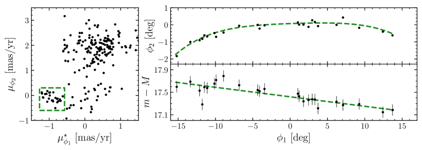
Figure 4: Left: proper motions of candidate BHB stars along the Jet stream. The green box shows our proper motion selection for likely members. Contributions from the Milky Way foreground and stellar halo are seen at $(\mu_{\phi_{1}}^{\star},\mu_{\phi_{2}})\sim(0.5,2)$ and $(0.5,0)$ mas/yr respectively Right: on-sky distribution (top) and distances modulus (bottom) of candidate BHB stars that are likely associated with the Jet stream. The matched-filter stream track (Equation 2 is shown as green dashed line on the top plot, and the linear fit on distance modulus, $(m-M)$, of the candidate BHB stars (Equation 3) is shown as a green dashed line on the bottom plot.

3.3 Creation of optimized matched-filter map

We next use our measured distance gradient to find a best-fit isochrone, and create an optimized matched-filter map to study the morphology of the stream. We begin by creating a Hess difference diagram shown in Figure 5. This is done by selecting stars along the stream track with $-11{}^{\circ}<\phi_{1}<-8{}^{\circ}$ as well as stars with $-5{}^{\circ}<\phi_{1}<6{}^{\circ}$, excluding the area around the observed under-density in the stream at $\phi_{1}\sim-6.5{}^{\circ}$ to increase signal-to-noise. In $\phi_{2}$ we select stars within 2 times the observed width of the stream ($w$) as a function of $\phi_{1}$ (the width is derived in Section 3.4). At $\phi_{1}=0$ we find a width of $w=0.16{}^{\circ}$ and this value varies from $w=0.13{}^{\circ}$ at $\phi_{1}=-11{}^{\circ}$ to $w=0.19{}^{\circ}$ at $\phi_{1}=6{}^{\circ}$. Additionally, a background region is selected to be along the same $\phi_{1}$ range but above and below the stream, with $1{}^{\circ}<|\phi_{2}|<2{}^{\circ}$. For the stars in each of these regions we compute the absolute $g$-band magnitude ($M_{g}$) assuming a distance modulus derived from the observed BHB stars’ gradient (Equation 3). Then we select only stars with $M_{g}<5.47$; this corresponds to the faint limit of our catalog ($g_{0}=23.1$) at $\phi_{1}=-13{}^{\circ}$, the most distant portion of the detected stream. This absolute magnitude selection ensures that the observed density variations in the matched-filter map are not affected by the survey completeness. We then create binned color–magnitude diagrams (CMDs) for the on-stream and background selections and subtract the background from the on-stream region correcting for relative areas. The result of this process is shown in Figure 5.

Next we fit an isochrone to this Hess difference diagram using a similar methodology to Shipp et al. (2018). Briefly, we model the observed binned CMD of the stream region as a linear combination of the background region and a stellar population following a Dotter et al. (2008) isochrone. Then we compute the likelihood that the binned CMD is a Poisson sample of the model. This likelihood is then sampled using emcee (Foreman-Mackey et al., 2013). We find a best-fit isochrone consistent with the J18 result and distance modulus in strong agreement with the distance derived from candidate BHB stars ($(m-M)_{MS}-(m-M)_{BHB}=0.01^{+0.05}_{-0.05}$).

Since we find consistent results, we use the J18 isochrone to create an optimized matched-filter that is used in Section 3.4 to quantitatively characterize distance variation. This map covers the region defined by $-16{}^{\circ}\leq\phi_{1}\leq 17{}^{\circ}$, and $-3{}^{\circ}\leq\phi_{1}\leq 1{}^{\circ}$. We choose a pixel size of 0.2 deg in $\phi_{1}$ and 0.05 deg in $\phi_{2}$. The distance modulus of the matched-filter follows Equation 3. The result of this more optimal matched-filter is shown in the top panel of Figure 6. We note that while the image in Figure 6 has been smoothed with a 0.08 deg Gaussian kernel, we do not apply any smoothing when fitting our model to the stream data.

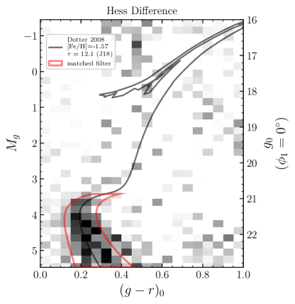
Figure 5: Hess difference diagram created by subtracting a background region from the on-stream region. The main sequence of the Jet stream is clearly seen. The Dotter et al. (2008) isochrone we use for our analysis with a metallicity of [Fe/H]=$-1.57$ and age of $\tau=12.1\mathrm{\,Gyr}$ is shown as a solid black line. The red line shows the matched-filter used to create the optimized map shown in the top row of Figure 6. The left y-axis shows the absolute magnitude of sources and the right y-axis shows the corresponding apparent magnitude at $\phi_{1}=0{}^{\circ}$.

3.4 Fitting Stream Morphology

To quantitatively characterize the observed features of the stream morphology we use a generative stream model developed by Koposov et al. (2019) and Li et al. (2020), which is similar to that of Erkal et al. (2017). This model uses natural cubic splines with different numbers of nodes to describe stream properties. This model is implemented in STAN (Carpenter et al., 2017) and is fit to the data using the Hamiltonian Monte Carlo No-U-Turn Sampler (NUTS) to efficiently sample the high dimensional parameter space.

The stream is modeled by a single Gaussian in $\phi_{2}$ with central intensity, width, and track that are allowed to vary as functions of $\phi_{1}$. The parameters of the model are $\mathcal{I}(\phi_{1})$, $w(\phi_{1}),\,\Phi_{2}(\phi_{1}),\,\mathcal{B}_{1}(\phi_{1}),\,\mathcal{B}_{2}(\phi_{1}),$ and $\mathcal{B}_{3}(\phi_{1})$, which describe the logarithm of the stream central intensity, the logarithm of the stream width, the stream track, the log-background density, the slope of the log-background density, and the quadratic term of the log-background density, respectively. For more details see Koposov et al. (2019) (Section 3.1 and equation 2) The model is fit to the binned matched-filter data described above using Equation 3 to describe the distance modulus as a function of $\phi_{1}$. We assume the number of stars in an individual pixel of the matched-filter map is a Poisson sample of the model density at that location.

Following Li et al. (2020), we use Bayesian optimization to determine model complexity in a data-driven way. In particular, the number of nodes for all parameters except the stream width are hyper-parameters of this model, and they are determined through model selection. Where Bayesian optimization (Gonzalez et al., 2016; The GPyOpt authors, 2016) of the cross-validated ($k=3$) log-likelihood function is used. For the parameters [$\mathcal{I}(\phi_{1})$, $w(\phi_{1})$, $\Phi_{2}(\phi_{1})$, $\mathcal{B}_{0}(\phi_{1})$, $\mathcal{B}_{1}(\phi_{1})$, $\mathcal{B}_{2}(\phi_{1})$] we find the optimal number of nodes to be [11, 3, 8, 28, 25, 5], respectively. For each parameter, the range of allowable nodes is 3 to 30 except for the width, $w(\phi_{1})$, and quadratic term of the log-background density, $\mathcal{B}_{3}(\phi_{1})$, which have their maximum number of nodes constrained to 15 and 10, respectively. The model is run for 1500 iterations with the first 700 discarded as burn in.

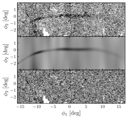
Figure 6: Modeling the track, width, and intensity of the Jet stream from DELVE DR1 photometric data. Top: The density of stars that pass the optimized matched-filter selection that takes into account the observed distance gradient in the region of the Jet stream. Middle: The maximum a posteriori (MAP) model of the data shown in the top panel containing both stream and background components. Bottom: The residual density map showing the observed density minus the model.

The results of the model fit are shown in Figures 6 and 7. For Figure 6 the top row shows the observed matched-filter map, the best-fit model is shown on the second in the same color scale, and the residual of the model subtracted from the data is shown on the bottom row. The key features captured by this model are the variations in the density of stars. A large gap can be seen at $\phi_{1}=-6{}^{\circ}$, and peaks in the intensity are found at at $\phi_{1}=-9{}^{\circ},-2.5{}^{\circ}$ and $4{}^{\circ}$. The model does not capture all of the observed small-scale substructure. In particular, the off-track structure seen crossing the stream at $\phi_{1}=-12$ or the overdensity above the stream at $\phi_{1}=5\,{}^{\circ}$ are discussed in more detail in Section 5.2.

The nature of the on-stream structure can be better evaluated by looking at the extracted stream parameters in Figure 7. These plots show the stream surface brightness, the on-sky track, stream width and linear density. In each panel, the best-fit value calculated as the maximum a posteriori (MAP) of the posterior for each parameter as a function of $\phi_{1}$ is shown as a black line, and the 68% containment peak interval is shown as the blue shaded region. The apparent width of the stream increases with $\phi_{1}$, consistent with expected projection effects due to a constant width and the observed distance gradient. This is supported by the relatively constant linear density over large scales.

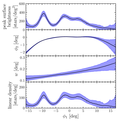
Figure 7: Measurement of Jet stream parameters as a function of position along the stream ($\phi_{1}$) as derived from modeling the DELVE DR1 stellar density maps. From top to bottom are stream surface brightness, stream track, stream width, and linear density. The shaded area shows the 68% containment peak interval, and the black line shows the best-fit estimate of each parameter.

3.5 Proper Motion of the Jet Stream

In this section, we use the cross-matched DELVE DR1 and Gaia EDR3 catalog to measure the proper motion of the Jet stream. In Section 3.2 we demonstrated that the proper motion signature of BHB stars could be clearly separated from the Milky Way foreground. We seek to extend our analysis to the full stellar population of Jet, applying several additional physically motivated cuts to reduce Milky Way foreground contamination. Then we perform a Gaussian mixture model fit with stream and Milky Way components to measure the proper motion of Jet.

3.5.1 Data Preparation

Starting with the stellar catalog from Section 2.1, we apply several cuts to reduce Milky Way contamination in our sample and to highlight the Jet stream population. These cuts are depicted visually in the left two panels of Figure 8. The following selection process largely follows the methodology set out by Shipp et al. (2019) and Li et al. (2019).

We begin by calculating the absolute magnitude in the $g$-band ($M_{g}$) for each star assuming a distance given by the fit to the BHB stars (Equation 3; $m-M(\phi_{1})$). A magnitude cut is made keeping only sources with $M_{g}<2$ to remove faint sources with large proper motion uncertainties. Then, a color–magnitude selection is applied selecting stars in $(g-r)_{0}$ vs. $M_{g}$ color–magnitude space (Fig. 8 left panel). RGB stars are selected based on the Dotter et al. (2008) isochrone used in Section 3.1. We select stars that meet either of the following conditions:

$$-0.08 \leq (g-r)_{0}- (g-r)_{\rm Dotter} \leq 0.02$$ (4)

$$-0.5 \leq g_{0}- (g_{0})_{\rm Dotter} \leq 0.5.$$

where $(g-r)_{\rm Dotter}$ is the isochrone color at a given observed magnitude and $(g_{0})_{\rm Dotter}$ is the isochrone magnitude at a given observed color. Next, we applied a $(g-r)_{0}$ vs. $(r-i)_{0}$ color–color cut to select metal poor stars based on an empirical stellar locus that is derived from dereddened DES data (second panel; Pace & Li, 2019; Li et al., 2018). This locus gives the median $(r-i)_{0}$ colors for each $(g-r)_{0}$ bin, For each star we compute $\Delta_{ri}=(r-i)_{0}-(r-i)_{\rm med}$ where $(r-i)_{0}$ is the observed color of a star and $(r-i)_{\rm med}$ is the median $(r-i)_{0}$ color of stars with the same $(g-r)_{0}$ color taken from the empirical stellar locus. Only stars within $-0.02<\Delta_{ri}<0.1$ are kept. Finally, a spatial cut is applied only keeping stars within $3\times w(\phi_{1})$ of the stream track where $w(\phi_{1})$ is the stream width and track taken from the modeling in Section 3.4.

To select candidate horizontal branch members for the proper motion fit, we use an empirical horizontal branch of M92 initially derived in Belokurov et al. (2007) and transformed to the DES photometric system (Li et al., 2019; Pace & Li, 2019). We select stars with $(g-r)_{0}$ colors within $\pm 0.1$ mag and $M_{g}$ within $\pm 0.5$ mag of the empirical horizontal branch.

After applying these cuts, we perform a reflex correction on the proper motion measurements of the remaining sources (assuming the distance fit from Equation 3). The proper motion signal of Jet is easily identified in the third panel of Figure 8 as the overdensity at $(\mu_{\phi_{1}}^{\star},\mu_{\phi_{2}})\sim(-1,0)$  mas/yr. To quantitatively measure the proper motion and any gradient in the proper motion, we use a Gaussian mixture model based analysis described in the following section.

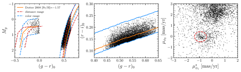
Figure 8: Selection of stars used to measure the proper motion of the Jet stream. Left: A color–magnitude diagram demonstrating the selection applied to the data. The orange lines show the empirical M92 horizontal branch and Dotter isochrone ($[\text{Fe/H}]=$$-1.57$) used to select data. The blue dashed lines show our selection range in distance, and the red dashed lines our selection range in color. Center: A color-color plot showing our selection range in blue around an empirical stellar locus of dereddened DES photometry in orange. Right: Proper motion in stream coordinates of the sample of stars passing all selection cuts. The signal from the Jet stream is easily seen at $(\mu_{\phi_{1}}^{\star},\mu_{\phi_{2}})\sim(-1,0)$ mas/yr (circled in red).

3.5.2 Mixture Model

To determine the proper motion of the Jet stream, we use a simple mixture model consisting of Gaussian distributions for the stream and Milky Way foreground. The fit is performed on the candidate RGB and BHB stellar sample defined in the previous section and shown in the right panel of Figure 8. The likelihood and fitting methodology follows that of Pace & Li (2019) and Shipp et al. (2019). The complete likelihood is given by:

$$\mathcal{L}=(1-\lambda)\mathcal{L}_{\rm Jet}+\lambda\mathcal{L}_{\rm MW}$$ (5)

where $\mathcal{L}_{\rm Jet}$ is the likelihood that a star belongs to the Jet stream component, and $\mathcal{L}_{\rm MW}$ refers to the likelihood that a star belongs to the Milky Way foreground component. The fraction of stars that belong to the Milky Way component is denoted by $\lambda$. Each likelihood term is made up of the product of both spatial and proper motion likelihoods,

$$\mathcal{L}_{\rm Jet/MW}=\mathcal{L}_{\rm spatial}\;\mathcal{L}_{\rm PM}.$$ (6)

For the stream spatial component we use the results from Section 3.4 for the stream track, $\Phi_{2}(\phi_{1})$, and width, $w(\phi_{1})$, assuming the stream follows a Gaussian distribution in $\phi_{2}$ around this track (i.e. $\phi_{2,\text{obs}}-\Phi_{2}(\phi_{1})$ with standard deviation $w(\phi_{1})$. The Milky Way spatial component is assumed to be uniform.

$$\mathcal{L}_{\rm spatial}=\begin{cases}\mathcal{N}(\phi_{2}\,|\,\Phi_{2}(\phi_{1}),w_{\mathrm{Jet}})&\text{Jet component}\\ \mathrm{Uniform}&\text{MW component}\\ \end{cases}$$ (7)

The proper motion term of the likelihood is modeled by the combination of several multivariate Gaussians.

Each Gaussian is defined to have a mean proper motion vector $\boldsymbol{\chi}$ given by $\boldsymbol{\chi}=(\mu_{\phi_{1},Jet}^{\star}(\phi_{1}),\mu_{\phi_{2},Jet}(\phi_{1}))$. We model both components of $\boldsymbol{\chi}$ as a linear functions of $\phi_{1}$. The covariance, $\boldsymbol{C}$, is defined by an observational error component and an intrinsic component:

$$\boldsymbol{C} =\boldsymbol{C}_{obs}+\boldsymbol{C}_{intrinsic}$$

$$=\begin{bmatrix}\epsilon_{\mu_{\phi_{1}}\,\cos\phi_{2}}^{2}&\epsilon_{\mu_{\phi_{1}}\,\cos\phi_{2}\times\mu_{\phi_{2}}}\\ \epsilon_{\mu_{\phi_{1}}\,\cos\phi_{2}\times\mu_{\phi_{2}}}&\epsilon_{\mu_{\phi_{2}}}^{2}\ \end{bmatrix}+$$ (8)

$$\quad\;\begin{bmatrix}\sigma_{\mu_{\phi_{1}}\,\cos\phi_{2}}^{2}&\sigma_{\mu_{\phi_{1}}\,\cos\phi_{2}}\times\sigma_{\mu_{\phi_{2}}}\times\rho\\ \sigma_{\mu_{\phi_{1}}\,\cos\phi_{2}}\times\sigma_{\mu_{\phi_{2}}}\times\rho&\sigma_{\mu_{\phi_{2}}}^{2}\\ \end{bmatrix}$$

where $\epsilon$ represents the proper motion errors, $\sigma$ is the intrinsic proper motion dispersions, and $\rho$ is a correlation term. For the stream component, the intrinsic dispersion is assumed to be $5\mathrm{\,km}/\mathrm{\,s}$ which at the distance of the stream corresponds to $\sim 0.04\mathrm{\,mas}/\mathrm{\,yr}$ and the correlation terms are assumed to be zero.

The model then has 9 free parameters: The systemic proper motions of the stream measured at $\phi_{1}=0{}^{\circ}$ ($\bar{\mu}_{\phi_{1}}\cos(\phi_{2}),\bar{\mu}_{\phi_{2}}$), the proper motion gradients in each coordinate direction for the stream ($d\mu_{\phi_{1}}/d\phi_{1},d\mu_{\phi_{2}}/d\phi_{1}$) in units of $\mathrm{\,mas}/10{}^{\circ}$, the mean proper motion of the Milky Way foreground Gaussian ($\mu_{\phi_{1}\,{\rm MW}},\mu_{\phi_{2}\,{\rm MW}}$), the dispersion of the Milky Way foreground Gaussian ($\sigma_{\phi_{1}\,{\rm MW}},\sigma_{\phi_{2}\,{\rm MW}}$), and the fraction of stars that belong to the stream component ($\lambda$). The proper motion of the stream component as a function of $\phi_{1}$ is given by

$$\mu_{\phi_{1},\mathrm{Jet}}(\phi_{1}) =\bar{\mu}_{\phi_{1}}+\,\frac{d\mu_{\phi_{1}}}{d\phi_{1}}\times(\phi_{1}/10\deg)$$ (9)

$$\mu_{\phi_{2},\mathrm{Jet}}(\phi_{1}) =\bar{\mu}_{\phi_{2}}+\,\frac{d\mu_{\phi_{2}}}{d\phi_{1}}\times(\phi_{1}/10\deg).$$

The total proper motion likelihood is then given by

$$\mathcal{L}_{\rm PM}=\sum_{N=1}^{k}\mathcal{N}((\boldsymbol{\mu}_{\phi_{1},obs}^{\star},\boldsymbol{\mu}_{\phi_{2},obs})_{N}\,|\,\boldsymbol{\chi}_{true,N}\;,\boldsymbol{C_{N}}).$$ (10)

Parameter inference is conducted using a Hamiltonian Monte Carlo No-U-Turn Sampler (NUTS) implemented in STAN (Carpenter et al., 2017). We use 10 parallel chains with 2000 iterations each (1000 of the iterations are discarded as a burn in). Convergence is verified using the Gelman-Rubin $\hat{R}<1.1$ diagnostic (Gelman & Rubin, 1992).

The results of our fit are listed in Table 1. We find the results from the mixture model  ($\bar{\mu}_{\phi_{1},\mathrm{Jet}}^{\star},\bar{\mu}_{\phi_{2},\mathrm{Jet}})=(-0.933\pm 0.018,-0.023\pm 0.016)$ mas/yr, which agrees with our rough estimate from the observed overdensity of candidate BHB stars in Section 3.2. The $\bar{\mu}_{\phi_{2}}$ value is near zero as expected for a stable stream that has not been heavily perturbed. We detect gradients in both proper motion coordinates that are similar in magnitude. Based on these results, the tangential velocity of the Jet stream at $\phi_{1}=0{}^{\circ}$ is $v_{tan}=195\pm 3$ km/s.

A membership probability is calculated for each star by taking the ratio of the stream likelihood to the total likelihood: $p_{mem}=\lambda\mathcal{L}_{\mathrm{Jet}}/(\lambda\mathcal{L}_{\rm Jet}+(1-\lambda)\mathcal{L}_{\rm MW})$. To determine the value of $p_{mem,i}$ for each star we calculate $p_{mem}$ for each point in the posterior of our fit and take $p_{mem,i}$ to be the median of the calculated values for each star. A star is then considered a high (medium) probability member if $p_{mem,i}>0.8\;(0.5)$. For our sample, $89\;(97)$ candidate RGB stars and $28\;(28)$ candidate BHB stars pass this criterion.

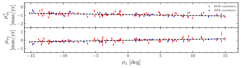
Figure 9: Proper motion of high probability member RGB (red) and BHB (blue) stars ($p_{mem}>0.8$). Additionally the line of best-fit proper motion is shown as a black dashed line. All the BHB stars used to measure the distance gradient are also high probability members.

The proper motion of the high probability stars are shown in Figure 9 along with lines showing the best-fit stream proper motion ($\bar{\mu}_{\phi_{1}}^{\star}(\phi_{1}),\bar{\mu}_{\phi_{2}}(\phi_{1}))$ from our analysis. The BHB stellar sample (blue points) is very similar to the sample selected by a rough cut in Figure 4, and it can be seen that these stars closely follow the proper motion gradient ($d\mu/d\phi_{1}$) found in our analysis. In Appendix A, we include Table A.1 that contains the properties of all candidate BHB and RGB stars with membership probability ($p_{mem}$) higher than 10%. With the current dataset we are only able to fit for linear evolution of the proper motion with $\phi_{1}$, but with future spectroscopic datasets can test for a more complex evolution of the proper motion as a function of $\phi_{1}$ (e.g., quadratic).

Previous studies such as Shipp et al. (2019) have looked for signs of large scale perturbation of stellar streams from the influence of the LMC or Milky Way bar (Li et al., 2018; Erkal et al., 2018; Koposov et al., 2019; Vasiliev et al., 2021). Evidence of these interactions sometimes appears as a mismatch between the proper motion of the stream ($\mu_{\phi_{2}}/\mu_{\phi_{1}}$) and the derivative of the stream track ($d\phi_{2}/d\phi_{1}$) (Erkal et al., 2019). In the case of Jet, we find that the ratio of the proper motions to the stream track ($\mu_{\phi_{2}}/\mu_{\phi_{1}})/(d\phi_{2}/d\phi_{1}$) has an average value of $2.00\pm 1.18$ over the extent of the stream. This is consistent with a value of one which indicates the proper motions are largely aligned with the track of the stream.

Table 1: Results of the proper motion fit in reflex corrected proper motion coordinates

Parameter	Value	Prior	Range	Units
$\bar{\mu}_{\phi_{1}}^{\star}$	$-0.933\pm 0.018$	Uniform	-10,10	mas/yr
$\bar{\mu}_{\phi_{2}}$	$-0.023\pm 0.016$	Uniform	-10,10	mas/yr
$d\mu_{\phi_{1}}^{\star}/d\phi_{1}$	$-0.109\pm 0.030$	Uniform	-3,3	mas/yr/10 deg
$d\mu_{\phi_{2}}/d\phi_{1}$	$0.120\pm 0.021$	Uniform	3,3	mas/yr/10 deg
$\lambda$	$0.086\pm 0.011$	Uniform	0,1

4 Dynamical Modeling

Using our measurements of the stream track, distance, and proper motion, we can fit a dynamical model to the data. The Jet stream is modeled in the same method as Erkal et al. (2019) and Shipp et al. (2021). We make use of the modified Lagrange Cloud Stripping (mLCS) technique developed in Gibbons et al. (2014) adapted to include the total gravitational potential of the stream progenitor, the Milky Way, and the LMC. Following Erkal et al. (2019), the Milky Way and LMC are modeled as independent particles with their respective gravitational potentials which allows us to capture the response of the Milky Way to the LMC. The Milky Way potential is modeled with 6 axisymmetric components, namely bulge, dark matter halo, thin and thick stellar disk, and HI and molecular gas disk components following McMillan (2017). Following Shipp et al. (2021), we normalize the Milky Way potential to the realization of the McMillan (2017) potential that yields the best-fit from the ATLAS data ($M_{\rm MW}=8.3\times 10^{11}M_{\rm\odot}$; Li et al., 2020). We evaluate the acceleration from the potential using galpot (Dehnen & Binney, 1998). We take the Sun’s position ($R_{0}=8.23$ kpc) and 3D velocity, ($\text{U}_{\odot},\text{V}_{\odot},\text{W}_{\odot})=(8.6,232.8,7.1)$ km/s, from McMillan (2017).

We model the mass distribution of the LMC as a stellar disk and a dark matter halo. The stellar disk is modelled as a Miyamoto-Nagai disk (Miyamoto & Nagai, 1975) with a mass of $3\times 10^{9}M_{\odot}$, a scale radius of $1.5$ kpc, and a scale height of $0.3$ kpc. The orientation of the LMC disk matches the measurement of van der Marel & Kallivayalil (2014). The LMC’s dark matter halo is modelled as a Hernquist profile (Hernquist, 1990). We fix the total infall mass of the LMC to $1.5\times 10^{11}\mathrm{\,M_{\odot}}$, consistent with the value derived in Erkal et al. (2019) and Shipp et al. (2021). We fix the scale radius to match the circular velocity measurement of $91.7$ km/s at $8.7$ kpc from van der Marel & Kallivayalil (2014). Note that this is in agreement with more recent measurements of the LMC’s circular velocity (e.g., Cullinane et al., 2020). We account for the dynamical friction of the Milky Way on the LMC using the results of Jethwa et al. (2016). We also fix the LMC’s present-day proper motion, distance, and radial velocity to measured values (Kallivayalil et al., 2013; Pietrzyński et al., 2013; van der Marel et al., 2002). The LMC mass remains fixed throughout each simulation.

We model the potential of the Jet stream’s progenitor as a Plummer sphere (Plummer, 1911) with a mass and scale radius chosen to match the observed stream width. During the course of tidal disruption, the progenitor’s mass decreases linearly in time to account for tidal stripping. Since Jet does not have a known progenitor, we assume that the progenitor has completely disrupted, i.e., that its present day mass is zero. Furthermore, we assume that the remnant of the progenitor is located at $\phi_{1}=0{}^{\circ}$.

We calculate the likelihood for the stream model by producing a mock observation of a simulated stream and comparing it with the data described in the previous sections. For each stream model, we calculate the track on the sky, the radial velocity, the proper motions in $\phi_{1}$ and $\phi_{2}$, and the distance as functions of $\phi_{1}$, the observed angle along the stream.

We assign the mass of the progenitor in order to reproduce the observed width of the stream. Our best-fit model uses a progenitor mass of $M_{\rm prog}=2\times 10^{4}\mathrm{\,M_{\odot}}$, and a Plummer scale radius of $r_{\rm plum}=10\mathrm{\,pc}$. We note that these values are highly dependent on the location of the progenitor.

We perform a Markov Chain Monte Carlo (MCMC) fit using emcee (Foreman-Mackey et al., 2013). Our model includes 5 free parameters. We fit the present-day progenitor $\phi_{2}$ position, distance, radial velocity, and proper motion. The prior distributions on each parameter are listed in Table 2. The position of the progenitor along the stream is fixed to $\phi_{1}=0{}^{\circ}$ (i.e., the middle of the stream’s observed extent). We show the Jet data and the best-fit stream models in Figure 10. In each panel we show the observations in red, and simulated stream in blue. The radial velocity panel contains no observations, but can be used to predict the radial velocity of the stream. We find the best-fit model is a good fit to the observations of the distance modulus, stream track and proper motions.

We have tried fits that include/exclude the effect of the LMC and Milky Way bar. For the Milky Way bar we assume an analytic model with the same parameters as used in Li et al. (2020) (described in their Section 5.2.1) and Shipp et al. (2021). For both cases, the LMC and Milky Way bar, we find that it is unlikely that the Jet stream has been significantly affected by these substructures.

This model emphasizes some of the observed features of the Jet stream discussed in Sections 3.4 and 3.5. In particular, we note the observed curvature of the stream track away from $\phi_{2}=0{}^{\circ}$ is due both to Galactic parallax and the non-spherical potential of the MW. None of the intensity features gaps/peaks are seen in the model, and we also fail to replicate the off-track features seen in the photometry. Additionally, this model predicts a stream component in the Jet Bridge region (figure 1) that is not detected in our search. This non-detection is likely due to the increased Milky Way foreground contamination and reddening in this region

Table 2: Priors on the dynamical model

Parameter	Prior	Range	Units	Description
$\phi_{\rm 2,prog}$	Uniform	(-1, 1)	deg	Location of the progenitor perpendicular to the stream track.
$\mu_{\rm\alpha,prog},\mu_{\rm\delta,prog}$	Uniform	(-10, 10)	mas/yr	Reflex-corrected proper motion of the progenitor.
$v_{\rm r,prog}$	Uniform	(-500, 500)	km/s	Radial velocity of the progenitor.
$(m-M)_{\rm prog}$	Normal	$(m-M)_{0}\pm 0.2$	mag	Distance modulus of the progenitor.
$\phi_{\rm 1,prog}$	Fixed	0	deg	Location of the progenitor along the stream track.
$M_{\rm LMC}$	Fixed	$1.5\times 10^{11}$	$\mathrm{\,M_{\odot}}$	Total mass of the LMC.
$\mu_{\rm\alpha,LMC}$	Normal	$1.91$	mas/yr	Proper motion of the LMC in RA.
$\mu_{\rm\delta,LMC}$	Normal	$0.229$	mas/yr	Proper motion of the LMC in Dec.
$v_{\rm r,LMC}$	Normal	$262.2$	km/s	Radial velocity of the LMC.
$d_{\rm LMC}$	Normal	$49970.0$	pc	Distance of the LMC.

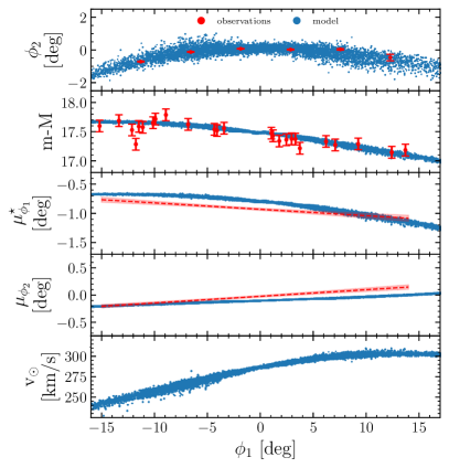
Figure 10: Best-fit stream model to the Jet stream. In each row the dark blue points show the best-fit stream model and the red points show the observations to which the model was fit. First row: the on-sky distribution of the stream. Second row: the distance modulus of the stream. Third and Fourth rows: The reflex-corrected proper motions of the stream in $\phi_{1}$ and $\phi_{2}$ respectively. Fifth row: predicted heliocentric velocities of the stream.

5 Discussion

5.1 Properties of the Jet stream

The Jet stream is now detected from $-15.2{}^{\circ}\leq\phi_{1}\leq 13.7{}^{\circ}$ increasing its known length from $\sim 11{}^{\circ}$ to nearly $29{}^{\circ}$. For $\sim 23{}^{\circ}$ ($-13{}^{\circ}\leq\phi_{1}\leq 10{}^{\circ}$) the main sequence turn off of the stream is strongly detected in the DELVE photometry; at $\phi_{1}<-13{}^{\circ}$ and $>10{}^{\circ}$ the intensity of the stream decreases greatly, and so is only significantly detected using BHB and RGB stars with measured proper motions. At observed distances ranging from $\sim 26-34.5\mathrm{\,kpc}$, the stream has a physical length of 16 kpc, with a strong photometric detection covering 13.4 kpc. This makes the extent of the Jet stream comparable to the kinematically cold Phoenix, ATLAS, and GD-1 streams (Balbinot et al., 2016; Koposov et al., 2014; Grillmair & Dionatos, 2006), which span ${\sim}\,5\mathrm{\,kpc}$ ($13.6{}^{\circ}$; Shipp et al., 2018), ${\sim}\,12\mathrm{\,kpc}$ ($34{}^{\circ}$ including Aliqa Uma; Li et al., 2020) and ${\sim}\,15.4\mathrm{\,kpc}$ (${\sim}\,100{}^{\circ}$; de Boer et al., 2020; Webb & Bovy, 2019; Price-Whelan & Bonaca, 2018; Malhan et al., 2018), respectively. Our dynamical models place Jet on a retrograde orbit with a pericenter of $12.7\mathrm{\,kpc}$ which is comparable to the pericenters of Phoenix (${\sim}\,13\mathrm{\,kpc}$; Wan et al., 2020) ATLAS ($13.3\mathrm{\,kpc}$; Li et al., 2020), Kshir (${\sim}\,14\mathrm{\,kpc}$; Malhan et al., 2019), and GD-1 (${\sim}\,14\mathrm{\,kpc}$; Koposov et al., 2010; Malhan & Ibata, 2019).

As discussed in Section 3.5, the proper motion of the Jet stream members and the observed track of the stream are fairly well aligned, suggesting that the Jet stream has not been strongly perturbed perpendicular to the line of sight from interactions with large Milky Way substructures. However, perturbations in the radial or track direction are difficult to measure from proper motion alone.

5.2 Small-Scale Features

This detailed view of the Jet stream has started to reveal its complexity, adding it to the group of streams that show small-scale features (e.g., Erkal et al., 2017; Price-Whelan & Bonaca, 2018; Li et al., 2020; Caldwell et al., 2020). Most noticeably, a ${\sim}\,4{}^{\circ}$ gap in the stream is seen centered on $\phi_{1}=-6{}^{\circ}$ extending from -. This structure may be due to interactions between the Jet stream and its environment (e.g., a dark matter subhalo passing by and perturbing the stream), or the environment of the progenitor parent satellite (e.g., Malhan et al., 2021). Alternatively, this structure could also be the result of a complete dissolution of the progenitor as suggested by Webb & Bovy (2019) in relation to the GD-1 stream. Understanding the nature of this gap will be important for future studies with deeper photometry and radial velocities of member stars near this region. We also note that in the top row of Figure 6 the stream looks extremely clumpy on smaller scales than our model probes. Deeper photometric observations, such as those possible with the Vera C. Rubin Observatory’s Legacy Survey of Space and Time (LSST), will increase the signal-to-noise of these features, allowing better modeling and therefore a more complete understanding of the system. Finally, there are density features seen off the main track of the stream. At $\phi_{1}\sim 5{}^{\circ}$ a signal is seen in the matched-filter map just above the stream (Figure 6). This could be a substructure similar to the “spur” of GD-1 (Price-Whelan & Bonaca, 2018) or evidence of some other type of interaction.

At  $\phi_{1}\sim-12.5{}^{\circ}$, a feature is seen both above and below the stream; it is possible that the increased reddening in this region is causing this feature, or it could be even more evidence of past interactions between the Jet stream and other substructure.

To fully understand these features, followup spectra will be crucial, as these observations will enable the use of radial velocities and metallicities to robustly identify members, as well as allow for the use of the 6D information of members in these off track features to determine their origin.

The observations of small-scale structure in the Jet stream are particularly interesting given its orbital properties. The Jet stream’s current Galactocentric radius ($r_{G}=30-37$ kpc), orbital pericenter ($r_{peri}=12.7$ kpc), lack of perturbation from the Milky Way bar in our simulations, and retrograde orbit suggest the Jet stream is less likely to have been perturbed on small scales due to interaction with baryonic matter (Pearson et al., 2017; Banik et al., 2021). This indicates that the Jet stream is likely to be one of the best known streams for constraining dark matter substructure in the Milky Way.

5.3 Stream Mass and Progenitor Properties

Based on the DELVE photometry, Jet appears to be another stellar stream with no obvious detected progenitor (e.g., Phoenix, ATLAS, GD-1, and many others). Although we do not detect a progenitor for Jet, we can use our observations and modeling to further constrain the properties of the progenitor of the Jet stream. J18 determined the current stellar mass of the Jet stream by fitting the observed stream-weighted CMD and found that the total stellar mass is $2.5\pm 0.2\times 10^{4}\mathrm{\,M_{\odot}}$. We can set a lower limit on the stellar mass of the Jet stream using the number of high confidence BHB candidates we detect. Based on the color–magnitude and proper motion selections applied in Sections 3.2 and 3.5, we detect 28 high confidence BHB candidates along the stream. Assuming a Chabrier (2001) initial mass function, an age of 12.1$\mathrm{\,Gyr}$ and a metallicity of [Fe/H]$=$$-1.57$, we find that a stellar mass of $2.6_{-0.4}^{+0.6}\times 10^{4}\mathrm{\,M_{\odot}}$ is required to produce the observed number of BHB stars. This estimate is in good agreement with the previous results of J18.

Erkal et al. (2016) suggested that the total dynamical mass of a stream can be estimated from its width. This was used by Shipp et al. (2018) to estimate dynamical masses of the DES streams, and J18 applied the same procedure to estimate that the total dynamical mass of the Jet progenitor is expected to be ${\sim}\,6.4\times 10^{4}\mathrm{\,M_{\odot}}$. In this analysis, we find the observed angular width of Jet varies by a factor of ${\sim}\,2$ over its extent (Section 3.4). However, if we account for the measured distance gradient (Section 3.2), the observations are consistent with a constant physical width of $\sim 90\mathrm{\,pc}$ over the range $\phi_{1}=-12{}^{\circ}-10{}^{\circ}$. The stream appears to fan out even more in the region $\phi_{1}>10{}^{\circ}$ where the intensity of the stream drops greatly. The observed complex physical structure makes it difficult to motivate the simple scaling between stream width and dynamical mass from Erkal et al. (2016). Thus, we instead estimate the dynamical mass from the best-fit orbital model of the Jet stream described in Section 4. We find that these simulations prefer a total dynamical mass of ${\sim}\,2\times 10^{4}\mathrm{\,M_{\odot}}$ which is a factor of ${\sim}\,3$ less massive than the estimate of J18, but our mass estimate is highly dependent on the location of the progenitor which we assume is $\phi_{1}=0{}^{\circ}$. For a progenitor at $\phi_{1}=20{}^{\circ}$ we find a worse fit to the overall stream properties but recover a dynamical mass consistent with J18. The ratio of stellar and dynamical mass (${\sim}\,1$) supports the hypothesis that the progenitor of Jet was a globular cluster ($\mathrm{M/L}\,{\sim}\,1-2$; Kruijssen, 2008) rather than a dwarf galaxy ($\mathrm{M/L}\,{\sim}\,10^{2}-10^{4}$ for $\mathrm{L}\,{\sim}\,2\times 10^{4}$; Simon, 2019).

The results of our MCMC modeling can be used to estimate the heliocentric velocity ($\mathrm{v}_{\odot}$) of the stream and other orbital parameters. We find a predicted heliocentric velocity at $\phi_{1}=0{}^{\circ}$ of $\mathrm{v}_{\odot}=286\pm 10\mathrm{\,km}/\mathrm{\,s}$. For the orbit of Jet we find a pericenter of $r_{\rm peri}=12.7\pm 0.9\mathrm{\,kpc}$, an apocenter of $r_{\rm apo}=38\pm 1\mathrm{\,kpc}$, and an eccentricity of 0.59 and an orbital period of 0.5 Gyr.

These orbital properties can be used to explore whether Jet could be associated with other known globular clusters or streams. The predicted $R_{v}$ estimate, along with the measured proper motion of the Jet stream, give an expected angular momentum perpendicular to the Galactic disk ($\hat{z}$ direction) $L_{z}$ and total energy $E_{\rm tot}$. These two quantities, $L_{z}$ and $E_{\rm tot}$, are both conserved assuming a static axis-symmetric Milky Way potential. To compute these parameters we use the same Milky Way plus LMC potential from Section 4. We randomly draw from the posteriors of our fit values for the proper motions, $\phi_{2}$ position and radial velocity of the Jet stream at $\phi_{1}=0{}^{\circ}$, and repeat this 1000 times. Then for each draw we compute the $L_{z}$ and $E_{tot}$ of the Jet stream at $\phi_{1}=0{}^{\circ}$. Doing this we find the predicted $L_{z}$ and $E_{\rm tot}$ of the Jet stream to be $L_{z}=1.9\pm 0.1\mathrm{\,kpc}^{2}/\text{Myr}$ and predicted $E_{\rm tot}=-0.103\pm 0.001\mathrm{\,kpc}^{2}/\text{Myr}^{2}$. Using these results we look for globular clusters with similar $E_{\rm tot}$ and $L_{z}$ properties that could have been the progenitor of the Jet stream. From the Vasiliev (2019) catalog of globular cluster orbital properties we find no close matches suggesting that the progenitor of the Jet stream is either fully disrupted or undiscovered.

Comparing these results to Figures 1 and 2 in Bonaca et al. (2020), we find that the Jet stream is on a retrograde orbit with orbital parameters closest to Phelgethon ($L_{z}{\sim}\,1.93\mathrm{\,kpc}^{2}/\mathrm{\,Myr}$, $E_{\rm tot}{\sim}\,-0.10\mathrm{\,kpc}^{2}/\mathrm{\,Myr}^{2}$) and nearby Wambelong and Ylgr as well. It seems likely that the progenitors of Phelgethon and Jet were accreted onto the Milky Way in the same accretion event. The work of Naidu et al. (2020) with the H3 survey identified a number of Milky Way accretion events, and localized them in the $E_{tot}-L_{z}$ paramter space. The $E_{tot}-L_{z}$ properties of the Jet stream places it in the region of parameter space likely associated with the Sequoia, I’itoi, and Arjuna progenitors (their Figure 2), suggesting that the progenitor of the Jet stream was a globular cluster associated with one of these accretion events (Naidu et al., 2020; Bonaca et al., 2020; Myeong et al., 2019).

Similarly to J18, we note that the stellar stream PS1-B (Bernard et al., 2016) is well aligned to the on-sky track of the Jet stream, but at a much different distance ($D_{\odot}=14.5\mathrm{\,kpc}$). In fact, with our extended detection to large $\phi_{1}$ with BHB stars the two on-sky stream tracks come within $0.3{}^{\circ}$ of each other. Our matched filter analysis did not detect the PS1-B stream; however, our filter was not optimized for the detection of PS1-B, and future studies could further investigate this potential association.

6 Conclusions

We have presented deep photometric and astrometric measurement of the Jet stream. We utilized the deep, wide-field, homogeneous DELVE DR1 data, which allowed us to discover substantial extensions of the Jet stream. We used both DELVE photometry and proper motions from Gaia EDR3 to select a sample of candidate BHB member stars. These stars allow us to resolve a distance gradient along the stream. The DELVE photometry is then used to model the stream intensity, track, and width, quantitatively characterizing the observed density variations. Additionally, we are able to use BHB and RGB stars to measure the systemic proper motion and proper motion gradient of Jet for the first time. Finally, we fit the stream with a dynamical model to constrain the orbit of the Jet stream.

The results of these analyses are summarized as follows:

• We extend the known extent of the Jet stream from $11{}^{\circ}$ to ${\sim}\,29{}^{\circ}$ corresponding to a physical length of ${\sim}\,16$ kpc.

• We measure a distance gradient of $-0.2$ kpc/deg along the stream ranging from $D_{\odot}\sim 34.2\mathrm{\,kpc}$ at $\phi_{1}=-15{}^{\circ}$ to $D_{\odot}\sim 27.4\mathrm{\,kpc}$ at $\phi_{1}=13.7{}^{\circ}$.

• We model the stream morphology to quantitatively characterize the stream track, width and linear density. We identify a gap in the stream and two features off the main track of the stream.

• We measure the proper motion of the Jet stream for the first time, and identify likely member RGB/BHB stars from their proper motions.

• Our modeling suggests Jet is on a retrograde orbit, unlikely to have been significantly affected by the LMC or Milky Way bar, and has an orbital pericenter of $r_{peri}=12.7$ kpc.

Our analysis of the Jet stream has already been used to target spectroscopic measurements with AAT/2dF as part of the Southern Spectroscopic Stellar Stream Survey ($S^{5}$; Li et al., 2018). Medium-resolution spectroscopic measurements with $S^{5}$ will confirm stream membership, provide radial velocities for stream members, and measure metallicities from the equivalent widths of the calcium triplet lines (Li et al., 2018). Such measurements have already yielded interesting dynamical information for the ATLAS stream (Li et al., 2020) and measured an extremely low metallicity for the Phoenix stream (Wan et al., 2020). These measurements will further allow the targeting of high-resolution spectroscopy, which can provide detailed elemental abundances for Jet member stars (Ji et al., 2020), and help to determine the nature of the Jet stream progenitor.

The future of resolved stellar studies is bright with ongoing and future deep and wide-area photometric surveys. In particular, detailed studies of stellar streams will provide important information for modeling both the large and small-scale structure of the Milky Way halo, ultimately helping to constrain the fundamental nature of dark matter (Drlica-Wagner et al., 2019). In the near future, DELVE will significantly improve the extent and homogeneity of the southern sky coverage, setting the stage for the LSST-era. Our work on the Jet stream provides an important precursor legacy to similar measurements that will be possible with LSST.

7 Acknowledgments

PSF acknowledges support from from the Visiting Scholars Award Program of the Universities Research Association. ABP acknowledges support from NSF grant AST-1813881. The DELVE project is partially supported by Fermilab LDRD project L2019-011 and the NASA Fermi Guest Investigator Program Cycle 9 No. 91201.

This project used data obtained with the Dark Energy Camera (DECam), which was constructed by the Dark Energy Survey (DES) collaboration. Funding for the DES Projects has been provided by the DOE and NSF (USA), MISE (Spain), STFC (UK), HEFCE (UK), NCSA (UIUC), KICP (U. Chicago), CCAPP (Ohio State), MIFPA (Texas A&M University), CNPQ, FAPERJ, FINEP (Brazil), MINECO (Spain), DFG (Germany), and the collaborating institutions in the Dark Energy Survey, which are Argonne Lab, UC Santa Cruz, University of Cambridge, CIEMAT-Madrid, University of Chicago, University College London, DES-Brazil Consortium, University of Edinburgh, ETH Zürich, Fermilab, University of Illinois, ICE (IEEC-CSIC), IFAE Barcelona, Lawrence Berkeley Lab, LMU München, and the associated Excellence Cluster Universe, University of Michigan, NSF’s National Optical-Infrared Astronomy Research Laboratory, University of Nottingham, Ohio State University, OzDES Membership Consortium University of Pennsylvania, University of Portsmouth, SLAC National Lab, Stanford University, University of Sussex, and Texas A&M University.

This work has made use of data from the European Space Agency (ESA) mission Gaia (https://www.cosmos.esa.int/gaia), processed by the Gaia Data Processing and Analysis Consortium (DPAC, https://www.cosmos.esa.int/web/gaia/dpac/consortium). Funding for the DPAC has been provided by national institutions, in particular the institutions participating in the Gaia Multilateral Agreement.

This work is based on observations at Cerro Tololo Inter-American Observatory, NSF’s National Optical-Infrared Astronomy Research Laboratory (2019A-0305; PI: Drlica-Wagner), which is operated by the Association of Universities for Research in Astronomy (AURA) under a cooperative agreement with the National Science Foundation.

This manuscript has been authored by Fermi Research Alliance, LLC, under contract No. DE-AC02-07CH11359 with the US Department of Energy, Office of Science, Office of High Energy Physics. The United States Government retains and the publisher, by accepting the article for publication, acknowledges that the United States Government retains a non-exclusive, paid-up, irrevocable, worldwide license to publish or reproduce the published form of this manuscript, or allow others to do so, for United States Government purposes.

Blanco, Gaia.

Appendix A Membership Probability

Table A.1 includes probable stream member stars with membership probability greater than 0.1 from the likelihood analysis described in Section 3.5.

ID (DELVE)	ID (Gaia)	R.A.	Dec.	$g_{0}$	$r_{0}$	$\mu_{\alpha}\cos{\delta}$	$\mu_{\delta}$	$D_{\phi_{1}}$	$p_{i}$
		(deg)	(deg)	(mag)	(mag)	(mas/yr)	(mas/yr)	(kpc)
10728400085912	5692169948945471488	147.32085	-10.90436	18.06	17.51	$-0.81\pm 0.11$	$-1.85\pm 0.08$	27.28	$0.83\pm 0.23$
10728500064937	3769827073557279232	148.25261	-10.92857	18.84	18.34	$-0.93\pm 0.21$	$-1.29\pm 0.28$	27.17	$0.48\pm 0.17$
10728500080043	3769884424255747584	147.84902	-10.82876	18.25	17.71	$-1.25\pm 0.12$	$-1.56\pm 0.11$	27.20	$0.38\pm 0.22$
10728500026630	3769900397239081472	148.34539	-10.75644	19.10	18.65	$-0.92\pm 0.21$	$-2.20\pm 0.24$	27.13	$0.99\pm 0.01$
10728500315132	3769918715274616320	148.13991	-10.57946	19.01	18.47	$-1.43\pm 0.25$	$-1.43\pm 0.30$	27.12	$0.87\pm 0.07$
10728500024967	3770009145810545664	148.73686	-10.33853	18.97	18.47	$-1.13\pm 0.23$	$-2.04\pm 0.23$	27.01	$0.99\pm 0.00$
10754000190703	5690650591379140608	145.22603	-13.49643	18.82	18.35	$-1.38\pm 0.17$	$-1.93\pm 0.15$	27.99	$0.74\pm 0.17$
10754000071117	5690723434024204288	146.34768	-13.10071	19.10	18.66	$-0.96\pm 0.20$	$-1.55\pm 0.17$	27.78	$0.94\pm 0.04$
10754000135902	5690754357789028352	146.29135	-12.69526	18.68	18.15	$-0.61\pm 0.16$	$-1.65\pm 0.13$	27.72	$0.90\pm 0.13$
10754000148096	5690771365860339712	146.78020	-12.57939	19.16	18.70	$-1.63\pm 0.23$	$-1.56\pm 0.21$	27.64	$0.32\pm 0.14$
…	…	…	…	…	…	…	…	…	…

Table A.1: this table includes all stars with $p_{i}>0.1$ for our analysis of the proper motion of the Jet stream.
(This table is available in its entirety in machine-readable form.)
(a) DELVE ID’s are from the QUICK_OBJECT_ID column in DELVE-DR1, and Gaia IDs are from SOURCE_ID column in Gaia EDR3.
(b) R.A. and Dec. are from Gaia EDR3 catalog (J2015.5 Epoch).
(c) $g$, $r$ band magnitudes are reddening corrected PSF photometry (MAG_PSF_DERED) from DELVE DR1 catalog.
(d) The $D_{\phi_{1}}$ column gives the distance in kpc derived from equation 3, except for candidate bhb stars whose distances are estimated from their predicted absolute magnitude $M_{g}$ as discussed in section 3.2

(e) The probability that a star is a member of the Jet stream.

References

- Aihara et al. (2019) Aihara, H., AlSayyad, Y., Ando, M., et al. 2019, PASJ, 71, 114
- Amorisco et al. (2016) Amorisco, N. C., Gómez, F. A., Vegetti, S., & White, S. D. M. 2016, MNRAS, 463, L17
- Astropy Collaboration et al. (2013) Astropy Collaboration, Robitaille, T. P., Tollerud, E. J., et al. 2013, A&A, 558, A33
- Astropy Collaboration et al. (2018) Astropy Collaboration, Price-Whelan, A. M., Sipőcz, B. M., et al. 2018, The Astropy Project: Building an Open-science Project and Status of the v2.0 Core Package, , , arXiv:1801.02634
- Balbinot et al. (2016) Balbinot, E., Yanny, B., Li, T. S., et al. 2016, ApJ, 820, 58
- Banik et al. (2019) Banik, N., Bovy, J., Bertone, G., Erkal, D., & de Boer, T. J. L. 2019, arXiv e-prints, arXiv:1911.02663
- Banik et al. (2021) —. 2021, MNRAS, 502, 2364
- Bechtol et al. (2015) Bechtol, K., Drlica-Wagner, A., Balbinot, E., et al. 2015, ApJ, 807, 50
- Belokurov & Koposov (2016) Belokurov, V., & Koposov, S. E. 2016, MNRAS, 456, 602
- Belokurov et al. (2006) Belokurov, V., Zucker, D. B., Evans, N. W., et al. 2006, ApJ, 642, L137
- Belokurov et al. (2007) —. 2007, ApJ, 654, 897
- Bernard et al. (2016) Bernard, E. J., Ferguson, A. M. N., Schlafly, E. F., et al. 2016, MNRAS, 463, 1759
- Bernstein et al. (2018) Bernstein, G. M., Abbott, T. M. C., Armstrong, R., et al. 2018, PASP, 130, 054501
- Bertin (2006) Bertin, E. 2006, in Astronomical Society of the Pacific Conference Series, Vol. 351, Astronomical Data Analysis Software and Systems XV, ed. C. Gabriel, C. Arviset, D. Ponz, & S. Enrique, 112
- Bertin (2011) Bertin, E. 2011, in Astronomical Society of the Pacific Conference Series, Vol. 442, Astronomical Data Analysis Software and Systems XX, ed. I. N. Evans, A. Accomazzi, D. J. Mink, & A. H. Rots, San Francisco, CA, 435
- Bertin & Arnouts (1996) Bertin, E., & Arnouts, S. 1996, A&AS, 117, 393
- Bonaca & Hogg (2018) Bonaca, A., & Hogg, D. W. 2018, ApJ, 867, 101
- Bonaca et al. (2019) Bonaca, A., Hogg, D. W., Price-Whelan, A. M., & Conroy, C. 2019, ApJ, 880, 38
- Bonaca et al. (2020) Bonaca, A., Naidu, R. P., Conroy, C., et al. 2020, arXiv e-prints, arXiv:2012.09171
- Bovy (2014) Bovy, J. 2014, ApJ, 795, 95
- Bovy et al. (2016) Bovy, J., Bahmanyar, A., Fritz, T. K., & Kallivayalil, N. 2016, ApJ, 833, 31
- Bovy et al. (2012) Bovy, J., Allende Prieto, C., Beers, T. C., et al. 2012, ApJ, 759, 131
- Bowden et al. (2015) Bowden, A., Belokurov, V., & Evans, N. W. 2015, MNRAS, 449, 1391
- Caldwell et al. (2020) Caldwell, N., Bonaca, A., Price-Whelan, A. M., Sesar, B., & Walker, M. G. 2020, AJ, 159, 287
- Carlberg (2013) Carlberg, R. G. 2013, ApJ, 775, 90
- Carpenter et al. (2017) Carpenter, B., Gelman, A., Hoffman, M. D., et al. 2017, Journal of Statistical Software, Articles, 76, 1. https://www.jstatsoft.org/v076/i01
- Cerny et al. (2021) Cerny, W., Pace, A. B., Drlica-Wagner, A., et al. 2021, arXiv e-prints, arXiv:2009.08550
- Chabrier (2001) Chabrier, G. 2001, ApJ, 554, 1274
- Cullinane et al. (2020) Cullinane, L. R., Mackey, A. D., Da Costa, G. S., et al. 2020, MNRAS, 497, 3055
- de Boer et al. (2020) de Boer, T. J. L., Erkal, D., & Gieles, M. 2020, MNRAS, 494, 5315
- Deason et al. (2011) Deason, A. J., Belokurov, V., & Evans, N. W. 2011, MNRAS, 416, 2903
- Dehnen & Binney (1998) Dehnen, W., & Binney, J. 1998, MNRAS, 294, 429
- DES Collaboration et al. (2018) DES Collaboration, Abbott, T. M. C., Abdalla, F. B., et al. 2018, Phys. Rev. D, 98, 043526
- DES Collaboration et al. (2021) DES Collaboration, Abbott, T. M. C., Adamow, M., et al. 2021, arXiv e-prints, arXiv:2101.05765
- Desai et al. (2012) Desai, S., Armstrong, R., Mohr, J. J., et al. 2012, ApJ, 757, 83
- Diemand et al. (2005) Diemand, J., Moore, B., & Stadel, J. 2005, Nature, 433, 389
- Dodelson & Widrow (1994) Dodelson, S., & Widrow, L. M. 1994, Phys. Rev. Lett., 72, 17. https://link.aps.org/doi/10.1103/PhysRevLett.72.17
- Dotter et al. (2008) Dotter, A., Chaboyer, B., Jevremović, D., et al. 2008, ApJS, 178, 89
- Drlica-Wagner et al. (2019) Drlica-Wagner, A., Mao, Y.-Y., Adhikari, S., et al. 2019, arXiv e-prints, arXiv:1902.01055
- Drlica-Wagner et al. (2020) Drlica-Wagner, A., Bechtol, K., Mau, S., et al. 2020, ApJ, 893, 47
- Drlica-Wagner et al. (2021) Drlica-Wagner, A., Carlin, J. L., Nidever, D. L., et al. 2021, arXiv e-prints, arXiv:2103.07476
- Erkal et al. (2017) Erkal, D., Koposov, S. E., & Belokurov, V. 2017, MNRAS, 470, 60
- Erkal et al. (2016) Erkal, D., Sanders, J. L., & Belokurov, V. 2016, MNRAS, 461, 1590
- Erkal et al. (2018) Erkal, D., Li, T. S., Koposov, S. E., et al. 2018, MNRAS, 481, 3148
- Erkal et al. (2019) Erkal, D., Belokurov, V., Laporte, C. F. P., et al. 2019, MNRAS, 487, 2685
- Foreman-Mackey et al. (2013) Foreman-Mackey, D., Hogg, D. W., Lang, D., & Goodman, J. 2013, PASP, 125, 306
- Gaia Collaboration et al. (2020) Gaia Collaboration, Brown, A. G. A., Vallenari, A., et al. 2020, arXiv e-prints, arXiv:2012.01533
- Gaia Collaboration et al. (2016) Gaia Collaboration, Prusti, T., de Bruijne, J. H. J., et al. 2016, A&A, 595, A1
- Gelman & Rubin (1992) Gelman, A., & Rubin, D. B. 1992, Statistical Science, 7, 457 . https://doi.org/10.1214/ss/1177011136
- Gibbons et al. (2014) Gibbons, S. L. J., Belokurov, V., & Evans, N. W. 2014, MNRAS, 445, 3788
- Gonzalez et al. (2016) Gonzalez, J., Dai, Z., Hennig, P., & Lawrence, N. 2016, in Proceedings of Machine Learning Research, Vol. 51, Proceedings of the 19th International Conference on Artificial Intelligence and Statistics, ed. A. Gretton & C. C. Robert (Cadiz, Spain: PMLR), 648–657. http://proceedings.mlr.press/v51/gonzalez16a.html
- Górski et al. (2005) Górski, K. M., Hivon, E., Banday, A. J., et al. 2005, ApJ, 622, 759
- Green et al. (2004) Green, A. M., Hofmann, S., & Schwarz, D. J. 2004, MNRAS, 353, L23
- Grillmair & Dionatos (2006) Grillmair, C. J., & Dionatos, O. 2006, ApJ, 643, L17
- Hernquist (1990) Hernquist, L. 1990, ApJ, 356, 359
- Hunter (2007) Hunter, J. D. 2007, Computing In Science & Engineering, 9, 90
- Ibata et al. (2020) Ibata, R., Malhan, K., Martin, N., et al. 2020, arXiv e-prints, arXiv:2012.05245
- Ibata et al. (2002) Ibata, R. A., Lewis, G. F., Irwin, M. J., & Quinn, T. 2002, MNRAS, 332, 915
- Jethwa et al. (2016) Jethwa, P., Erkal, D., & Belokurov, V. 2016, MNRAS, 461, 2212
- Jethwa et al. (2018) Jethwa, P., Torrealba, G., Navarrete, C., et al. 2018, MNRAS, 480, 5342
- Ji et al. (2020) Ji, A. P., Li, T. S., Hansen, T. T., et al. 2020, AJ, 160, 181
- Johnston et al. (2001) Johnston, K. V., Sackett, P. D., & Bullock, J. S. 2001, ApJ, 557, 137
- Johnston et al. (2002) Johnston, K. V., Spergel, D. N., & Haydn, C. 2002, ApJ, 570, 656
- Johnston et al. (1999) Johnston, K. V., Zhao, H., Spergel, D. N., & Hernquist, L. 1999, ApJ, 512, L109
- Jones et al. (2001) Jones, E., Oliphant, T., Peterson, P., et al. 2001, SciPy: Open source scientific tools for Python, , . http://www.scipy.org/
- Kallivayalil et al. (2013) Kallivayalil, N., van der Marel, R. P., Besla, G., Anderson, J., & Alcock, C. 2013, ApJ, 764, 161
- Koposov et al. (2014) Koposov, S. E., Irwin, M., Belokurov, V., et al. 2014, MNRAS, 442, L85
- Koposov et al. (2010) Koposov, S. E., Rix, H.-W., & Hogg, D. W. 2010, ApJ, 712, 260
- Koposov et al. (2019) Koposov, S. E., Belokurov, V., Li, T. S., et al. 2019, MNRAS, 485, 4726
- Kruijssen (2008) Kruijssen, J. M. D. 2008, A&A, 486, L21
- Law & Majewski (2010) Law, D. R., & Majewski, S. R. 2010, ApJ, 714, 229
- Li et al. (2018) Li, T. S., Simon, J. D., Kuehn, K., et al. 2018, ApJ, 866, 22
- Li et al. (2019) Li, T. S., Koposov, S. E., Zucker, D. B., et al. 2019, MNRAS, 490, 3508
- Li et al. (2020) Li, T. S., Koposov, S. E., Erkal, D., et al. 2020, arXiv e-prints, arXiv:2006.10763
- Lynden-Bell & Lynden-Bell (1995) Lynden-Bell, D., & Lynden-Bell, R. M. 1995, MNRAS, 275, 429
- Malhan & Ibata (2018) Malhan, K., & Ibata, R. A. 2018, MNRAS, 477, 4063
- Malhan & Ibata (2019) —. 2019, MNRAS, 486, 2995
- Malhan et al. (2019) Malhan, K., Ibata, R. A., Carlberg, R. G., et al. 2019, ApJ, 886, L7
- Malhan et al. (2018) Malhan, K., Ibata, R. A., & Martin, N. F. 2018, MNRAS, 481, 3442
- Malhan et al. (2021) Malhan, K., Valluri, M., & Freese, K. 2021, MNRAS, 501, 179
- Mau et al. (2020) Mau, S., Cerny, W., Pace, A. B., et al. 2020, ApJ, 890, 136
- McMillan (2017) McMillan, P. J. 2017, MNRAS, 465, 76
- Miyamoto & Nagai (1975) Miyamoto, M., & Nagai, R. 1975, Publications of the Astronomical Society of Japan, 27, 533
- Morganson et al. (2018) Morganson, E., Gruendl, R. A., Menanteau, F., et al. 2018, PASP, 130, 074501
- Myeong et al. (2019) Myeong, G. C., Vasiliev, E., Iorio, G., Evans, N. W., & Belokurov, V. 2019, MNRAS, 488, 1235
- Naidu et al. (2020) Naidu, R. P., Conroy, C., Bonaca, A., et al. 2020, ApJ, 901, 48
- Neilsen et al. (2015) Neilsen, E., Bernstein, G., Gruendl, R., & Kent, S. 2015, “Limiting magnitude, , , and image quality in DES Year 1”, Tech. Rep. FERMILAB-TM-2610-AE-CD
- Newberg & Carlin (2016) Newberg, H. J., & Carlin, J. L. 2016, Tidal Streams in the Local Group and Beyond, Vol. 420 (Springer), doi:10.1007/978-3-319-19336-6
- Odenkirchen et al. (2001) Odenkirchen, M., Grebel, E. K., Rockosi, C. M., et al. 2001, ApJ, 548, L165
- Pace & Li (2019) Pace, A. B., & Li, T. S. 2019, ApJ, 875, 77
- pandas development team (2020) pandas development team, T. 2020, pandas-dev/pandas: Pandas, vlatest, Zenodo, doi:10.5281/zenodo.3509134. https://doi.org/10.5281/zenodo.3509134
- Pearson et al. (2017) Pearson, S., Price-Whelan, A. M., & Johnston, K. V. 2017, Nature Astronomy, 1, 633
- Pietrzyński et al. (2013) Pietrzyński, G., Graczyk, D., Gieren, W., et al. 2013, Nature, 495, 76
- Plummer (1911) Plummer, H. C. 1911, MNRAS, 71, 460
- Price-Whelan & Bonaca (2018) Price-Whelan, A. M., & Bonaca, A. 2018, ApJ, 863, L20
- Riello et al. (2020) Riello, M., De Angeli, F., Evans, D. W., et al. 2020, arXiv e-prints, arXiv:2012.01916
- Sanders & Binney (2013) Sanders, J. L., & Binney, J. 2013, MNRAS, 433, 1813
- Schlafly & Finkbeiner (2011) Schlafly, E. F., & Finkbeiner, D. P. 2011, ApJ, 737, 103
- Schlegel et al. (1998) Schlegel, D. J., Finkbeiner, D. P., & Davis, M. 1998, ApJ, 500, 525
- Shi & Fuller (1999) Shi, X., & Fuller, G. M. 1999, Phys. Rev. Lett., 82, 2832
- Shipp et al. (2020) Shipp, N., Price-Whelan, A. M., Tavangar, K., Mateu, C., & Drlica-Wagner, A. 2020, AJ, 160, 244
- Shipp et al. (2018) Shipp, N., Drlica-Wagner, A., Balbinot, E., et al. 2018, ApJ, 862, 114
- Shipp et al. (2019) Shipp, N., Li, T. S., Pace, A. B., et al. 2019, ApJ, 885, 3
- Shipp et al. (2021) Shipp, N., Erkal, D., Drlica-Wagner, A., et al. 2021, arXiv e-prints, arXiv:2107.13004
- Simon (2019) Simon, J. D. 2019, ARA&A, 57, 375
- The GPyOpt authors (2016) The GPyOpt authors. 2016, GPyOpt: A Bayesian Optimization framework in python, http://github.com/SheffieldML/GPyOpt, ,
- Tonry et al. (2018) Tonry, J. L., Denneau, L., Flewelling, H., et al. 2018, ApJ, 867, 105
- van der Marel et al. (2002) van der Marel, R. P., Alves, D. R., Hardy, E., & Suntzeff, N. B. 2002, AJ, 124, 2639
- van der Marel & Kallivayalil (2014) van der Marel, R. P., & Kallivayalil, N. 2014, ApJ, 781, 121
- Van Der Walt et al. (2011) Van Der Walt, S., Colbert, S. C., & Varoquaux, G. 2011, Computing in Science & Engineering, 13, 22
- Vasiliev (2019) Vasiliev, E. 2019, MNRAS, 484, 2832
- Vasiliev et al. (2021) Vasiliev, E., Belokurov, V., & Erkal, D. 2021, MNRAS, 501, 2279
- Wan et al. (2020) Wan, Z., Lewis, G. F., Li, T. S., et al. 2020, Nature, 583, 768
- Wang et al. (2020) Wang, J., Bose, S., Frenk, C. S., et al. 2020, Nature, 585, 39
- Webb & Bovy (2019) Webb, J. J., & Bovy, J. 2019, MNRAS, 485, 5929
- Wes McKinney (2010) Wes McKinney. 2010, in Proceedings of the 9th Python in Science Conference, ed. Stéfan van der Walt & Jarrod Millman, 56 – 61