The Deviation of the Broad-line Region Size Between Reverberation Mapping and Spectroastrometry

Abstract

The combination of the linear size from reverberation mapping (RM) and the angular distance of the broad line region (BLR) from spectroastrometry (SA) in active galactic nuclei (AGNs) can be used to measure the Hubble constant $H_{0}$. Recently, Wang et al. (2020) successfully employed this approach and estimated $H_{0}$ from 3C 273. However, there may be a systematic deviation between the response-weighted radius (RM measurement) and luminosity-weighted radius (SA measurement), especially when different broad lines are adopted for size indicators (e.g., H$\beta$ for RM and Pa$\alpha$ for SA). Here we evaluate the size deviations measured by six pairs of hydrogen lines (e.g., H$\beta$, H$\alpha$ and Pa$\alpha$) via the locally optimally emitting cloud (LOC) models of BLR. We find that the radius ratios $K$(=$R_{\rm SA}$/$R_{\rm RM}$) of the same line deviated systematically from 1 (0.85-0.88) with dispersions between 0.063-0.083. Surprisingly, the $K$ values from the Pa$\alpha$(SA)/H$\beta$(RM) and H$\alpha$(SA)/H$\beta$(RM) pairs not only are closest to 1 but also have considerably smaller uncertainty. Considering the current infrared interferometry technology, the Pa$\alpha$(SA)/H$\beta$(RM) pair is the ideal choice for the low redshift objects in the SARM project. In the future, the H$\alpha$(SA)/H$\beta$(RM) pair could be used for the high redshift luminous quasars. These theoretical estimations of the SA/RM radius pave the way for the future SARM measurements to further constrain the standard cosmological model.

1 Introduction

The Hubble constant $H_{0}$ is a fundamental parameter of the precision cosmology. However, there is a significant difference (up to $4.4\sigma$) between the Planck measurement from cosmic microwave background (CMB) anisotropies, and supernovae Ia (SNIa) measurements calibrated with Cepheid distances (Freedman 2017; Riess et al. 2019; Planck Collaboration et al. 2020). Therefore, a better and independent measurement of $H_{0}$ tension is urgently needed.

Active galactic nuclei (AGNs) are ubiquitous and the most luminous persistent celestial objects in the universe. They have the potentiality to establish as cosmological probes based on some of their features, such as the nonlinear relation between the UV and X-ray luminosities (Risaliti & Lusso 2019), the short-term UV/optical variability amplitude (Sun et al. 2018), the wavelength-dependent time delays of continuum flux variations (Collier et al., 1999; Cackett et al., 2007) and the lag-luminosity relationship for Broad Line Region (BLR) (Watson et al. 2011; Czerny et al. 2013) or the dusty torus (Hoenig & Kishimoto 2011; Hönig 2014; Koshida et al. 2014; Hönig et al. 2017; He et al. 2021).

Elvis & Karovska (2002) proposed a pure geometrical method to determine the distance to quasars with $D_{\rm A}=R_{\rm BLR}/\theta$, where $R_{\rm BLR}=c\tau$, $\tau$ is the light-travel time from the centre to the BLR, and $\theta$ is the resolved angular size of the BLR from interferometric or the technique of spectroastrometry (SA) (Bailey, 1998). Note that the SA method resolves the structure of the target source by measuring the wavelength dependence of the position of an object. It has the important advantage that it can, in principle, provide information on the spatial structure of the object on scales much smaller than the diffraction limit of the telescope being used (Bailey, 1998). Compared with other tools to measure the cosmological distances, it has three primary advantages: 1) it is a model-independent method; 2) its uncertainties could be reduced by repeating observations of a medium-size AGN sample (Wang et al., 2020; Songsheng et al., 2021); 3) AGNs are luminous and scattered in all directions over a wide range of redshift, which can be used to test the potential anisotropy of the accelerating expansion of the Universe.

Recently, GRAVITY at the very large telescope interferometer (VLTI) successfully revealed the structure, kinematics and angular sizes of the BLR of 3C 273, an AGN at $z=0.15834$, using the SA method (Abuter et al., 2017; Collaboration et al., 2018). Wang et al. (2020) firstly combined the SA measurement and the reverberation mapping (RM) measurement, namely SARM project. Based on the SARM analysis, Wang et al. (2020) are able to determine the angular distance of $551.5^{+97.3}_{-78.7}$ Mpc to 3C 273, thus to constrain $H_{0}$ = $71.5^{+11.9}_{-10.6}$ km s^-1 Mpc^-1 with the $z-D_{A}$ relation (Peacock, 1998).

However, RM radius and SA radius could be different things: RM radius represents the variable components of the BLR region and is known as the response-weighted (or flux variation weighted) radius, while the SA radius represents the flux-weighted region. Furthermore, the RM and SA measurements adopted two different lines: Pa$\alpha$ for SA and H$\beta$ for RM measurements due to its difficulty of reverberation for an infrared emission line with relative weaker variability and longer lags w.r.t. optical lines. Consequently, there may be a systematic deviation between these two type radius.

In this work, we will systematically evaluate this probable deviation of SA/RM radius for several observable hydrogen lines (e.g., H$\beta$, H$\alpha$, and Pa$\alpha$) in the future SARM project based on the locally optimally emitting cloud (LOC) model of BLR (Baldwin et al., 1995). The paper is organized as follows. In Section 2, we illustrate the set up of the LOC simulations. The difference of the SA and RM sizes is calculated for several hydrogen lines in Section 3. We conclude in Section 4.

2 Photoionization Simulation

2.1 LOC model

We use the photoionization code CLOUDY17.01 (Ferland et al. 2017) to carry out the simulations for the line emission of BLR based on the LOC model which is a physically motivated photoionization model for the BLR (Baldwin et al., 1995). In the LOC model, the BLR consists of clouds with different gas densities and distances from the central continuum source with an axisymmetric distribution. The total emission line intensity we observe originates from the combination of all clouds but is dominated by those with the highest efficiency of reprocessing the incident ionizing continuum. As a result, the total emission line intensity can be calculated by the formula below (Baldwin et al. 1995):

$$L_{\rm line}\propto\iint_{R_{\rm in}}^{R_{\rm out}}r^{2}F(r)f(r)g(n)dndr,$$ (1)

where $F(r)$ is the emission intensity of a single cloud at the radius $r$, $f(r)$ is the cloud covering factors, and $g(n)$ is the cloud distribution function. The distribution functions of clouds, i.e., $f(r)$ and $g(n)$, can be specified by the observed emission-line properties. According to Baldwin et al. (1995), $f(r)$ and $g(n)$ can be simplified as power-law functions: $f(r)\propto r^{\Gamma}$ and $g(n)\propto n^{\beta}$ with $\Gamma=-1$ and $\beta=-1$. For the best-known NGC 5548, Korista & Goad (2000) constrained $-1.4<\Gamma<-1$ by the observed time-averaged UV spectrum. Based on a large sample of 5344 quasar spectra taken from the SDSS Data Release 2, the parameters $\Gamma$ and $\beta$ are constrained to $\Gamma=-1.52\pm 0.13$ and $\beta=-1.08\pm 0.05$ (Nagao et al., 2006). Here, we adopt a sufficiently wide parameter range of $\Gamma$ from $-1.5$ to $-0.5$, and a fixed $\beta=-1$ (since previous studies, e.g., Korista & Goad (2000), suggest that $\beta$ should not to be far from $-1$) to evaluate the deviation of SA/RM radius for several observable hydrogen lines.

We assume a typical AGN with the black hole mass $M_{\mathrm{BH}}=10^{8}M_{\odot}$ and bolometric luminosity $L\mathrm{{}_{bol}}=10^{45}\rm erg\ s^{-1}$ w.r.t. the Eddington ratio $L_{\rm bol}/L_{\rm edd}\simeq 0.1$ in our simulation. Considering the generality, we use a typical radio-quiet AGN SED (Dunn et al., 2010) for the incident SED, resulting in an emission rate of hydrogen-ionizing photons of $Q_{\rm H}=10^{55}\ \rm s^{-1}$. The outer BLR boundary determined by dust sublimation of the inner edge of the torus corresponding to a surface ionizing flux $\log_{10}\Phi(\rm H)=17.9cm^{-2}s^{-1}$ (Nenkova et al., 2008; Landt et al., 2019), which is about 140 lt-day in the best-studied AGN NGC 5548 (e.g., Korista & Goad 2000), with an average $Q_{\rm H}=10^{54.13}\ \rm s^{-1}$ for the BLR. According to the definition of surface ionizing flux:

$$\Phi_{\rm H}=\frac{Q_{\rm H}}{4\pi R^{2}},$$ (2)

the outer BLR boundary is $R_{\rm out}=10^{18}\ \rm cm$ for $Q_{\rm H}=10^{55}\ \rm s^{-1}$. Furthermore, both LOC calculation of the most extended Mg II line (Guo et al., 2020) and near-IR reverberation measurements (Kishimoto et al., 2007) constrained that the outer BLR boundary and the innermost torus radius are both a factor of $\sim$3 less than or approximately equal to $10^{18}\ \rm cm$. Therefore, we assume the range of outer BLR boundary is $R_{\rm out}=(10^{17.5}-10^{18})\ \rm cm$ to evaluate the deviation of SA/RM radius.

In our calculation, we set the inner BLR boundary to be two orders of magnitude smaller than the outer BLR boundary (Landt et al. 2014), i.e., $R_{\rm in}=10^{16}\ \rm cm$. Guo et al. (2020) showed that the influence of the uncertainty of $R_{\rm in}$ on the final result can be negligible. We consider the range of the gas number density: $10^{8}\hbox{cm${}^{-3}$}\leq n_{\rm H}\leq 10^{12}\hbox{cm${}^{-3}$}$, since below $n_{\rm H}=10^{8}\hbox{cm${}^{-3}$}$ the clouds are inefficient in producing emission lines and above $n_{\rm H}=10^{12}\hbox{cm${}^{-3}$}$ the clouds mostly produce thermalized continuum emission rather than emission lines (Korista & Goad, 2000). In addition, we adopt the metallicity $Z=Z\sun$ in our calculation. Note that, since we only focus on the hydrogen emission lines, the metallicity will not affect our calculations. The overall covering factor is set to CF = 50%, as adopted in Korista & Goad (2004).

As shown in Figure 1, we calculate the H$\alpha$, H$\beta$, and Pa$\alpha$ emissions at different gas densities $n_{\rm H}$ and surface ionizing fluxes $\Phi(\rm H)$ for a cloud with a hydrogen column density $N_{\rm H}=10^{23}\hbox{cm${}^{-2}$}$. For a fixed $Q_{\rm H}$, the $\Phi(\rm H)$ is inversely proportional to the square of the distance, i.e., $\Phi(\rm H)$ $\propto 1/r^{2}$. For $Q_{\rm H}=10^{55}\ \rm s^{-1}$, $R_{\rm in}=10^{16}\ \rm cm$ and $R_{\rm out}=10^{18}\ \rm cm$ correspond to $\Phi(\rm H)=10^{21.9}\hbox{cm${}^{-2}$s${}^{-1}$}$ and $10^{17.9}\hbox{cm${}^{-2}$s${}^{-1}$}$, respectively. So, we integrate emission intensity to generate the total flux of H$\alpha$, H$\beta$, and Pa$\alpha$ in the ranges of $\Phi(\rm H)$ from $10^{17.9}\hbox{cm${}^{-2}$s${}^{-1}$}$ to $10^{21.9}\hbox{cm${}^{-2}$s${}^{-1}$}$ and $n_{\rm H}$ from $10^{8}\hbox{cm${}^{-3}$}$ to $10^{12}\hbox{cm${}^{-3}$}$.

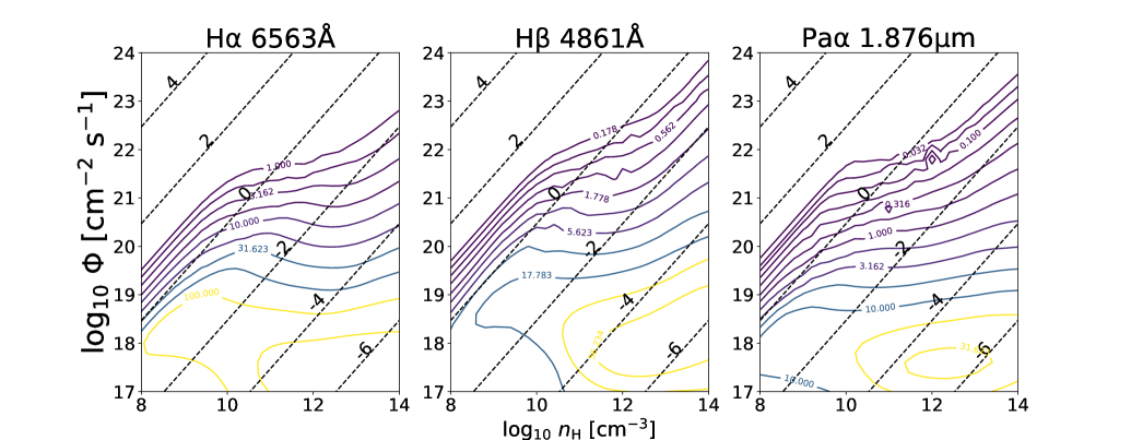
Figure 1: The equivalent width (EW) of H$\alpha$, H$\beta$, and Pa$\alpha$ emissions at different gas densities $n_{\rm H}$ and surface ionizing fluxes $\Phi_{\rm H}$ for a cloud with a hydrogen column density $N_{\rm H}=10^{23}\hbox{cm${}^{-2}$}$. The value of EW is marked for each contour. The dashed diagonal lines are photoionization parameters decreasing from the upper left ($\log_{10}U=4$) to the lower right ($\log_{10}U=-6$).

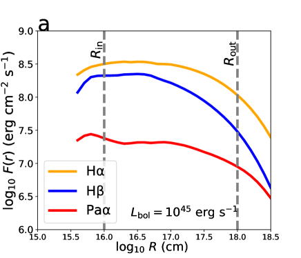
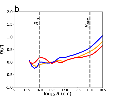
Figure 2: Panel a: radial emissivity function $F(r)$. Panel b: radial responsivity function $\eta(r)$ is calculated based on Equation (4). $R_{\rm in}$ and $R_{\rm out}$ are the inner and outer BLR boundaries in our calculation.

2.2 The definition of SA and RM size

The spectroastrometry size of BLR is actually the flux-weighted radius. As a result, the SA radius can be calculated as follows:

$$R_{\rm SA}=\frac{\iint_{R_{\rm in}}^{R_{\rm out}}r^{3}F(r)f(r)g(n)dndr}{\iint_{R_{\rm in}}^{R_{\rm out}}r^{2}F(r)f(r)g(n)dndr}.$$ (3)

The $F(r)$ curves of H$\alpha$, H$\beta$, Pa$\alpha$ are shown in Figure 2a.

The reverberation mapping (RM) size is actually the response-weighted radius. According to the previous works (Goad et al., 1993; Korista & Goad, 2004; Goad & Korista, 2014), the emission-line responsivity (in logarithmic space) to the changes in the incident hydrogen ionizing photon flux, can be written as:

$$\eta(r)=\frac{d\log_{10}F(r)}{d\log_{10}\Phi_{\rm H}}\propto-0.5\frac{d\log_{10}F(r)}{d\log_{10}r},{\rm since}\ \Phi_{\rm H}\propto r^{-2}.$$ (4)

The $\eta(r)$ of H$\alpha$, H$\beta$, Pa$\alpha$ are shown in Figure 2b. In linear space, the emission-line responsivity $dF(r)$/ $d\Phi_{\rm H}$=$[F(r)/\Phi_{\rm H}]\eta(r)\propto F(r)\eta(r)r^{2}$. As a result, the RM radius can be calculated as follows:

$$R_{\rm RM} = \frac{\iint_{R_{\rm in}}^{R_{\rm out}}r^{3}[dF(r)/d\Phi_{\rm H}]f(r)g(n)dndr}{\iint_{R_{\rm in}}^{R_{\rm out}}r^{2}[dF(r)/d\Phi_{\rm H}]f(r)g(n)dndr}$$ (5)

$$= \frac{\iint_{R_{\rm in}}^{R_{\rm out}}r^{5}F(r)\eta(r)f(r)g(n)dndr}{\iint_{R_{\rm in}}^{R_{\rm out}}r^{4}F(r)\eta(r)f(r)g(n)dndr}.$$ (6)

Figure 3: The radius ratio $K$ between of SA and RM size for several main hydrogen lines. Panels a, b, c: the combination of the same lines. Panels d, e, f: the combination of the different lines. The gray shadow is the region beyond the dust-limited outer BLR boundary $R_{\rm out}=10^{18}\ \rm cm$. We estimate the uncertainty of radius ratio $K=R_{\rm SA}/R_{\rm RM}$ under wide range of parameters: $-1.5<\Gamma<-0.5$, $\beta=-1$ and $10^{17.5}{\rm cm}<R_{\rm out}<10^{18}{\rm cm}$. The average and half-range of $K$ is marked in each panel. Surprisingly, not only the uncertainty of $K$ from the combination of the different lines are less than that from the combination of the same lines, but also the average values of $K$ from the combination of the different lines are closer to 1.

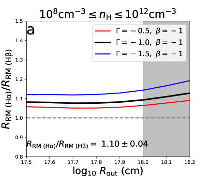
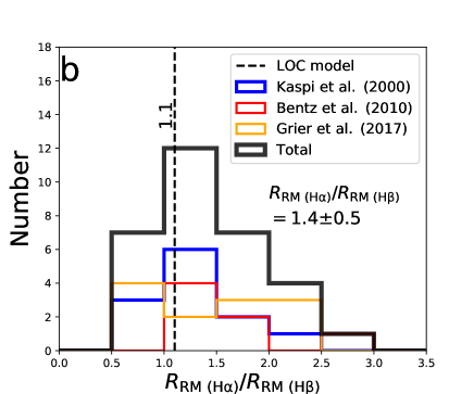
Figure 4: Panel a: the simulation radius ratio of H$\alpha$ to H$\beta$ of the RM measurements is $R_{\rm RM\ (H\alpha)}/R_{\rm RM\ (H\beta)}=1.10\pm 0.04$. All the symbols are the same as Figure 3. Panel b: the observational results of $R_{\rm RM\ (H\alpha)}/R_{\rm RM\ (H\beta)}$. The blue histogram represents measurements from Kaspi et al. (2000). The red histogram represents measurements from Bentz et al. (2010). The orange histogram represents measurements from Grier et al. (2017). The black histogram represents the sum of the above three samples. The mean and standard deviation of the distribution of observational $R_{\rm RM\ (H\alpha)}/R_{\rm RM\ (H\beta)}$ are $1.4\pm 0.5$. The vertical dashed line marks the mean value of simulated $R_{\rm RM\ (H\alpha)}/R_{\rm RM\ (H\beta)}$ based on LOC model. This simulation result is roughly consistent with the observational results.

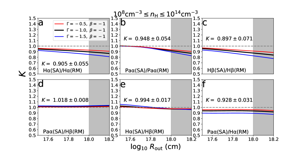
Figure 5: The radius ratio $K$ between of SA and RM size for several main hydrogen lines. All the parameters ranges and symbols are the same as Figure 3, except the gas density range. Here the density range is $10^{8}{\rm cm^{-3}}\leq n_{\rm H}\leq 10^{14}\rm cm^{-3}$.

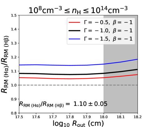
Figure 6: The simulation radius ratio of H$\alpha$ to H$\beta$ of the RM measurements is $R_{\rm RM\ (H\alpha)}/R_{\rm RM\ (H\beta)}=1.10\pm 0.05$. All the parameters ranges and symbols are the same as Figure 4, except the gas density range. Here the density range is $10^{8}{\rm cm^{-3}}\leq n_{\rm H}\leq 10^{14}\rm cm^{-3}$.

3 The deviation between SA and RM size

3.1 The simulation results

We adopt a radius ratio $K=R_{\rm SA}/R_{\rm RM}$ to describe the deviation between of SA and RM size. In this section, we will estimate the uncertainty of $K$ under the following parameter intervals which have been mentioned in the above section: $-1.5<\Gamma<-0.5$, $\beta=-1$, $10^{8}\hbox{cm${}^{-3}$}\leq n_{\rm H}\leq 10^{12}\hbox{cm${}^{-3}$}$, $N_{\rm H}=10^{23}\hbox{cm${}^{-2}$}$ and $10^{17.5}{\rm cm}<R_{\rm out}<10^{18}{\rm cm}$. We define the average and half-range of $K$ as: $\bar{K}=(K_{\rm max}+K_{\rm min})/2$ and $\Delta_{K}=(K_{\rm max}-K_{\rm min})/2$, where $K_{\rm max}$ and $K_{\rm min}$ are the maximum and minimum of $K$ under the parameter intervals, respectively. We firstly calculate the $K$ for the combination of the same lines. As shown in Figure 3a, 3b, 3c, the average and half-range of $K$ are $0.859\pm 0.063$, $0.879\pm 0.067$, $0.851\pm 0.083$ for the pairs of H$\alpha$(SA)/H$\alpha$(RM), Pa$\alpha$(SA)/Pa$\alpha$(RM), and H$\beta$(SA)/H$\beta$(RM), respectively. Surprisingly, all the averages of radius ratios $\bar{K}$ obtained from these same lines are much lower than 1 ($\sim 0.85-0.88$). For the combination of the different lines (Figure 3d, 3e, 3f), the average and half-range of $K$ are $0.974\pm 0.042$, $0.947\pm 0.028$, $0.894\pm 0.061$ for the pairs of Pa$\alpha$(SA)/H$\beta$(RM), H$\alpha$(SA)/H$\beta$(RM), and Pa$\alpha$(SA)/H$\alpha$(RM), respectively. Consequently, the corrected angular diameter distance $D^{\rm corr}_{\rm A}=R_{\rm SA}/\theta=K*R_{\rm RM}/\theta$=$K*D_{\rm A}$. According to the $z-D_{A}$ relation (Peacock, 1998), the corrected Hubble constant $H^{\rm corr}_{0}$=$H_{0}/K$, where $H_{0}$ is measured by the $D_{\rm A}$.

Interestingly, it clearly shows that not only the half-range of $K$ from the combination of the different lines are less than that from the combination of the same lines, but also the averages $\bar{K}$ from the combination of the different lines are closer to 1. As a result, the combination of the different lines are more suitable for the SARM project than the combination of the same lines. Among them, the $\bar{K}$ values from the Pa$\alpha$(SA)/H$\beta$(RM) and H$\alpha$(SA)/H$\beta$(RM) pairs are closest to 1 and have the smallest uncertainty.

At present, the interferometry technology has been achieved only in the infrared band K or longer wavelengths and for bright sources. For example, the GRAVITY of VLTI operates at the wavelengths range: 2.0–2.4 $\mu$m. For objects with a redshift $z<0.28$ the Pa$\alpha$ line is the only accessible strong broad line. Thus the Pa$\alpha$(SA)/H$\beta$(RM) pair is the best choice for the low redshift object in the SARM project. In the future, with a much larger collection area of telescopes and the advanced technology, it is possible to conduct interferometric observations for faint sources and to shorter wavelengths, enabling SARM for intermediate redshift quasars. In that case, a combination of H$\alpha$(SA)/H$\beta$(RM) would be fruitful.

3.2 Comparison between the simulation and observation for the RM measurements of H$\alpha$ and H$\beta$

In order to test the reliability of our simulation, we compare the simulation with the observation for the RM measurements of H$\alpha$ and H$\beta$. As shown in Figure 4a, the radius ratio of H$\alpha$ to H$\beta$ of the RM measurements is $R_{\rm RM\ (H\alpha)}/R_{\rm RM\ (H\beta)}=1.10\pm 0.04$. The definitions of the average and half-range of $R_{\rm RM\ (H\alpha)}/R_{\rm RM\ (H\beta)}$ are the same as for $K$. The observational results from Kaspi et al. (2000), Bentz et al. (2010) and Grier et al. (2017) are shown in Figure 4b. The black histogram in Figure 4b represents the sum of the above three papers. The mean and standard deviation of the distribution of observational $R_{\rm RM\ (H\alpha)}/R_{\rm RM\ (H\beta)}$ of the are $1.4\pm 0.5$. Both this simulation and observational results suggest that the H$\alpha$ region is slightly larger than that of H$\beta$. And our simulation result is roughly consistent with the observational results within a standard deviation. Therefore, our parameters selection of LOC model and simulation results are in a reasonable range.

3.3 Discussion

In general, the range of the number density of BLR gas can be considered as:$10^{8}\hbox{cm${}^{-3}$}\leq n_{\rm H}\leq 10^{12}\hbox{cm${}^{-3}$}$. However, as shown in Figure 1, the locations of EW peaks of H$\alpha$, H$\beta$ and Pa$\alpha$ lines are between $10^{12}\hbox{cm${}^{-3}$}\leq n_{\rm H}\leq 10^{14}\hbox{cm${}^{-3}$}$. Furthermore, the maximum value of BLR gas density can reach $10^{14}\hbox{cm${}^{-3}$}$ under the radiation pressure confinement (RPC, i.e., the equilibrium between the gas pressure and radiation pressure) model (Stern et al. 2014; Baskin et al. 2014). In view of this, it is necessary to check the simulation results when the maximum value of $n_{\rm H}$ reaches $10^{14}\hbox{cm${}^{-3}$}$. The radius ratios $K$ at the case of $10^{8}\hbox{cm${}^{-3}$}\leq n_{\rm H}\leq 10^{14}\hbox{cm${}^{-3}$}$ are shown in Figure 5. Similar to the case of $10^{8}\hbox{cm${}^{-3}$}\leq n_{\rm H}\leq 10^{12}\hbox{cm${}^{-3}$}$, not only the half-range of $K$ from the combination of the different lines (panels d, e, f) are less than that from the combination of the same lines (panels a, b, c), but also the averages of radius ratios $\bar{K}$ from the combination of the different lines are closer to 1. Similar to Figure 3, the $K$ values from the Pa$\alpha$(SA)/H$\beta$(RM) and H$\alpha$(SA)/H$\beta$(RM) pairs are also closest to 1 and have the smallest uncertainty. Furthermore, as shown in Figure 6, the radius ratio of H$\alpha$ to H$\beta$ of the RM measurements is $R_{\rm RM\ (H\alpha)}/R_{\rm RM\ (H\beta)}=1.10\pm 0.05$, which is similar to the case of $10^{8}\hbox{cm${}^{-3}$}\leq n_{\rm H}\leq 10^{12}\hbox{cm${}^{-3}$}$ (Figure 4). As a result, no matter the maximum value of the number density of BLR gas $10^{12}\hbox{cm${}^{-3}$}$ or $10^{14}\hbox{cm${}^{-3}$}$, the Pa$\alpha$(SA)/H$\beta$(RM) and H$\alpha$(SA)/H$\beta$(RM) pairs are always the best two choices for the SARM project.

As mentioned above, the RPC model (Baskin et al., 2014) is a more physically realistic BLR model which assumes that the gas pressure and radiation pressure are in equilibrium. In the RPC model, the cloud is no longer a uniform density slab, but has a density structure. In our next work, we will calculate the deviation between SA and RM size under the RPC model and make a comprehensive and detailed comparison with the LOC model.

4 Conclusion

The combination of interferometric and reverberation mapping for BLR of AGNs, can be used to measure the Hubble constant $H_{0}$. However, there may be a systematic deviation between these two different radii $R_{\rm SA}$ and $R_{\rm RM}$. In this work, we calculate this systematic deviation for three hydrogen lines H$\alpha$, H$\beta$, Pa$\alpha$ based on the LOC model of BLR. We estimate the half-range of radius ratio $K=R_{\rm SA}/R_{\rm RM}$ under sufficiently wide parameter ranges: $-1.5<\Gamma<-0.5$, $\beta=-1$, $10^{8}\hbox{cm${}^{-3}$}\leq n_{\rm H}\leq 10^{12}\hbox{cm${}^{-3}$}$, $N_{\rm H}=10^{23}\hbox{cm${}^{-2}$}$ and $10^{17.5}{\rm cm}<R_{\rm out}<10^{18}{\rm cm}$. Our main results can be summarized as follows:

• The ratios for the same line are systematically lower than unity by 10-15% for all hydrogen lines considered here (i.e.,H$\alpha$(SA)/H$\alpha$(RM), Pa$\alpha$(SA)/Pa$\alpha$(RM), and H$\beta$(SA)/H$\beta$(RM) ) and the scatter in these ratios are typically 0.06-0.08.

• The $K$ values from the Pa$\alpha$(SA)/H$\beta$(RM) and H$\alpha$(SA)/H$\beta$(RM) pairs are closest to 1 and have the smallest uncertainty.

Considering the current infrared interferometry technology, the Pa$\alpha$(SA)/H$\beta$(RM) pair is the best choice for the low redshift object in the SARM project. In the future, the H$\alpha$(SA)/H$\beta$(RM) pair could be used for the high redshift luminous quasars in the SARM project.

References

- Abuter et al. (2017) Abuter, R., Accardo, M., Amorim, A., et al. 2017, Astronomy & Astrophysics, 602, A94
- Bailey (1998) Bailey, J. 1998, Monthly Notices of the Royal Astronomical Society, 301, 161
- Baldwin et al. (1995) Baldwin, J., Ferland, G., Korista, K., & Verner, D. 1995, The Astrophysical Journal Letters, 455, L119
- Baskin et al. (2014) Baskin, A., Laor, A., & Stern, J. 2014, Monthly Notices of the Royal Astronomical Society, 438, 604
- Bentz et al. (2010) Bentz, M. C., Walsh, J. L., Barth, A. J., et al. 2010, The Astrophysical Journal, 716, 993
- Cackett et al. (2007) Cackett, E. M., Horne, K., & Winkler, H. 2007, Monthly Notices of the Royal Astronomical Society, 380, 669
- Collaboration et al. (2018) Collaboration, G., et al. 2018, Nature, 563, 657
- Collier et al. (1999) Collier, S., Horne, K., Wanders, I., & Peterson, B. M. 1999, Monthly Notices of the Royal Astronomical Society, 302, L24
- Czerny et al. (2013) Czerny, B., Hryniewicz, K., Maity, I., et al. 2013, Astronomy & Astrophysics, 556, A97
- Dunn et al. (2010) Dunn, J. P., Bautista, M., Arav, N., et al. 2010, The Astrophysical Journal, 709, 611
- Elvis & Karovska (2002) Elvis, M., & Karovska, M. 2002, The Astrophysical Journal Letters, 581, L67
- Ferland et al. (2017) Ferland, G., Chatzikos, M., Guzmán, F., et al. 2017, Revista mexicana de astronomía y astrofísica, 53
- Freedman (2017) Freedman, W. L. 2017, Nature Astronomy, 1, 1
- Goad et al. (1993) Goad, M., O’Brien, P., & Gondhalekar, P. 1993, Monthly Notices of the Royal Astronomical Society, 263, 149
- Goad & Korista (2014) Goad, M. R., & Korista, K. 2014, Monthly Notices of the Royal Astronomical Society, 444, 43
- Grier et al. (2017) Grier, C. J., Trump, J. R., Shen, Y., et al. 2017, The Astrophysical Journal, 851, 21
- Guo et al. (2020) Guo, H., Shen, Y., He, Z., et al. 2020, The Astrophysical Journal, 888, 58
- He et al. (2021) He, Z., Jiang, N., Wang, T., et al. 2021, The Astrophysical Journal Letters, 907, L29
- Hoenig & Kishimoto (2011) Hoenig, S. F., & Kishimoto, M. 2011, Astronomy & Astrophysics, 534, A121
- Hönig et al. (2017) Hönig, S., Watson, D., Kishimoto, M., et al. 2017, Monthly Notices of the Royal Astronomical Society, 464, 1693
- Hönig (2014) Hönig, S. F. 2014, The Astrophysical Journal Letters, 784, L4
- Kaspi et al. (2000) Kaspi, S., Smith, P. S., Netzer, H., et al. 2000, The Astrophysical Journal, 533, 631
- Kishimoto et al. (2007) Kishimoto, M., Hönig, S. F., Beckert, T., & Weigelt, G. 2007, Astronomy & Astrophysics, 476, 713
- Korista & Goad (2000) Korista, K. T., & Goad, M. R. 2000, The Astrophysical Journal, 536, 284
- Korista & Goad (2004) —. 2004, The Astrophysical Journal, 606, 749
- Koshida et al. (2014) Koshida, S., Minezaki, T., Yoshii, Y., et al. 2014, The Astrophysical Journal, 788, 159
- Landt et al. (2014) Landt, H., Ward, M. J., Elvis, M., & Karovska, M. 2014, Monthly Notices of the Royal Astronomical Society, 439, 1051
- Landt et al. (2019) Landt, H., Ward, M. J., Kynoch, D., et al. 2019, Monthly Notices of the Royal Astronomical Society, 489, 1572
- Nagao et al. (2006) Nagao, T., Marconi, A., & Maiolino, R. 2006, Astronomy & Astrophysics, 447, 157
- Nenkova et al. (2008) Nenkova, M., Sirocky, M. M., Nikutta, R., Ivezić, Ž., & Elitzur, M. 2008, The Astrophysical Journal, 685, 160
- Peacock (1998) Peacock, J. A. 1998, Cosmological Physics (Cambridge University Press), doi:10.1017/CBO9780511804533
- Planck Collaboration et al. (2020) Planck Collaboration, Aghanim, N., Akrami, Y., et al. 2020, A&A, 641, A6
- Riess et al. (2019) Riess, A. G., Casertano, S., Yuan, W., Macri, L. M., & Scolnic, D. 2019, The Astrophysical Journal, 876, 85
- Risaliti & Lusso (2019) Risaliti, G., & Lusso, E. 2019, Nature Astronomy, 3, 272
- Songsheng et al. (2021) Songsheng, Y.-Y., Li, Y.-R., Du, P., & Wang, J.-M. 2021, arXiv preprint arXiv:2103.00138
- Stern et al. (2014) Stern, J., Laor, A., & Baskin, A. 2014, Monthly Notices of the Royal Astronomical Society, 438, 901
- Sun et al. (2018) Sun, M., Xue, Y., Wang, J., Cai, Z., & Guo, H. 2018, The Astrophysical Journal, 866, 74
- Wang et al. (2020) Wang, J.-M., Songsheng, Y.-Y., Li, Y.-R., Du, P., & Zhang, Z.-X. 2020, NatAs, 4, 517
- Watson et al. (2011) Watson, D., Denney, K., Vestergaard, M., & Davis, T. M. 2011, The Astrophysical Journal Letters, 740, L49