Age of information distribution under dynamic service preemption

Abstract

Age of Information (AoI) has emerged as an important quality-of-service measure for applications that prioritize delivery of the freshest information, e.g., virtual or augmented reality over mobile devices and wireless sensor networks used in the control of cyber-physical systems. We derive the Laplace transform of the stationary AoI for the M/GI/1/2 system with a “dynamic” service preemption and pushout policy depending on the existing service time of the in-service message. Thus, our system generalizes both the static M/GI/1/2 queue-pushout system without service preemption and the M/GI/1/1 bufferless system with service preemption - two systems considered to provide very good AoI performance. Based on our analysis, for a service-time distribution that is a mixture of deterministic and exponential, we numerically show that the dynamic policy has lower mean AoI than that of these two static policies and also that of the well studied M/GI/1/1 blocking system.

1 Introduction

Consider a queueing system transmitting messages, particularly where the service-time distribution models access and transmission delays over a wireless channel. If $A(t)$ is the maximum arrival time of messages which are completely served before time $t$, then the quantity $\alpha(t)=t-A(t)$ is called “age of information” (AoI), see [12, 13] and references therein. The reason is simple: in several applications it is the freshness of information that is important rather than the correct transmission of all messages. Examples include virtual reality and online gaming on mobile devices, semi or fully autonomous vehicles, and wireless sensors of power systems and other “cyber physical” systems.

Mean AoI results for stationary systems are obtained in, e.g., [6, 4, 11, 9]. However, in such latency critical applications, bounds on the tail of the AoI distribution, e.g., [5, 8, 7], (not just its mean) need to be met. That is, for a threshold $\nu$ and tolerance $\varepsilon$ such applications require $\mathbb{P}(\alpha>\nu)<\varepsilon.$ (Note that, abusing notation, $\alpha$ will typicall stand for a random variable that is distributed according to $\alpha(t)$ for some, and hence all, $t$, when the process is stationary.)

Service preemption, last-in-first-out (LIFO) queueing, or queue push-out is often not practically feasible, but blocking/dropping of arriving messages typically is. The stationary distribution of AoI under blocking or push-out policies has been derived for different queueing models, including different buffer sizes and under preemptive or non-preemptive service, in [5, 8, 3, 7, 9]. Typically, renewal models of interarrival time and service time have been considered in prior work.

In particular, $\mathcal{P}_{1}$ (a system with at most one message and preemptive push-out service) has pathwise equal AoI as the infinite-buffer LIFO system with service preemption. Similarly, $\mathcal{P}_{2}$ (a system with at most two messages and non-preemptive service with push-out of the queued message) has pathwise smaller AoI than $\mathcal{B}_{2}$ (a blocking, non-preemptive system with at most two messages). When service times are deterministic, $\mathcal{P}_{2}$ was shown to have lower mean AoI than $\mathcal{P}_{1}$, though the converse is true when service times are exponential [11]. For deterministic service, $\mathcal{B}_{1}$ (non-preemptive service with at most one message in the system) has lower mean AoI than $\mathcal{P}_{2}$ for sufficiently large traffic loads under deterministic service. Ignoring practical constsraints on queueing policy, prior work has identified the policies $\mathcal{P}_{1}$, $\mathcal{P}_{2}$ or $\mathcal{B}_{1}$ as performing optimally by some AoI measure, particularly minimizing the mean AoI in steady-state. One can show $\mathcal{B}_{n}$ has pathwise smaller AoI than $\mathcal{B}_{n+1}$ for $n\geq 2$, however the same statement has not been proved for LIFO $\mathcal{P}_{n}$ policies, e.g., [9].

In this paper, we derive the AoI distribution for the stationary M/GI/1/2 system with a “dynamic” service preemption or queue-pushout policy depending on the amount of service received so far by the in-service message. As such, it is a causal queueing policy that generalizes both $\mathcal{P}_{1}$ and $\mathcal{P}_{2}$. The approach conditions on a well-known Markov-renewal embedding [2, 10] which can be employed to compute the AoI distribution for other such queueing systems [7], particularly LIFO systems with larger buffer sizes [9] and systems under the GI/M model (renewal arrivals and exponential service times).

We numerically show that for a particular serive-time distributions in the M/GI case that the dynamic policy has lower mean AoI than $\mathcal{P}_{1}$, $\mathcal{P}_{2}$ or $\mathcal{B}_{1}$. Our aim is to draw attention to an open problem: For a given queueing system model, what queuing and service policies minimize an AoI-based quality-of-service measure? Since for exponential service times, the memoryless property imples that the bufferless pushout system $\mathcal{P}_{1}$ has pathwise minimal AoI, we specifically exclude consideration of memoryless service times in the following.

This paper is organized as follows. In section 2, we define our queueing system and give some preliminary results. In section 3, we derive the AoI distribution of the stationary queuing system under consideration. Numerical comparisons with other systems based on mean AoI are made in Section 4. Finally, we summarize and discuss future work in Section 5.

2 System Definition and Preliminaries

There is a buffer consisting of two cells. Cell 1 is reserved for the message receiving service and cell 2 for the message waiting. If there is a message in cell $1$ at time $t$ we let $\mathfrak{u}(t)$ be the amount of service received by this message up to $t$; if the system is empty, we set $\mathfrak{u}(t)=0$. Fix $\theta\in[0,\infty]$. If a message arrives at time $t$ and $\mathfrak{u}(t)\leq\theta$ then the arriving message pushes-out the message in cell 1 and takes its place. Otherwise, if $\mathfrak{u}(t)>\theta$ then the arriving message occupies cell 2 (pushing out the message sitting there, if any). We call this system $\mathcal{P}_{2,\theta}$. Note that $\mathcal{P}_{2,0}$ and $\mathcal{P}_{2,\infty}$ make sense too and that the collection $\mathcal{P}_{2,\theta}$, $0\leq\theta\leq\infty$, is a “homotopy” between these two systems. In fact, in the terminology of [7, 8], $\mathcal{P}_{2,0}=\mathcal{P}_{2}$ and $\mathcal{P}_{2,\infty}=\mathcal{P}_{1}$. (In the latter system, cell 2 will never be occupied, so, effectively, it has buffer of size 1.)

Thus, a contiguous service interval that ends with a message departure is a sequence of preempted message-service periods followed by a completed/successful message-service period. Prior to the successful message-service period, there are no queued messages waiting for service. During the successful message-service period, any arriving messages obviously fail to preempt and, under queue pushout, the last such arriving message is queued and begins service once the successful message-service period ends.

We assume that the arrival process is Poisson with rate $\lambda>0$ and that messages have i.i.d. service times (independent of arrivals) distributed like a random variable $\sigma$ such that $\sigma>0$ a.s. with expectation $1/\mu<\infty$. We let $G$ be the distribution function of $\sigma$ and set $\hat{G}(s)=\mathbb{E}e^{-s\sigma}$. Under these assumptions, we will assume that the system $\mathcal{P}_{2,\theta}$ is in steady-state (taking into account that there is a unique such steady-state, the reasons for which are classical and will not be discussed here).

Let $S_{n}$ denote successful departure epochs. Let $K_{n}$ be the number of mesages in the system immediately after $S_{n}$. Given $K_{-1}=0$, consider Figure 1 at bottom.

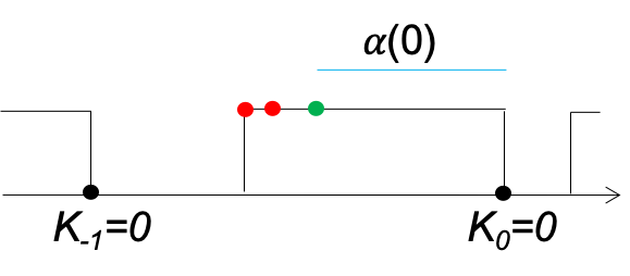
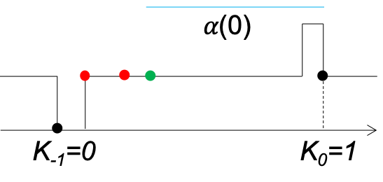
Figure 1: Number of messages in the system (black line) when $K_{-1}=0,K_{0}=0$ (top) and $K_{-1}=0,K_{0}=1$ (bottom). A black dot indicates a (successful) message departure. A green dot indicates an arrival of a message that will successfully depart. A red dot indicates an arrival of an unsuccessful message. If the fate of an arrival is not indicated in the figure, then it has no indicating dot. The length of the blue line is $\alpha(S_{0})$.

A message service period is successful with probability

$$1-q:=\mathbb{P}(\tau>\theta\wedge\sigma) =\int_{0}^{\infty}e^{-\lambda(\theta\wedge s)}dG(s)$$

$$=(1-G(\theta))e^{-\lambda\theta}+\int_{0}^{\theta}e^{-\lambda s}dG(s).$$

So, considering the successful service period which concludes at $S_{0}$:

$$\mathbb{P}(K_{0}=0|K_{-1}=0) =\mathbb{P}(\tau>\sigma~{}|~{}\tau>\theta\wedge\sigma)$$

$$=(1-q)^{-1}\hat{G}(\lambda)$$

$$=1-\mathbb{P}(K_{1}=1|K_{-1}=0).$$

Given $K_{-1}=1$, consider Figure 2.

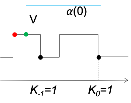
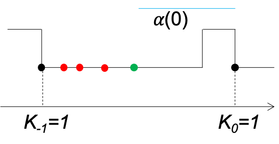
Figure 2: $K_{-1}=1,K_{0}=1$ cases.

.

Use the memoryless property of interarivals to similarly obtain

$$\mathbb{P}(K_{0}=0|K_{-1}=1) =(1-q)^{-1}\hat{G}(\lambda)$$

$$=1-\mathbb{P}(K_{0}=1|K_{-1}=1)$$

So, $K_{n}$ is an i.i.d. Bernoulli sequence with

$$p_{0} :=\mathbb{P}(K_{n}=0)=(1-q)^{-1}\hat{G}(\lambda)$$

$$=1-\mathbb{P}(K_{n}=1)=:1-p_{1}.$$

The queueing process over consecutive intervals $[S_{i-1},S_{i})$ and $[S_{i},S_{i+1})$ are conditionally independent given $K_{i}$. Thus, $\{S_{i},K_{i}\}_{i\in\mathbb{Z}}$ is Markov-renewal with renewal times $S_{i}$ and the queueing process is semi-Markov [2, 10]. In particular, $\alpha(S_{i})$ and $S_{i+1}-S_{i}$ are conditionally independent given $K_{i}$.

3 Stationary AoI Distribution

Proposition 1.

The Laplace transform of the stationary AoI distribution is

$$\mathbb{E}e^{-s\alpha(0)} =\frac{\sum_{i=0}^{1}\mathbb{E}^{0}(e^{-s\alpha(0)}|K_{0}=i)\Big{(}1-\mathbb{E}^{0}(e^{-s(S_{0}-S_{-1})}|K_{-1}=i)\Big{)}p_{i}}{s\mathbb{E}^{0}(S_{1}-S_{0})},$$ (1)

where $\mathbb{P}^{0}$ and $\mathbb{E}^{0}$ are respectively probability and expectation given $S_{0}=0$.

Proof.

The Palm inversion formula $\mathbb{E}e^{-s\alpha(0)}=$
${\mathbb{E}^{0}\int_{S_{0}}^{S_{1}}e^{-s\alpha(t)}dt}/{\mathbb{E}^{0}(S_{1}-S_{0})}$ has numerator

$$=\mathbb{E}^{0}\int_{S_{0}}^{S_{1}}e^{-s(\alpha(S_{0})+t-S_{0})}dt$$

$$=\mathbb{E}^{0}\int_{S_{0}}^{S_{1}}\sum_{i=0}^{1}(e^{-s\alpha(0)}|K_{0}=i)\mathbb{E}^{0}(e^{-s(t-S_{0})}|K_{0}=i)p_{i}dt$$

$$=\sum_{i=0}^{1}\mathbb{E}^{0}(e^{-s\alpha(0)}|K_{0}=i)\mathbb{E}^{0}\Bigg{(}\frac{1-e^{-s(S_{1}-S_{0})}}{s}\Bigg{|}K_{0}=i\Bigg{)}p_{i}$$

∎

To calculate the terms in (1) we need to follow the steps outlined in the lemmas below. Let $\hat{F}_{0}(s)=\hat{G}(s+\lambda)/\hat{G}(\lambda)$ and $\hat{J}(s)=\int_{0}^{\infty}e^{-sy}dJ(y)$ where $J(y)=1$ for $y\geq\theta$ and, for $0\leq y<\theta,$

$$dJ(y) =q^{-1}\lambda e^{-\lambda y}(1-G(y))dy$$

Lemma 1.

$$\mathbb{E}^{0}(e^{-s(S_{0}-S_{-1})}\mid K_{-1}=0,K_{0}=0)=\frac{\lambda}{\lambda+s}\cdot\frac{1-q}{1-q\hat{J}(s)}\hat{F}_{0}(s)$$ (2)

$$\mathbb{E}^{0}(e^{-s\alpha(S_{0})}\mid K_{-1}=0,K_{0}=0)=\hat{F}_{0}(s)$$ (3)

Proof.

See Figure 1 at top and consider the interval $[S_{-1},S_{0})$. Let $\tau_{-1}$ be first message arrival time in this interval minus $S_{-1}$, so that $\tau_{-1}\sim\exp(\lambda)$ by the memoryless property. Note that there is a geometric number $N$ of interarrival times each of which is smaller than both $\theta$ and the associated service time; $N=2$ in Figure 1. The probability of such unsuccessful service is

$$\mathbb{P}(\tau<\theta\wedge\sigma)=q.$$

So, $\mathbb{P}(N=k)=(1-q)q^{k}$ for $k=0,1,2,...$. Let $Y\stackrel{{\scriptstyle\text{\rm(d)}}}{{=}}(\tau|\tau<\theta\wedge\sigma)$ so that $\mathbb{P}(Y\leq y)=J(y)$. Finally, let $\tau_{0}\sim\exp(\lambda)$ be the duration between the arrival time (green dot) of the message that departs at $S_{0}$ and the next arrival time. The service time (from the green dot to $S_{0}$) $\sigma_{0}$ is independent of $\tau_{0}$. Considering the prior $N$ unsuccessful service completions, we are given that $\tau_{0}>\sigma_{0}$ or $\tau_{0}>\theta$. Given $K_{0}=0$, $\tau_{0}>\sigma_{0}$. Let $X_{0}\stackrel{{\scriptstyle\text{\rm(d)}}}{{=}}(\sigma_{0}|\tau_{0}>\sigma_{0})$ which has distibution

$$dF_{0}(x)=\hat{G}(\lambda)^{-1}e^{-\lambda x}dG(x),\quad x>0,$$

with $\mathbb{E}e^{-sX_{0}}=\hat{F}_{0}(s)$. So,

$$(S_{0}-S_{-1}\mid K_{-1}=0,K_{0}=0)\stackrel{{\scriptstyle\text{\rm(d)}}}{{=}}\tau_{-1}+\sum_{n=1}^{N}Y_{n}+X_{0},$$

a sum of independent terms with $Y_{n}\stackrel{{\scriptstyle\text{\rm(d)}}}{{=}}Y$. Also $\alpha(S_{0})\stackrel{{\scriptstyle\text{\rm(d)}}}{{=}}X_{0}$ in this case. ∎

Define

$$dF_{1}(x) =\frac{(e^{-\lambda\theta}-e^{-\lambda x})dG(x)}{\int_{\theta}^{\infty}(e^{-\lambda\theta}-e^{-\lambda z})dG(z)},\quad x>\theta$$

$$\hat{F}_{1}(s) =\int_{\theta}^{\infty}e^{-sx}dF_{1}(x).$$

Lemma 2.

$$\mathbb{E}^{0}(e^{-s(S_{0}-S_{-1})}\mid K_{-1}=0,K_{0}=1)=\frac{\lambda}{\lambda+s}\cdot\frac{1-q}{1-q\hat{J}(s)}\hat{F}_{1}(s)$$ (4)

$$\mathbb{E}^{0}(e^{-s\alpha(S_{0})}\mid K_{-1}=0,K_{0}=1)=\hat{F}_{1}(s).$$ (5)

Proof.

See Figure 1 at bottom. The difference between this and the previous case is that here $\sigma_{0}>\tau_{0}>\theta$. So, the distribution of $X_{1}\stackrel{{\scriptstyle\text{\rm(d)}}}{{=}}(\sigma_{0}\mid\sigma_{0}>\tau_{0}>\theta)$ is $dF_{1}(x)$, as defined above. ∎

Define

$$dH(v) =\frac{\lambda e^{-\lambda v}(1-G(v+\theta))dv}{\int_{\theta}^{\infty}(1-e^{-\lambda(x-\theta)})dG(x)},\quad v\geq 0,$$

$$\hat{H}(s) =\int_{0}^{\infty}e^{-sv}dH(v).$$

Lemma 3.

$$\mathbb{E}^{0}(e^{-s(S_{0}-S_{-1})}\mid K_{-1}=1,K_{0}=0)=\frac{1-q}{1-q\hat{J}(s)}\hat{F}_{0}(s)$$ (6)

$$\mathbb{E}^{0}(e^{-s\alpha(S_{0})}\mid K_{-1}=1,K_{0}=0)=q\hat{F}_{0}(s)+(1-q)\hat{H}(s)\times\eqref{expS_10}$$ (7)

Proof.

See Figure 3.

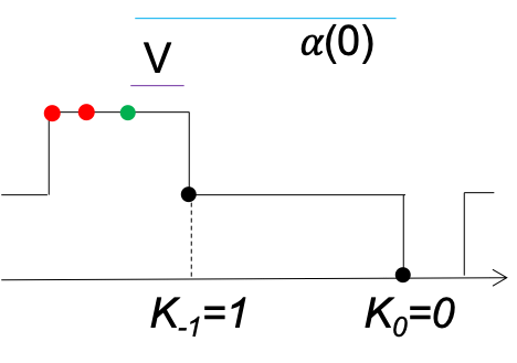
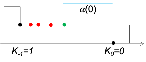
Figure 3: $K_{-1}=1,K_{0}=0$ cases.

.

For $\alpha(S_{0})$ there are two subcases depending of whether there are initial unsuccessful arrivals in the interval $[S_{-1},S_{0})$, i.e., whether $N>0$. When $N>0$ (Figure 3 bottom), this case is like when $K_{-1}=0,K_{0}=0$. Otherwise (Figure 3 top),

$$\alpha(S_{0})=V+S_{0}-S_{-1},$$

where $V$ is the duration between $S_{-1}$ the last arrival before $S_{-1}$ (green dot), and $V$ and $S_{0}-S_{1}$ are independent given $K_{-1}=1$. Starting from $S_{-1}$, look backward in time until the first Poisson point appears (green dot) and condition on the event that this occurs at least $\theta$ units of time before the service time ends. Thus, $V\stackrel{{\scriptstyle\text{\rm(d)}}}{{=}}(\tau|\tau<\sigma-\theta,\sigma>\theta)$ with distribution $H$. Also, $S_{0}-S_{-1}$ is distributed as for the case where $K_{-1}=0,K_{0}=0$ except the first interarrival time is absent. ∎

Lemma 4.

$$\mathbb{E}^{0}(e^{-s(S_{0}-S_{-1})}\mid K_{-1}=1,K_{0}=1)=\frac{1-q}{1-q\hat{J}(s)}\hat{F}_{1}(s)$$ (8)

$$\mathbb{E}^{0}(e^{-s\alpha(S_{0})}\mid K_{-1}=1,K_{0}=1)=q\hat{F}_{1}(s)+(1-q)\hat{H}(s)\times\eqref{expS_11}$$ (9)

Proof.

See Figure 2. For $S_{0}-S_{-1}$, this case is a combination of the previous two cases, and for $\alpha(S_{0})$ follow the previous case except use (5) instead of (3). ∎

The final stage: The formulas obtained in the lemmas above must now be substituted into (1) as follows:

$$\mathbb{E}^{0}(e^{-s(S_{0}-S_{-1})}|K_{-1}=0)=\eqref{expS_01}\times p_{1}+\eqref{expS_00}\times p_{0}$$ (10)

$$\mathbb{E}^{0}(e^{-s(S_{0}-S_{-1})}|K_{-1}=1)=\eqref{expS_11}\times p_{1}+\eqref{expS_10}\times p_{0}.$$ (11)

So,

$$\mathbb{E}^{0}(S_{1}-S_{0})=-\frac{d}{ds}\mathbb{E}^{0}e^{-s(S_{0}-S_{-1})}\Bigg{|}_{s=0}=-\frac{d}{ds}(p_{1}\times\eqref{ES_1}+p_{0}\times\eqref{ES_0})\Bigg{|}_{s=0}.$$

Moreover,

$$\mathbb{E}^{0}(e^{-s\alpha(0)}|K_{0}=0) =p_{0}\times\eqref{expA_00}+p_{1}\times\eqref{expA_10}$$

$$\mathbb{E}^{0}(e^{-s\alpha(0)}|K_{0}=1) =p_{0}\times\eqref{expA_01}+p_{1}\times\eqref{expA_11}.$$

4 Numerical Results for Stationary Mean AoI, $\mathbb{E}\alpha(0)$

The stationary mean AoI can be obtained from (1) and numerically minimized over $\theta$ for a given set of model parameters for an arbitrary service-time distribution $G$. For example, for exponential service times, $dG(x)=\mu e^{-\mu x}dx$, and $\theta=\infty$ ($\mathcal{P}_{1}$) achieves minimal $\mathbb{E}\alpha(0)=\mu^{-1}+\lambda^{-1}$ [11, 5, 8]. For another example, for constant service time $dG(x)=\delta_{1/\mu}(x)dx$, the $\mathcal{P}_{2}$ system (i.e., when $\theta=0$) has

$$\mathbb{E}\alpha(0)\;=\;\frac{1}{\mu}\left(\left(1-e^{-\rho}\right)\left(1+\frac{1}{\rho}\right)+\frac{1}{\rho^{2}+\rho e^{-\rho}}\,\left(e^{-\rho}+\rho e^{-\rho}+\frac{1}{2}\rho^{2}\right)\right);$$

which is generally smaller than $\mathcal{P}_{1}$ (and also smaller than $\mathcal{B}_{1}$ for sufficiently small traffic loads [5, 8, 7]).

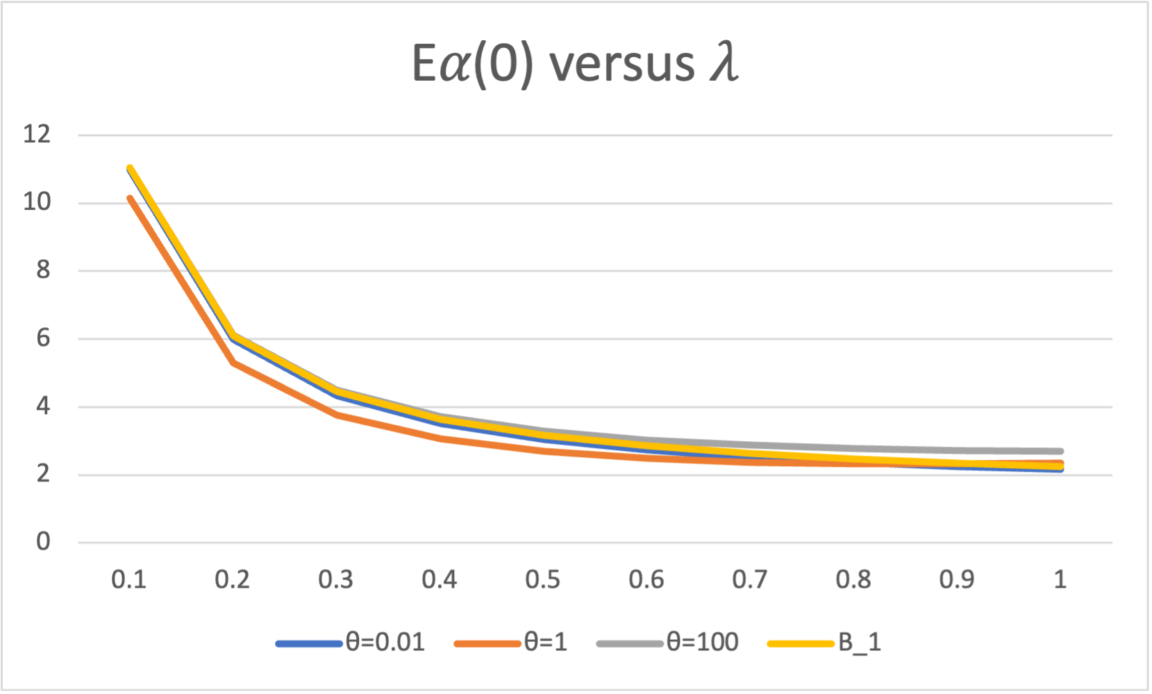
Figure 4: $\mathbb{E}\alpha(0)$ for service-time distribution which is a mixture of deterministic and exponential with mean $\mu^{-1}=1$.

Now consider the mixture service-time distribution defined by $dG(x)=\frac{1}{2}\delta_{1}(x)dx+\frac{1}{2}e^{-x}dx$ for $x>0$, and so $\mu=1$. From Figure 4, which was obtained numerically using (1), we see that in some cases $\mathbb{E}\alpha(0)$ is not minimized at either $\theta=0$ or $\theta=\infty$. That is, in some cases (specifically, traffic loads $\leq 0.8$), the $\mathcal{P}_{2,\theta}$ policy for a finite $\theta>0$ ($\theta=1$ in Figure 4) has lower mean AoI than $\mathcal{P}_{1}$, $\mathcal{P}_{2}$ and $\mathcal{B}_{1}$.

5 Summary and Future Work

In this paper, we analyzed the Age of Information performance of the $\mathcal{P}_{2,\theta}$ queueing policy in steady state under the M/GI model (Poisson message arrivals and i.i.d. service times). $\mathcal{P}_{2,\theta}$ can hold at most two messages in the system and dynamically employs either queue push-out or service preemption depending on whether the system is full and on the service-time-so-far of the in-service message. We numerically demonstrated that it has lower mean AoI than previously studied $\mathcal{P}_{2}$, $\mathcal{P}_{1}$ and $\mathcal{B}_{1}$ policies for a service time distribution that is a mixture of deterministic and exponential.

Using the Markov embedding approach we employed, one can also analyze variations of the $\mathcal{P}_{2,\theta}$ policy in the same way. For example, consider the policy where a message arriving at time $t$ does not preempt the in-service message (but joins the queue in cell 2) if $0<\mathfrak{u}(t)<\theta$, otherwise the message captures the server.

In future work, we will consider the problem of determining a queuing and service policy that is optimal with respect to an AoI based quality-of-service metric when interarrival time and service time models are specified. In practice, this question may subject to technological constraints which may preclude use of, e.g., service preemption and/or queue push-out. Also, we will consider the problem of deriving the AoI distribution for specific interarrival time and service time models of the non-renewal type.

References

- [1] A.M. Bedewy, Y. Sun, and N.B. Shroff. Minimizing the age of information through queues. IEEE Transactions on Information Theory, 65(8), Aug. 2019.
- [2] E. Çinlar. Introduction to Stochastic Processes. Dover, 1975.
- [3] J. P. Champati, H. Al-Zubaidy, and J. Gross. On the Distribution of AoI for the GI/GI/1/1 and GI/GI/1/2* Systems: Exact Expressions and Bounds. In Proc. IEEE INFOCOM, 2019.
- [4] M. Costa, M. Codreanu, and A. Ephremides. On the Age of Information in Status Update Systems With Packet Management. IEEE Transactions on Information Theory, 62(4), April 2016.
- [5] Y. Inoue, H. Masuyama, T. Takine, and T. Tanaka. A General Formula for the Stationary Distribution of the Age of Information and Its Application to Single-Server Queues. IEEE Transactions on Information Theory, 65(12), Dec. 2019.
- [6] S. Kaul, R.D. Yates, and M. Gruteser. Real-time status: How often should one update? In Proc. IEEE INFOCOM, 2012.
- [7] G. Kesidis, T. Konstantopoulos, and M.A. Zazanis. Age of information without service preemption. http://arxiv.org/abs/2104.08050, Apr. 2021.
- [8] G. Kesidis, T. Konstantopoulos, and M.A. Zazanis. The new age of information: a tool for evaluating the freshness of information in bufferless processing systems. Queueing Systems: Theory and Applications, 95(3):203–250, Aug. 2020; http://arxiv.org/abs/1904.05924; https://arxiv.org/abs/1808.00443.
- [9] G. Kesidis, T. Konstantopoulos, and M.A. Zazanis. Age of Information for a LIFO system with Poisson Arrivals and Small Buffer Size. http://arxiv.org/abs/2106.08473, May 2021.
- [10] L. Kleinrock. Queueing Systems Volume I: Theory. Wiley, 1975.
- [11] A. Kosta, N. Pappas, and V. Angelakis. Age of information: A new concept, metric, and tool. Foundations and Trends in Networking, 12(3):162–259, 2017.
- [12] Y. Sun, I. Kadota, R. Talak, and E. Modiano. Age of Information: A New Metric for Information Freshness. Synthesis Lectures on Communication Networks, Dec. 2019.
- [13] R.D. Yates, Y. Sun, D.R. Brown, S.K. Kaul, E. Modiano, and S. Ulukus. Age of Information: An Introduction and Survey. IEEE Journal on Selected Areas in Communications, 39(5), May 2021.