Convexification-based globally convergent numerical method for a 1D coefficient inverse problem with experimental data

Michael V. Klibanov Department of Mathematics and Statistics, University of North Carolina at Charlotte, Charlotte, NC 28223, USA, mklibanv@uncc.edu (corresponding author), tle55@uncc.edu, loc.nguyen@uncc.edu    Thuy T. Le11footnotemark: 1    Loc H. Nguyen11footnotemark: 1    Anders Sullivan US Army Research Laboratory, 2800 Powder Mill Road, Adelphi, MD 20783-1197, USA, (anders.j.sullivan.civ@mail.mil, lam.h.nguyen2civ@mail.mil)    Lam Nguyen22footnotemark: 2
Abstract

To compute the spatially distributed dielectric constant from the backscattering data, we study a coefficient inverse problem for a 1D hyperbolic equation. To solve the inverse problem, we establish a new version of Carleman estimate and then employ this estimate to construct a cost functional which is strictly convex on a convex bounded set with an arbitrary diameter in a Hilbert space. The strict convexity property is rigorously proved. This result is called the convexification theorem and is considered as the central analytical result of this paper. Minimizing this convex functional by the gradient descent method, we obtain the desired numerical solution to the coefficient inverse problems. We prove that the gradient descent method generates a sequence converging to the minimizer and we also establish a theorem confirming that the minimizer converges to the true solution as the noise in the measured data and the regularization parameter tend to zero. Unlike the methods that are based on optimization, our convexification method converges globally in the sense that it delivers a good approximation of the exact solution without requiring any initial guess. Results of numerical studies of both computationally simulated and experimental data are presented.

Key words: experimental data, convexification, 1D hyperbolic equation, coefficient inverse problem, globally convergent numerical method, Carleman estimate, numerical results

AMS subject classification: 35R30, 78A46

1 Introduction

We develop a new version of the convexification method to numerically solve a highly nonlinear and severely ill-posed inverse problem for a 1D hyperbolic equation. Applications of this technique are in detection and identification of explosives, see some details in Section 7. This paper belongs to a series of works that establish a variety of versions of the convexification method to solve nonlinear inverse problems for many partial differential equations [15, 16, 24, 25, 27, 28, 30, 31, 32, 33, 52]. The key point of the convexification method for each inverse problem in those publications is to use a suitable weight function to construct a globally strictly convex weighted Tikhonov-like functional. The weight is the Carleman Weight Function (CWF), i.e. the function which is involved as the weight in the Carleman estimate for the corresponding Partial Differential Operator. The unique minimizer of such a functional directly yields the desired numerical solution of that nonlinear inverse problem. The above mentioned global strict convexity guarantees that we can solve that nonlinear inverse problem without any advanced knowledge of the true solutions. Therefore, we say that our convexification method is globally convergent. By “globally convergent”, we mean:

  1. 1.

    There exists a theorem rigorously confirming that our method delivers at least one point in a sufficiently small neighborhood of the exact solution without requiring a good initial guess of the true solution;

  2. 2.

    This theorem is verified numerically.

In this paper, item 1 is reached by establishing a new Carleman estimate and applying it to prove a new version of the convexification theorem. Item 2 is reached for both computationally simulated data and experimental data.

We also refer here to some recent publications of another research group [2, 3, 6] and the publication [43] by members of our group. These papers work on two different versions of the convexification. CWFs still play a crucial role in both versions. We now describe the main difference between our above cited works and ones of this group. Papers [2, 3, 6, 43] work for the case when at least one of initial conditions is not vanishing. Unlike this, we consider in almost all above cited publications the case when the initial condition in a hyperbolic equation is the Dirac $\delta-$function and similar conditions for CIPs for the Helmholtz equation. In this regard, the only exception is the publication [32], which also works for the case when a sort of an initial condition is not vanishing.

Let $n(x)$ be the refractive index and let $c(x)=n^{2}(x)$ for all $x\in\mathbb{R}$ be the spatially distributed dielectric constant. If we scale the speed of light traveling in the air or vacuum to be $1$, then $1/\sqrt{c(x)}$ is the speed of light in the medium. Let $\epsilon$ and $M$ be two fixed numbers with $0<\epsilon\ll 1<M<\infty$. Assume that the spatially distributed dielectric constant $c$ belongs to $C^{3}(\mathbb{R})$ and that

$$c(x)=\left\{\begin{array}[]{ll}\in[\underline{c},\overline{c}]&\mbox{if }x\in[\epsilon,M],\\ 1&\mbox{otherwise}\end{array}\right.$$ (1.1)

for some known constants $0<\underline{c}<\overline{c}<\infty.$ The smoothness condition $c\in C^{3}(\mathbb{R})$ is imposed only for the theoretical part while it can be relaxed in the numerical study. Let $u=u(x,t)$, $(x,t)\in\mathbb{R}\times[0,\infty)$, be the solution to the following initial value problem

$$\left\{\begin{array}[]{rcll}c(x)u_{tt}(x,t)&=&u_{xx}(x,t)&(x,t)\in\mathbb{R}\times(0,\infty),\\ u(x,0)&=&0&x\in\mathbb{R},\\ u_{t}(x,0)&=&\delta_{0}(x)&x\in\mathbb{R},\end{array}\right.$$ (1.2)

where $\delta_{0}$ is the Dirac function with its support $\left\{0\right\}$. The problem of our interest is formulated as follows.

Problem 1.1 (Coefficient inverse problem).

Let $T>0$ be the length of the time interval. Measuring the functions $g_{0}(t)$ and $g_{1}(t),$

$$g_{0}(t)=u(\epsilon,t)\quad\mbox{and }\quad g_{1}(t)=u_{x}(\epsilon,t)$$ (1.3)

for $t\in[0,T+\epsilon],$ determine the function $c(x)$ for all $x\in[\epsilon,M].$

We refer the reader to [9, 14, 37, 46] for some uniqueness and stability results for coefficient inverse problems that are similar to Problem 1.1 to identify $c,$ given the Dirichlet-to-Neumann map data. The uniqueness and stability results for Problem 1.1 follow from [50] (chapter 2) as well as directly from our computational method in this paper. In [11] the Gelfand-Levitan method [8] was numerically implemented for a similar CIP. Next, this method was extended to the 2D case [11, 12].

Problem 1.1 arises from the following experiment. Let an emitter sends an electric wave into the inspected area, in which the target we want to identify is hidden. Then, we measure the back scattering wave using a detector located near the emitter. An example of this device is the Forward Looking Radar built by the US Army Research Laboratory (ARL) [49]. This radar device is placed on the top of a moving vehicle during the data collecting process, see [49] for more details. Since the given data has one dimension for each target, reconstructing $d-$dimensional function with $d>1$ is impossible. Thus, we have no choice but to model the wave propagation by a 1D hyperbolic equation. This 1D model was verified numerically multiple times in the past in the sense that it can be used to successfully compute the dielectric constants of explosive-like targets from experimental data provided by ARL, see [13, 29, 30, 35, 38, 53].

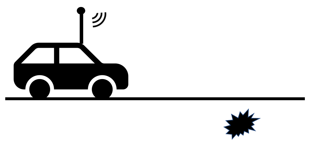
By solving Problem 1.1, we obtain the spatially distributed dielectric constant. This computed dielectric constant provides the location and some information about the constituent material of the target. This problem has applications in detecting antipersonnel explosive devices. The latter is one of important Army’s interests. In this experiment, only $g_{0}$ is measured while the data $g_{1}$ is missing. However, in Section 7, we explain how to approximate the missing function $g_{1}$. The schematic diagram of the data collection is displayed on Figure 1.We have also discovered recently that Problem 1.1 plays the key role in the nonlinear synthetic-aperture radar (SAR) imaging, including SAR experimental data [17, 26].

Refer to caption
(a) The target is placed in the air
Refer to caption
(b) The target is buried under the ground
Figure 1: The schematic for the data generating and collecting device. A device, called radar, emits an acoustic source and then collect the time-dependent backscattering wave. In the physical experiment, we consider two cases: (a) the target is placed in the air and (b) the target is buried a few centimeters under the ground.

Natural approaches for solutions of nonlinear inverse problems, that are widely used in the scientific community, are based on the least-squares optimization. However, the use of optimization-based methods is limited to the case when a good initial guess for the true solution of Problem 1.1 is known. However, it is rarely available in the reality. This requirement is due to the fact that the those least-squares functionals are non convex and typically have multiple local minima and ravines, see, e.g. [51, Figure 1] for a convincing example of this well-known challenge. Hence, the least-squares optimization method is not applicable to solve Problem 1.1. Another approach to solve Problem 1.1 is the use of the Born approximation or Born series. This approach is effective if the true dielectric constant is a sufficiently small perturbation of a known background function. Hence, the methods based on Born approximation or/and Born series work for the case when the size of the target is small and the contrast $c_{\mathrm{target}}/c_{\mathrm{bckgr}}\ll 1$ where $c_{\mathrm{target}}$ is the dielectric constant of the target and $c_{\mathrm{bckgr}}$ is the dielectric constant of the background (or the environment around the target). For example, it was demonstrated numerically on [17] that the Born approximation is not capable to deliver accurate values of dielectric constants of targets for SAR-like data in the case of high target/background contrasts.

To overcome these limitations, Klibanov and Ioussoupova introduced the convexification method [25]. Since then, it has been intensively applied to solve nonlinear coefficient inverse problems [1, 15, 16, 19, 20, 23, 27, 28, 31, 33, 52, 53]. The reconstructions due to the convexification are successful even for the challenging case of experimental data [15, 28, 53]. The main idea of the convexification is to employ CWFs and Carleman estimates to convexify the least-squares functional. In other words, when we employ a suitable CWF in the mismatch functional, the resulting functional is strictly convex on a convex bounded set of an arbitrary diameter in an appropriate Hilbert space. The minimizer of this strictly convex functional, which can be found without an initial guess, is an approximation of the desired solution. Hence, we claim and then prove that our numerical method is globally convergent, see the first paragraph of this section for the definition of globally convergent.

The original idea of applying Carleman estimates to coefficient inverse problems was first published in [7] back in 1981 by Bukhgeim and Klibanov to prove uniqueness theorems for a wide class of coefficient inverse problems. Some follow up publications can be found in, e.g. [10, 18, 36, 43, 47, 48, 55]. Surveys on the Bukhgeim-Klibanov method can be found in [21, 56], also, see section 1.10 of the book [4, Chapter 1]. It was discovered later in [25] that the idea of [7] can be used to develop globally convergent numerical methods for coefficient inverse problems using the convexification.

The inverse problem in this paper, Problem 1.1, is identical with the inverse problem in [52, 53]. The convexification method in [52, 53] is effective but there are some rooms to improve. The method of [52, 53] has two stages. On stage 1, the authors used the well-known change of variables as in [50, Chapter 2, §7] to reduce the original inverse problem to the inverse problem of computing the potential of a 1D hyperbolic equation. This resulting inverse problem to compute the potential can be solved using one of two versions of the convexificaton method of either [52] or [53]. On stage 2, the authors computed the dielectric constant from the knowledge of the reconstructed potential of stage 1. This second stage is a quite complicated one, due to that change of variables, and caused many difficulties in its numerical implementation. This motivates us to propose a different version of the convexification method in this paper. In this paper, we solve Problem 1.1 directly, i.e. without the change of variable of [50, Chapter 2, §7]. By this, the numerical implementation is significantly simplified.

The key points that guarantee the success of our method involve:

  1. 1.

    The derivation of a nonlinear and non local partial differential equation without the presence of the unknown coefficient.

  2. 2.

    Two new Carleman estimates for this equation.

  3. 3.

    A new version of the convexification method to solve the above equation.

  4. 4.

    The theorem ensuring the global strict convexity of the cost functional constructed by the convexification method of item 3.

  5. 5.

    The theorem, which guarantees the global convergence of the gradient descent method of the minimization of the strictly convex functional resulting from the convexification method.

Since Problem 1.1 is a coefficient inverse problem for a 1D hyperbolic equation, we mention here works [33, 34] in which the authors solved 3D versions of Problem 1.1. In [33] a coefficient inverse problem for the 3D analog of equation (1.2) with a single location of the source was solved numerically via a version of the convexification method. In [34] a coefficient inverse problem of the 3D analog of equation (1.2) with the point source running along a straight line was solved via the linear integral equation invented by M.M. Lavrent’ev in 1964 [41]; also, see formula (7.18) of the book [42] for this equation. A new numerical method for the solution of the Lavrent’ev equation was proposed in [34].

This paper is organized as follows. In Section 2, we derive an important equation. Solution of this equation can be directly used to compute the desired dielectric constant. In Section 3, we prove a new Carleman estimate. This estimate is an important generalization of the one in [52]. In Section 5, we prove the convexification theorem. Also in Section 5, we prove the global convergence of the gradient descent method of the minimization of the globally strictly convex cost functional constructed by the convexification method. In Section 6, we present the numerical results obtained for computationally simulated data. In Section 7, we present the numerical results obtained from experimental data. Concluding remarks are made in Section 8.

2 A Partial Differential Equation in Which the Unknown Coefficient is Not Present

For each $x\in\mathbb{R}$, define

$$\tau(x)=\int_{0}^{x}\sqrt{c(s)}ds.$$ (2.1)

The function $\tau(x)$ is the travel time. This is the time the wave needs to propagate from the source position $\left\{x=0\right\}$ to the point $x$, see [50, Chapter 2, §7]. It is well-known that $\tau$ satisfies the eikonal equation

$$|\tau^{\prime}(x)|^{2}=c(x),\quad\mbox{for all }x>\epsilon.$$ (2.2)

Since $c(x)=1$ for all $x<\epsilon$, see condition (1.1), then

$$\tau(x)=x,\quad\mbox{for all }x\leq\epsilon.$$ (2.3)

In particular,

$$\tau(\epsilon)=\epsilon.$$ (2.4)

The following lemma is important for derivation of the numerical method in this paper.

Lemma 2.1.

The function $u(x,t)$ has the form

$$u(x,t)=\frac{H(t-|\tau(x)|)}{2c^{1/4}(x)}+\widehat{u}(x,t),\quad(x,t)\in\mathbb{R}\times(0,\infty)$$ (2.5)

where $\widehat{u}$ is a function in $C^{2}(t\geq\tau(x))$ and $\widehat{u}(x,\tau(x))=0$. As a result,

$$\lim_{t\to\tau(x)^{+}}u(x,t)=\frac{1}{2c^{1/4}(x)},\quad\mbox{for all }x>\epsilon.$$ (2.6)

Proof. By (2.1) $\tau\left(x\right)$ is an increasing function and has an inverse. Recall the well-known change of variable, see formulas (8) and (9) in [53],

$\displaystyle v(x,t)$ $\displaystyle=\displaystyle u(\tau^{-1}(x),t)c^{1/4}(\tau^{-1}(x)),$ $\displaystyle\mbox{for all }x\in\mathbb{R},t\in(0,\infty),$ (2.7)
$\displaystyle\ S(x)$ $\displaystyle=\displaystyle c^{-1/4}(\tau^{-1}(x)),$ $\displaystyle\mbox{for all }x\in\mathbb{R},$ (2.8)
$\displaystyle r(x)$ $\displaystyle=\displaystyle\frac{S^{\prime\prime}(x)}{S(x)}-2\Big{[}\frac{S^{\prime}(x)}{S(x)}\Big{]}^{2},$ $\displaystyle\mbox{for all }x\in\mathbb{R}.$ (2.9)

By a straightforward computation, we deduce from (1.2), (2.7), (2.8) and (2.9) that

$$\left\{\begin{array}[]{rcll}v_{tt}(x,t)&=&v_{xx}(x,t)+r(x)v(x,t)&x\in\mathbb{R},t\in(0,\infty),\\ v(x,0)&=&0&x\in\mathbb{R},\\ v_{t}(x,0)&=&\delta_{0}(x)&x\in\mathbb{R}.\end{array}\right.$$

Hence, $v$ has the form, see [50, Chapter 2, §3],

$$v(x,t)=\frac{H(t-|x|)}{2}+\frac{1}{2}\int_{(x-t)/2}^{(x+t)/2}r(\xi)\Big{(}\int_{|\xi|}^{t-|x-\xi|}v(\xi,\tau)d\tau\Big{)}d\xi.$$ (2.10)

Using (2.7) and (2.10, we obtain for all $x\in\mathbb{R}$, $t\in(0,\infty)$

$$u(x,t)c^{1/4}(x)=v(\tau(x),t)=\frac{H(t-|\tau(x)|)}{2}+\frac{1}{2}\int_{(\tau(x)-t)/2}^{(\tau(x)+t)/2}r(\xi)\Big{(}\int_{|\xi|}^{t-|\tau(x)-\xi|}v(\xi,\tau)d\tau\Big{)}d\xi.$$

We obtain (2.5). Formula (2.6) is a direct consequence of (2.5).    

We also need Lemma 2.2 below, which is a direct consequence of one of results of [52, Lemma 2.2]. Using this lemma, we establish a boundary condition at $x=M$ where we cannot measure any information of the function $u$.

Lemma 2.2. (Absorbing boundary condition) Assume that $M>\max\{c(x):x\in R\}$. Then

$$u_{x}(M,t)+u_{t}(M,t)=0,\quad\mbox{for all }t>0$$ (2.11)

and

$$u_{x}(x,t)-u_{t}(x,t)=0,\quad\mbox{for all }x<0,t>0.$$ (2.12)

Let $\Omega_{T}=(\epsilon,M)\times(0,T).$ Introduce the change of variables,

$$q(x,t)=u(x,t+\tau(x)),\quad\mbox{for all }(x,t)\in\Omega_{T}$$ (2.13)

where $u$ is the solution of (1.2). We derive a partial differential equation for the function $q$, in which the function $c$ is not present. The first step is to show that $q(x,0)>0$ for all $x>\epsilon$. In fact, using (2.13) with $t=0$ and (2.6) with $t=\tau(x)^{+}=\tau(x)$, we obtain

$$q(x,0)=u(x,\tau(x))=\frac{1}{2c^{1/4}(x)}\geq\underline{q}:=\frac{1}{2\overline{c}^{1/4}}>0,\quad\mbox{for all }x>\epsilon$$ (2.14)

where $\overline{c}$ is a known upper bound of the function $c$, see (1.1). The estimate (2.14) is important because we will see later in this section that $q(x,0)$ is the denominator of some components for the desired differential equation that governs the function $q$. We next differentiate (2.13) with respect to $x$ to obtain

$$q_{x}(x,t)=u_{x}(x,t+\tau(x))+u_{t}(x,t+\tau(x))\tau^{\prime}(x)$$ (2.15)

for all $x>\epsilon$, $t>0$. Thus, for all $x>\epsilon$, $t>0$, we obtain

$$q_{xt}(x,t)=u_{xt}(x,t+\tau(x))+u_{tt}(x,t+\tau(x))\tau^{\prime}(x)$$ (2.16)

and

$$q_{xx}(x,t)=u_{xx}(x,t+\tau(x))+2u_{xt}(x,t+\tau(x))\tau^{\prime}(x)+u_{tt}(x,t+\tau(x))|\tau^{\prime 2}\\ +u_{t}(x,t+\tau(x))\tau^{\prime\prime}(x).$$ (2.17)

It follows from the governing equation (1.2), the eikonal equation (2.2), (2.16), and (2.17) that

$\displaystyle q_{xx}(x,t)$ $\displaystyle=2u_{xt}(x,t+\tau(x))\tau^{\prime}(x)+2u_{tt}(x,t+\tau(x))|\tau^{\prime 2}+u_{t}(x,t+\tau(x))\tau^{\prime\prime}(x)$
$\displaystyle=2q_{xt}(x,t)\tau^{\prime}(x)+u_{t}(x,t+\tau(x))\tau^{\prime\prime}(x)$
$\displaystyle=2q_{xt}(x,t)\tau^{\prime}(x)+q_{t}(x,t)\tau^{\prime\prime}(x)$ (2.18)

for all $x>\epsilon,t>0.$ We next eliminate $\tau$ from (2.18). Using (2.1) and (2.14), we have

$$\tau^{\prime}(\mathbf{x})=\sqrt{c(x)}=\frac{1}{4q^{2}(x,0)}.$$ (2.19)

Therefore, for all $x>\epsilon$

$$\tau^{\prime\prime}(\mathbf{x})=-\frac{q_{x}(x,0)}{2q^{3}(x,0)}.$$ (2.20)

Combining (2.18), (2.19) and (2.20), we arrive at the following equation for the function $q$

$$q_{xx}(x,t)-\frac{q_{xt}(x,t)}{2q^{2}(x,0)}+\frac{q_{t}(x,t)q_{x}(x,0)}{2q^{3}(x,0)}=0,\quad\mbox{for all }(x,t)\in(\epsilon,M)\times(0,T).$$ (2.21)

We need to solve equation (2.21) for the function $q$. In the next step, we find the boundary values $q(\epsilon,t)$, $q_{x}(\epsilon,t)$ and $q_{x}(M,t)$ for $t\in[0,T].$ It follows from (2.13) that

$$q(\epsilon,t)=u(\epsilon,t+\tau(\epsilon))=u(\epsilon,t+\epsilon),\quad\mbox{for all }t>0.$$

Therefore, using (1.3) and (2.4), we have

$$q(\epsilon,t)=g_{0}(t+\epsilon),\quad\mbox{for all }t>0.$$

By (2.15),

$$q_{x}(\epsilon,t)=u_{x}(\epsilon,t+\tau(\epsilon))+u_{t}(\epsilon,t+\tau(\epsilon))\tau^{\prime}(\epsilon),\quad\mbox{for all }t>0.$$

By (2.3) $\tau^{\prime}(\epsilon)=1$. This, together with (1.3), implies

$$q_{x}(\epsilon,t)=g_{1}(t+\epsilon)+g_{0}^{\prime}(t+\epsilon),\quad\mbox{for all }t>0.$$

On the other hand, assume that $M>\|c\|_{L^{\infty}(\mathbb{R})}.$ Due to (2.11) and the fact that by (1.1)

$$\tau^{\prime}(M)=\sqrt{c(M)}=1,$$

we obtain for all $t\in[0,T],$

$$q_{x}(M,t)=u_{x}(M,t+\tau(M))+u_{t}(M,t+\tau(M))\tau^{\prime}(M)=0.$$

In summary, we have proved the following proposition.

Proposition 1.

The function $q$ defined in (2.13) satisfies

$$\left\{\begin{array}[]{ll}q_{xx}(x,t)-\frac{q_{xt}(x,t)}{2q^{2}(x,0)}+\frac{q_{t}(x,t)q_{x}(x,0)}{2q^{3}(x,0)}=0&(x,t)\in(\epsilon,M)\times(0,T),\\ q(x,0)\geq\underline{q}>0&x\in[\epsilon,M],\\ q(\epsilon,t)=g_{0}(t+\epsilon)&t\in[0,T],\\ q_{x}(\epsilon,t)=g_{1}(t+\epsilon)+g_{0}^{\prime}(t+\epsilon)&t\in[0,T],\\ q_{x}(M,t)=0&t\in[0,T],\end{array}\right.$$ (2.22)

where the number $\underline{q}$ is defined in (2.14).

Remark 2.1. Recall that in the statement of Problem 1.1, we need the data $g_{0}$ and $g_{1}$ are known in $[0,T+\epsilon].$ This is because we need the boundary conditions for the function $q$ in (2.22) to be well-defined.

Remark 2.2. Solving numerically nonlinear partial differential equations like the equation in (2.22), in which the non local term $q(x,0)$ is involved, is interesting not only in the area of inverse problems but, more generally, in the area of scientific computations.

Remark 2.3. We use the space $H^{5}(\Omega_{T})$ below because, by embedding theorem,

$$H^{5}(\Omega_{T})\subset C^{3}\left(\overline{\Omega_{T}}\right),$$ (2.23)

and

$$\left\|f\right\|_{C^{3}\left(\overline{\Omega}_{T}\right)}\leq C_{1}\left[f\right],\quad\mbox{for all }f\in H^{5}(\Omega_{T}).$$ (2.24)

This helps us to prove the convexification theorem. Here the constant $C_{1}>0$ depends only on the domain $\Omega_{T}.$ Below $\left[\cdot,\cdot\right]$ and $\left[\cdot\right]$ denote the scalar product and the norm respectively in the space $H^{5}(\Omega_{T})$ of real valued functions.

Problem 1.1 is reduced to the problem of computing the function $q$ that satisfies (2.22). In fact, having $q$, we can compute $c$ via the formula

$$c(x)=\frac{1}{16q^{4}(x,0)},\quad\mbox{for all }x\in[\epsilon,M].$$ (2.25)

We solve (2.22) for $q$ using the convexification method. By convexification, we mean that we use the Carleman weigh function $e^{-\lambda(x+\alpha t)}$ to convexify the mismatch functional for some suitably chosen parameters $\lambda$ and $\alpha$. Let the operator $F:H\rightarrow L^{2}(\Omega_{T})$ be given by

$$F(q)=q_{xx}-\frac{q_{xt}}{2q^{2}(x,0)}+\frac{q_{t}q_{x}(x,0)}{2q^{3}(x,0)},\quad\mbox{for all }q\in H^{5}(\Omega_{T}).$$ (2.26)

We define the weighted Tikhonov-like functional $J_{\lambda,\alpha,\beta}$ as:

$$J_{\lambda,\alpha,\beta}(q)=\int_{\Omega}e^{-2\lambda(x+\alpha t)}\big{|}F(q)\big{|}^{2}dxdt+\beta\left[q\right]^{2}.$$ (2.27)

We claim, given a certain closed convex set in the space $H^{5}(\Omega_{T})$ of an arbitrary diameter $d>0,$ there exist constants $\lambda_{0}\geq 1$ and $\alpha_{0}>0,$ depending on $d$ and some other parameters, such that whenever $\lambda\geq\lambda_{0}$, $0<\alpha<\alpha_{0}$ and $\beta\in\left[2e^{-2\lambda\alpha T},1\right),$ functional (2.27) is strictly convex on that set. Furthermore, $J_{\lambda,\alpha,\beta}(q)$ has the unique minimizer on that set. We define that set below. Here, $\beta\|q\|_{H^{4}(\Omega_{T})}^{2}$ is the regularization term and $\beta$ is the regularization parameter. This claim is one of the main results in this paper, see Section 5. Other important results behind our numerical algorithm of Section 5, include:

  1. 1.

    The confirmation that the well-known gradient descent method delivers a sequence converging to the unique minimizer of $J_{\lambda,\alpha,\beta}$ if starting at an arbitrary point of the above mentioned set.

  2. 2.

    The convergence of the minimizers of $J_{\lambda,\alpha,\beta}$ to the true solution of (2.22) as the noise contained in the measured data tends to zero.

Thus, this is global convergence: see items 1 and 2 in Section 1. Those important results are proved based on a new Carleman estimate of the next section.

3 Two New Carleman Estimates

Let the function $m\left(x\right)\in C^{1}([\epsilon,M])$. For two numbers $m_{0},m_{1},0<m_{0}<m_{1},$ we assume that

$$0<m_{0}<m(x)<m_{1},\quad\mbox{ for all }x\in[\epsilon,M]$$ (3.1)

Let

$$m_{2}=\max_{[\epsilon,M]}\left|m^{\prime}\left(x\right)\right|.$$ (3.2)

For $v\in H^{2}(\Omega_{T}),$ define the operator

$$L_{0}v(x,t)=v_{xx}(x,t)-m(x)v_{xt}(x,t),\quad\mbox{for all }(x,t)\in\Omega_{T}.$$

Theorem 3.1. 1. There exist a number $\alpha_{0}>0$ and a sufficiently large number $\lambda_{0}\geq 1,$ both depending only on $m_{0},$ $m_{1}$, $m_{2},\epsilon,$ $T,$ such that for all $\alpha\in(0,\alpha_{0}),$ all $\lambda\geq\lambda_{0}$ and for all functions $v\in H^{2}(\Omega_{T})$ the following Carleman estimate is valid:

$$\int_{\Omega_{T}}e^{-2\lambda(x+\alpha t)}|L_{0}v|^{2}dxdt\geq C\lambda\int_{\Omega_{T}}e^{-2\lambda(x+\alpha t)}\big{(}|v_{x}|^{2}+|v_{t}|^{2}+\lambda^{2}|v|^{2}\big{)}dtdx\\ -\int_{0}^{T}C\lambda e^{-2\lambda(\epsilon+\alpha t)}\big{(}|v_{x}(\epsilon,t)|^{2}+\lambda^{2}|v(\epsilon,t)|^{2}+|v_{t}(\epsilon,t)|^{2}\big{)}dt\\ +C\lambda\int_{\epsilon}^{M}e^{-2\lambda x}\big{(}|v_{x}(x,0)|^{2}+\lambda^{2}|v(x,0)|^{2}\big{)}dx\\ -C\lambda\int_{\epsilon}^{M}e^{-2\lambda(x+\alpha T)}\big{(}|v_{x}(x,T)|^{2}+\lambda^{2}|v(x,T)|^{2}\big{)}dx,$$ (3.3)

where $C=C\left(m_{0},m_{1},m_{2},\epsilon,M\right)>0$ is a generic constant depending only on listed parameters.

2. Let the function $g\in C^{1}(\overline{\Omega_{T}}).$ There exist a number $\alpha_{0}>0$ and a sufficiently large number $\lambda_{0}\geq 1,$ both depending only on $m_{0},$ $m_{1}$, $m_{2},\epsilon,$ $M,\|g\|_{C^{1}(\overline{\Omega_{T}})}$, $T,$ such that for all $\alpha\in(0,\alpha_{0}),$ all $\lambda\geq\lambda_{0}$ and for all functions $v\in H^{2}(\Omega_{T})$ the following Carleman estimate is valid:

$$\int_{\Omega_{T}}e^{-2\lambda(x+\alpha t)}|L_{0}v|^{2}dxdt+\int_{\Omega_{T}}e^{-2\lambda(x+\alpha t)}gv_{xt}\left(x,t\right)v\left(x,0\right)dxdt\\ \geq C\lambda\int_{\Omega_{T}}e^{-2\lambda(x+\alpha t)}\big{(}|v_{x}|^{2}+|v_{t}|^{2}+\lambda^{2}|v|^{2}\big{)}dtdx-\int_{0}^{T}C\lambda e^{-2\lambda(\epsilon+\alpha t)}\big{(}|v_{x}(\epsilon,t)|^{2}+\lambda^{2}|v(\epsilon,t)|^{2}+|v_{t}(\epsilon,t)|^{2}\big{)}dt\\ +C\lambda\int_{\epsilon}^{M}e^{-2\lambda x}\big{(}|v_{x}(x,0)|^{2}+\lambda^{2}|v(x,0)|^{2}\big{)}dx-C\lambda\int_{\epsilon}^{M}e^{-2\lambda(x+\alpha T)}\big{(}|v_{x}(x,T)|^{2}+\lambda^{2}|v(x,T)|^{2}\big{)}dx,$$ (3.4)

where $C=C\left(m_{0},m_{1},m_{2},\epsilon,M,\left\|g\right\|_{C^{1}\left(\overline{\Omega}_{T}\right)}\right)>0$ is a generic constant depending only on listed parameters.

Remark 3.1. Theorem 3.1 is a significant generalization of the Carleman estimate in [52]. In fact, the function $m$ in that theorem is a constant. On the other hand, the function $m(x)$ in this paper is $m(x)=1/\left(2q^{2}(x,0)\right)$ for $x\in[\epsilon,M].$

Remark 3.2. An unusual element of the second Carleman estimate (3.4) of Theorem 3.1 is the presence of the nonlinear term $v_{xt}\left(x,t\right)v\left(x,0\right),$ which contains the derivative $v_{xt}\left(x,t\right)$ involved in the operator $L_{0}$ as well as the non local term $v\left(x,0\right).$ To the best of our knowledge a similar term was involved only in the Carleman estimate of the paper [5]. However, that term was different from the one in (3.4) and its treatment was different as well.

Remark 3.3. For brevity, we treat below the constant $C>0$ of both parts of Theorem 3.1 as one depending on $m_{0},m_{1},m_{2},\epsilon,M,\left\|g\right\|_{C^{1}\left(\overline{\Omega}_{T}\right)},T:$ as in the second part of this theorem.

Proof of Theorem 3.1. We prove this theorem only for functions $v\in C^{2}\left(\overline{\Omega}_{T}\right).$ The case $v\in H^{2}\left(\Omega_{T}\right)$ follows from density arguments. We split the proof in several steps. First, we prove (3.3).

Step 1. Define the function $w$,

$$w(x,t)=e^{-\lambda(x+\alpha t)}v(x,t),\quad\mbox{for all }(x,t)\in\Omega_{T}.$$ (3.5)

We have in $\Omega_{T}$,

$$\begin{array}[]{rcl}v&=&e^{\lambda(x+\alpha t)}w,\\ v_{x}&=&e^{\lambda(x+\alpha t)}\big{(}w_{x}+\lambda w\big{)},\\ v_{xx}&=&e^{\lambda(x+\alpha t)}\big{(}w_{xx}+2\lambda w_{x}(x,t)+\lambda^{2}w\big{)},\\ v_{xt}&=&e^{\lambda(x+\alpha t)}\big{(}w_{xt}+\lambda\alpha w_{x}+\lambda w_{t}+\lambda^{2}\alpha w\big{)}.\end{array}$$ (3.6)

Therefore,

$$e^{-\lambda(x+\alpha t)}L_{0}v=w_{xx}-mw_{xt}+\lambda\big{(}2-\alpha m\big{)}w_{x}-\lambda mw_{t}+\lambda^{2}\big{(}1-\alpha m\big{)}w.$$ (3.7)

Let $s$ be a positive number, which we will choose later. It follows from (3.7) that

$$e^{-sx}e^{-2\lambda(x+\alpha t)}[L_{0}v]^{2}=e^{-sx}\Big{[}\big{(}w_{xx}-mw_{xt}+\lambda^{2}\big{(}1-\alpha m\big{)}w\big{)}+\left(\lambda\big{(}2-\alpha m\big{)}w_{x}-\lambda mw_{t}\right)\Big{]}.$$ (3.8)

Since $\left(a+b\right)^{2}\geq 2ab,\forall a,b\in\mathbb{R},$ then

$$|L_{0}v|^{2}\geq\left(\lambda\big{(}2-\alpha m\big{)}w_{x}-\lambda mw_{t}\right)\big{(}w_{xx}-mw_{xt}+\lambda^{2}\big{(}1-\alpha m\big{)}w\big{)},$$

Hence,

$$e^{-sx}e^{-2\lambda(x+\alpha t)}|L_{0}v|^{2}\geq I_{1}+I_{2},$$ (3.9)

where

$\displaystyle I_{1}$ $\displaystyle=2\lambda e^{-sx}\big{(}2-\alpha m\big{)}w_{x}\Big{[}w_{xx}-mw_{xt}+\lambda^{2}\big{(}1-\alpha m\big{)}w\Big{]},$ (3.10)
$\displaystyle I_{2}$ $\displaystyle=-2\lambda e^{-sx}mw_{t}\Big{[}w_{xx}-mw_{xt}+\lambda^{2}\big{(}1-\alpha m\big{)}w\Big{]}.$ (3.11)

Step 2. In this step, we estimate $I_{1}.$ By (3.10),

$$I_{1}=2\lambda\big{(}2-\alpha m\big{)}e^{-sx}w_{x}w_{xx}-2\lambda m\big{(}2-\alpha m\big{)}e^{-sx}w_{x}w_{xt}+2\lambda^{3}\big{(}2-\alpha m\big{)}\big{(}1-\alpha m\big{)}e^{-sx}w_{x}w$$
$$=\lambda\left(2-\alpha m\right)e^{-sx}\left(|w_{x}|^{2}\right)_{x}-\lambda m\left(2-\alpha m\right)e^{-sx}\left(|w_{x}|^{2}\right)_{t}+\lambda^{3}\left(2-\alpha m\right)\left(1-\alpha m\right)e^{-sx}\left(|w|^{2}\right)_{x}.$$

Thus,

$$I_{1}=\lambda\left(\left(2-\alpha m\right)e^{-sx}|w_{x}|^{2}\right)_{x}+\lambda\left(\left(s\left(2-\alpha m\right)+\alpha m^{\prime}\right)e^{-sx}\right)|w_{x}|^{2}+\left(-\lambda m\left(2-\alpha m\right)e^{-sx}|w_{x}|^{2}\right)_{t}$$
$$+\left(\lambda^{3}\left(2-\alpha m\right)\left(1-\alpha m\right)e^{-sx}|w|^{2}\right)_{x}+\lambda^{3}\left(\left(s\left(2-\alpha m\right)\left(1-\alpha m\right)-3\alpha m^{\prime}+2\alpha^{2}mm^{\prime}\right)e^{-sx}\right)|w|^{2}.$$

This formula is equivalent to

$$I_{1}=\lambda\left(\left(s\left(2-\alpha m\right)+\alpha m^{\prime}\right)e^{-sx}\right)|w_{x}|^{2}+\lambda^{3}\left(\left(s\left(2-\alpha m\right)\left(1-\alpha m\right)-3\alpha m^{\prime}+2\alpha^{2}mm^{\prime}\right)e^{-sx}\right)|w|^{2}\\ +\left(\lambda\left(2-\alpha m\right)e^{-sx}|w_{x}|^{2}+\lambda^{3}\left(2-\alpha m\right)\left(1-\alpha m\right)e^{-sx}|w|^{2}\right)_{x}\\ +\left(-\lambda m\left(2-\alpha m\right)e^{-sx}|w_{x}|^{2}\right)_{t}.$$ (3.12)

Step 3. We now estimate $I_{2}$. By (3.11), we have

$\displaystyle I_{2}$ $\displaystyle=-2\lambda e^{-sx}mw_{t}\left[w_{xx}-mw_{xt}+\lambda^{2}\left(1-\alpha m\right)w\right]$
$\displaystyle=\left(-2\lambda e^{-sx}mw_{t}w_{x}\right)_{x}+2\lambda e^{-sx}mw_{xt}w_{x}-2\lambda\left(sm-m^{\prime}\right)w_{t}w_{x}+\left(\lambda e^{-sx}m^{2}w_{t}^{2}\right)_{x}$
$\displaystyle\hskip 170.71652pt+\lambda e^{-sx}\left(s-2mm^{\prime}\right)w_{t}^{2}+\left(-\lambda^{3}e^{-sx}m\left(1-\alpha m\right)w^{2}\right)_{t}$
$\displaystyle=\lambda e^{-sx}\left(sm^{2}-2mm^{\prime}\right)w_{t}^{2}-2\lambda\left(sm-m^{\prime}\right)w_{t}w_{x}+\left(\lambda e^{-sx}mw_{x}^{2}-\lambda^{3}e^{-sx}m\left(1-\alpha m\right)w^{2}\right)_{t}$
$\displaystyle\hskip 227.62204pt+\left(\lambda e^{-sx}m^{2}w_{t}^{2}-2\lambda e^{-sx}mw_{t}w_{x}\right)_{x}.$

Thus,

$$I_{2}=\lambda e^{-sx}\left(s-2mm^{\prime}\right)w_{t}^{2}-2\lambda\left(sm-m^{\prime}\right)w_{t}w_{x}+\left(\lambda e^{-sx}mw_{x}^{2}-\lambda^{3}e^{-sx}m\left(1-\alpha m\right)w^{2}\right)_{t}\\ +\left(\lambda e^{-sx}m^{2}w_{t}^{2}-2\lambda e^{-sx}mw_{t}w_{x}+\lambda e^{-sx}m^{2}w_{t}^{2}\right)_{x}.$$ (3.13)

Step 4. In this step, we estimate $I_{1}+I_{2}$ as $s\rightarrow\infty$. Below, the notation $O(1/s)$ indicates the quantity satisfying

$$|O(1/s)|\leq\frac{C}{s}\quad\mbox{as }s\rightarrow\infty,$$

where $C>0$ is independent on $x,t,s$. Adding (3.12) and (3.13), we obtain

$$I_{1}+I_{2}\geq\lambda s\Big{(}(2-\alpha m)|w_{x}|^{2}-2mw_{t}w_{x}+m^{2}|w_{t}|^{2}\Big{)}e^{-sx}-C\lambda\left(|w_{x}|^{2}+|w_{t}|^{2}\right)e^{-sx}\\ +\lambda^{3}s\Big{(}(2-\alpha m)(1-\alpha m)+O(1/s)\Big{)}e^{-sx}|w|^{2}+\Big{(}\lambda\big{(}2-\alpha m\big{)}e^{-sx}|w_{x}|^{2}+\lambda^{3}\big{(}2-\alpha m\big{)}\big{(}1-\alpha m\big{)}e^{-sx}|w|^{2}\Big{)}_{x}\\ +\Big{(}-2\lambda e^{-sx}mw_{t}w_{x}+\lambda e^{-sx}m^{2}|w_{t}|^{2}\Big{)}_{x}+\Big{(}-\lambda m(1-\alpha m)(|w_{x}|^{2}+\lambda^{2}|w|^{2})e^{-sx}\Big{)}_{t}.$$ (3.14)

We estimate the the first term in the right hand side of (3.14). Using the inequality

$$-2mw_{t}w_{x}\geq-\frac{3}{4}m^{2}|w_{t}|^{2}-\frac{4}{3}|w_{x}|^{2},$$

we obtain

$$\lambda s\Big{(}(2-\alpha m)|w_{x}|^{2}-2mw_{t}w_{x}+m^{2}|w_{t}|^{2}\Big{)}e^{-sx}\geq\lambda s\Big{[}\Big{(}\frac{2}{3}-\alpha m\Big{)}|w_{x}|^{2}+\frac{1}{4}m^{2}|w_{t}|^{2}\Big{]}.$$ (3.15)

Let $\alpha_{0}=2/\left(3m_{1}\right),$ where $m_{1}$ and $m_{2}$ are defined in (3.1). Then, it follows from (3.15) that for all $\alpha\in(0,\alpha_{0})$

$$\lambda s\Big{(}(2-\alpha m)|w_{x}|^{2}-2mw_{t}w_{x}+m^{2}|w_{t}|^{2}\Big{)}e^{-sx}\geq C\lambda s\big{(}|w_{x}|^{2}+|w_{t}|^{2}\big{)}e^{-sx}.$$ (3.16)

Hence, by (3.14) and (3.16), we can find a number $s_{0}=s_{0}(m_{1},m_{2})>0$ such that for all $s\geq s_{0}$

$$I_{1}+I_{2}\geq C\lambda s\big{(}|w_{x}|^{2}+|w_{t}|^{2}\big{)}e^{-sx}+C\lambda^{3}s|w|^{2}e^{-sx}+U_{x}+V_{t},$$ (3.17)

where

$$U=\lambda\big{(}2-\alpha m\big{)}e^{-sx}|w_{x}|^{2}+\lambda^{3}\big{(}2-\alpha m\big{)}\big{(}1-\alpha m\big{)}e^{-sx}|w|^{2}-2\lambda e^{-sx}mw_{t}w_{x}+\lambda e^{-sx}m^{2}|w_{t}|^{2}$$

and

$$V=-\lambda m(1-\alpha m)(|w_{x}|^{2}+\lambda^{2}|w|^{2})e^{-sx}.$$

Step 5. In this step, we estimate the integrals of $U_{x}$ and $V_{t}$. It is obvious that

$$U\geq C\lambda\big{(}|w_{x}|^{2}+\lambda^{2}|w|^{2}+|w_{t}|^{2}\big{)}.$$

and the opposite inequality is also true with a different constant $C$. Hence,

$$\int_{\Omega_{T}}U_{x}dxdt\geq-\int_{0}^{T}C\lambda\big{(}|w_{x}(\epsilon,t)|^{2}+\lambda^{2}|w(\epsilon,t)|^{2}+|w_{t}(\epsilon,t)|^{2}\big{)}e^{-s\epsilon}dt.$$ (3.18)

On the other hand, recalling numbers $m_{0}$ and $m_{1}$ in (3.1) and that $\alpha\in\left(0,2/\left(3m_{1}\right)\right)$, we obtain

$$\lambda m(1-\alpha m)\geq\lambda m_{0}(1-\alpha m_{1})\geq C\lambda,\quad\mbox{for all }\alpha\in(0,\alpha_{0}).$$

Hence,

$\displaystyle\int_{\Omega_{T}}V_{t}dtdx$ $\displaystyle=\int_{\epsilon}^{M}\left(-V\left(x,0\right)+V\left(x,T\right)\right)dx$
$\displaystyle\geq C\lambda\int_{\epsilon}^{M}\big{(}|w_{x}(x,0)|^{2}+\lambda^{2}|w(x,0)|^{2}\big{)}e^{-sx}dx$
$\displaystyle\hskip 113.81102pt-C\lambda\int_{\epsilon}^{M}\big{(}|w_{x}(x,T)|^{2}+\lambda^{2}|w(x,T)|^{2}\big{)}e^{-sx}dx.$ (3.19)

Step 6. Combining (3.9), (3.17), (3.18) and (3.19), setting $s=s_{0}$ and regarding $e^{-s_{0}\left(M-\epsilon\right)}$ as a part of the constant $C$, we obtain

$$\int_{\Omega_{T}}e^{-2\lambda(x+\alpha t)}[L_{0}v(x,t)]^{2}dxdt\geq C\lambda\int_{\Omega_{T}}\big{(}|w_{x}(x,t)|^{2}+|w_{t}(x,t)|^{2}+\lambda^{2}|w(x,t)|^{2}\big{)}dtdx\\ -\int_{0}^{T}C\lambda\big{(}|w_{x}(\epsilon,t)|^{2}+\lambda^{2}|w(\epsilon,t)|^{2}+|w_{t}(\epsilon,t)|^{2}\big{)}dt+C\lambda\int_{\epsilon}^{M}\big{(}|w_{x}(x,0)|^{2}+\lambda^{2}|w(x,0)|^{2}\big{)}dx\\ -C\lambda\int_{\epsilon}^{M}\big{(}|w_{x}(x,T)|^{2}+\lambda^{2}|w(x,T)|^{2}\big{)}dx.$$ (3.20)

It follows from (3.5) that $w=e^{-\lambda(x+\alpha t)}v$. Hence,

$\displaystyle|w_{x}|^{2}+\frac{1}{2}\lambda^{2}|w|^{2}$ $\displaystyle=e^{-2\lambda(x+\alpha t)}\big{|}-\lambda v+v_{x}\big{|}^{2}+\frac{1}{2}\lambda^{2}|w|^{2}$
$\displaystyle=e^{-2\lambda(x+\alpha t)}\big{(}\frac{3}{2}\lambda^{2}|v|^{2}-2\lambda vv_{x}+|v_{x}|^{2}\big{)}\geq\Big{(}\frac{1}{6}\lambda^{2}|v|^{2}+\frac{1}{4}|v_{x}|^{2}\Big{)}$ (3.21)

and

$\displaystyle|w_{t}|^{2}+\frac{1}{2}\lambda^{2}|w|^{2}$ $\displaystyle=e^{-2\lambda(x+\alpha t)}\big{|}-\lambda\alpha v+v_{t}\big{|}^{2}+\frac{1}{2}\lambda^{2}|w|^{2}$
$\displaystyle\geq e^{-2\lambda(x+\alpha t)}\Big{(}\big{(}\alpha^{2}+\frac{1}{2}\big{)}\lambda^{2}|v|^{2}-2\lambda\alpha vv_{t}+|v_{t}|^{2}\Big{)}$
$\displaystyle\geq e^{-2\lambda(x+\alpha t)}\Big{(}\big{(}\alpha^{2}+\frac{1}{2}\big{)}\lambda^{2}|v|^{2}-\frac{1+4\alpha^{2}}{4\alpha^{2}}\lambda^{2}\alpha^{2}|v|^{2}-\frac{4\alpha^{2}}{1+4\alpha^{2}}|v_{t}|^{2}+|v_{t}|^{2}\Big{)}.$
$\displaystyle=e^{-2\lambda(x+\alpha t)}\Big{(}\frac{1}{4}\lambda^{2}|v|^{2}+\frac{1}{1+4\alpha^{2}}|v_{t}|^{2}\Big{)}.$ (3.22)

Adding (3.21) and (3.22), we have

$$|w_{x}|^{2}+|w_{t}|^{2}+\lambda^{2}|w|^{2}\geq e^{-2\lambda(x+\alpha t)}C(|v_{x}|^{2}+|v_{t}|^{2}+\lambda^{2}|v|^{2}).$$ (3.23)

On the other hand, for all $s\geq s_{0}$ and $(x,t)\in[\epsilon,M]\times[0,T],$

$$|w_{x}|^{2}=e^{-2\lambda(x+\alpha t)}\big{|}-\lambda v+v_{x}\big{|}^{2}\leq e^{-2\lambda(x+\alpha t)}\big{(}2\lambda^{2}|v|^{2}+2|v_{x}|^{2}\big{)}$$ (3.24)

and

$$|w_{t}|^{2}=e^{-2\lambda(x+\alpha t)}\big{|}-\lambda\alpha v+v_{t}\big{|}^{2}\leq e^{-2\lambda(x+\alpha t)}\big{(}2\lambda^{2}\alpha^{2}|v|^{2}+2|v_{t}|^{2}\big{)}.$$ (3.25)

Combining (3.20), (3.23), (3.24) and (3.25), we obtain 3.3.

Step 7. We now prove the second Carleman estimate (3.4). Consider the expression which is a part of the second term in the first line of (3.4)

$\displaystyle e^{-2\lambda(x+\alpha t)}gv_{xt}\left(x,t\right)v\left(x,0\right)$
$\displaystyle=v\left(e^{-2\lambda(x+\alpha t)}gv_{x}\left(x,t\right)v\left(x,0\right)\right)_{t}-g_{t}v_{x}\left(x,t\right)v\left(x,0\right)e^{-2\lambda(x+\alpha t)}-2\lambda\alpha gv_{x}\left(x,t\right)v\left(x,0\right)e^{-2\lambda(x+\alpha t)}$
$\displaystyle\geq\left(e^{-2\lambda(x+\alpha t)}gv_{x}\left(x,t\right)v\left(x,0\right)\right)_{t}-C\left|v_{x}\left(x,t\right)\right|^{2}e^{-2\lambda(x+\alpha t)}-C\lambda^{2}v^{2}\left(x,0\right)e^{-2\lambda(x+\alpha t)}.$

Hence,

$$\int_{\Omega_{T}}e^{-2\lambda(x+\alpha t)}gv_{xt}\left(x,t\right)v\left(x,0\right)dxdt\geq-C\int_{\Omega}\left[\left|v\left(x,T\right)\right|^{2}+\left|v\left(x,0\right)\right|^{2}\right]e^{-2\lambda(x+\alpha T)}dx\\ -C\int_{\Omega}\left[\left|v_{x}\left(x,0\right)\right|^{2}+\left|v\left(x,0\right)\right|^{2}\right]e^{-2\lambda x}dx-C\int_{\Omega_{T}}\left|v_{x}\left(x,t\right)\right|^{2}e^{-2\lambda(x+\alpha t)}dx\\ -C\lambda^{2}\int_{\Omega}\left|v\left(x,0\right)\right|^{2}e^{-2\lambda x}\left(\int_{0}^{T}e^{-2\lambda\alpha t}dt\right)dx.$$ (3.26)

Since

$$\int_{0}^{T}e^{-2\lambda\alpha t}dt=\frac{1}{2\lambda\alpha}\left(1-e^{-2\lambda\alpha T}\right)\leq\frac{1}{2\lambda\alpha},$$

(3.26) implies

$$\int_{\Omega_{T}}e^{-2\lambda(x+\alpha t)}gv_{xt}\left(x,t\right)v\left(x,0\right)dxdt\geq-C\int_{\Omega}\left|v\left(x,T\right)\right|^{2}e^{-2\lambda(x+\alpha T)}dx\\ -C\int_{\Omega}\left[\left|v_{x}\left(x,0\right)\right|^{2}+\lambda\left|v\left(x,0\right)\right|^{2}\right]e^{-2\lambda x}dx-C\int_{\Omega_{T}}\left|v_{x}\left(x,t\right)\right|^{2}e^{-2\lambda(x+\alpha t)}dx.$$ (3.27)

Summing up (3.27) with (3.3), we obtain

$$\int_{\Omega_{T}}e^{-2\lambda(x+\alpha t)}|L_{0}v|^{2}dxdt+\int_{\Omega_{T}}e^{-2\lambda(x+\alpha t)}gv_{xt}\left(x,t\right)v\left(x,0\right)dxdt\\ \geq C\int_{\Omega_{T}}e^{-2\lambda(x+\alpha t)}\big{(}\lambda\left(1-\frac{1}{\lambda}\right)|v_{x}|^{2}+\lambda|v_{t}|^{2}+\lambda^{3}|v|^{2}\big{)}dtdx\\ -C\lambda\int_{0}^{T}e^{-2\lambda(\epsilon+\alpha t)}\big{(}|v_{x}(\epsilon,t)|^{2}+|v_{t}(\epsilon,t)|^{2}+\lambda^{2}|v(\epsilon,t)|^{2}\big{)}dt\\ +C\int_{\epsilon}^{M}e^{-2\lambda x}\big{(}\lambda\left(1-\frac{1}{\lambda}\right)|v_{x}(x,0)|^{2}+\lambda^{3}\left(1-\frac{1}{\lambda^{2}}\right)|v(x,0)|^{2}\big{)}dx\\ -C\lambda\int_{\epsilon}^{M}e^{-2\lambda(x+\alpha T)}\big{(}|v_{x}(x,T)|^{2}+\lambda^{2}|v(x,T)|^{2}\big{)}dx.$$ (3.28)

Since $1-1/\lambda\geq 1/2$ for $\lambda\geq 2,$ (3.28) implies (3.4) for sufficiently large values of $\lambda\geq\lambda_{0}.$    

4 Some Results of Convex Analysis

We need results of this section for the proof of the existence and uniqueness of the minimizer of our convexification functional $J_{\lambda,\alpha,\beta}$ on the closed convex set $\overline{B(R)}\cap H.$ Both this functional and this set are introduced in the next section 5. A close analog of Theorem 4.1 of this section is Theorem 2.1 of [1]. However, that theorem was proven only for the case when the considered functional is strictly convex on a ball with the center at $\left\{0\right\}$ in a Hilbert space. On the other hand, since the closed convex set $\overline{B(R)}\cap H$ is not such a ball, then we need an analog of that theorem for an arbitrary closed convex set in a Hilbert space. This is exactly what is done in the current section (Theorem 4.1), and our proof is similar with the proof of Theorem 2.1 of [1].

Let $H$ be a Hilbert space of real valued functions. In this section, we denote $\left\|\cdot\right\|$ and $\left\langle\cdot,\cdot\right\rangle$  respectively the norm and the scalar product $H$. Let $G\subset H$ be a closed convex set. Let $I:G\rightarrow\mathbb{R}$ be a functional. We assume the existence of the Fréchet derivative $I^{\prime}\left(x\right),\forall x\in G$ of the functional $I.$ The Fréchet derivative $I^{\prime}\left(x\right)\in H$ at a point $x\in G$ is understood as

$$I\left(y\right)-I\left(x\right)=\left\langle I^{\prime}\left(x\right),y-x\right\rangle+o\left(\left\|x-y\right\|\right),\left\|x-y\right\|\rightarrow 0,y\in G,$$

We denote the action of $I^{\prime}\left(x\right)$ on the vector $h\in H$ as $I^{\prime}\left(x\right)\left(h\right),$ where $I^{\prime}\left(x\right)\left(h\right)=\left\langle I^{\prime}\left(x\right),h\right\rangle.$ We assume that $I^{\prime}\left(x\right)$ is Lipschitz continuous, i.e.

$$\left\|I^{\prime}\left(x\right)-I^{\prime}\left(y\right)\right\|\leq D\left\|x-y\right\|,\forall x,y\in G,$$ (4.1)

$D=const.>0$. We assume the strict convexity of the functional $I\left(x\right)$ on the set $G,$

$$I\left(y\right)-I\left(x\right)-I^{\prime}\left(x\right)\left(y-x\right)\geq\varkappa\left\|x-y\right\|^{2},\forall x,y\in G,$$ (4.2)

where $\varkappa=const.>0.$ We have along with (4.2):

$$I\left(x\right)-I\left(y\right)-I^{\prime}\left(y\right)\left(x-y\right)\geq\varkappa\left\|x-y\right\|^{2},\forall x,y\in G.$$ (4.3)

Summing up (4.2) and (4.3), we obtain

$$\left(I^{\prime}\left(x\right)-I^{\prime}\left(y\right),x-y\right)\geq 2\varkappa\left\|x-y\right\|^{2},\forall x,y\in G.$$ (4.4)

Lemma 4.1 [1], [45, Chapter 10, section 3]. Assume that conditions (4.1) and (4.2) are in place. A point $x_{\min}\in G$ is a point of a relative minimum of the functional $I\left(x\right)$ on the set $G$ if and only if the following inequality is true:

$$\left(I^{\prime}\left(x_{\min}\right),x_{\min}-y\right)\leq 0,\text{ }\forall y\in G.$$ (4.5)

If a point of a relative minimum of the functional $I\left(x\right)$ on the set $G$ exists, then then this point is unique. Thus, this point is the point of the global minimum of $I\left(x\right)$ on the set $G.$

Choose an arbitrary point $x\in H$. The point $x_{pr}$ is called projection of the point $x$ on the set $G$ if

$$\left\|x-x_{pr}\right\|=\inf_{y\in G}\left\|x-y\right\|\text{ and }x_{pr}\in G.$$

Lemma 4.2 [45, Chapter 10, section 3]. Each point $x\in H$ has the unique projection $x_{pr}$ on the set $G.$ Furthermore,

$$\left(x_{pr}-x,z-x_{pr}\right)\geq 0,\forall z\in G.$$

Define the projection operator $P_{G}:H\rightarrow G$ as $P_{G}\left(x\right)=x_{pr}\in G.$ Then

$$\left\|P_{G}\left(x\right)-P_{G}\left(y\right)\right\|\leq\left\|x-y\right\|,\forall x,y\in H.$$ (4.6)

Lemma 4.3 [1]. The functional $I\left(x\right)$ achieves its global minimal value at the point $x_{\min}\in G$ on the set $G$ if and only if there exists a number $\mu>0$ such that

$$x_{\min}=P_{G}\left(x_{\min}-\mu I^{\prime}\left(x_{\min}\right)\right).$$ (4.7)

If (4.7) is valid for one number $\mu,$ then it is also valid for all numbers $\mu>0.$

We now construct the gradient projection method of the minimization of the functional $I\left(x\right)$ on the set $G.$ Choose an arbitrary point $x_{0}\in G$  and let

$$x_{n+1}=P_{G}\left(x_{n}-\mu I^{\prime}\left(x_{n}\right)\right),n=0,1,2,...$$ (4.8)

Theorem 4.1. Assume that conditions (4.1) and (4.2) are in place. Then there exists unique point of the relative minimum $x_{\min}$ of the functional $I\left(x\right)$ on the set $G.$ In fact, $x_{\min}$ is the unique point of the global minimum of $I\left(x\right)$ on the set $G.$ Let $D$ and $\varkappa$ be the numbers in (4.1) and (4.2) respectively and let the number $\varkappa\in\left(0,D\right).$ Assume that the number $\mu$ in (4.8) is so small that

$$0<\mu<\frac{2\varkappa}{D^{2}}.$$ (4.9)

Let $q\left(\mu\right)=\left(1-2\mu\varkappa+\mu^{2}D^{2}\right)^{1/2}.$ Then sequence (4.8) converges to the point of the global minimum $x_{\min}$ and

$$\left\|x_{n}-x_{\min}\right\|\leq q^{n}\left(\mu\right)\left\|x_{0}-x_{\min}\right\|.$$ (4.10)

Furthermore, (4.5) holds.

Proof. First, we observe that since $\varkappa\in\left(0,D\right),$ then (4.9) implies that the number $q\left(\mu\right)\in\left(0,1\right).$ Consider the operator

$$K:G\rightarrow G,$$
$$K\left(x\right)=P_{G}\left(x-\mu I^{\prime}\left(x\right)\right).$$

We now show that the operator $K$ is a contractual mapping operator. By (4.6) we have for all $x,y\in G:$

$$\begin{array}[]{c}\left\|K\left(x\right)-K\left(y\right)\right\|^{2}\leq\left\|\left(x-\mu I^{\prime}\left(x\right)\right)-\left(y-\mu I^{\prime}\left(y\right)\right)\right\|^{2}\\ =\left\|\left(x-y\right)-\mu\left(I^{\prime}\left(x\right)-I^{\prime}\left(y\right)\right)\right\|^{2}\\ =\left\|x-y\right\|^{2}+\mu^{2}\left\|I^{\prime}\left(x\right)-I^{\prime}\left(y\right)\right\|^{2}-2\mu\left(I^{\prime}\left(x\right)-I^{\prime}\left(y\right),x-y\right).\end{array}$$ (4.11)

By (4.1) $\mu^{2}\left\|I^{\prime}\left(x\right)-I^{\prime}\left(y\right)\right\|^{2}\leq\mu^{2}D^{2}\left\|x-y\right\|^{2}.$ Next, by (4.4)

$$-2\mu\left(I^{\prime}\left(x\right)-I^{\prime}\left(y\right),x-y\right)\leq-2\mu\varkappa\left\|x-y\right\|^{2}.$$

Hence, (4.11) implies:

$$\left\|K\left(x\right)-K\left(y\right)\right\|^{2}\leq\left(1-2\mu\varkappa+\mu^{2}D^{2}\right)\left\|x-y\right\|^{2}=q^{2}\left(\mu\right)\left\|x-y\right\|^{2}.$$

Hence, the operator $K$ is  a contraction mapping of the set $G.$ Hence, there exists unique point

$$x_{\min}=P_{G}\left(x_{\min}-\mu I^{\prime}\left(x_{\min}\right)\right),x_{\min}\in G$$ (4.12)

and the convergence rate (4.10) holds. Lemma 4.3 and (4.12) imply that

$$I\left(x_{\min}\right)=\min_{x\in G}I\left(x\right).$$ (4.13)

Finally, Lemma 4.1 and (4.13) imply that (4.5) holds.     

5 The Convexification Theorem

Using (1.3) and (2.22), define the set of admissible solutions $H$ as

$$H=\left\{\begin{array}[]{c}q\in H^{5}(\Omega_{T}):q\left(\epsilon,t\right)=g_{0}\left(t+\epsilon\right),q_{x}\left(\epsilon,t\right)=g_{1}\left(t+\epsilon\right)+g_{0}^{\prime}\left(t+\epsilon\right),\\ q_{x}\left(M,t\right)=0,\quad\mbox{for all }t\in\left[0,T\right],\\ q\left(x,0\right)\geq\underline{q}=1/\left(2\overline{c}^{1/4}\right)>0,\quad\mbox{for all }x\in\left[\epsilon,M\right]\end{array}\right\},$$ (5.1)

see (1.1) and (2.14) for $\underline{q}$. We also define the subspace $H_{0}$ of the space $H^{5}(\Omega_{T})$ as

$$H_{0}=\big{\{}h\in H^{5}(\Omega_{T}):h(\epsilon,t)=0,h_{x}(\epsilon,t)=0,h_{x}(M,t)=0\mbox{ for all }t\in[0,T]\big{\}}.$$ (5.2)

Throughout this paper, we assume that the set $H$ is non empty. Let $R$ be an arbitrary positive number. We define the set $B(R)$ as

$$B(R)=\left\{q\in H^{5}(\Omega_{T}):\left[q\right]<R\right\}.$$ (5.3)

The aim of this section is to prove that for all sufficiently large $\lambda$ and under some conditions imposed on $\beta$, the functional $J_{\lambda,\alpha,\beta}$ is strictly convex on the set $\overline{B(R)}\cap H.$ Theorem 5.1 below is our main result in this paper.

5.1 The convexification theorem

Theorem 5.1. 1. For any $q\in H$ and for any set of parameters $\lambda,\alpha,\beta$ the functional $J_{\lambda,\alpha,\beta}$ has the Fréchet derivative $J_{\lambda,\alpha,\beta}^{\prime}(q)\in H_{0}.$ This derivative is Lipschitz continuous in $\overline{B\left(R\right)}\cap H$, i.e. there exists a constant $D>0$ such that

$$\left[J_{\lambda,\alpha,\beta}^{\prime}(q_{2})-J_{\lambda,\alpha,\beta}^{\prime}(q_{1})\right]\leq D\left[q_{2}-q_{1}\right],\quad\mbox{for all }q_{1},q_{2}\in\overline{B(R)}\cap H.$$ (5.4)

2. Let $\overline{c}>0$ be the number in (1.1), let $\alpha\in\left(0,2\sqrt{\overline{c}}\right)$ and let $\lambda_{0}\geq 1$ be the same as in Theorem 3.1. Then there exists a constant

$$\lambda_{1}=\lambda_{1}\left(R,T,\epsilon,\underline{c},\overline{c},\alpha,M\right)\geq\lambda_{0}$$ (5.5)

depending only on listed parameters such that for all $\lambda\geq\lambda_{1},$ $\beta\in\left[2e^{-\lambda\alpha T},1\right)$ the functional $J_{\lambda,\alpha,\beta}(q)$ is strictly convex on the set $\overline{B\left(R\right)}\cap H.$ More precisely, the following inequality holds for an arbitrary pair of functions $q,q+h\in\overline{B(R)}\cap H,$

$$J_{\lambda,\alpha,\beta}(q+h)-J_{\lambda,\alpha,\beta}(q)-J_{\lambda,\alpha,\beta}^{\prime}(q)(h)\geq C\int_{\Omega_{T}}e^{-2\lambda(x+\alpha t)}\Big{[}|h_{x}|^{2}+|h_{t}|^{2}+|h|^{2}\Big{]}dxdt\\ +C\int_{\epsilon}^{M}e^{-2\lambda x}\big{(}|(h_{x}(x,0)|^{2}+|h(x,0)|^{2}\big{)}dx+\frac{\beta}{2}\left[h\right]^{2},\quad\mbox{for all }\lambda\geq\lambda_{1},$$ (5.6)

where the constant $C=C\left(R,T,\epsilon,\underline{c},\overline{c},\alpha,M\right)>0$ depends only on listed parameters.

3. There exists unique minimizer $q_{\min}\in\overline{B(R)}\cap H$ of the functional $J_{\lambda,\alpha,\beta}(q)$ on the set $\overline{B(R)}\cap H$ and the following inequality holds:

$$\left[J_{\lambda,\alpha,\beta}^{\prime}(q_{\min}),q_{\min}-q\right]\leq 0,\text{ }\forall q\in\overline{B(R)}\cap H.$$ (5.7)

Proof. Since both functions $q,q+h\in\overline{B\left(R\right)}\cap H$, then

$$h\in\overline{B\left(2R\right)}\cap H_{0}=\left\{h\in H^{5}\left(\Omega_{T}\right):\left[h\right]\leq 2R\right\}\cap H_{0}.$$ (5.8)

For every function $h$ satisfying (5.8), denote $O(|h(x,0)|^{2})$ all functions satisfying the inequality

$$\left|O(|h(x,0)|^{2})\right|\leq C|h(x,0)|^{2}$$ (5.9)

and similarly for all other quantities in which the function $h$ and its first order derivatives are involved. We also note that by (2.26), (5.1), (2.23), (2.24), (5.3) and (5.8)

$$\left\|h\right\|_{C^{2}\left(\overline{\Omega_{T}}\right)},\left\|F\left(q\right)\right\|_{C^{1}\left(\overline{\Omega_{T}}\right)}\leq C,\quad\mbox{for all }h\in\overline{B\left(2R\right)}\cap H_{0},q\in\overline{B\left(R\right)}\cap H.$$ (5.10)

We have

$$F(q+h)=(q+h)_{xx}-\frac{(q+h)_{xt}}{2(q+h)^{2}(x,0)}+\frac{(q+h)_{t}(q+h)_{x}(x,0)}{2(q+h)^{3}(x,0)}.$$ (5.11)

It follows immediately from the Taylor formula that

$$\frac{1}{2(q+h)^{2}(x,0)}=\frac{1}{2q^{2}(x,0)}-\frac{h\left(x,0\right)}{q^{3}(x,0)}+O\left(|h(x,0)|^{2}\right),$$ (5.12)

and

$$\frac{1}{2(q+h)^{3}(x,0)}=\frac{1}{2q^{3}(x,0)}-\frac{3h\left(x,0\right)}{2q^{4}(x,0)}+O\left(|h(x,0)|^{2}\right).$$ (5.13)

Using (2.26) and (5.11)-(5.13), we obtain

$$F(q+h)=F\left(q\right)+\Big{[}\Big{(}h_{xx}-\frac{h_{xt}}{2q^{2}(x,0)}\Big{)}+h\left(x,0\right)\frac{q_{xt}}{q^{3}(x,0)}+h_{t}\frac{q_{x}\left(x,0\right)}{2q^{3}(x,0)}+h_{x}\frac{q_{t}}{2q^{3}(x,0)}\\ -h\left(x,0\right)\frac{3q_{t}q_{x}\left(x,0\right)}{2q^{4}(x,0)}\Big{]}+\frac{h_{xt}h\left(x,0\right)}{2q^{3}(x,0)}\\ +O\left(\left|h\left(x,0\right)\right|^{2}\right)+O\left(\left|h_{t}\right|\left|h_{x}\left(x,0\right)\right|\right)+O\left(\left|h_{t}\right|\left|h\left(x,0\right)\right|\right)+O\left(\left|h_{x}\left(x,0\right)\right|\left|h\left(x,0\right)\right|\right).$$ (5.14)

Denote

$$L_{\text{lin}}\left(h\right)=\Big{[}\Big{(}h_{xx}-\frac{h_{xt}}{2q^{2}(x,0)}\Big{)}+h\left(x,0\right)\frac{q_{xt}}{q^{3}(x,0)}+h_{t}\frac{q_{x}\left(x,0\right)}{2q^{3}(x,0)}+h_{x}\frac{q_{t}}{2q^{3}(x,0)}\\ -h\left(x,0\right)\frac{3q_{t}q_{x}\left(x,0\right)}{2q^{4}(x,0)}\Big{]},$$ (5.15)
$$L_{\text{nonlin}}^{\left(1\right)}\left(h\right)=\frac{h_{xt}h\left(x,0\right)}{2q^{3}(x,0)},$$ (5.16)

and

$$L_{\text{nonlin}}^{\left(2\right)}\left(h\right)=O\left(\left|h\left(x,0\right)\right|^{2}\right)+O\left(\left|h_{t}\right|\left|h_{x}\left(x,0\right)\right|\right)+O\left(\left|h_{t}\right|\left|h\left(x,0\right)\right|\right)\\ +O\left(\left|h_{x}\left(x,0\right)\right|\left|h\left(x,0\right)\right|\right).$$ (5.17)

Clearly, the operator $L_{\text{lin}}\left(h\right)$ depends linearly on $h$ and operators $L_{\text{nonlin}}^{\left(1\right)}\left(h\right),L_{\text{nonlin}}^{\left(2\right)}\left(h\right)$ depend nonlinearly. Using (5.14)-(5.17) we obtain

$$F(q+h)=F\left(q\right)+L_{\text{lin}}\left(h\right)+L_{\text{nonlin}}^{\left(1\right)}\left(h\right)+L_{\text{nonlin}}^{\left(2\right)}\left(h\right).$$

Hence,

$$\left|F(q+h)\right|^{2}-\left|F\left(q\right)\right|^{2}=2F\left(q\right)L_{\text{lin}}\left(h\right)+2F\left(q\right)L_{\text{nonlin}}^{\left(1\right)}\left(h\right)\\ +2F\left(q\right)L_{\text{nonlin}}^{\left(2\right)}\left(h\right)+\left|L_{\text{lin}}\left(h\right)+L_{\text{nonlin}}^{\left(1\right)}\left(h\right)+L_{\text{nonlin}}^{\left(2\right)}\left(h\right)\right|^{2}.$$ (5.18)

Hence, (5.18) implies that

$$J_{\lambda,\alpha,\beta}(q+h)-J_{\lambda,\alpha,\beta}(q)-2\int_{\Omega_{T}}e^{-2\lambda(x+\alpha t)}F\left(q\right)L_{\text{lin}}\left(h\right)dxdt+2\beta\left[q,h\right]\\ =2\int_{\Omega_{T}}e^{-2\lambda(x+\alpha t)}\left|L_{\text{lin}}\left(h\right)+L_{\text{nonlin}}^{\left(1\right)}\left(h\right)+L_{\text{nonlin}}^{\left(2\right)}\left(h\right)\right|^{2}dxdt+\beta\|h\|_{H^{5}(\Omega_{T})}^{2}\\ +2\int_{\Omega_{T}}e^{-2\lambda(x+\alpha t)}F\left(q\right)L_{\text{nonlin}}^{\left(1\right)}\left(h\right)dxdt+2\int_{\Omega_{T}}e^{-2\lambda(x+\alpha t)}F\left(q\right)L_{\text{nonlin}}^{\left(2\right)}\left(h\right)dxdt.$$ (5.19)

In particular, it follows from (5.16)-(5.19) that

$$\left|J_{\lambda,\alpha,\beta}(q+h)-J_{\lambda,\alpha,\beta}(q)-2\int_{\Omega_{T}}e^{-2\lambda(x+\alpha t)}F\left(q\right)L_{\text{lin}}\left(h\right)dxdt+2\beta\left[q,h\right]\right|\\ =o\left(\left[h\right]\right)\text{ as }\left[h\right]\rightarrow 0.$$ (5.20)

Denote

$$\widetilde{J}_{\lambda,\alpha,\beta,q}\left(h\right)=-2\int_{\Omega_{T}}e^{-2\lambda(x+\alpha t)}F\left(q\right)L_{\text{lin}}\left(h\right)dxdt+2\beta\left[q,h\right].$$ (5.21)

Then $Z_{\lambda,\alpha,\beta,q}:H_{0}\rightarrow\mathbb{R}$ is a bounded linear functional for every $q\in H.$ Hence, by Riesz theorem, there exists unique function $J_{\lambda,\alpha,\beta}^{\prime}(q)\in H_{0}$ such that

$$Z_{\lambda,\alpha,\beta,q}\left(h\right)=\left[J_{\lambda,\alpha,\beta}^{\prime}(q),h\right],\quad\mbox{ for all }h\in H_{0}.$$ (5.22)

Therefore, it follows from (5.20)-(5.22) that

$$J_{\lambda,\alpha,\beta}^{\prime}(q)\in H_{0}$$ (5.23)

is the Fréchet derivative of the functional $J_{\lambda,\alpha,\beta}$ at the point $q\in H.$ The Lipschitz continuity property (5.4) of $J_{\lambda,\alpha,\beta}^{\prime}(q)$ can be proven completely similarly with the proof of Theorem 3.1 in [1]. Hence, we omit the proof of (5.4).

Thus, (5.19)-(5.23) imply that

$$J_{\lambda,\alpha,\beta}(q+h)-J_{\lambda,\alpha,\beta}(q)-J_{\lambda,\alpha,\beta}^{\prime}(q)\left(h\right)\\ =2\int_{\Omega_{T}}e^{-2\lambda(x+\alpha t)}\left|L_{\text{lin}}\left(h\right)+L_{\text{nonlin}}^{\left(1\right)}\left(h\right)+L_{\text{nonlin}}^{\left(2\right)}\left(h\right)\right|^{2}dxdt+\beta\left[h\right]^{2}\\ +2\int_{\Omega_{T}}e^{-2\lambda(x+\alpha t)}F\left(q\right)L_{\text{nonlin}}^{\left(1\right)}\left(h\right)dxdt+2\int_{\Omega_{T}}e^{-2\lambda(x+\alpha t)}F\left(q\right)L_{\text{nonlin}}^{\left(2\right)}\left(h\right)dxdt.$$ (5.24)

We now estimate the right hand side of (5.24) from the below. First, we rewrite formula (5.15) as

$$L_{\text{lin}}\left(h\right)=L_{\text{lin}}^{\left(1\right)}\left(h\right)+L_{\text{lin}}^{\left(2\right)}\left(h\right),$$ (5.25)

where

$\displaystyle L_{\text{lin}}^{\left(1\right)}\left(h\right)$ $\displaystyle=h_{xx}-\frac{h_{xt}}{2q^{2}(x,0)},$ (5.26)
$\displaystyle L_{\text{lin}}^{\left(2\right)}\left(h\right)$ $\displaystyle=h\left(x,0\right)\frac{q_{xt}}{q^{3}(x,0)}+h_{t}\frac{q_{x}\left(x,0\right)}{2q^{3}(x,0)}+h_{x}\frac{q_{t}}{2q^{3}(x,0)}-h\left(x,0\right)\frac{3q_{t}q_{x}\left(x,0\right)}{2q^{4}(x,0)}.$ (5.27)

Hence, Cauchy-Schwarz inequality, (5.9) and (5.10) imply that

$$\left|L_{\text{lin}}\left(h\right)\right|^{2}\geq\left|L_{\text{lin}}^{\left(1\right)}\left(h\right)\right|^{2}-2L_{\text{lin}}^{\left(1\right)}\left(h\right)L_{\text{lin}}^{\left(2\right)}\left(h\right)\geq\frac{1}{2}\left|L_{\text{lin}}^{\left(1\right)}\left(h\right)\right|^{2}-2\left|L_{\text{lin}}^{\left(2\right)}\left(h\right)\right|^{2}$$
$$=\frac{1}{2}\left|L_{\text{lin}}^{\left(1\right)}\left(h\right)\right|^{2}+O\left(\left|h\left(x,0\right)\right|^{2}\right)+O\left(h_{t}^{2}\right)+O\left(h_{x}^{2}\right).$$

Thus,

$$\left|L_{\text{lin}}\left(h\right)\right|^{2}\geq\frac{1}{2}\left|L_{\text{lin}}^{\left(1\right)}\left(h\right)\right|^{2}+O\left(\left|h\left(x,0\right)\right|^{2}\right)+O\left(h_{t}^{2}\right)+O\left(h_{x}^{2}\right).$$ (5.28)

Next, (5.9), (5.10), (5.16), (5.17) and (5.28) imply that

$\displaystyle\big{|}L_{\text{lin}}\left(h\right)$ $\displaystyle+L_{\text{nonlin}}^{\left(1\right)}\left(h\right)+L_{\text{nonlin}}^{\left(2\right)}\left(h\right)\big{|}^{2}\geq\left|L_{\text{lin}}\left(h\right)\right|^{2}+2L_{\text{lin}}\left(h\right)\left(L_{\text{nonlin}}^{\left(1\right)}\left(h\right)+L_{\text{nonlin}}^{\left(2\right)}\left(h\right)\right)$
$\displaystyle\geq\frac{1}{2}\left|L_{\text{lin}}\left(h\right)\right|^{2}-2\left(L_{\text{nonlin}}^{\left(1\right)}\left(h\right)+L_{\text{nonlin}}^{\left(2\right)}\left(h\right)\right)^{2}$
$\displaystyle\geq\frac{1}{4}\left|L_{\text{lin}}^{\left(1\right)}\left(h\right)\right|^{2}+O\left(\left|h\left(x,0\right)\right|^{2}\right)+O\left(\left|h_{x}\left(x,0\right)\right|^{2}\right)+O\left(h_{t}^{2}\right)+O\left(h_{x}^{2}\right).$

Thus,

$$\left|L_{\text{lin}}\left(h\right)+L_{\text{nonlin}}^{\left(1\right)}\left(h\right)+L_{\text{nonlin}}^{\left(2\right)}\left(h\right)\right|^{2}\\ \geq\frac{1}{4}\left|L_{\text{lin}}^{\left(1\right)}\left(h\right)\right|^{2}+O\left(\left|h\left(x,0\right)\right|^{2}\right)+O\left(\left|h_{x}\left(x,0\right)\right|^{2}\right)+O\left(h_{t}^{2}\right)+O\left(h_{x}^{2}\right).$$ (5.29)

Next, by (5.9), (5.10) and (5.17)

$$F\left(q\right)L_{\text{nonlin}}^{\left(2\right)}\left(h\right)\geq O\left(\left|h\left(x,0\right)\right|^{2}\right)+O\left(\left|h_{x}\left(x,0\right)\right|^{2}\right)+O\left(h_{t}^{2}\right).$$ (5.30)

Summing up (5.29) and (5.30) and substituting then in (5.24), we obtain

$$J_{\lambda,\alpha,\beta}(q+h)-J_{\lambda,\alpha,\beta}(q)-J_{\lambda,\alpha,\beta}^{\prime}(q)\left(h\right)\geq\frac{1}{2}\int_{\Omega_{T}}e^{-2\lambda(x+\alpha t)}\left[\left|L_{\text{lin}}^{\left(1\right)}\left(h\right)\right|^{2}+4F\left(q\right)L_{\text{nonlin}}^{\left(1\right)}\left(h\right)\right]dxdt\\ +\beta\|h\|_{H^{5}(\Omega_{T})}^{2}-C\int_{\Omega_{T}}e^{-2\lambda(x+\alpha t)}\left[\left|h\left(x,0\right)\right|^{2}+\left|h_{x}\left(x,0\right)\right|^{2}+h_{t}^{2}+h_{x}^{2}\right]dxdt.$$ (5.31)

We now apply the second Carleman estimate (3.4) of Theorem 3.1, recalling that $h\left(\epsilon,t\right)=h_{t}\left(\epsilon,t\right)=h_{x}\left(\epsilon,t\right)=0$ and using (5.26),

$$\frac{1}{2}\int_{\Omega_{T}}e^{-2\lambda(x+\alpha t)}\left[\left|L_{\text{lin}}^{\left(1\right)}\left(h\right)\right|^{2}+4F\left(q\right)L_{\text{nonlin}}^{\left(1\right)}\left(h\right)\right]dxdt\\ \geq C\lambda\int_{\Omega_{T}}e^{-2\lambda(x+\alpha t)}\big{(}|h_{x}(x,t)|^{2}+|h_{t}(x,t)|^{2}+\lambda^{2}|h(x,t)|^{2}\big{)}dtdx\\ +C\lambda\int_{\epsilon}^{M}e^{-2\lambda x}\big{(}|h_{x}(x,0)|^{2}+\lambda^{2}|h(x,0)|^{2}\big{)}dx\\ -C\lambda\int_{\epsilon}^{M}e^{-2\lambda(x+\alpha T)}\big{(}|h_{x}(x,T)|^{2}+\lambda^{2}|h(x,T)|^{2}\big{)}dx,\quad\mbox{for all }\lambda\geq\lambda_{0}\geq 1,$$ (5.32)

where $\lambda_{0}$ is was chosen in Theorem 3.1. Since constants $C$ are different in Theorem 3.1 and (5.32), we denote $C$ in (5.32) as $\widetilde{C}.$ Substituting (5.32) in (5.31), we obtain

$$J_{\lambda,\alpha,\beta}(q+h)-J_{\lambda,\alpha,\beta}(q)-J_{\lambda,\alpha,\beta}^{\prime}(q)\left(h\right)\\ \geq C\lambda\int_{\Omega_{T}}e^{-2\lambda(x+\alpha t)}\big{(}|h_{x}(x,t)|^{2}+|h_{t}(x,t)|^{2}+\lambda^{2}|h(x,t)|^{2}\big{)}dtdx\\ +C\lambda\int_{\epsilon}^{M}e^{-2\lambda x}\big{(}|h_{x}(x,0)|^{2}+\lambda^{2}|h(x,0)|^{2}\big{)}dx\\ -\widetilde{C}\int_{\Omega_{T}}e^{-2\lambda(x+\alpha t)}\left[\left|h\left(x,0\right)\right|^{2}+\left|h_{x}\left(x,0\right)\right|^{2}+h_{t}^{2}+h_{x}^{2}\right]dxdt\\ -C\lambda\int_{\epsilon}^{M}e^{-2\lambda(x+\alpha T)}\big{(}|h_{x}(x,T)|^{2}+\lambda^{2}|h(x,T)|^{2}\big{)}dx+\beta\|h\|_{H^{5}(\Omega_{T})}^{2}$$ (5.33)

for all $\lambda\geq\lambda_{0}\geq 1.$ Choose $\lambda_{1}\geq\lambda_{0}$ so large that $C\lambda_{1}/2>\widetilde{C}.$ Then, replacing for convenience in (5.33) $C/2$ with $C$ again, we obtain

$$J_{\lambda,\alpha,\beta}(q+h)-J_{\lambda,\alpha,\beta}(q)-J_{\lambda,\alpha,\beta}^{\prime}(q)\left(h\right)\\ \geq C\lambda\int_{\Omega_{T}}e^{-2\lambda(x+\alpha t)}\big{(}|h_{x}(x,t)|^{2}+|h_{t}(x,t)|^{2}+\lambda^{2}|h(x,t)|^{2}\big{)}dtdx\\ +C\lambda\int_{\epsilon}^{M}e^{-2\lambda x}\big{(}|h_{x}(x,0)|^{2}+\lambda^{2}|h(x,0)|^{2}\big{)}dx\\ -C\lambda\int_{\epsilon}^{M}e^{-2\lambda(x+\alpha T)}\big{(}|h_{x}(x,T)|^{2}+\lambda^{2}|h(x,T)|^{2}\big{)}dx+\beta\left[h\right]^{2},$$ (5.34)

for all $\lambda\geq\lambda_{0}\geq 1.$ Now, since $\lambda_{1}$ is sufficiently large, then $2e^{-\lambda\alpha T}>C\lambda^{3}e^{-2\lambda(\epsilon+\alpha T)},$ for all $\lambda\geq\lambda_{1}.$ Hence, setting in (5.34) $\beta\in\left[2e^{-\lambda\alpha T},1\right)$ and recalling that by the trace theorem $\left\|h(x,T)\right\|_{H^{1}\left(\epsilon,M\right)}\leq C\left[h\right],$ we obtain desired estimate (5.6).

The existence and uniqueness of the minimizer $q_{\min}\in\overline{B\left(R\right)}\cap H$ of the functional $J_{\lambda,\alpha,\beta}(q)$ on the set $\overline{B\left(R\right)}\cap H$ as well as inequality (5.7) follow from Theorem 4.1, (5.4) and the strict convexity property (5.6).    

5.2 The accuracy of the minimizer

Following the concept of Tikhonov for ill-posed problems [54], we assume that there exists an “ideal” solution $q^{\ast}$ of problem (2.22) with “ideal”, i.e. noiseless data $g_{0}^{\ast}$ and $g_{1}^{\ast}.$ More precisely, let

$$H^{\ast}=\left\{\begin{array}[]{c}q\in H^{5}(\Omega_{T}):q\left(\epsilon,t\right)=g_{0}^{\ast}\left(t+\epsilon\right),q_{x}\left(\epsilon,t\right)=g_{1}^{\ast}\left(t+\epsilon\right)+\left(g_{0}^{\ast}\right)^{\prime}\left(t+\epsilon\right),\\ q_{x}\left(M,t\right)=0,\quad\mbox{for all }t\in\left[0,T\right],\\ q\left(x,0\right)\geq\underline{q}=1/\left(2\overline{c}^{1/4}\right),\quad\mbox{for all }x\in\left[\epsilon,M\right]\end{array}\right\}.$$

Keeping in mind the result of subsection 5.3, we assume that

$$q^{\ast}\in B\left(R/3\right)\cap H^{\ast}.$$ (5.35)

Also, let a sufficiently small number $\delta>0$ be the noise level in the data. Introduce the set $H^{\delta}$ as

$$H^{\delta}=\left\{\begin{array}[]{c}q\in H^{5}(\Omega_{T}):q\left(\epsilon,t\right)=g_{0}^{\delta}\left(t+\epsilon\right),q_{x}\left(\epsilon,t\right)=g_{1}^{\delta}\left(t+\epsilon\right)+\left(g_{0}^{\delta}\right)^{\prime}\left(t+\epsilon\right),\\ q_{x}\left(M,t\right)=0,\quad\mbox{for all }t\in\left[0,T\right],\\ q\left(x,0\right)\geq\underline{q}=1/\left(2\overline{c}^{1/4}\right),\quad\mbox{for all }x\in\left[\epsilon,M\right]\end{array}\right\},$$ (5.36)

where $g_{0}^{\delta}$ and $g_{1}^{\delta}$ are noisy data $g_{0}$ and $g_{1}.$ Suppose that there exists a function $G^{\delta}\left(x,t\right)\in H^{5}(\Omega_{T})\cap H^{\delta}.$ There exists a function $G^{\ast}\left(x,t\right)\in H^{5}(\Omega_{T})\cap H^{\ast}.$ We assume that

$$\left[G^{\delta}-G^{\ast}\right]<\delta.$$ (5.37)

Let $c^{\ast}\left(x\right)$ be the exact solution of Problem 1.1. Similarly with (2.25), we define

$$c^{\ast}\left(x\right)=\frac{1}{16\left(q^{\ast}\left(x,0\right)\right)^{4}}\leq\overline{c},\text{ }x\in\left[\epsilon,M\right].$$ (5.38)

Let $q_{\min}\in\overline{B\left(R\right)}\cap H^{\delta}$ be the minimizer of the functional $J_{\lambda,\alpha,\beta}\left(q\right),$ which is found in Theorem 5.1. To indicate the dependence of $q_{\min}$ on the noise level $\delta,$ we denote $q_{\min}$ as $q_{\min}^{\delta}.$ Following (2.25), define the function $c_{\min}^{\delta}\left(x\right),$ which corresponds to the function $q_{\min}^{\delta},$ as

$$c_{\min}^{\delta}\left(x\right)=\frac{1}{16\left(q_{\min}^{\delta}\left(x,0\right)\right)^{4}},\text{ }x\in\left[\epsilon,M\right].$$ (5.39)

Theorem 5.2 (stability of minimizers in the presence of noise). Assume that $\overline{B\left(R/3\right)}\cap H^{\delta}\neq\varnothing$. Let the function $q^{\ast}$be the exact solution of problem (2.22). Suppose that conditions (5.35) and (5.37) are in place. Let the set $H$ in (5.1) be replaced with the set $H^{\delta}$ in (5.36). Let $c^{\ast}\left(x\right)$ be the exact target coefficient, as in (5.38). Let parameters $\lambda_{1}$ and $\alpha$ be the same as in Theorem 5.1. Also, similarly with Theorem 5.1, let $\lambda\geq\lambda_{1}$ and $\beta=2e^{-\lambda\alpha T}$. Assume that

$$\alpha T>2M.$$ (5.40)

Choose a number $T_{0}\in\left(0,T\right)$ such that

$$\alpha T>2M+2\alpha T_{0},$$ (5.41)

which is possible by (5.40). Choose the number $\delta_{0}=\delta_{0}\left(R,T,\epsilon,\underline{c},\overline{c},\alpha,M\right)>0$ depending only on listed parameters so small that

$$\delta_{0}<2R/3,$$ (5.42)

$$\ln\left(\delta_{0}^{-2/\left(\alpha T\right)}\right)\geq\lambda_{1}\left(R,T,\epsilon,\underline{c},\overline{c},\alpha,M\right).$$ (5.43)

Let $\delta\in\left(0,\delta_{0}\right).$ Introduce two numbers $\rho_{1},\rho_{2}\in\left(0,1\right):$

 $$\text{ }\rho_{1}=\frac{\alpha T-2\left(M+\alpha T_{0}\right)}{\alpha T},\text{ }\rho_{2}=\frac{\alpha T-2M}{\alpha T};\text{ }\rho_{1},\rho_{2}\in\left(0,1\right).$$ (5.44)

Then the following stability estimates are valid for all $\delta\in\left(0,\delta_{0}\right):$

$$\left\|q^{\ast}-q_{\min}^{\delta}\right\|_{H^{1}\left(\Omega_{T_{0}}\right)}\leq C\delta^{\rho_{1}},\text{ }$$ (5.45)
$$\left\|q^{\ast}\left(x,0\right)-q_{\min}^{\delta}\left(x,0\right)\right\|_{H^{1}\left(\epsilon,M\right)}\leq C\delta^{\rho_{2}},$$ (5.46)
$$\left\|c^{\ast}\left(x\right)-c_{\min}^{\delta}\left(x,0\right)\right\|_{H^{1}\left(\epsilon,M\right)}\leq C\delta^{\rho_{2}},$$ (5.47)

where the constant $C=C\left(R,T,\epsilon,\underline{c},\overline{c},\alpha,M\right)>0$ depends only on listed parameters.

Proof. Denote $p^{\ast}=q^{\ast}-G^{\ast}.$ Consider the function $p^{\ast}+G.$ Then $p^{\ast}+G\in H^{\delta}.$ In addition, $p^{\ast}+G\in B\left(R\right).$ Indeed, using (5.35), (5.37), (5.42) and triangle inequality, we obtain

$$\left[p^{\ast}+G\right]=\left[q^{\ast}+\left(G-G^{\ast}\right)\right]\leq\left[q^{\ast}\right]+\left[G-G^{\ast}\right]<\frac{R}{3}+\delta<R.$$

Thus, $p^{\ast}+G\in B\left(R\right)\cap H^{\delta}.$ Hence, we can use Theorem 5.1, for all $\lambda\geq\lambda_{1}.$ Thus, by (5.6)

$$J_{\lambda,\alpha,\beta}(p^{\ast}+G)-J_{\lambda,\alpha,\beta}(q_{\min}^{\delta})-J_{\lambda,\alpha,\beta}^{\prime}(q_{\min}^{\delta})\left(p^{\ast}+G-q_{\min}^{\delta}\right)$$
$$\geq C\int_{\Omega_{T}}e^{-2\lambda(x+\alpha t)}\Big{[}|\left(p^{\ast}+G-q_{\min}^{\delta}\right)_{x}|^{2}+|\left(p^{\ast}+G-q_{\min}^{\delta}\right)_{t}|^{2}\Big{]}dxdt$$
$$+C\int_{\Omega_{T}}e^{-2\lambda(x+\alpha t)}|\left(p^{\ast}+G-q_{\min}^{\delta}\right)|^{2}dxdt$$ (5.48)
$$+C\int_{\epsilon}^{M}e^{-2\lambda x}\big{(}|(\left(p^{\ast}+G-q_{\min}^{\delta}\right)_{x}(x,0)|^{2}+|\left(p^{\ast}+G-p_{\min}^{\delta}\right)(x,0)|^{2}\big{)}dx.$$

Next, since by (5.7) $-J_{\lambda,\alpha,\beta}^{\prime}(q_{\min}^{\delta})\left(p^{\ast}+G-q_{\min}^{\delta}\right)\leq 0$ and also $-J_{\lambda,\alpha,\beta}(q_{\min}^{\delta})\leq 0,$ then (5.48) implies:

$$J_{\lambda,\alpha,\beta}(p^{\ast}+G)\geq$$
$$\geq C\int_{\Omega_{T}}e^{-2\lambda(x+\alpha t)}\Big{[}|\left(p^{\ast}+G-q_{\min}^{\delta}\right)_{x}|^{2}+|\left(p^{\ast}+G-q_{\min}^{\delta}\right)_{t}|^{2}\Big{]}dxdt$$
$$+C\int_{\Omega_{T}}e^{-2\lambda(x+\alpha t)}|\left(p^{\ast}+G-q_{\min}^{\delta}\right)|^{2}dxdt$$
$$+C\int_{\epsilon}^{M}e^{-2\lambda x}\big{(}|(\left(p^{\ast}+G-q_{\min}^{\delta}\right)_{x}(x,0)|^{2}+|\left(p^{\ast}+G-p_{\min}^{\delta}\right)(x,0)|^{2}\big{)}dx.$$ (5.49)

By (2.27)

$$J_{\lambda,\alpha,\beta}(p^{\ast}+G^{\delta})=\int_{\Omega_{T}}e^{-2\lambda(x+\alpha t)}\big{|}F(p^{\ast}+G^{\delta})\big{|}^{2}dxdt$$
$$+\beta\left[p^{\ast}+G^{\delta}\right]^{2}$$ (5.50)
$$=J_{\lambda,\alpha,\beta}^{0}(q^{\ast}+\left(G^{\delta}-G^{\ast}\right))+2e^{-\lambda T}\left[q^{\ast}+\left(G^{\delta}-G^{\ast}\right)\right]^{2}.$$

We have $F(p^{\ast}+G^{\ast})=F\left(q^{\ast}\right)=0.$ Hence, (5.37) implies

$$\big{|}F(q^{\ast}+\left(G^{\delta}-G^{\ast}\right))\big{|}^{2}\leq C\delta^{2}.$$ (5.51)

Hence, using (5.50) and (5.51), we obtain

$$J_{\lambda,\alpha,\beta}^{0}(q^{\ast}+\left(G^{\delta}-G^{\ast}\right))\leq C\delta^{2}.$$

Hence, by (5.50)

$$J_{\lambda,\alpha,\beta}(p^{\ast}+G^{\delta})\leq C\left(\delta^{2}+\beta\right)=C\left(\delta^{2}+2e^{-\lambda\alpha T}\right).$$ (5.52)

Now, since $T_{0}\in\left(0,T\right),$ then $\Omega_{T_{0}}\subset\Omega_{T}.$ Also,

$$e^{-2\lambda(x+\alpha t)}\geq e^{-2\lambda(M+\alpha T_{0})}\text{ in }\Omega_{T_{0}}.$$

Replacing in the first integral of (5.49) $\Omega_{T}$ with $\Omega_{T_{0}},$ we only make inequality (5.49) stronger. Hence, (5.49) and (5.52) lead to

$$\left\|q^{\ast}-q_{\min}^{\delta}+\left(G^{\delta}-G^{\ast}\right)\right\|_{H^{1}\left(\Omega_{T_{0}}\right)}\leq Ce^{\lambda(M+\alpha T_{0})}\left(\delta+\sqrt{\beta/2}\right)$$
$$=Ce^{\lambda(M+\alpha T_{0})}\left(\delta+e^{-\lambda\alpha T/2}\right),$$
$$\left\|q^{\ast}-q_{\min}^{\delta}+\left(G^{\delta}-G^{\ast}\right)\right\|_{H^{1}\left(\epsilon,M\right)}\leq Ce^{\lambda M}\left(\delta+e^{-\lambda\alpha T/2}\right).$$

The triangle inequality, (5.37) and the last two estimates lead to:

$$\left\|q^{\ast}-q_{\min}^{\delta}\right\|_{H^{1}\left(\Omega_{T_{0}}\right)}\leq Ce^{\lambda(M+\alpha T_{0})}\left(\delta+\sqrt{\beta/2}\right)$$ (5.53)
$$=Ce^{\lambda(M+\alpha T_{0})}\left(\delta+e^{-\lambda\alpha T/2}\right),$$
$$\left\|q^{\ast}-q_{\min}^{\delta}\right\|_{H^{1}\left(\epsilon,M\right)}\leq Ce^{\lambda M}\left(\delta+e^{-\lambda\alpha T/2}\right).$$ (5.54)

Choose the number $\delta_{0}=\delta_{0}\left(R,T,\epsilon,\underline{c},\overline{c},\alpha,M\right)>0$ as in (5.43). Let $\delta\in\left(0,\delta_{0}\right).$ In (5.53) and (5.54) choose $\lambda=\lambda\left(\delta\right)>\lambda_{1}$ such that $e^{-\lambda\alpha T/2}=\delta,$ i.e. $\lambda=\ln\left(\delta^{-2/\left(\alpha T\right)}\right).$ Then in (5.53)

$$Ce^{\lambda(M+\alpha T_{0})}\left(\delta+e^{-\lambda\alpha T/2}\right)=2C\delta^{\rho_{1}},\text{ \ }\rho_{1}=\frac{\alpha T-2\left(M+\alpha T_{0}\right)}{\alpha T}\in\left(0,1\right),$$ (5.55)

and in (5.54)

$$Ce^{\lambda M}\left(\delta+e^{-\lambda\alpha T/2}\right)=2C\delta^{\rho_{2}},\text{ }\rho_{2}=\frac{\alpha T-2M}{\alpha T}\in\left(0,1\right).$$ (5.56)

The fact that numbers $\rho_{1},\rho_{2}\in\left(0,1\right)$ follows from (5.41). Estimates (5.44)-(5.46) follow immediately from (5.53)-(5.56). Estimate (5.47) follows from (5.38), (5.39), (5.46) and the requirement $q\left(x,0\right)\geq\underline{q}=1/\left(2\overline{c}^{1/4}\right)$ in both sets $H^{\delta}$ and $H^{\ast}.$    

5.3 The global convergence of the gradient descent method

Starting from the work [1], in all above cited works on the convexification, the global convergence of the gradient projection method was proven, see (4.8) for this method. However, it is hard to practically implement projection operators. For this reason, a simpler gradient descent method was used in those works and results were successful. In two recent publications [26, 44] the global convergence of the gradient descent method, being applied to some analogs of the functional $J_{\lambda,\alpha,\beta}$, was proven, which has justified those numerical results.

In this section, we first formulate an analog of that theorem of [26], which is applicable to our case. Suppose that assumptions of Theorem 5.2 are in place. Let

$$q_{0}^{\delta}\in B\left(R/3\right)\cap H^{\delta}$$ (5.57)

be the starting point of the minimizing sequence of the gradient descent method,

$$q_{n}^{\delta}=q_{n-1}^{\delta}-\eta J_{\lambda,\alpha,\beta}^{\prime}(q_{n-1}^{\delta}),\quad n=1,2,...,$$ (5.58)

where $\eta>0$ is a small step size, which we will choose later. Along with the functions $q_{\min}^{\delta}$ and $q_{n}^{\delta},$ we also introduce corresponding coefficients and $c_{n}^{\delta}\left(x\right),$ which are calculated by formula (2.25),

 $$\text{ }c_{n}^{\delta}\left(x\right)=\frac{1}{16\left(q_{n}^{\delta}\left(x,0\right)\right)^{4}},\quad x\in\left[\epsilon,M\right].$$ (5.59)

Below functions $c_{\min}^{\delta}\left(x\right)$ are as in (5.39). Since we make sure below that our functions $q_{n}^{\delta},q_{\min}^{\delta}\in B\left(R\right)\cap H^{\delta},$ then by the third line of (5.36)

$$\frac{1}{16\left(q_{\min}^{\delta}\left(x,0\right)\right)^{4}},\frac{1}{16\left(q_{n}^{\delta}\left(x,0\right)\right)^{4}}\leq\overline{c}.$$ (5.60)
Remark 5.1.

Since by Theorem 5.1 $J_{\lambda,\alpha,\beta}^{\prime}(q_{n-1}^{\delta})\in H_{0},$ then in (5.58) boundary conditions of (5.36) are the same for all functions $q^{(n)},$ $n=1,2,\dots.$

The following theorem follows immediately from either Theorem 4.6 of [26] or Theorem 2.2 of [44] as well as from the trace theorem, Theorem 5.2, (5.59) and (5.60).

Theorem 5.3. Assume that conditions of Theorem 5.2 as well as conditions (5.57) and (5.58) hold. Then, there exists a sufficiently small number $\eta_{0}>0$ such that for any $\eta\in(0,\eta_{0})$ all functions $q_{n}^{\delta}\in B\left(R\right)\cap H^{\delta}$ and there exists a number $\theta=\theta\left(\eta\right)\in(0,1)$ such that the following convergence estimates are valid

$$\left[q_{n}^{\delta}-q_{\mathrm{min}}^{\delta}\right]\leq\theta^{n}\left[q_{0}^{\delta}-q_{\mathrm{min}}^{\delta}\right],$$
$$\left\|c_{n}^{\delta}-c_{\min}^{\delta}\right\|_{H^{4}\left(\epsilon,M\right)}\leq C_{1}\theta^{n}\left[q_{0}^{\delta}-q_{\mathrm{min}}^{\delta}\right],$$
$$\left\|q^{\ast}-q_{n}^{\delta}\right\|_{H^{1}\left(\Omega_{T_{0}}\right)}\leq C\delta^{\rho_{1}}+\theta^{n}\left[q_{0}^{\delta}-q_{\mathrm{min}}^{\delta}\right],\text{ }$$
$$\left\|q^{\ast}\left(x,0\right)-q_{n}^{\delta}\left(x,0\right)\right\|_{H^{1}\left(\epsilon,M\right)}\leq C\delta^{\rho_{2}}+\theta^{n}\left[q_{0}^{\delta}-q_{\mathrm{min}}^{\delta}\right],$$
$$\left\|c^{\ast}\left(x\right)-c_{\min}^{\delta}\left(x,0\right)\right\|_{H^{1}\left(\epsilon,M\right)}\leq C\delta^{\rho_{2}}+C_{1}\theta^{n}\left[q_{0}^{\delta}-q_{\mathrm{min}}^{\delta}\right],$$

where the constant $C=C\left(R,T,\epsilon,\underline{c},\overline{c},\alpha,M\right)>0$ depends only on listed parameters.

5.4 The algorithm

Theorems 5.1-5.3 suggest the Algorithm 1 to solve Problem 1.1. These theorems rigorously guarantee that Algorithm 1 globally converges to a good approximation of the exact solution $c^{\ast}\left(x\right)$ of Problem 1.1, as long as the level of noise in the data is sufficiently small. For brevity, we drop the symbol $\delta$ in the description of this algorithm. In our numerical studies, we choose parameters $\lambda,\alpha$ and $\eta$ by a trial and error procedure only for one test, which we call “reference test”. Next, we use the same values of these parameters for all other tests.

Algorithm 1 A numerical method to solve Problem 1.1
1: Set $n=0$ and choose a function $q^{0}$ in $B(B/3)\cap H$.
2: Minimize the functional $J_{\lambda,\alpha,\beta}$ subject to boundary constraints (2.22) using the gradient descent method. Denote the obtained minimizer $q_{\mathrm{c}omp}.$
3: Set $c_{\mathrm{c}omp}(x)=\frac{1}{16q_{\mathrm{c}omp}^{4}(x,0)}$ for $x\in[\epsilon,M].$

6 Numerical Studies with Computationally Simulated Data

In this section, we describe our numerical implementation of the above Algorithm 1, including our strategy to choose the initial solution $q^{(0)}$ in Step 1 of Algorithm 1. We also present some details of finding the minimizer of $J_{\lambda,\alpha,\beta}$ in Step 2. In addition, to illustrate the efficiency of our method, we describe some numerical results for computationally simulated data.

6.1 Data generation

To generate the data for the forward problem, we use absorbing boundary conditions (2.11), (2.12) and, therefore, replace problem (1.2) with the following one, which we solve numerically:

$$\left\{\begin{array}[]{rcll}c(x)u_{tt}(x,t)&=&u_{xx}(x,t)&(x,t)\in(-a,a)\times(0,T),\\ u(-a,t)-u_{x}(-a,t)&=&0&t\in(0,T),\\ u(a,t)+u_{x}(a,t)&=&0&t\in(0,T),\\ u(x,0)&=&0&x\in\mathbb{R},\\ u_{t}(x,0)&=&\widetilde{\delta}_{0}(x)&x\in\mathbb{R},\end{array}\right.$$ (6.1)

where $a=5$, $T=6$ and $\widetilde{\delta}_{0}(x)=\frac{30}{\sqrt{2\pi}}e^{-\frac{(30x)^{2}}{2}}$ is a smooth approximation of the Dirac function $\delta_{0}$. We solve problem (6.1) by the implicit finite difference scheme. We choose the implicit scheme because it is much more stable than the explicit method. In the finite differences, we arrange a uniform partition for the interval $[-a,a]$ as $\{y_{0}=-a,y_{1},\dots,y_{N}=a\}\subset[-a,a]$ with $y_{i}=a+2ia/N_{x}$, $i=0,\dots,N_{x}$, where $N_{x}$ is a large number. In the time domain, we split the interval $[0,T]$ into $N_{t}+1$ uniform sub-intervals $[t_{j},t_{j+1}]$, $j=0,\dots,N_{t}$, with $t_{j}=jT/N_{t},$ where $N_{t}$ is a large number. In our computational setting, $N_{x}=3000$ and $N_{t}=300$.

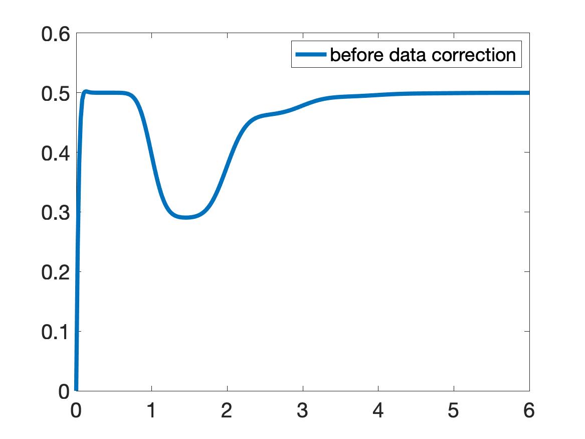
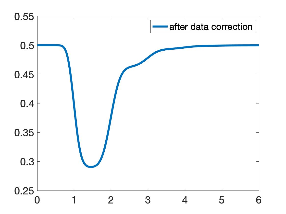
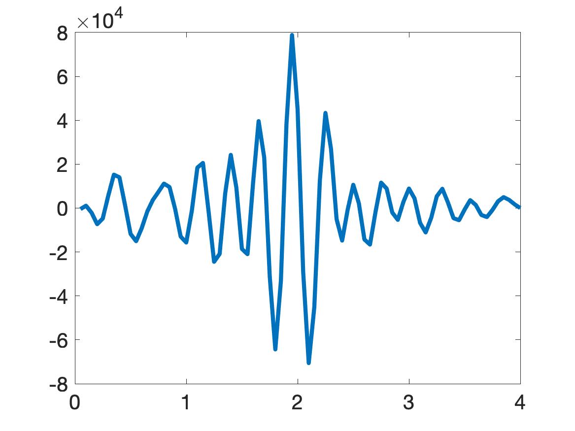
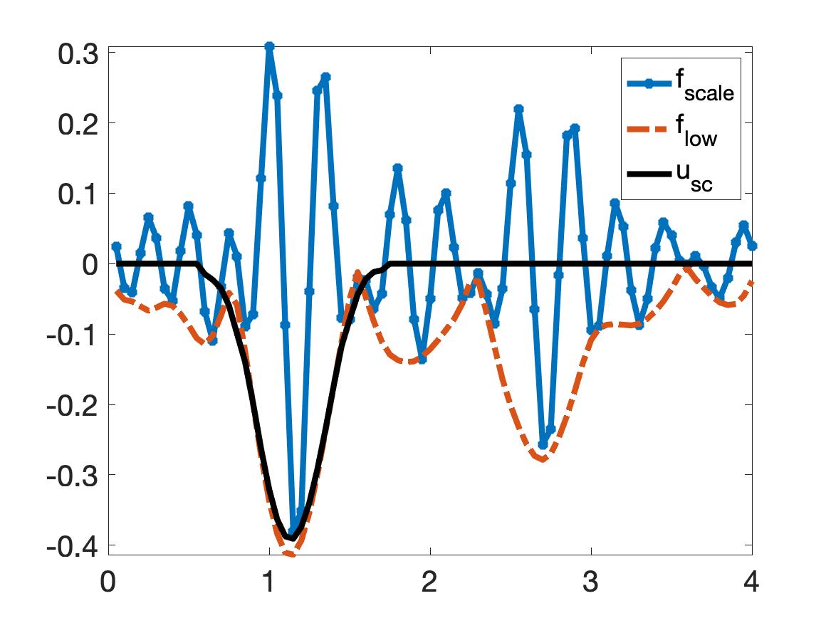
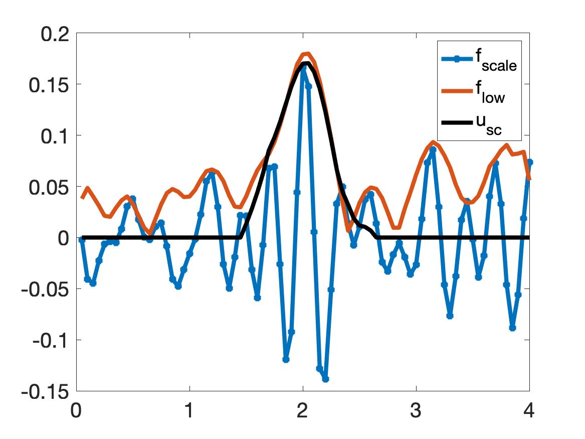
By matching the absorbing boundary conditions in (6.1) and the absorption conditions (2.11)–(2.12) in Lemma 2.2, we see that the solution of problem (1.2) can be approximated on $[-a,a]\times[0,T]$ by the solution of problem (6.1). However, since the Dirac function is replaced by the function $\widetilde{\delta}_{0}$, there is a computational error in the computed function $u$ near $(x=0,t=0)$. It follows from the presentation (2.5) that when $x$ is in a small neighborhood of $\left\{x=0\right\}$, where $c(x)=1$, the function $u(x,t)=1/2$ if $t<|\tau(x)|$. One can see in Figure 2a that $u(0,t)<\frac{1}{2}$ when $t$ small. Therefore, we simply correct this error by reassigning $u(x,t)=\frac{1}{2}$ when $x$ and $t$ are near 00. The function $u(0,t)$ after this data correction process is displayed in Figure 2b. In our computational program, we set $u(x,t)=\frac{1}{2}$ when $(x,t)\in[0,0.0067]\times[0,0.26].$

Refer to caption
(a)
Refer to caption
(b)
Figure 2: Illustration of the process of correcting the data near $(x=0,t=0).$ We know that when $x$ is small, $c(x)=1$. Therefore by (2.5), $u(x,t)=\frac{1}{2}$ for $t<|\tau(x)|.$ We, therefore, set $u(x,t)=\frac{1}{2}$ for $x$ and $t$ small. Figure 2a and figure 2b are the graphs of the function $u(0,t)$ before and after, respectively, this reassignment. These functions are taken from Test 3 in subsection 6.3.

Having the function $u$ in hands, we compute the functions $g_{0}(t)=u(0,t)$ and $g_{1}(t)=u_{x}(0,t)$ easily. These are the computationally simulated data for the inverse problem. In the next section, we present the implementation of the convexification method to solve problem (2.22).

Remark 6.1.

Let $\delta>0$ be the noise level. We arrange the noisy data by

$$g_{0}^{\delta}=g_{0}(1+\delta\mbox{rand})\quad\mbox{and}\quad g_{1}^{\delta}=g_{1}(1+\delta\mbox{rand}),$$

where rand is the function that generates uniformly distributed random numbers in the range $[-1,1].$ The boundary constraints in (2.22) involve the derivative of $g_{0}^{\delta}$. We compute $(g_{0}^{\delta})^{\prime}$ by the Tikhonov regularization method. The Tikhonov regularization method is well-known. We, therefore, do not describe this step here. In all numerical tests of subsection 6.3, the noise level is $\delta=0.05,$ i.e. $5\%.$

6.2 The numerical implementation of the convexification method

We first present our way to compute the function $q^{(0)}\in H$ in step 1 in Algorithm 1 to initiate the process of minimizing the objective functional $J_{\lambda,\alpha,\beta}.$ In the case when $c\equiv 1$, due to (2.5), the function $q(x,0)=1/2$ for all $x\in[\epsilon,M].$ Hence, it is natural to set $q^{(0)}(x,0)=1/2$ for all $x\in[\epsilon,M].$ We next find $q^{(0)}(x,t)$ for $t>0$ by solving the linear partial differential equation obtained by removing the third term in the left hand side of the equation in (2.22). More precisely, we set $q^{(0)}$ as the solution of:

$$\left\{\begin{array}[]{ll}q_{xx}^{(0)}(x,t)-2{q_{xt}^{(0)}(x,t)}=0,&(x,t)\in(\epsilon,M)\times(0,T),\\ q^{(0)}(\epsilon,t)=g_{0}(t+\epsilon),&t\in[0,T],\\ q_{x}^{(0)}(\epsilon,t)=g_{1}(t+\epsilon)+g_{0}^{\prime}(t+\epsilon),&t\in[0,T],\\ q_{x}^{(0)}(M,t)=0,&t\in[0,T].\end{array}\right.$$ (6.2)

Denote $Q^{(0)}(x,t)=q_{x}^{(0)}(x,t)$. It follows from (6.2) that

$$\left\{\begin{array}[]{ll}Q_{x}^{(0)}(x,t)-2Q_{t}^{(0)}(x,t)=0,&(x,t)\in(\epsilon,M)\times(0,T),\\ Q^{(0)}(\epsilon,t)=g_{1}(t+\epsilon)+g_{0}^{\prime}(t+\epsilon),&t\in[0,T],\\ Q^{(0)}(M,t)=0,&t\in[0,T].\end{array}\right.$$ (6.3)

The equation in (6.3) is a linear transport equation for $Q^{(0)}$ with constant coefficients. Since boundary value problem (6.3) is over-determined, we solve it by the quasi-reversibility method, which was first introduced in [40]. More precisely, we minimize the functional $I(Q),$

$$I(Q)=\int_{\Omega}|Q_{x}(x,t)-2Q_{t}(x,t)|^{2}dxdt+\int_{0}^{T}|Q(\epsilon,t)-g_{1}(t+\epsilon)+g_{0}^{\prime}(t+\epsilon)|^{2}dt$$
$$+\int_{0}^{T}|Q(M,t)|^{2}dt+\eta\|Q\|_{H^{2}(\Omega_{T})},$$ (6.4)

where $\eta$ is a small number for $Q^{(0)}$. In our computations, $\eta=10^{-11}.$

We draw the reader’s attention to the survey [22] about the quasi-reversibility method for the existence and uniqueness of the minimizers of similar functionals as well as for the convergence theorems of the minimizers to the exact solutions. This method was considered in [22] for a variety of ill-posed problems, including overdetermined ones and for a variety of PDEs. Considerations for (6.4) are quite similar. Thus, we do not discuss these questions here for brevity.

Having $Q^{(0)}(x,t)$ at hands, we find the function $q^{(0)}(x,t)$ as:

$$q^{(0)}(x,t)=q^{(0)}(\epsilon,t)+\int_{\epsilon}^{x}Q^{(0)}(y,t)dy=g_{0}(t+\epsilon)+\int_{\epsilon}^{x}Q^{(0)}(y,t)dy,$$

for all $(x,t)\in[\epsilon,M]$. Following (2.25), we set the corresponding approximation for the unknown coefficient $c\left(x\right)$ as:

$$c_{\mathrm{init}}(x)=\frac{1}{16(q^{0})^{4}(x,0)},\quad\mbox{for all }x\in[\epsilon,M].$$ (6.5)

We now describe our implementation for Step 2 in Algorithm 1. This is to minimize the functional $J_{\lambda,\alpha,\beta}$. To work without the boundary constraints in (2.22) and to speed up computations the process, we add to the functional $J_{\lambda,\alpha,\beta}$ the boundary terms and minimize the resulting function without boundary constraints. In addition, although in our theory we use the $H^{5}\left(\Omega_{T}\right)-$norm for the regularization term, in computations we use the simpler to implement $H^{2}\left(\Omega_{T}\right)-$norm. The resulting functional is still named as $J_{\lambda,\alpha,\beta}$, and it is given by

$$J_{\lambda,\alpha,\beta}(q)=\int_{\Omega_{T}}e^{-2\lambda(x+\alpha t)}\Big{|}q_{xx}(x,t)-q_{xt}(x,t)\frac{1}{2q^{2}(x,0)}+q_{t}(x,t)\frac{q_{x}(x,0)}{2q^{3}(x,0)}\Big{|}^{2}dxdt$$
$$+\int_{0}^{T}e^{-2\lambda(x+\alpha t)}|q(\epsilon,t)-g_{0}(t+\epsilon)|^{2}dt$$
$$+\int_{0}^{T}e^{-2\lambda(x+\alpha t)}\left|q_{x}(\epsilon,t)-g_{1}(t+\epsilon)-g_{0}^{\prime}(t+\epsilon)\right|^{2}dt+\beta\|q\|_{H^{2}(\Omega_{T})}^{2}.$$ (6.6)

Functional (6.6) can be minimized via a number of optimization packages. We do so using the ready-to-use optimization toolbox of Matlab. More precisely, we use the command “fminunc” of Matlab to find the minimizer of $J_{\lambda,\alpha,\beta}$. The command “fminunc” has its own stopping criteria. In our experience that this command stops when either

  1. 1.

    Either a minimizer is found (Matlab lets us know if a minimizer is found).

  2. 2.

    Or the number of times Matlab computes the objective function reaches a default maximum number determined by Matlab.

In the case 1, we take the output of “fminunc” as the function $q_{\mathrm{comp}}$ and compute $c_{\mathrm{comp}}$ as in Step 3 of Algorithm 1. If “fminunc” stops due to the reason of case 2, we understand that the minimizer is not yet reached. Then, we apply an additional step to speed up the process. Let $\tilde{q}\left(x,t\right)$ denotes the output of “fminunc”. We set

$$\tilde{c}\left(x\right)=\frac{1}{16\tilde{q}^{4}\left(x,0\right)},\quad\mbox{for all }x\in[\epsilon,M].$$ (6.7)

Next, we solve the following linear boundary value problem with over-determined boundary data

$$\left\{\begin{array}[]{ll}\tilde{q}_{xx}^{(1)}(x,t)-\frac{\tilde{q}_{xt}^{(1)}(x,t)}{2\tilde{q}^{2}(x,0)}+\frac{\tilde{q}_{t}(x,t)\tilde{q}_{x}(x,0)}{2\tilde{q}^{3}(x,0)}=0,&(x,t)\in(\epsilon,M)\times(0,T),\\ \tilde{q}^{(1)}(\epsilon,t)=g_{0}(t+\epsilon),&t\in[0,T],\\ \tilde{q}_{x}^{(1)}(\epsilon,t)=g_{1}(t+\epsilon)+g_{0}^{\prime}(t+\epsilon),&t\in[0,T],\\ \tilde{q}_{x}^{(1)}(M,t)=0,&t\in[0,T].\end{array}\right.$$ (6.8)

for a function $\tilde{q}^{(1)}$. Again, we use the quasi-reversibility method via minimizing the obvious analog of the functional $I(Q)$ in (6.4). Next, we set

$$\tilde{c}_{1}(x)=\frac{1}{16(\tilde{q}^{(1)})^{4}(x,0)},\quad\mbox{for all }x\in[\epsilon,M].$$ (6.9)

We next minimize the functional $J_{\lambda,\alpha,\beta}$ in (6.6) again by “fminunc” with the initial input $q^{(0)}=\tilde{q}^{(1)}$. If the minimizer is found, then we stop. If, however, it is not found, then we compute a new function $\tilde{c}(x)$ in (6.7) and proceed as above. This process stops when $\|\tilde{c}-\tilde{c}_{1}\|_{L^{\infty}(\epsilon,M)}<10^{-3}.$ The final reconstruction of the function $c$ is $c_{\mathrm{comp}}\left(x\right)=\tilde{c}\left(x\right).$ By our computational experience, we need no more than one (1) correction (6.8) for the initial input.

Remark 6.3. In our computations, the parameters for the Carleman Weight Function are $\lambda=2$, $\alpha=0.3$, the regularization parameter $\beta=10^{-9}$. $T=6$, $\epsilon=0$ and $M=3$. In (5.40$\alpha T>2M.$ But this condition is not necessary to impose in our numerical experiments. These numbers are chosen by a trial-and-error procedure. This means that we try many sets of these parameters to get the best numerical result for one test, which we call “reference test” (test 1 in subsection 6.3). Then we use the same parameters for all other tests, including the tests with experimental data. In theory, $\lambda$ should be a large number. Here, we choose $\lambda=2$ because this value is sufficient to obtain satisfactory numerical results. If $\lambda$ is too large, then the Carleman Weight Function decays too rapidly. This causes many difficulties in numerics; especially, on the computing time. In fact, a similar issue takes place in any asymptotic theory when it is applied to real computations. Indeed, such a theory basically says that “If a certain parameter X is sufficiently large, then a certain “good thing” takes place”. However, when computing, one needs to estimate X computationally since theoretical estimates usually more pessimistic than numerical ones.

6.3 Numerical results for computationally simulated data

We present five (5) numerical examples to test our convexification method. The obtained results are displayed in Figure 3.

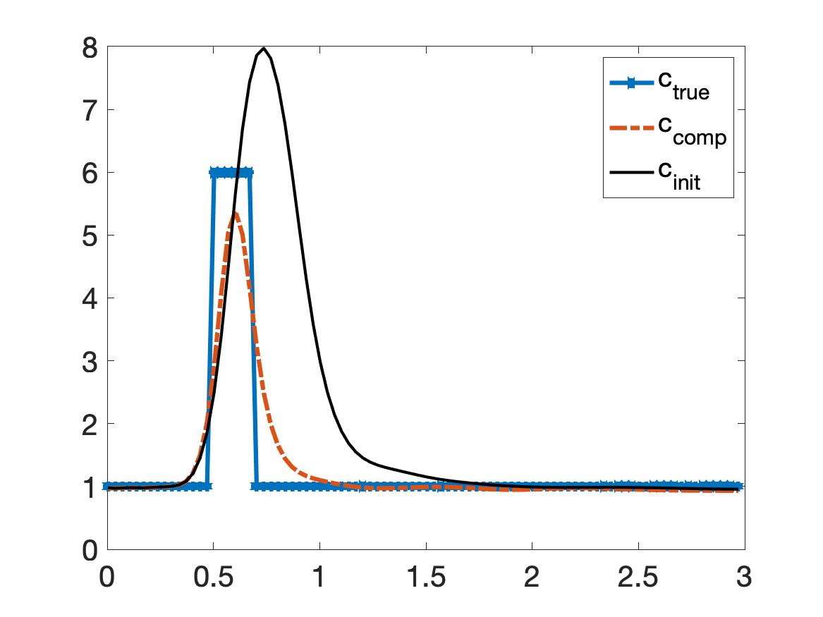
Test 1. In this test, we consider the case of one inclusion with a high inclusion/background contrast. The true function $c\left(x\right)$ is given by

$$c_{\mathrm{true}}(x)=\left\{\begin{array}[]{ll}1+10e^{\frac{(x-0.5)^{2}}{(x-0.5)^{2}-0.2^{2}}}&\mbox{if }|x-0.5|<0.2,\\ 1&\mbox{otherwise}.\end{array}\right.$$

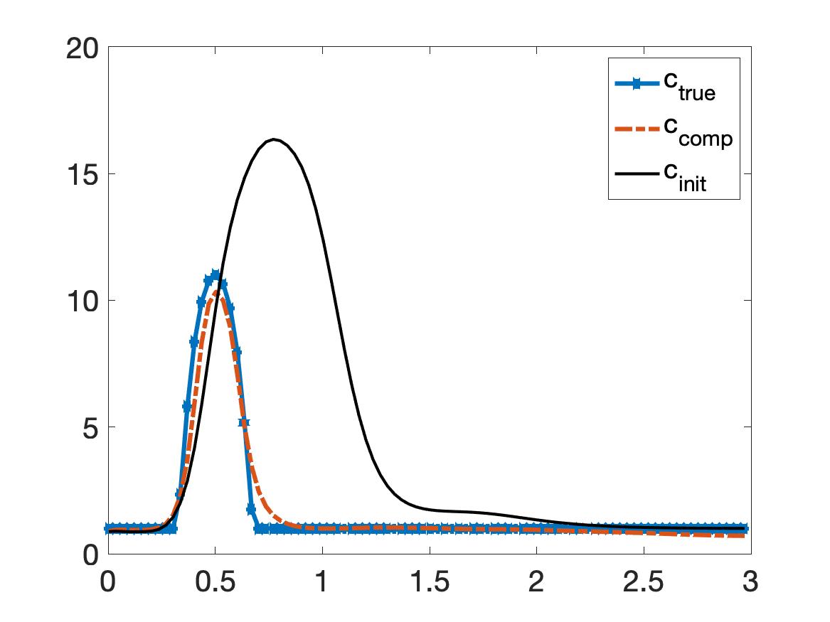
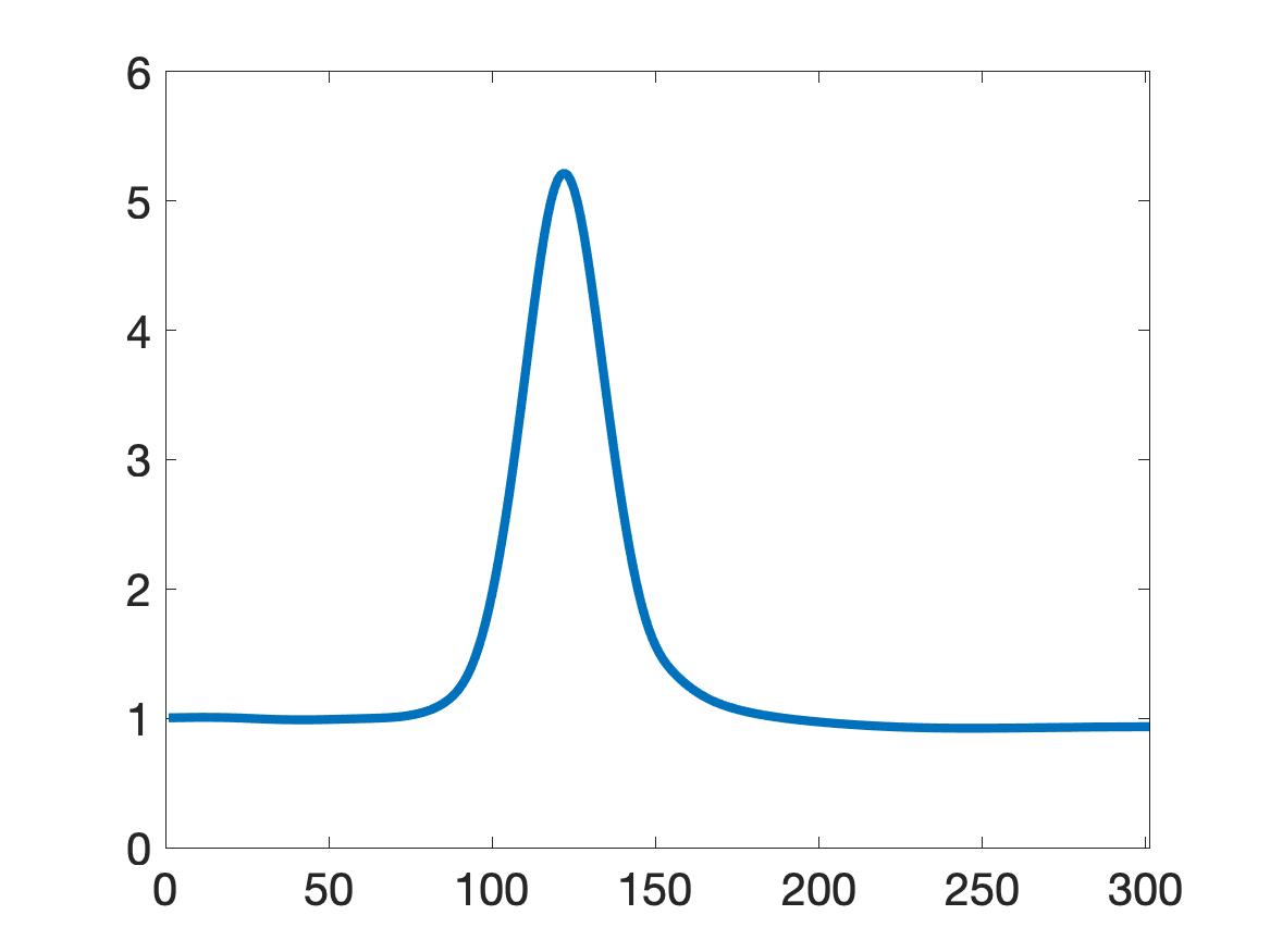
In this test, we detect one object with a high dielectric constant with the size 0.4 and the center located at $0.5$. Although the inclusion/background contrast here is $11/1=11,$ which is high, our method provides good numerical results without any knowledge of $c_{\mathrm{true}}$ inside of $[\epsilon,M]$. The numerical solution of this test is displayed in Figure 3a. In this test, the function $c_{\mathrm{init}}$ obtained by (6.5) somewhat provides the information about $c_{\mathrm{true}},$ but it is still far away from $c_{\mathrm{true}}.$ The final reconstruction quite exactly indicates the position of the “inclusion”. The maximal value of the computed function $c\left(x\right)$ in the inclusion is 10.43 (relative error 5.2%). This value is accurate since we have the the noise level $\delta=5\%$.

Test 2. We test a more complicated function $c_{\mathrm{true}}.$ In this test, the dielectric constant is a smooth function $c\left(x\right)$ with two (2) inclusions. The function $c_{\mathrm{true}}$ is given by

$$c_{\mathrm{true}}(x)=\left\{\begin{array}[]{ll}1+3e^{\frac{(x-0.5)^{2}}{(x-0.5)^{2}-0.2^{2}}}&\mbox{if }|x-0.5|<0.2,\\ 1+5e^{\frac{(x-1.4)^{2}}{(x-1.4)^{2}-0.3^{2}}}&\mbox{if }|x-1.4|<0.3,\\ 1&\mbox{otherwise}.\end{array}\right.$$

This test is challenging since the maximal value of the function $c_{\mathrm{true}}(x)$ in each inclusion is high (4 and 6). The left inclusion is blocked by the right inclusion in the in the view of the source and the detector, both of which are located at $\left\{x=0\right\}$. The graphs of the true function $c(x),$ initial and computed solutions are displayed in Figure 3b. The function $c_{\mathrm{init}}$ computed by (6.5) somewhat provides a guess about the shape of $c_{\mathrm{true}}$ but is still far away from $c_{\mathrm{true}}.$ The final reconstruction is good. The computed locations of both inclusions are satisfactory. The maximal value of the computed function $c\left(x\right)$ in the left inclusion is 3.40 (relative error 15%). The maximal value of the computed function $c(x)$ in the right inclusion is 5.16 (relative error 14%).

Test 3. We now consider the case when $c_{\mathrm{true}}(x)$ is a discontinuous step function,

$$c_{\mathrm{true}}(x)=\left\{\begin{array}[]{ll}6&\mbox{if }|x-0.6|<0.1,\\ 1&\mbox{otherwise.}\end{array}\right.$$

This test is an interesting one. It shows that the convexification method is stronger than what we can prove in the theory in the sense that the smoothness condition of the function $c\left(x\right)$ can be relaxed in numerical studies, although this condition is used in the theoretical part. The true, initial and the computed solutions of Problem 1.1 are displayed in Figure 3c. The initial solution obtained by (6.5) somewhat indicates the inclusion but both the location and the value of the dielectric constant inside the inclusion are far from correct ones. However, both the location and the computed dielectric constant meet the expectation in the final reconstruction of the function $c$. The maximal value of the computed function $c\left(x\right)$ is 5.6 (relative error is 6.7%).

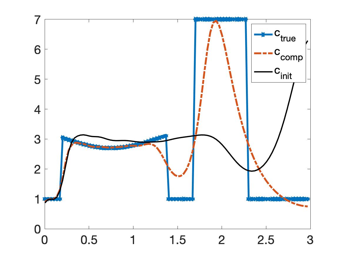
Test 4. We consider the case of three inclusions. As in the previous example, the dielectric constant function $c$ in this case is a discontinuous one. It is given by

$$c_{\mathrm{true}}(x)=\left\{\begin{array}[]{ll}3&\mbox{if }|x-0.3|<0.1,\\ 5&\mbox{if }|x-0.8|<0.15,\\ 7&\mbox{if }|x-1.5|<0.2,\\ 1&\mbox{otherwise}.\end{array}\right.$$

Reconstructing this function $c\left(x\right)$ is challenging. In fact, since we only measure the data at $x=\epsilon$, in the view of the detector, the second and third inclusions are blocked by the first one. Nevertheless, our method works well. The numerical solutions are displayed in Figure 3d. As in the previous examples, the initial solution $c_{\mathrm{init}}\left(x\right)$ provides some information about the function $c_{\text{true}}\left(x\right),$ but the error is large. This error is corrected by our convexification method. The final reconstruction successfully shows locations of all three inclusions. The maximal values of the computed function $c\left(x\right)$ in each inclusion are good. The computed maximal value of $c\left(x\right)$ in the left inclusion is 2.8 (relative error 6.7%). The computed maximal value of $c\left(x\right)$ in the middle inclusion is 4.6 (relative error 8.0%). The computed maximal value of $c\left(x\right)$ in the right inclusion is 6.9 (relative error 1.4%).

Test 5. We now test another interesting case, in which the true dielectric constant includes two inclusions. The function $c\left(x\right)$ in the first one is a smooth function, and in the second one it has a constant value. The true dielectric constant is given by

$$c_{\mathrm{true}}=\left\{\begin{array}[]{ll}3+0.3\sin(\pi(x-1.25))&\mbox{if }|x-.08|<0.6,\\ 7&\mbox{if }|x-2|<0.3,\\ 1&\mbox{otherwise.}\end{array}\right.$$

The numerical solution of this test is given in Figure 3e. The initial solution $c_{\mathrm{init}}$ obtained by (6.5) is far away from the true function $c\left(x\right)$. It might not contain any valuable information of the true function $c_{\text{true}}\left(x\right)$. In the next step, after applying the convexification method, we get a good reconstruction of $c_{\mathrm{true}}\left(x\right)$. The curve in the first inclusion locally coincides with the true one. The position and the computed function $c\left(x\right)$ of the second inclusion are also accurate. The computed maximal value of $c\left(x\right)$ in the second inclusion is 6.9 (relative error 1.4%).

Refer to caption
(a) Numerical result of test 1 for simulated data with $5\%$ noise
Refer to caption
(b) Numerical result for test 2 from simulated data with $5\%$ noise
Refer to caption
(c) Numerical result for test 3 from simulated data with $5\%$ noise
Refer to caption
(d) Numerical result for test 4 from simulated data with $5\%$ noise
Refer to caption
(e) Numerical result for test 5 from simulated data with $5\%$ noise
Figure 3: The true spatially distributed dielectric constant function $c_{\mathrm{true}}$, its initial version $c_{\mathrm{init}}$ computed by (6.5) and its final reconstruction $c_{\mathrm{comp}}$ by our convexification method. It is evident that in all cases, the initial solution $c_{\mathrm{init}}$ computed by (6.5) already carries some information of $c_{\mathrm{true}}$. The following iterative steps significantly improve the positions of “inclusions” and their values. Especially, in test 5 (Figure 3e), the convexification method successfully reconstructs the curves in the inclusion in the left.

Remark 6.4. In this section, we have tested our convexification method for multiple cases. The numerical results show that our method is robust, since it can be used for the cases when the dielectric constant has high contrasts, single or multiple inclusions, and a complicated form. More importantly, we obtain those satisfactory results without requiring any initial guess.

7 Numerical Studies of Experimental Data

We use the data collected by the Forward Looking Radar built in the US Army Research Laboratory [49]. The goal of this radar is to detect and identify flash explosive-like targets, such as antipersonnel land mines and improvised explosive devices. These targets can be both buried on a few centimeters depth in the ground and located in air, i.e. above the ground.

The device has an emitter and sixteen (16) detectors. The emitter sends out only one component of the electric field forward the area that covers the object and the detectors collect the back scattering electric signal (voltage) in the time domain. The same component of the electric field is measured as the one which is generated by the emitter, see Figure 1 for the schematic diagram of data collection. See the comment about the validity of the data at the beginning of [35, Section 2]. The step size in time is 0.133 nanosecond. The backscattering data in the time domain are collected when the distance between the radar and the target varies from 8 to 20 meters. We then take the average of these data with respect to both the position of the radar and those 16 detectors and use as the 1D data to test our convexification method. Due to this “average” of the data, we are unable to find the location of the target. The location can be found by using the Ground Positioning System (GPS). The error in each of horizontal coordinates does not exceed a few centimeters, which is sufficient for practical purposes. When the target is under the ground, the GPS provides the distance between the radar and a point on the ground located above the target. As to the depth of a buried target, it is not of a significant interest, since horizontal coordinates are known and it is also known that the depth does not exceed 10 centimeters. We refer to [49] for more details about the data collection process. We refer to previous works of our group in [13, 35, 29, 30, 38, 39, 53] where these experimental data were treated by different inversion algorithms for Coefficient Inverse Problems.

Hence, the interest here is to compute the values of the dielectric constants of the targets using these data. Indeed, we hope that in the future knowledge of dielectric constants, being combined with the knowledge of other parameters of targets, might help to reduce the false alarm rate. An interesting feature of our data is that they were collected in the field, rather than in a simpler case of a laboratory. Besides, all targets were surrounded by clutter.

As in all previous our above cited works on these data, we have calculated the relative spatially distributed dielectric constant $c_{\mathrm{rel}}(x)$ of the medium including the background (air or ground) and the target. The function $c_{\mathrm{rel}}(x)$ is given by

$$c_{\mathrm{rel}}(x)=\left\{\begin{array}[]{ll}\frac{c_{\mathrm{target}}}{c_{\mathrm{bckgr}}}&\mbox{if }x\in D,\\ 1&\mbox{otherwise}\end{array}\right.$$ (7.1)

where $D$ is a sub interval of $[\epsilon,M]$ which is occupied by the target. Here, $c_{\mathrm{target}}$ is the dielectric constant of the target and $c_{\mathrm{bckgr}}$ is the dielectric constant of the background. If the background is air, then $c_{\mathrm{bckgr}}=1$. If the background is dry sand, then $c_{\mathrm{bckgr}}\in(3,5)$ (see table of dielectric constants listed on a website of Honeywell, https://goo.gl/kAxtzB). Our inverse solver in this paper is suitable to compute $c_{\mathrm{rel}}$ given the backscattering data. The computed $c_{\mathrm{target}}$ follows.

7.1 Data preprocessing

It was observed in previous above cited publications of this group about inversion of these experimental data that there is a significant discrepancy between the computationally simulated data and experimentally collected data. Hence, the first step to invert these data is to preprocess them. So that the preprocessed data and the simulated data would look similarly. We are doing this by scaling and truncating. We consider two cases.

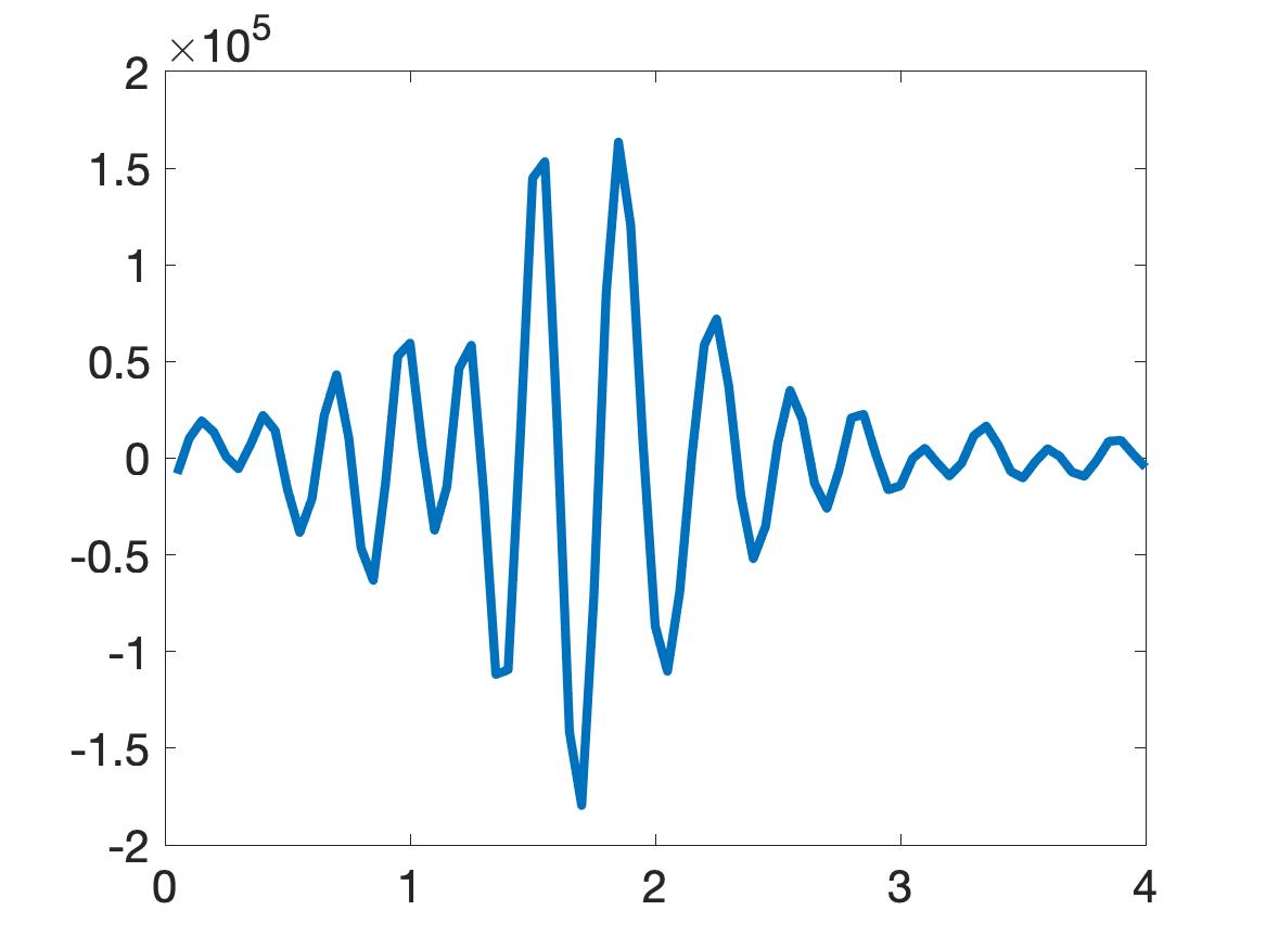
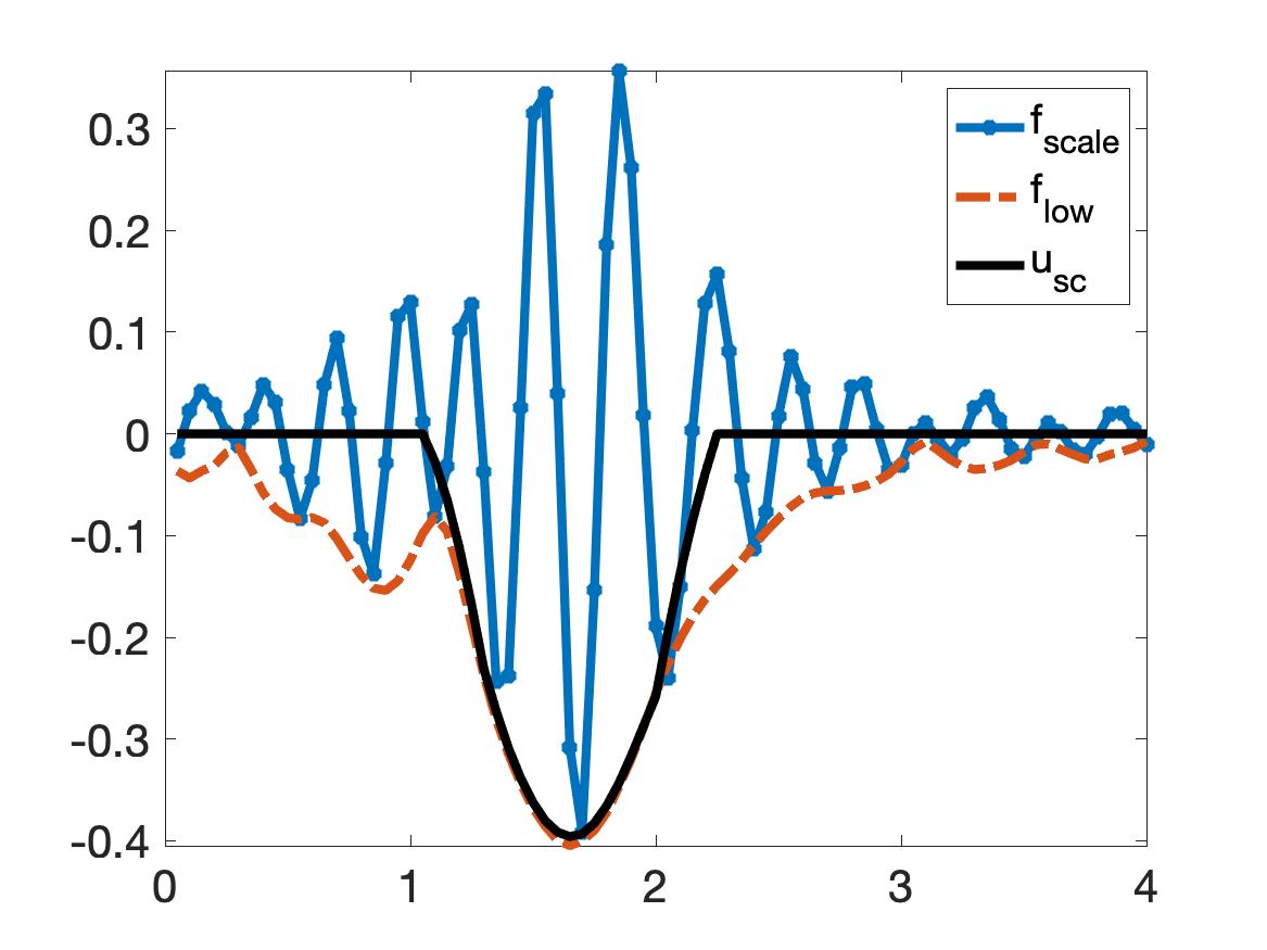
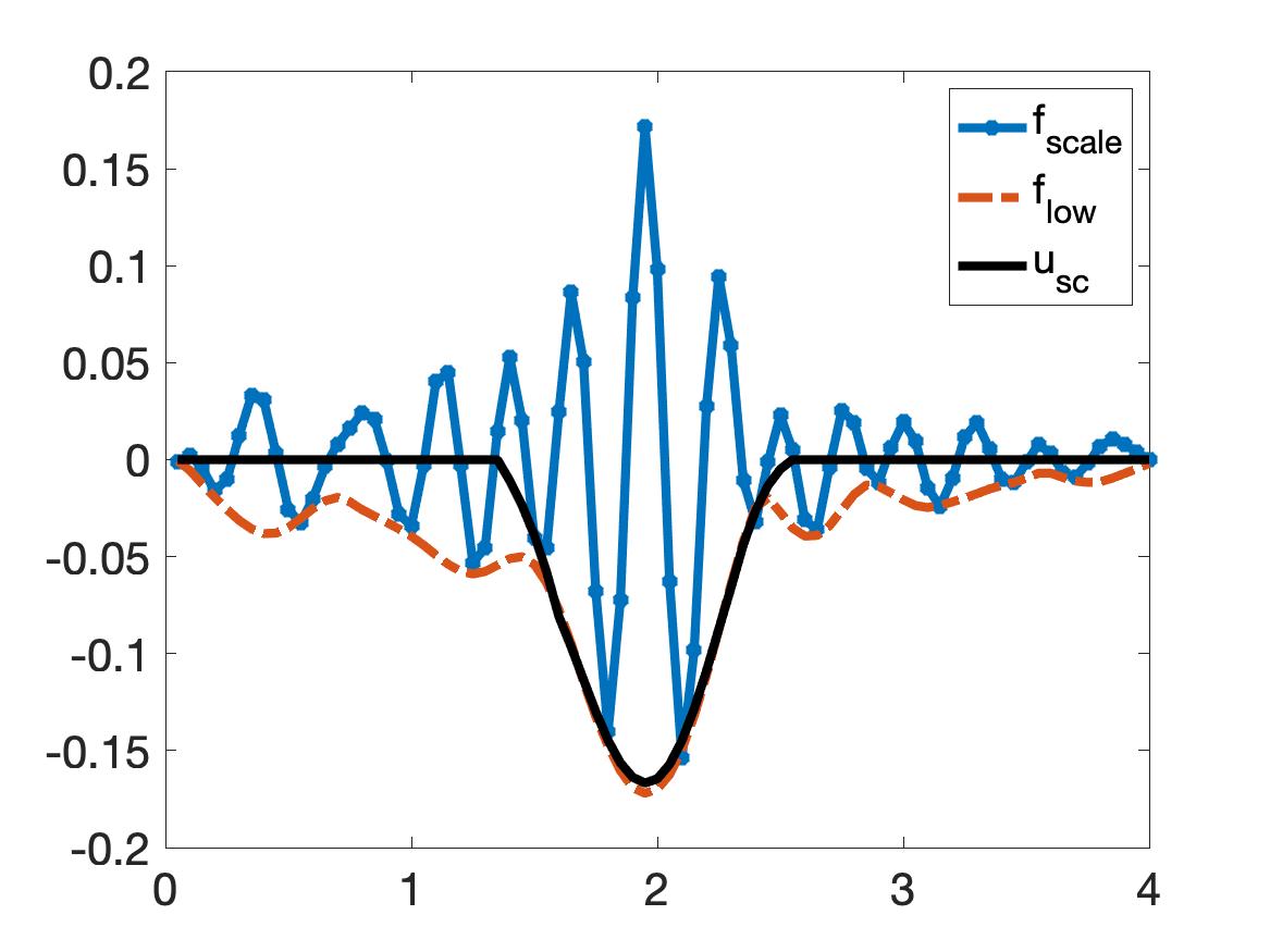
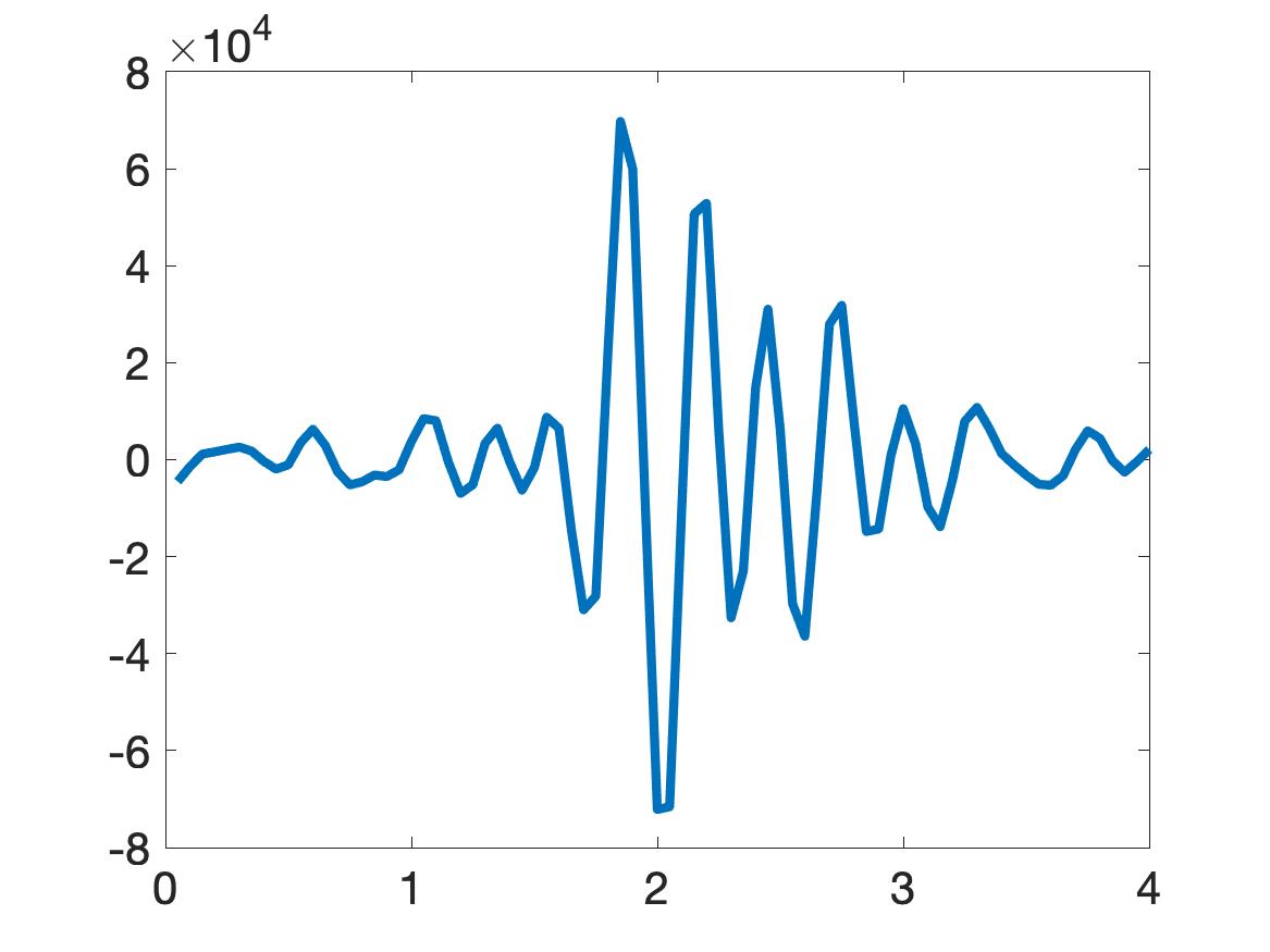
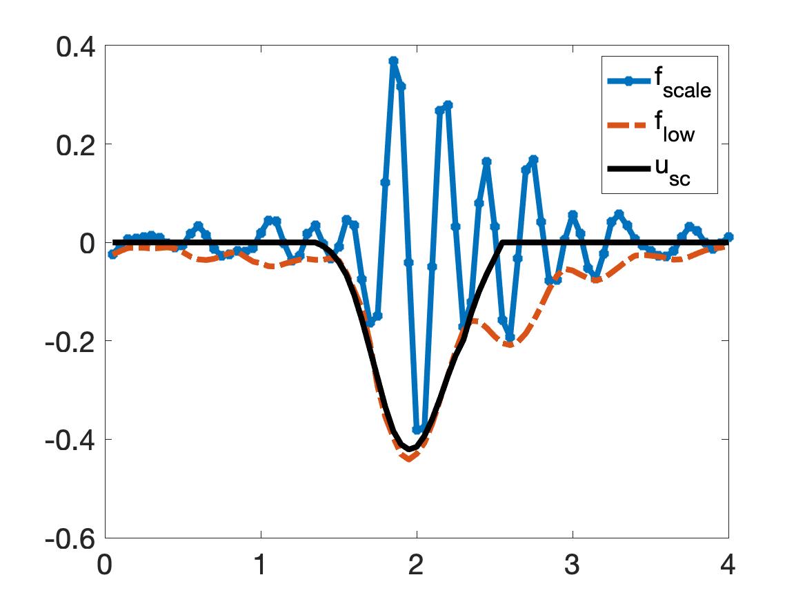
1. The case when the targets are in air. We first notice that the magnitude of the raw experimental data $f_{\mathrm{raw}}$ is large while that of the simulated data is small. This difference is due to the fact that we scale the speed of light in the air to be 1. Thus, we compute a “scaling factor”. To do so, we have to know the true solution of one set of data generated by a known target. This target is called the reference object. We choose the reference object as a bush with its dielectric constant about 6.5 [35]. We then generate a corresponding simulated data, named as $f_{\mathrm{sim}}$. The scaling factor $\mu$ is determined as $\mu\|f_{\mathrm{raw}}\|_{L^{\infty}}=\|f_{\mathrm{sim}}\|_{L^{\infty}}$. The computed scaling factor is $\mu=459420$. We use the same scaling factor for other tests. The scaled data $f_{\mathrm{scale}}=\mu f_{\mathrm{raw}}.$ We next truncate the data. Since the object is placed in the air, then $c_{\mathrm{bckgr}}=1$ and $c_{\mathrm{target}}>1$. As seen in Figure 2, the value of the value of the total simulated wave is less than $0.5:$ 0.5 should be subtracted, see the first term in the right hand side of (2.5). This term is responsible for the incident wave. Therefore, the back scattering wave is non-positive. We thus cut off all positive values of $f_{\mathrm{scale}}$ by bounding it by a lower envelop for the scaled data, see Figures 4b and 4e for illustrations of the envelops. This lower envelop is the graph of the function named $f_{\mathrm{low}}(t)$. We next truncate $f_{\mathrm{low}}$ because we known that before and after the backscattering wave hits and then passes the detector, the data is 00. This truncating step is as follows. Let $t_{\mathrm{min}}$ be the absolute minimizer of $f_{\mathrm{low}}(t)$. We keep the value of $f_{\mathrm{low}}(t)$ in a neighborhood of $t_{\mathrm{min}}$, say $(t_{\mathrm{min}}-10\delta_{t},t_{\mathrm{min}}+10\delta_{t})$ where $\delta_{t}$ is the step size in time, and re-assign the value of $f_{\mathrm{low}}(t)=0$ outside this neighborhood. The obtained function is the backscattering wave $u_{\mathrm{sc}}$. Due to Lemma 2.6, the total wave at the detector is $u_{\mathrm{sc}}+0.5.$ See Figures 4a, 4b, 4d and 4e for the results of data preprocessing.

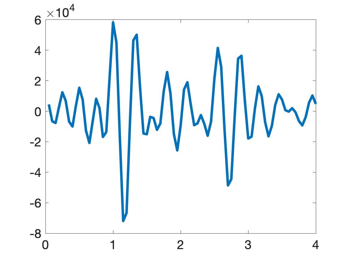
2. Consider the case when the targets are buried under the ground. The background in this case is dry sand. Its dielectric constant is in the interval $\left[3,5\right].$ We take the average and choose $c_{\mathrm{bckgr}}=4.$ We first scale the raw data in the same manner as in case 1 in which the target is placed in the air. This means that we must know the true solution of one set of data, generated by a reference target. We use a metal box with its dielectric constant about 18.5 [35] as the reference target. Then, we find a scaling factor $\mu$ such that $\mu f_{\mathrm{raw}}$ have the same magnitude as the simulated data. The relative dielectric constant for this reference object is $c_{\mathrm{rel}}(x)=4.6$, see (7.1). The computed scaling factor is $\mu=189445.$ As in case 1, the scaled data is denoted by $f_{\mathrm{scale}},$ which is $\mu f_{\mathrm{raw}}.$ If the dielectric constant of the target $c_{\mathrm{target}}$ is larger than that of the background $c_{\mathrm{bckgr}}$, then the values of the simulated data are less than 0.5 and, hence, the simulated backscattering wave is non-positive. In this case, we bound $f_{\mathrm{scale}}$ by its lower envelop, called $f_{\mathrm{low}}$. If $c_{\mathrm{target}}$ is smaller than $c_{\mathrm{bckgr}}$, the simulated data is larger than 0.5. In this case, the simulated backscattering wave is non-negative. We hence bound $f_{\mathrm{scale}}$ by its upper envelop, called $f_{\mathrm{up}}$. A question arising immediately: how can we know if the dielectric constant of the target is smaller or larger than that of the background. We answer this question by experimental observation we got when working with these experimental data in the past [35]. We look at the data and find the three extrema with largest absolute values. If the middle extremal value among these three is a minimum, then $c_{\mathrm{target}}>c_{\mathrm{bckgr}}$. If the middle extreme value is a maximum, then $c_{\mathrm{target}}<c_{\mathrm{bckgr}}$. The reader can compare the raw data in Figures 5a, 5d vs. Figure 5g for this phenomenon. We use $f_{\mathrm{envelop}}$ as a common notation for $f_{\mathrm{low}}$ and $f_{\mathrm{up}}$. The last step of data preprocessing is the truncation being applied to $f_{\mathrm{envelop}}$. It is the same as in the truncation step in case 1. We do not repeat this step here.

The result of the data preprocessing step is the function $g_{0}(t)$ for the solution of the inverse problem. In comparison with the problem statement in Problem 1.1, we are missing the knowledge of $g_{1}(t).$ This function is approximated as follows. Using (2.12), we have

$$u_{x}(x,t)=u_{t}(x,t)\quad\mbox{for all }x<0.$$ (7.2)

We accept an error by assuming that (7.2) is valid at 00 in the sense that we take the limit as $x\rightarrow 0^{-}$. Hence, we can approximate $g_{1}(t)=u_{x}(0,t)=u_{t}(0,t)=g_{0}^{\prime}(t)$ for $t>0$.

7.2 Numerical results for experimental data

In this section, we present the numerical results for five (5) tests. The first two tests are to detect targets in the air and the last three tests are to identify targets buried a few centimeters under the ground. Dielectric constants were not measured in these experiments. Therefore, we have no choice but to compare our computed dielectric constants with those listed on the website of Honeywell (Table of dielectric constants, https://goo.gl/kAxtzB). As to the metallic targets, it was numerically established in [38] that one can treat them as dielectrics with the so-called “apparent” dielectric constants whose range is in the interval $\left[10,30\right].$

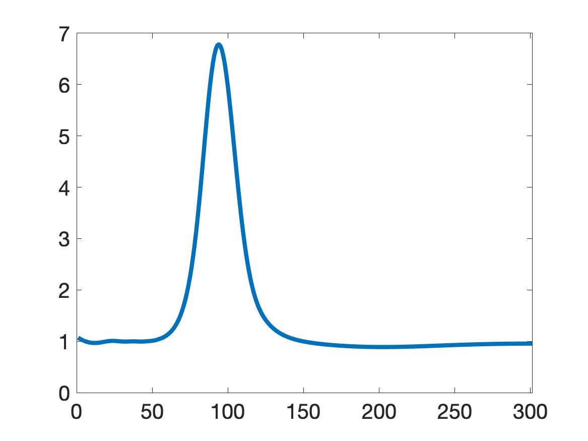
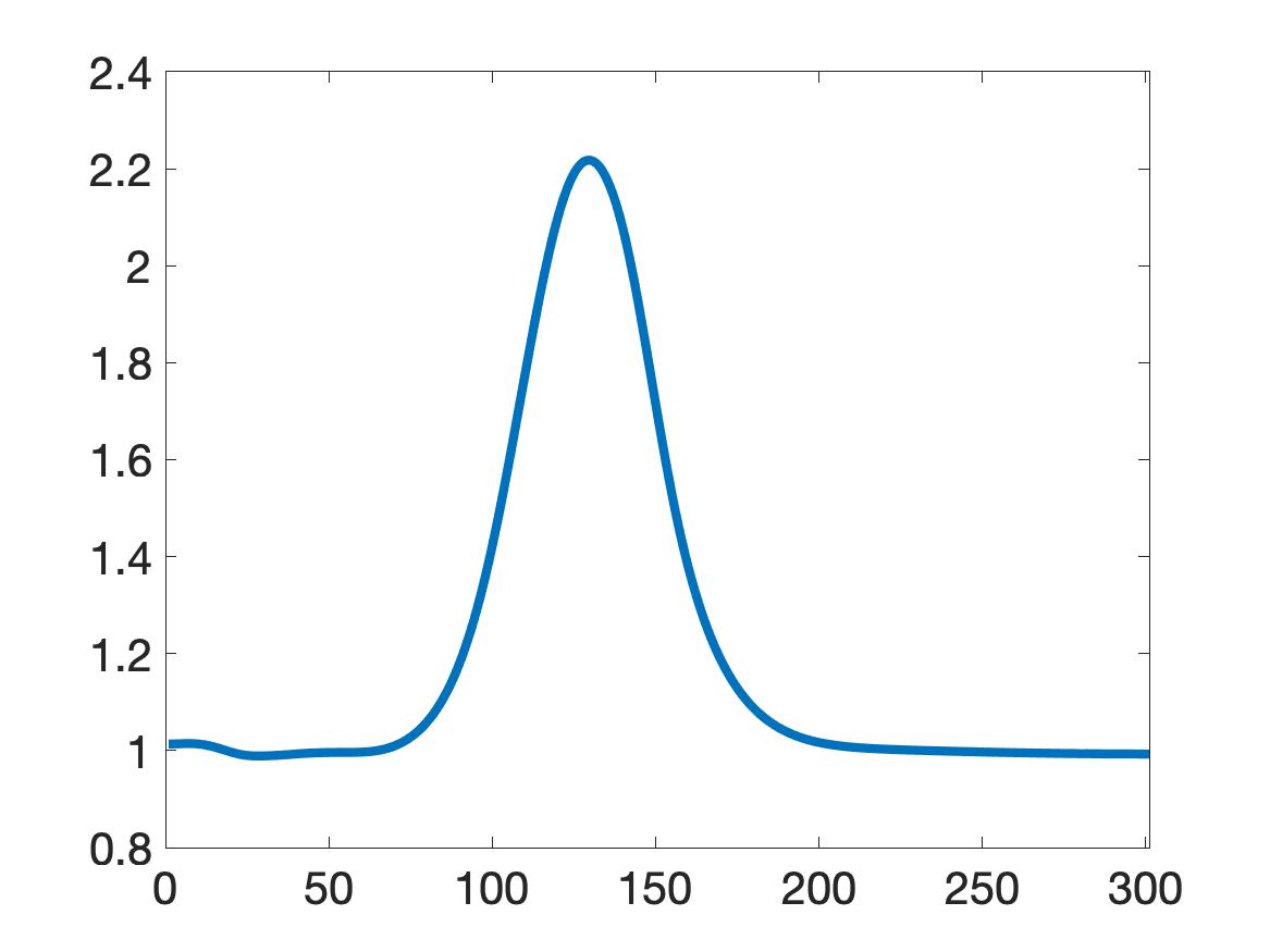
The reconstructed dielectric constants of these targets are summarized in Table 1. It can be seen from Table 1 that the computed dielectric constant of the target and the true one listed on the website of Honeywell (Table of dielectric constants, https://goo.gl/kAxtzB) are having constant values. In the table of dielectric constant of Honeywell, the dielectric constant is not a number. Rather, each dielectric constant of this table is given within a certain intervals. This interval is listed in the last column of Table 1. It is evident that our computed dielectric constants for all targets belong to the intervals of the true dielectric constants. Furthermore, their values are well in the range of those which our group has computed in previous above cited publications, which have worked with these experimental data.

Target $c_{\mathrm{bckgr}}$ computed $c_{\mathrm{rel}}$ $c_{\mathrm{bckgr}}$ computed $c_{\text{target}}$ True $c_{\text{target}}$
Bush 1 6.76 1 6.76 $[3,20]$
Wood stake 1 2.22 1 2.22 $[2,6]$
Metal box 4 5.2 $[3,5]$ $[15.6,26]$ $[10,30]$
Metal cylinder 4 4.7 $[3,5]$ $[14.1,23.5]$ $[10,30]$
Plastic cylinder 4 0.37 $[3,5]$ $[1.11,1.85]$ $\left[1.1,3.2\right]$
Table 1: Computed dielectric constants of five targets
Refer to caption
(a) The time-dependent raw data
Refer to caption
(b) The time-dependent backscattering wave after preprocessing
Refer to caption
(c) Computed dielectric constant. Its maximal value is 6.76.
Refer to caption
(d) The time-dependent raw data
Refer to caption
(e) The time-dependent backscattering wave after preprocessing
Refer to caption
(f) Computed dielectric constant. Its maximal value is 2.2.
Figure 4: The case when the target is in the air. The raw and preprocessed data in the first row correspond to the wave scattered from a bush. The raw and preprocessed data in the second row correspond to the wave scattered from a wood stake. The computed dielectric constants for these two tests meet the expectation since they belong to intervals of their true value, see the last three rows of Table 1.
Refer to caption
(a) The time-dependent raw data
Refer to caption
(b) The time-dependent backscattering wave after preprocessing
Refer to caption
(c) Computed dielectric constant. Its maximal value is 5.2.
Refer to caption
(d) The time-dependent raw data
Refer to caption
(e) The time-dependent backscattering wave after preprocessing
Refer to caption
(f) Computed dielectric constant. Its maximal value is 4.7.
Refer to caption
(g) The time-dependent raw data
Refer to caption
(h) The time-dependent backscattering wave after preprocessing
Refer to caption
(i) Computed dielectric constant. Its minimal value is 0.37.
Figure 5: The case when the target is buried under the ground. The raw and preprocessed data in the first row correspond to the wave scattered from a metal box. The raw and preprocessed data in the second row correspond to the wave scattered from a metal cylinder. The raw and preprocessed data in the third row correspond to the wave scattered from a plastic cylinder. Unlike the tests in the first two rows, we choose the upper envelop in this case when preprocessing the data because $c_{\mathrm{target}}<c_{\mathrm{bckgr}}.$ The computed dielectric constants for these three tests meet the expectation since they belong to intervals of their true value, see the last three rows of Table 1.

8 Summary

We have proposed a new numerical method to solve a highly nonlinear and severely ill-posed coefficient inverse problem. This method is called the convexification. Our technique to prove the convexifying phenomenon heavily relies on a new Carleman estimate, which is proven in Theorem 3.1. The convexification method has the global convergence property. In fact, Theorems 4.1, 5.1-5.3 guarantee that the convexification method delivers a good approximation to the exact solution of the inverse problem without any advanced knowledge of a small neighborhood of that solution. These results are verified numerically for both computationally simulated and experimental data.

Acknowledgments

The work of Klibanov, Le and Loc H. Nguyen , was supported by the US Army Research Laboratory and US Army Research Office grant W911NF-19-1-0044. The authors are grateful to Professors Mikhail Kokurin and Oleg Safronov for their detailed discussions of results of section 4.

References

  • [1] A. B. Bakushinskii, M. V. Klibanov, and N. A. Koshev. Carleman weight functions for a globally convergent numerical method for ill-posed Cauchy problems for some quasilinear PDEs. Nonlinear Anal. Real World Appl., 34:201–224, 2017.
  • [2] L. Baudouin, M. de Buhan, and S. Ervedoza. Convergent algorithm based on Carleman estimates for the recovery of a potential in the wave equation. SIAM J. Nummer. Anal., 55:1578–1613, 2017.
  • [3] L. Baudouin, M. de Buhan, S. Ervedoza, and A. Osses. Carleman-based reconstruction algorithm for the waves. preprint hal-00598876, 2020.
  • [4] L. Beilina and M.  V. Klibanov. Approximate Global Convergence and Adaptivity for Coefficient Inverse Problems. Springer, New York, 2012.
  • [5] L. Beilina and M.  V. Klibanov. Globally strongly convex cost functional for a coefficient inverse problem. Nonlinear Analysis: Real World Applications, 22:272–288, 2015.
  • [6] M Boulakia, M. de Buhan, and E. Schwindt. Numerical reconstruction based on Carleman estimates of a source term in a reaction-diffusion equation. ESAIM: COCV, 2021.
  • [7] A. L. Bukhgeim and M.  V. Klibanov. Uniqueness in the large of a class of multidimensional inverse problems. Soviet Math. Doklady, 17:244–247, 1981.
  • [8] I. M. Gelfand and B. M. Levitan. On determining a differential equation from its spectral function, Amer. Math. Soc. Transl., 2: 253–304, 1955.
  • [9] M. de Hoop, P. Kepley, and L. Oksanen. Recovery of a smooth metric via wave field and coordinate transformation reconstruction. SIAM J. Appl. Math., 78:1931–1953, 2018.
  • [10] V. Isakov. Inverse Problems for Partial Differential Equations. Springer, New York, third edition, 2017.
  • [11] S. I. Kabanikhin, A. D. Satybaev and M. A. Shishlenin. Direct Methods of Solving Multidimensional Inverse Hyperbolic Problems. Walter de Gruyter, 2013.
  • [12] S. I. Kabanikhin, K. K. Sabelfeld, N. S. Novikov and M. A. Shishlenin. Numerical solution of the multidimensional Gelfand–Levitan equation. Journal of Inverse and Ill-Posed Problems, 23: 439–450, 2015.
  • [13] A.L. Karchevsky, M.V. Klibanov, L. Nguyen, N. Pantong, and A. Sullivan. The Krein method and the globally convergent method for experimental data. Applied Numerical Mathematics, 74:111–127, 2013.
  • [14] A. Katchalov, Y. Kurylev, and M. Lassas. Inverse boundary spectral problems. Monographs and Surveys in Pure and Applied Mathematics 123, Chapman Hall/CRC, 2001.
  • [15] V. A. Khoa, G. W. Bidney, M. V. Klibanov, L. H. Nguyen, L. Nguyen, A. Sullivan, and V. N. Astratov. Convexification and experimental data for a 3D inverse scattering problem with the moving point source. Inverse Problems, 36:085007, 2020.
  • [16] V. A. Khoa, M. V. Klibanov, and L. H. Nguyen. Convexification for a 3D inverse scattering problem with the moving point source. SIAM J. Imaging Sci., 13(2):871–904, 2020.
  • [17] M. V. Klibanov, A. Smirnov, V.A. Khoa, A. Sullivan, and L. Nguyen. Through-the-wall nonlinear SAR imaging. to appear on IEEE Transactions on Geoscience and Remote Sensing, see also ArXiv:2008.12622, 2021.
  • [18] M. V. Klibanov. Inverse problems and Carleman estimates. Inverse Problems, 8:575–596, 1992.
  • [19] M. V. Klibanov. Global convexity in a three-dimensional inverse acoustic problem. SIAM J. Math. Anal., 28:1371–1388, 1997.
  • [20] M. V. Klibanov. Global convexity in diffusion tomography. Nonlinear World, 4:247–265, 1997.
  • [21] M. V. Klibanov. Carleman estimates for global uniqueness, stability and numerical methods for coefficient inverse problems. J. Inverse and Ill-Posed Problems, 21:477–560, 2013.
  • [22] M. V. Klibanov. Carleman estimates for the regularization of ill-posed Cauchy problems. Applied Numerical Mathematics, 94:46–74, 2015.
  • [23] M. V. Klibanov. Carleman weight functions for solving ill-posed Cauchy problems for quasilinear PDEs. Inverse Problems, 31:125007, 2015.
  • [24] M. V. Klibanov. Convexification of restricted Dirichlet to Neumann map. J. Inverse and Ill-Posed Problems, 25(5):669–685, 2017.
  • [25] M. V. Klibanov and O. V. Ioussoupova. Uniform strict convexity of a cost functional for three-dimensional inverse scattering problem. SIAM J. Math. Anal., 26:147–179, 1995.
  • [26] M. V. Klibanov, V. A. Khoa, A. V. Smirnov, L. H. Nguyen, G. W. Bidney, L. Nguyen, A. Sullivan, and V. N. Astratov. Convexification inversion method for nonlinear SAR imaging with experimentally collected data. preprint Arxiv:2103.10431, 2021.
  • [27] M. V. Klibanov and A. E. Kolesov. Convexification of a 3-D coefficient inverse scattering problem. Computers and Mathematics with Applications, 77:1681–1702, 2019.
  • [28] M. V. Klibanov, A. E. Kolesov, and D.-L. Nguyen. Convexification method for an inverse scattering problem and its performance for experimental backscatter data for buried targets. SIAM J. Imaging Sci., 12:576–603, 2019.
  • [29] M. V. Klibanov, A. E. Kolesov, L. Nguyen, and A. Sullivan. Globally strictly convex cost functional for a 1-D inverse medium scattering problem with experimental data. SIAM J. Appl. Math., 77:1733–1755, 2017.
  • [30] M. V. Klibanov, A. E. Kolesov, L. Nguyen, and A. Sullivan. A new version of the convexification method for a 1-D coefficient inverse problem with experimental data. Inverse Problems, 34:35005, 2018.
  • [31] M. V. Klibanov, J. Li, and W. Zhang. Convexification of electrical impedance tomography with restricted Dirichlet-to-Neumann map data. Inverse Problems, 35:035005, 2019.
  • [32] M. V. Klibanov, J. Li, and W. Zhang. Convexification for an inverse parabolic problem. Inverse Problems, 36:085008, 2020.
  • [33] M. V. Klibanov, Z. Li, and W. Zhang. Convexification for the inversion of a time dependent wave front in a heterogeneous medium. SIAM J. Appl. Math., 79:1722–1747, 2019.
  • [34] M. V. Klibanov, Z. Li, and W. Zhang. Linear Lavrent’ev integral equation for the numerical solution of a nonlinear coefficient inverse problem. preprint, arXiv:2010.14144, 2020.
  • [35] M. V. Klibanov, L. H. Nguyen, A. Sullivan, and L. Nguyen. A globally convergent numerical method for a 1-d inverse medium problem with experimental data. Inverse Problems and Imaging, 10:1057–1085, 2016.
  • [36] M. V. Klibanov and A. Timonov. Carleman Estimates for Coefficient Inverse Problems and Numerical Applications. , De Gruyter, 2004.
  • [37] J. Korpela, M. Lassas, and L. Oksanen. Regularization strategy for an inverse problem for a 1+ 1 dimensional wave equation. Inverse Problems 32: 065001, 2016.
  • [38] A. Kuzhuget, L. Beilina, M.V. Klibanov, A. Sullivan, Lam Nguyen, and M. A. Fiddy. Blind backscattering experimental data collected in the field and an approximately globally convergent inverse algorithm. Inverse Problems, 28:095007, 2012.
  • [39] A. V. Kuzhuget, L. Beilina, M. V. Klibanov, A. Sullivan, L. Nguyen, and M. A. Fiddy. Quantitative image recovery from measured blind backscattered data using a globally convergent inverse method. IEEE Trans. Geosci. Remote Sens, 51:2937–2948, 2013.
  • [40] R. Lattès and J. L. Lions. The Method of Quasireversibility: Applications to Partial Differential Equations. Elsevier, New York, 1969.
  • [41] M. M. Lavrent’ev. On an inverse problem for the wave equation. Soviet Mathematics Doklady, 5:970–972, 1964.
  • [42] M. M. Lavrent’ev, V. G. Romanov, and S. P. Shishatskiĭ. Ill-Posed Problems of Mathematical Physics and Analysis. Translations of Mathematical Monographs. AMS, Providence: RI, 1986.
  • [43] T. T. Le and L. H. Nguyen. A convergent numerical method to recover the initial condition of nonlinear parabolic equations from lateral Cauchy data. Journal of Inverse and Ill-posed Problems, DOI: https://doi.org/10.1515/jiip-2020-0028, 2020.
  • [44] T. T. Le and L. H. Nguyen. The gradient descent method for the convexification to solve boundary value problems of quasi-linear PDEs and a coefficient inverse problem. preprint Arxiv:2103.04159, 2021.
  • [45] M. Minoux. Mathematical Programming: Theory and Algorithms. John Wiley & Sons, New York, 1986.
  • [46] C. Montalto. Stable determination of a simple metric, a covector field and a potential from the hyperbolic Dirichlet-to- Neumann map. Comm. Partial Differential Equations, 39:120–145, 2014.
  • [47] L. H. Nguyen. An inverse space-dependent source problem for hyperbolic equations and the Lipschitz-like convergence of the quasi-reversibility method. Inverse Problems, 35:035007, 2019.
  • [48] L. H. Nguyen, Q. Li, and M. V. Klibanov. A convergent numerical method for a multi-frequency inverse source problem in inhomogenous media. Inverse Problems and Imaging, 13:1067–1094, 2019.
  • [49] N. Nguyen, D. Wong, M. Ressler, F. Koenig, Stanton B., G. Smith, J. Sichina, and K. Kappra. Obstacle avolidance and concealed target detection using the Army Research Lab ultra-wideband synchronous impulse Reconstruction (UWB SIRE) forward imaging radar. Proc. SPIE, 6553:65530H (1)–65530H (8), 2007.
  • [50] V. G. Romanov. Inverse Problems of Mathematical Physics. De Gruyter, 1986.
  • [51] J. A. Scales, M. L. Smith, and T. L. Fischer. Global optimization methods for multimodal inverse problems. J. Computational Physics, 103:258–268, 1992.
  • [52] A. V. Smirnov, M. V. Klibanov, and L. H. Nguyen. Convexification for a 1D hyperbolic coefficient inverse problem with single measurement data. Inverse Probl. Imaging, 14(5):913–938, 2020.
  • [53] A. V. Smirnov, M. V. Klibanov, A. Sullivan, and L. Nguyen. Convexifcation for an inverse problem for a 1d wave equation with experimental data. Inverse Problems, 36:095008, 2020.
  • [54] A. N. Tikhonov, A. Goncharsky, V. V. Stepanov, and A. G. Yagola. Numerical Methods for the Solution of Ill-Posed Problems. Kluwer Academic Publishers Group, Dordrecht, 1995.
  • [55] R. Triggiani and P.F. Yao. Carleman estimates with no lower order terms for general Riemannian wave equations. Global uniqueness and observability in one shot. Applied Mathematics and Optimization, 46:331–375, 2002.
  • [56] M. Yamamoto. Carleman estimates for parabolic equations. Topical Review. Inverse Problems, 25:123013, 2009.