Singularity Formation in the Deterministic and Stochastic Fractional Burgers Equation

Abstract

This study is motivated by the question of how singularity formation and other forms of extreme behavior in nonlinear dissipative partial differential equations are affected by stochastic excitations. To address this question we consider the 1D fractional Burgers equation with additive colored noise as a model problem. This system is interesting, because in the deterministic setting it exhibits finite-time blow-up or a globally well-posed behavior depending on the value of the fractional dissipation exponent. The problem is studied by performing a series of accurate numerical computations combining spectrally-accurate spatial discretization with a Monte-Carlo approach. First, we carefully document the singularity formation in the deterministic system in the supercritical regime where the blow-up time is shown to be a decreasing function of the fractional dissipation exponent. Our main result for the stochastic problem is that there is no evidence for the noise to regularize the evolution by suppressing blow-up in the supercritical regime, or for the noise to trigger blow-up in the subcritical regime. However, as the noise amplitude becomes large, the blow-up times in the supercritical regime are shown to exhibit an increasingly non-Gaussian behavior. Analogous observations are also made for the maximum attained values of the enstrophy and the times when the maxima occur in the subcritical regime.

1 Introduction

A standard mathematical model describing the motion of viscous incompressible fluids is the Navier-Stokes system governing the evolution of a velocity vector field and a scalar pressure field resulting from the conservation of mass and momentum in such fluids. Despite the ubiquity of this model in diverse applications spanning many different areas of science and engineering, our understanding of some of its key mathematical properties is still far from satisfactory. Most importantly, it is not known whether the Navier-Stokes system in three dimensions (3D) is globally well-posed in the classical sense. More precisely, for arbitrary smooth initial data smooth (classical) solutions of the 3D Navier-Stokes system have been shown to exist for finite times only and formation of singularities in finite time has not been ruled out [20, 37]. On the other hand, suitable weak solutions, which are possibly non-smooth, have been shown to exist globally in time. The significance of this regularity problem for the 3D Navier-Stokes system has been recognized by the Clay Mathematics Institute which included it among its seven “Millennium Problems” posed as challenges for the mathematical community [23].

Given the difficulties in investigating the Navier-Stokes system in 3D, a lot of research has been focused on the study of various simplified models, often in one dimension (1D). Among many such models, the fractional Burgers equation stands out, because depending on the value of the fractional dissipation exponent $\alpha$, this system is either globally well-posed (in the critical and subcritical regime when $\alpha\geq 1/2$), or exhibits finite-time blow-up (in the supercritical regime when $\alpha<1/2$) [29]. Thus, there is a certain analogy with the 3D Navier-Stokes system which is also known to be globally well-posed in the classical sense in the presence of fractional dissipation with exponent $\alpha\geq 5/4$ [28]. Moreover, when $\alpha=1$ the fractional system becomes the well-known viscous Burgers equation which is arguably the most commonly studied 1D model of fluid flow [7].

An interesting problem is how the behavior of various hydrodynamic models, especially in regard to possible singularity formation, may be affected by the presence of noise represented by a suitably-defined stochastic forcing. More specifically, the key question is whether via some interaction with the nonlinearity and dissipation present in the system such stochastic forcing may accelerate or delay the formation of a singularity, or perhaps even prevent it entirely [24]. These questions are of course nuanced by the fact that they may be considered either for individual trajectories or in suitable statistical terms. The idea that stochastic excitation could act to re-establish global well-posedness in a system exhibiting a finite-time blow-up in the deterministic setting has been considered for some time, although more progress has been made on the related problem of restoring uniqueness. There are in fact some model problems, including certain transport equations [24] and some versions of the Schrödinger equation [19], whose behavior is indeed regularized by noise. While there are a few related results available for the 3D Navier-Stokes and Euler equations [25], here we mention the studies [2, 3] where it was shown that singularity formation (gradient blow-up) in the inviscid Burgers equation can be prevented by a certain stochastic excitation of the associated Lagrangian particle trajectories.

There exists a large body of literature devoted to investigations of stochastically forced Burgers equation used as a model for three-dimensional (3D) turbulence. Below we mention a few landmark studies and refer the reader to the survey paper [7] for additional details and references. The majority of these investigations aimed to characterize the solutions obtained in statistical equilibrium, attained by averaging over sufficiently long times, in terms of properties of the stochastic forcing. Given the motivation to obtain insights about actual turbulent flows, the main quantities of interest in these studies were the scaling of the energy spectrum, evidence for intermittency in the anomalous scaling of the structure functions and the statistics of $\partial_{x}u$, such as the tails (exponential vs. algebraic) of its probability density function [16, 17, 42]. Remarkably, some of these results were also established with mathematical rigor [9]. The aforementioned quantities were also studied in flows evolving from stochastic initial data [26]. In this context we mention the investigations [39, 38] which focused on the statistics of shock waves in the limit of vanishing viscosity $\nu$. As regards technical developments, a number of interesting results were obtained using optimization-based instanton formulations [33, 6, 27].

Questions concerning extreme behavior in stochastic Burgers flows, as quantified by the growth of certain Sobolev norms of the solutions, and how it relates to the deterministic case [5] were recently investigated in [35]. Problems related to singularity formation in the dispersive Burgers equation were studied numerically in [30]. However, to the best of our knowledge, questions concerning the effect of stochastic forcing on the solutions of the fractional Burgers equation, especially in the supercritical regime where finite-time blow-up is known to occur, have not been considered. In this study we use carefully designed, highly accurate numerical computations to provide new insights about two related problems concerning the deterministic and stochastic fractional Burgers equation.

The first goal is to provide a precise quantitative characterization of the singularity formation, in terms of the blow-up times, in the deterministic fractional Burgers equation in the supercritical regime. These results will then serve as a point of departure for our investigation of the second problem where we will be interested in how this singular behavior is affected by stochastic forcing. The key finding here is that while in the presence of a stochastic forcing gradient singularity still occurs in supercritical fractional Burgers flows, mean blow-up times become shorter as the magnitude of the stochastic forcing increases. Moreover, for large amplitudes of the stochastic forcing the probability distribution of the blow-up times becomes increasingly non-Gaussian and develops algebraic tails corresponding to delayed blow-up times. This means that while on average the effect of the stochastic forcing is to accelerate the singularity formation, situations where blow-up is delayed as compared to the deterministic case also become more likely.

The structure of the paper is as follows: in the next section we introduce the deterministic and stochastic variants of the fractional Burgers equation, state some basic facts about these systems and define some diagnostic quantities; then, in Section 3 we discuss the numerical approaches used to solve these problems and evaluate the diagnostic quantities; our computational results for the deterministic and stochastic problem are presented in Sections 4 and 5, respectively, whereas discussion and conclusions are deferred to Section 6.

2 Fractional Burgers Equation

In this section we introduce the fractional Burgers equation in its deterministic and stochastic versions. For simplicity, these problems are considered on a periodic domain $(0,2\pi)$. We will also discuss some of their key properties and will introduce diagnostic quantities useful for characterizing the regularity of their solutions. Hereafter, we will use the Sobolev space $H^{s}_{p}(0,2\pi)$ defined for $s\in{\mathbb{R}}^{+}$ as [1]

$$H^{s}_{p}(0,2\pi):=\left\{v\in L^{2}_{p}(0,2\pi):||v||_{H^{s}_{p}(0,2\pi)}^{2}=\sum_{k=-\infty}^{\infty}\left(1+|k|^{2}\right)^{s}|\widehat{v}_{k}|^{2}<\infty\right\},$$ (1)

where $L^{2}_{p}(0,2\pi)$ stands for the space of square-integrable $2\pi$-periodic functions and $[\,\widehat{\cdot}\,]_{k}$ represents the Fourier coefficient corresponding to the wavenumber $k\in{\mathbb{Z}}$ (“:=” means “equal to by definition”).

2.1 Deterministic Problem

We consider the 1D fractional Burgers equation

$$\partial_{t}u+\frac{1}{2}\,\partial_{x}u^{2}+\nu\,(-\Delta)^{\alpha}u=0\quad \mbox{in}\ (0,T]\times(0,2\pi),$$ (2a)

periodic boundary conditions $$\mbox{for}\ t\in(0,T],$$ (2b)

$$u(0,x)=g(x)\quad \mbox{for}\ x\in(0,2\pi),$$ (2c)

where $\nu>0$ is the viscosity coefficient and $(-\Delta)^{\alpha}$ is the fractional Laplacian with $\alpha\in[0,1]$ the fractional dissipation exponent. For a sufficiently smooth function $v\;:\;[0,2\pi]\rightarrow{\mathbb{R}}$, the fractional Laplacian is defined in terms of the relation

$$\left[\widehat{(-\Delta)^{\alpha}v}\right]_{k}:=|k|^{2\alpha}[\widehat{v}]_{k},\qquad k\in{\mathbb{Z}}.$$ (3)

In system (2) $T>0$ represents the length of the time window and $g\in H_{p}^{1}(0,2\pi)$ is the initial condition assumed to have zero mean. This last assumption reflects the fact that the mean of the solution is preserved by the evolution governed by system (2). Some key results addressing questions about existence of solutions of system (2) are found in [29] and are briefly summarized below.

Theorem 1 (subcritical case).

Assume that $\alpha>1/2$ and the initial data $g\in H^{s}$, $s>3/2-2\alpha,$ $s\geq 0.$ Then, there exists a unique global solution of problem (2) that belongs to $C(\left[0,\infty\right),H^{s})$ and is real analytic in $x$ for $t>0$.

Theorem 2 (critical case).

Assume that $\alpha=1/2$ and $g\in H^{s},$ $s>1/2$. Then, there exists a global solution of the system (2) which is real analytic in $x$ for any $t>0$.

Theorem 3 (supercritical case).

Assume that $0<\alpha<1/2$. Then, there exists smooth periodic initial data $g$ such that the solution $u$ of (2) blows up in $H^{s}$ for each $s>3/2-2\alpha$ in a finite time.

Our main interest is in the existence of solutions in the Sobolev space $H^{1}_{p}(0,2\pi)$ and from Theorems 1 and 2 it is clear that system (2) is globally well-posed in this space when $\alpha\geq 1/2$. However, as regards blow-up in the supercritical regime, the situation is more nuanced, since Theorem 3 predicts that blow-up in $H^{1}_{p}(0,2\pi)$ occurs only when $\alpha\in(1/4,1/2)$, cf. Figure 1. Thus, Theorem 3 is inconclusive as regards what happens when $\alpha\in[0,1/4]$ and in Section 4 we present computational evidence indicating that finite-time blow-up occurs in this regime as well. Interestingly, as was conjectured in [41], if $\alpha\in[0,1/4]$, system (2) may not be even locally well-posed in $H^{1}_{p}(0,2\pi)$ for some initial data. Other results concerning the regularity of the fractional Burgers equation were obtained [4, 14], whereas in [21] it was shown that under certain conditions on the initial data blow-up occurs in $W^{1,\infty}$ for all $\alpha<1/2$.

Figure 1: The shaded region represents the set of values $(\alpha,s)$, cf. (3) and (1), for which finite-time blow-up in system (2) is predicted by Theorem 3. The horizontal line represents the space $H^{1}_{p}$.

2.1.1 Limiting cases

Here we briefly discuss the forms of system (2) corresponding to the limits $\nu\rightarrow 0$ and $\alpha\rightarrow 0$, the latter with $\nu>0$ fixed. As regards the first limit, we recall that (2) turns into the inviscid Burgers equation

$$\partial_{t}u+\frac{1}{2}\,\partial_{x}u^{2}=0\quad \mbox{in}\ (0,T^{*})\times(0,2\pi),$$ (4a)

periodic boundary conditions $$\mbox{for}\ t\in(0,T^{*}),$$ (4b)

$$u(0,x)=g(x)\quad \mbox{for}\ x\in(0,2\pi)$$ (4c)

which is well understood [31]. In particular, it is known that in solutions of (4) corresponding to smooth nonzero initial conditions a shock-type singularity forms at the time

$$T^{*}_{0}=-\frac{1}{\inf_{x}g^{\prime}(x)}.$$ (5)

On the other hand, in the second case corresponding to the limit $\alpha\rightarrow 0$ with $\nu>0$, system (2) turns into

$$\partial_{t}u+\frac{1}{2}\,\partial_{x}u^{2}+\nu\,u=0\quad \mbox{in}\,(0,T^{*})\times(0,2\pi),$$ (6a)

periodic boundary conditions $$\mbox{for}\ t\in(0,T^{*}),$$ (6b)

$$u(0,x)=g(x)\quad \mbox{for}\,x\in(0,2\pi)$$ (6c)

which can be solved using elementary techniques [36]. It can be shown that if $\inf_{x}g^{\prime}(x)+\nu<0$ a singularity forms in its solutions at the time

$$T^{*}_{1}=-\frac{1}{\nu}\ln\left[\frac{\nu}{\inf_{x}g^{\prime}(x)}+1\right].$$ (7)

2.2 Stochastic version

As regards the stochastic model, in the context of dissipative systems such as (2) one typically studies additive noise. The reason is that, as argued in [24, Section 5.5.2], multiplicative noise tends to have similar effect to dissipative terms, so if the equation already involves such a term, then no major qualitative changes in the solution behavior can be expected. We will thus consider the following stochastic form of the fractional Burgers system (2)

$$\partial_{t}u+\frac{1}{2}\,\partial_{x}u^{2}+\nu\,(-\Delta)^{\alpha}u=\zeta(t,x)\quad \mbox{in}\ (0,T]\times(0,2\pi),$$ (8a)

periodic boundary conditions $$\mbox{for}\ t\in(0,T],$$ (8b)

$$u(0,x)=g(x)\quad \mbox{for}\ x\in(0,2\pi),$$ (8c)

where $\zeta$ is a random field. Therefore, at any point $(t,x)\in(0,T]\times[0,2\pi]$ our solution becomes a random variable $u={u(t,x;\omega)}$ for $\omega$ in some probability space $\Omega$. Inputs to stochastic systems are often modelled in terms of Gaussian noise which is white both in space and in time, and is thus associated with an infinite-variance Wiener process [32]. However, as shown in [35], such a noise model acts uniformly on the entire wavenumber spectrum of the solution and therefore does not ensure that its individual realizations are well defined in the Sobolev space $H^{1}_{p}$. White noise is thus not suitable for the problem considered here and we shall therefore adopt a formulation where $\zeta$ is the derivative of a Wiener process with finite variance, which is the most “aggressive” stochastic excitation still leaving problem (8) with $\alpha\in(1/2,1]$ well-posed in $H^{1}_{p}$.

We will therefore consider a colored-in-space Gaussian noise

$$\zeta(t,x):=\rho\frac{dW(t,x)}{dt},\qquad x\in[0,2\pi],\ t\geq 0,$$ (9)

where $\rho>0$ is a constant and $W(t,x)$ is a cylindrical Wiener process given by the expression

$$W(t,x):=\sum_{k=1}^{N}\gamma_{k}\,\beta_{k}(t)\,\chi_{k}(x)$$ (10)

in which $\{\beta_{k}(t)\}_{k=1}^{N}$ are independent and identically distributed (i.i.d.) standard Brownian motions, $\{\chi_{k}\}_{k\in\mathbb{N}}$ are elements of a trigonometric orthonormal basis of $L^{2}_{p}(0,2\pi)$ and $\{\gamma_{k}\}_{k\in\mathbb{N}}$ are scaling coefficients. We will set $\chi_{0}(x)=1$, $\chi_{2k}(x)=\sqrt{2}\cos(kx)$ and $\chi_{2k-1}(x)=\sqrt{2}\sin(kx)$ with $x\in[0,2\pi]$ and $k=1,2,\dots$. For technical reasons, ansatz (10) involves a finite (but large) number $N$ of Fourier modes which in practice will be chosen equal to the numerical resolution (such that noise will be acting on all Fourier components in the spatial discretization of system (8)). As regards the scaling coefficients, we choose them to be $l^{2}$-summable

$$\gamma_{0}=0,\quad\gamma_{2k-1}=\gamma_{2k}=\frac{1}{k},\qquad k>0,$$ (11)

such that $W(t,x)$ has finite variance in the limit $N\rightarrow\infty$.

In order to define solutions of the stochastic problem more precisely, it is necessary to rewrite system (8) in the corresponding differential form [32]

$$du=\left(-\frac{1}{2}\,\partial_{x}u^{2}-\nu\,(-\Delta)^{\alpha}u\right)dt+\rho\,dW\quad \mbox{in}\ (0,T]\times(0,2\pi),$$ (12a)

periodic boundary conditions $$\mbox{for}\ t\in(0,T],$$ (12b)

$$u(0,x)=g(x)\quad \mbox{for}\ x\in(0,2\pi).$$ (12c)

Then, the relevant concept of a solution is the mild solution defined as

$$u(t)=e^{-tA}g-\frac{1}{2}\int_{0}^{t}e^{-(t-s)A}\partial_{x}u^{2}ds+\rho\int_{0}^{t}e^{-(t-s)A}dW(s),$$ (13)

where $A:=\nu\,(-\Delta)^{\alpha}$ and the semigroup $e^{-tA}$ is defined in terms of its action on the elements of the basis $\{\phi_{k}\}_{k\in\mathbb{Z}}=\{e^{ikx}\}_{k\in\mathbb{Z}}$ of $L^{2}_{p}(0,2\pi)$ as $e^{-tA}e^{ikx}=e^{-\nu t|k|^{2\alpha}}e^{ikx}$, whereas the second integral is understood in Itô’s sense [32]. With the stochastic excitation defined in (10), mild solutions (13) in the subcritical regime ($\alpha\in(1/2,1]$) remain well-defined in the space $H^{1}_{p}(0,2\pi)$ also in the limit $N\rightarrow\infty$ [35, 36].

2.3 Diagnostic quantities

We now introduce two diagnostic quantities which will be used to monitor the regularity of solutions to systems (2) and (8) in computations. The first one is the enstrophy which is proportional to the $H^{1}$ seminorm of the solution

$$\mathcal{E}(t):=\pi\int_{0}^{2\pi}\left|\partial_{x}u(t,x)\right|^{2}\,dx.$$ (14)

This quantity is useful because its unbounded growth signals singularity formation in the solutions of system (2), a property which also holds for 3D Navier-Stokes flows [20, 37].

The second quantity we will consider is the width of the analyticity strip $\delta\;:\;[0,T]\rightarrow{\mathbb{R}}^{+}\cup\{\infty\}$ characterizing the distance $\delta(t)$ from the real axis to the nearest singularity in the complex extension of the solution $u(t,\cdot)$ at time $t$. Clearly, the width of the analyticity strip $\delta(t)$ vanishes as time $t$ approaches the blow-up time $T^{*}$ when the solution ceases to be analytic. Since solutions of the stochastic system (8) are not, in general, analytic in $x$, the width of the analyticity strip cannot be used to characterized their regularity.

Numerical approaches we use to approximate solutions of the deterministic and stochastic problems (2) and (8), and the diagnostic quantities described above are discussed in the next section.

3 Numerical Approaches

3.1 Deterministic Fractional Burgers Equation

The deterministic fractional Burgers system (2) is solved numerically using a standard pseudo-spectral Fourier-Galerkin approach [10, 13] in which the solution is approximated as

$$u(t,x)\approx u_{N}(t,x):=\sum_{k=-N/2+1}^{N/2}\widehat{u}_{k}(t)e^{ikx},$$ (15)

where $\widehat{u}_{k}(t)$, $k=-N/2,\dots,N/2$, are the Fourier coefficients and $N=2^{n}$ for some $n\in\mathbb{N}$ is the resolution. We note that since the solution $u(t,x)$ is real-valued, the Fourier coefficients satisfy the conjugate symmetry, i.e., $\widehat{u}_{-k}=\overline{\widehat{u}}_{k}$, $k=-N/2,\dots,N/2$, where the bar denotes complex conjugation, such that only the Fourier coefficients with $k>0$ need to be computed. Moreover, since we consider initial data with zero mean and the mean of the solution is preserved by system (2), we have $\widehat{u}_{0}(t)=0$, $\forall t\geq 0$. Plugging ansatz (15) into (2) leads to the following system of ordinary differential equations (ODEs)

$$\frac{d\widehat{{\bf u}}(t)}{dt} ={\bf r}(\widehat{{\bf u}}(t))+{\bf A}\widehat{{\bf u}}(t),$$ (16a)

$$\widehat{{\bf u}}(0) =\widehat{{\bf g}},$$ (16b)

where $\widehat{{\bf u}}(t)=\left[\widehat{u}_{1}(t),\widehat{u}_{2}(t),\dots,\widehat{u}_{N/2}(t)\right]^{T}\in{\mathbb{C}}^{N/2}$ and $\widehat{{\bf g}}=[\widehat{g}_{1},\widehat{g}_{2},\dots\widehat{g}_{N/2}]^{T}\in{\mathbb{C}}^{N/2}$, whereas ${\bf r}$ and ${\bf A}$ represent the nonlinear and diagonal linear operators defined as

$$\left[{\bf r}(\widehat{{\bf u}}(t))\right]_{k}:=-\frac{1}{2}\,i\,k\,\widehat{\left[u^{2}(t)\right]}_{k},\quad\left[{\bf A}\widehat{{\bf u}}(t)\right]_{k}:=-\nu\,k^{2\alpha}\,\widehat{u}_{k}(t),\quad k=1,\dots,N/2.$$ (17)

The nonlinear term in (17) is evaluated in the physical space with discrete Fourier transforms computed using the FFT and dealiasing performed based on the “3/2 rule” [10, 13]. Integration in time is carried out using a hybrid approach combining the Crank-Nicolson method with a three-step Runge-Kutta method applied to the linear and nonlinear terms in (17), respectively [8].

Given that we are interested in computing solutions of system (2) as they approach the blow-up time $T^{*}$ in the supercritical regime, cf. Theorem 3, an important element of the numerical approach is automatic grid refinement. The spatial resolution is refined (by doubling $N$) each time the solution $u(t,x)$ becomes marginally resolved which is signaled by the magnitude of its Fourier coefficients corresponding to the largest wavenumbers $k$ becoming larger than the machine precision, i.e., when $|\widehat{u}_{k}|>\mathcal{O}(10^{-16})$ for $k\lessapprox N/2$. Grid refinement in space then triggers a corresponding refinement of the time step. Since resolution refinement significantly increases the computational cost, time integration must be stopped at some point before reaching the blow-up time $T^{*}$. Further details of the approach presented here are described together with validation results in [36].

3.2 Stochastic Fractional Burgers Equation

A pseudo-spectral Fourier-Galerkin method with dealiasing is also used to discretize problem (8) in space. Substituting representation (15) into (12), we obtain the following system of stochastic ODEs

$$d\,\widehat{\bf u} =\left({\bf r}(\widehat{{\bf u}}(t))+{\bf A}\widehat{{\bf u}}(t)\right)dt+\rho\,d{\bf W}(t),$$ (18a)

$$\widehat{\bf u}(0) =\widehat{\bf g}$$ (18b)

in which $\widehat{{\bf u}}(t),$ ${\bf r}(\widehat{{\bf u}}(t))$ and ${\bf A}\widehat{{\bf u}}$ are as defined as above in Section 3.1 and ${\bf W}(t)=[W_{1}(t),\dots,W_{N/2}(t)]^{T}$, where

$$W_{k}(t):=\frac{\sqrt{2}}{2k}\left(\beta_{2k}(t)-i\beta_{2k-1}(t)\right)$$ (19)

and $\beta_{1},\dots,\beta_{N}$ are i.i.d standard Brownian motions. Discretization in the probability space is carried out using a Monte-Carlo approach where system (18) is solved $M$ times, each time using a different random realization of the Brownian motions in (19). Each such realization of system (18) is discretized in time using a stochastic Runge-Kutta method of order one-and-half introduced in [15]. It is based on the following scheme

$$\begin{split}{\bf Q}^{(n)}&:={\bf\widehat{u}}^{n}+\frac{1}{2}\Delta t\,{\bf f}({\bf\widehat{u}}^{n}),\\ {\bf Q}^{*(n)}&:={\bf\widehat{u}}^{n}+\frac{1}{2}\Delta t\,{\bf f}({\bf\widehat{u}}^{n})+\frac{3}{2}\rho\sqrt{\Delta t}\,{\bm{\beta}},\\ {\bf\widehat{u}}^{n+1}&={\bf\widehat{u}}^{n}+\rho\Delta{\bf W}^{n}+\frac{1}{3}\Delta t\left[{\bf f}({\bf Q}^{n})+2{\bf f}({\bf Q}^{*(n)})\right],\qquad n=1,2,\dots,\end{split}$$ (20)

where $\Delta t$ is the time step, ${\bf\widehat{u}}^{n}$ is the solution of system (18) at time $t^{n}:=n\Delta t$, ${\bf f(\widehat{u})}:={\bf r}(\widehat{{\bf u}}(t))+{\bf A}\widehat{{\bf u}}(t)$, whereas $\bm{\beta}$ and $\Delta{\bf W}^{n}={\bf W}^{n+1}-{\bf W}^{n}$ are defined as $\bm{\beta}:=\frac{1}{2}\bm{\xi}+\frac{\sqrt{3}}{6}{\bm{\eta}}$ and $\Delta{\bf W}^{n}:=\sqrt{\Delta t}\,\bm{\xi}$, where $\bm{\xi}$ and $\bm{\eta}$ are two independent $\mathbb{C}^{N/2}$-valued Gaussian random variables with a joint distribution $\mathcal{N}(0,I_{N/2})$.

Our choice of the Monte Carlo approach to noise sampling is motivated by its well-understood convergence properties and straightforward implementation. While more modern approaches, such as polynomial chaos expansions, may in principle achieve faster convergence, they suffer from much higher computational complexity. Moreover, the nonlinear term will have a rather complicated expression in the polynomial orthonormal basis [32]. Further details of the approach presented here are described together with validation results in [36]. We add that given the structure of the stochastic forcing in (9)–(11), the resolution required to accurately approximate the solutions is primarily determined by the properties of the noise which do not change in time. Thus, grid refinement is not performed in the solutions of the stochastic problem.

3.3 Evaluation of Diagnostic Quantities

Using Parceval’s identity and representation (15), the enstrophy (14) is approximated as

$$\mathcal{E}(t)\approx 4\,\pi^{2}\sum_{k=1}^{N/2}k^{2}|\widehat{u}_{k}(t)|^{2}.$$ (21)

As regards the width of the analyticity strip, we use the method introduced in [40]. It assumes that the Fourier spectrum of the solution $u(t,x)$ can be expressed as

$$|\widehat{u}_{k}(t)|\sim C(t)\,|k|^{\tilde{\alpha}(t)}e^{-\delta(t)\,k},$$ (22)

where $\delta(t)$ is the width of the analyticity strip of $u(t,x)$, $\tilde{\alpha}(t)$ is the order of the nearest complex singularity and $C(t)$ is an adjustable parameter. An estimate of $\delta(t)$ can be then obtained by minimizing the least-squares error between ansatz (22) and the amplitudes of the Fourier coefficients $\widehat{u}_{1}(t),\dots,\widehat{u}_{N/2}(t)$.

3.4 Estimates of the blow-up time

One of the main aims of this study is to understand how the blow-up time $T^{*}$ in the supercritical regime depends on the fractional dissipation exponent $\alpha$ for a certain fixed initial condition. We thus need to estimate $T^{*}$ based on the properties of the solution $u(x,t)$ as $t\rightarrow\left(T^{*}\right)^{-}$. From the discussion in Section 2.3 we know that ${\mathcal{E}}(t)\rightarrow\infty$ and $\delta(t)\rightarrow 0$ as $t\rightarrow\left(T^{*}\right)^{-}$. Hence, following the ideas discussed in [12, 11], the functions of time ${\mathcal{E}}(t)$ and $\delta(t)$ can be locally approximated for $t\in I$, where $I\subset[0,T^{*})$ is a closed interval, in terms of the relation $c\left(T^{*}-t\right)^{\gamma}$, where $c>0$ is a constant and the exponent $\gamma<0$ for $\mathcal{E}(t)$ and $\gamma>0$ for $\delta(t)$. To fix attention, we will focus here on estimating the blow-up time based on the time evolution of the enstrophy ${\mathcal{E}}(t)$. We will denote this quantity $T^{*}_{\mathcal{E}}$ and the estimate $T^{*}_{\delta}$ based on the time evolution of the width of the analyticity strip $\delta(t)$ can be determined in a analogous manner. We assume that the numerical solution is available at discrete times $0\leq t_{i}<T^{*}$ such that $t_{i}<t_{i+1}$. A local estimate of $T^{*}_{\mathcal{E}}$ can be then obtained by solving the minimization problem

$$\min_{(c,\gamma,T^{*})\in\mathbb{R}^{3}}\sum_{t_{i}\in I}\left[\ln\frac{c(T^{*}-t_{i})^{\gamma}}{{\mathcal{E}}(t_{i})}\right]^{2},$$ (23)

in which, due to a large range of values attained by ${\mathcal{E}}(t)$, a logarithmic objective function is preferred to the more standard least-squares formulation. While problem (23) can in principle be solved easily using standard tools of numerical optimization [34], it is non-convex and the solution will be a local minimizer depending on the choice of the initial guess. Therefore, finding a suitable initial guess for the solution of problem (23) is key to obtaining an accurate estimate $T^{*}_{\mathcal{E}}$. To address this issue, we introduce a family of $K$ “sliding” time windows $I_{j}\subset[0,T^{*})$, $j=1,\dots,K$, centered at $t_{jP}$, where the positive integer $P$ represents the number of discrete points the window is shifted as $j$ is incremented (i.e., the window $I_{j}$ slides towards longer times as index $j$ increases until the last window $I_{K}$ coincides with the end of the time interval on which a numerical solution of (2) has been obtained). We then solve optimization problem (23) over $I=I_{j}$ to obtain estimates for $c,\,T^{*}$ and $\gamma$ which we denote $c_{\mathcal{E}}(t_{j}),\,T^{*}_{\mathcal{E}}(t_{j})$ and $\gamma_{\mathcal{E}}(t_{j})$. These estimates are then used as the initial guess to solve problem (23) over $I=I_{j+1}$ and so on until we finally solve this problem on $I=I_{K}$ which provides our estimate of $T^{*}_{\mathcal{E}}$. The idea of solving optimization problem (23) repeatedly using such a family of time windows is to obtain a good initial guess at early times $t$ when the enstrophy ${\mathcal{E}}(t)$ is still varying slowly before solving these problems close to the blow-up time. A summary of this approach is provided in Algorithm 1. An estimate of $T^{*}_{\delta}$ can be obtained in the same way replacing ${\mathcal{E}}(t)$ with $\delta(t)$ in (23). Computational algorithms introduced in this section have been implemented in julia with post-processing performed in MATLAB. Solutions of the deterministic and stochastic fractional Burgers problems (2) and (12) are discussed next.

Step 1: Set $j=1$.

Step 2: Do while $j\leq K$:

• Obtain estimates $c_{\mathcal{E}}(t_{j})$, $\gamma_{\mathcal{E}}(t_{j})$ and $T^{*}_{\mathcal{E}}(t_{j})$ by solving problem (23) over $I=I_{j}$ using initial guess $\mathbf{w}$.

• Update the initial guess $\mathbf{w}=\left[c_{\mathcal{E}}(t_{j}),\gamma_{\mathcal{E}}(t_{j}),T^{*}_{\mathcal{E}}(t_{j})\right]$.

• Set $j=j+1$ (slide the window).

Step 3: Return $T^{*}_{\mathcal{E}}(t_{M})$.

Algorithm 1 Approximation of the blow-up time $T^{*}$ based on the time evolution of ${\mathcal{E}}(t)$.
Input: $\mathcal{E}(t_{i})$, $i=1,\dots,Q$, where $Q$ is the number of discrete time steps.
           A family of sliding time windows $I_{j},$ $j=1,\dots,K$.
           An initial guess $\mathbf{w}$ for the parameters $[c_{\mathcal{E}},\gamma_{\mathcal{E}},T^{*}_{\mathcal{E}}]$.
Output: An approximation of $T^{*}_{\mathcal{E}}$.

4 Results — Deterministic Case

In this section we analyze solutions of system (2) obtained in the subcritical and supercritical regimes, focusing on how the blow-up time in the latter case varies with problem parameters. Unless indicated otherwise, the initial condition and the viscosity are given by $g(x)=\sin(x)$ and $\nu=0.11$. System (2) is solved using the numerical approach described in Section 3.1 with adaptive resolution varying from $N=2^{9}$ to $N=2^{18}$ in the supercritical case and from $N=2^{9}$ to $N=2^{22}$ for the subcritical case. However, in this latter case it is not always necessary to use the highest resolution.

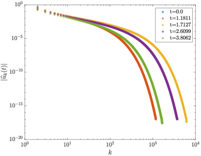
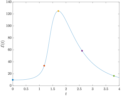
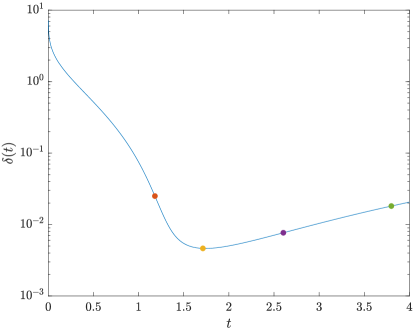
Figure 2: Solution of system (2) with $\alpha=0.6$ in (a) the physical space $u(t,x)$ and (b) the Fourier space $|\widehat{u}_{k}(t)|$ at the indicated time levels with the corresponding evolution of (c) the enstrophy $\mathcal{E}(t)$ and (d) the width of the analyticity strip $\delta(t)$. The symbols in panel (c) and (d) correspond to the time instances at which the solution is shown in panels (a) and (b).

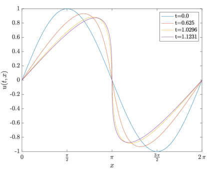
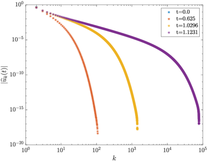
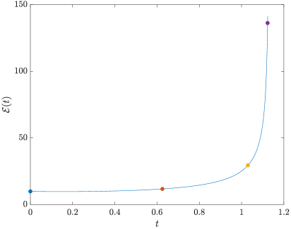
Figure 3: Solution of system (2) with $\alpha=0.4$ in (a) the physical space $u(t,x)$ and (b) the Fourier space $|\widehat{u}_{k}(t)|$ at the indicated time levels with the corresponding evolution of (c) the enstrophy $\mathcal{E}(t)$ and (d) the width of the analyticity strip $\delta(t)$. The symbols in panel (c) and (d) correspond to the time instances at which the solution is shown in panels (a) and (b).

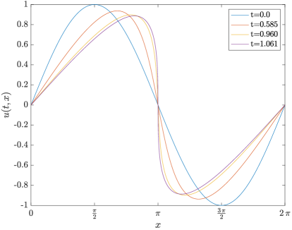
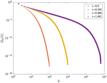
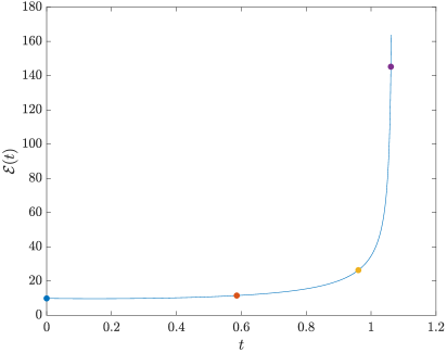
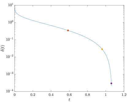
Figure 4: Solution of system (2) with $\alpha=0.1$ in (a) the physical space $u(t,x)$ and (b) the Fourier space $|\widehat{u}_{k}(t)|$ at the indicated time levels with the corresponding evolution of (c) the enstrophy $\mathcal{E}(t)$ and (d) the width of the analyticity strip $\delta(t)$. The symbols in panel (c) and (d) correspond to the time instances at which the solution is shown in panels (a) and (b).

Results obtained by solving system (2) with ${\alpha=0.6,0.4},0.1$ are presented in Figures 2, 3 and 4 where we show the solutions $u(t,x)$ in the physical space and in the spectral (Fourier) space at different time levels as well as the time evolution of the enstrophy ${\mathcal{E}}(t)$ and of the width of the analyticity strip $\delta(t)$. As regards the subcritical case with $\alpha=0.6$, in Figure 2a we see that around the time $t\approx 1.71$, the solution (marked with a yellow line) develops a steep front which is then smeared out by dissipation. This behaviour is also evident in the evolution of the Fourier spectrum $|\widehat{u}_{k}(t)|$ which at large times $t$ exhibits a faster decay with the wavenumber $k$, cf. Figure 2b. Since the solution remains smooth (analytic) throughout its entire evolution, the enstrophy ${\mathcal{E}}(t)$ and the width of the analyticity strip $\delta(t)$ remain bounded, respectively, from above and below. These quantities achieve their maximum and minimum values at the time when the front in the solution is the most steep, cf. Figures 2c–d.

In the supercritical cases with $\alpha=0.4$ and $\alpha=0.1$ presented in Figures 3 and 4 the computations are stopped at some point before the singularity occurs at $t=T^{*}$, which is caused by a rapid increase of the computational cost. In Figures 3a–b we see that at the singularity time the derivative of the solution at $x=\pi$ becomes unbounded, a blow-up mechanism which is also known from the inviscid Burgers problem (4) [31]. The singularity formation is also manifested by the enstrophy becoming unbounded and the width of the analyticity strip vanishing as $t\rightarrow(T^{*})^{-}$, cf. Figures 3c–d and 4c–d. As regards the Fourier spectra, in Figures 3b and 4b we observe that they extend to higher and higher wavenumbers as the blow-up time is approached and the region where the Fourier coefficients $\widehat{u}_{k}(t)$ decay exponentially fast with $k$ shrinks. This behavior marks the transition from an exponential to algebraic decay of the spectrum $|\widehat{u}_{k}(t)|$ with $k$ as the solution develops a singularity.

The time evolution of the enstrophy ${\mathcal{E}}(t)$ and of the width of the analyticity strip $\delta(t)$ are shown for several values of the exponent $\alpha$ in both the subcritical and supercritical regime in Figures 5a–b (the critical case with $\alpha=1/2$, where system (2) is known to be globally well-posed, cf. Theorem 2, is omitted due to its excessive computational cost). We see that as $\alpha\rightarrow(1/2)^{+}$ the maximum attained values of the enstrophy $\max_{t}{\mathcal{E}}(t)$ increase and the minimum attained values of the width of the analyticity strip $\min_{t}\delta(t)$ decrease. When $\alpha$ decreases to zero in the supercritical regime, blow-up occurs earlier as indicated by the instances of time when the enstrophy becomes unbounded and the width of the analyticity strip vanishes. In order to analyze this aspect quantitatively, in Figure 6a we show the blow-up times $T_{\mathcal{E}}^{*}(t)$ and $T_{\delta}^{*}(t)$ estimated using Algorithm 1 based on, respectively, the evolution of the enstrophy and of the width of the analyticity strip as functions of the location of the time window $I_{j}$ over which the optimization problem (23) is solved. These results are presented in Figure 6a for different supercritical values of $\alpha\in(0,1/2)$. We see that, interestingly, fits performed based on ${\mathcal{E}}(t)$ at early times underestimate the blow-up time while those performed based on $\delta(t)$ overestimate the blow-up time. However, as the windows $I_{j}$ approach the blow-up time, the two estimates $T_{\mathcal{E}}^{*}(t)$ and $T_{\delta}^{*}(t)$ agree with each other very well. In fact, the difference between these two estimates is $\mathcal{O}(10^{-3}-10^{-4})$ depending on $\alpha$, which allows us to conclude that the two approaches to estimating the blow-up time are consistent. Hereafter, we will estimate the blow-up time based on the evolution of the enstrophy as this approach can also be used in the stochastic case (since solutions of the stochastic problem (12) are not in general analytic functions of the space coordinate, we have $\delta(t)=0$, $\forall t>0$ in this case). We will therefore set $T^{*}=T^{*}_{\mathcal{E}}(t_{K})$.

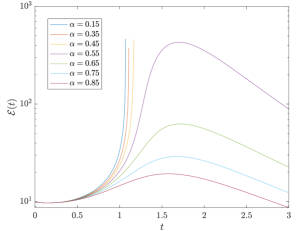
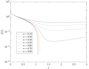
Figure 5: Time evolution of (a) the enstrophy ${\mathcal{E}}(t)$ and (b) the width of the analyticity strip $\delta(t)$ in solutions of the fractional Burgers equation (2) with different indicated values of the fractional dissipation exponent $\alpha$.

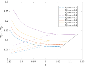
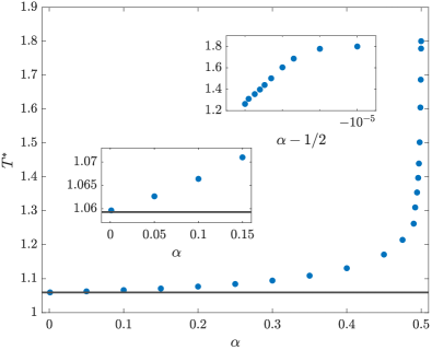
Figure 6: (a) Estimates of the blow-up time based on the enstrophy $T^{*}_{\mathcal{E}}$ (dashed lines) and on the width of the analyticity strip $T^{*}_{\delta}$ (solid lines) as functions of time for different values of $\alpha$. The time $t$ is understood here as the position of the center of the window $I_{j}$, $j=1,\dots,K$, over which fits are performed when solving optimization problem (23), cf. Algorithm 1. Curves with the same color indicate the estimates obtained for the same value of $\alpha$. The black slanted line corresponds to $T^{*}=t$ and serves as a reference for how far the estimate of $T^{*}$ can be continued. (b) Dependence the estimated blow-up times $T^{*}$ on the fractional dissipation exponent $\alpha$. The top and bottom inset represent small neighborhoods near the endpoints $\alpha=1/2$ and $\alpha=0$, whereas the horizontal line denotes the blow up time $T^{*}_{1}$ in the limiting case when $\alpha\rightarrow 0^{+}$, cf. (7).

The blow-up times $T^{*}$ determined as discussed above are shown as functions of $\alpha\in(0,1/2)$ in Figure 6b. We remark that in order to explore behaviors corresponding to the limiting values of this parameter, its smallest and largest values are, respectively, $\alpha=10^{-3}$ and $\alpha=1/2-10^{-5}$. As is evident from Figure 6b, the blow-up time $T^{*}$ is an increasing function of $\alpha$. In the limit $\alpha\rightarrow 0$ it tends to the value given by expression (7) for the limiting system (6). The data in Figure 6b also suggests that the blow-up time $T^{*}$ remains bounded in the opposite limit when $\alpha\rightarrow(1/2)^{-}$.

Finally, we consider the behavior of the blow-up time $T^{*}$ in the inviscid limit $\nu\rightarrow 0$ with fixed $\alpha\in(0,1/2)$. The results shown in Figure 7 demonstrate that as $\nu$ vanishes the blow-up time $T^{*}$ approaches the blow-up time for the inviscid problem (4), cf. expression (5), uniformly in $\alpha$. In this figure we also observe that the relative range of variation of $T^{*}$ is reduced as $\nu$ decreases. Some additional details concerning the results presented in this section are available in [36]. In the next section we discuss how the behavior of fractional Burgers flows is affected by the stochastic forcing introduced in Section 2.2.

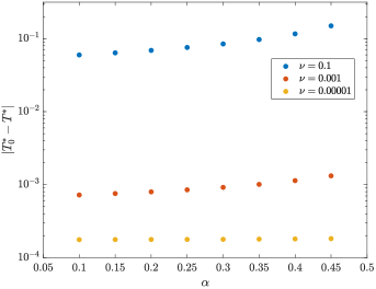
Figure 7: The difference between the blow-up times $T^{*}$ characterizing solutions of the fractional Burgers system (2) with given $\alpha$ and $\nu$ and the blow-up time $T_{0}^{*}=1$ in the solution of the inviscid problem (4), which is independent of $\alpha$, cf. (5).

5 Results — Stochastic Case

In this section we present results obtained for the stochastic fractional Burgers system (12), first in the supercritical regime (with $\alpha=0.4$) and then in the subcritical regime (with $\alpha=0.6$). We use the same initial condition and same value of the viscosity coefficient as in the deterministic case, i.e., $g(x)=\sin(x)$ and $\nu=0.11$. The problem is solved using the approach described in Section 3.2 with the spatial resolution given by $N=2^{17}=131,072$ and $N=2^{15}=32,768$ in the supercritical and subcritical regimes, respectively. The number of Monte-Carlo samples $M$ used to discretize the probability space will be specified individually in the different cases below.

5.1 Supercritical Regime

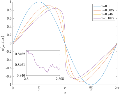
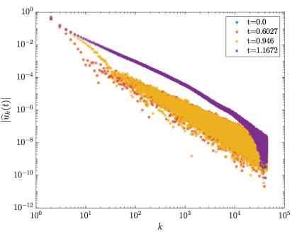
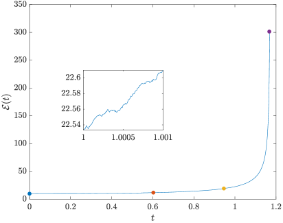
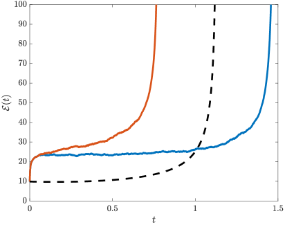
Figure 8: A single stochastic realization of the solution of system (12) with $\alpha=0.4$ and $\rho=10^{-2}$ in (a) the physical space $u(t,x)$ and (b) the Fourier space $|\widehat{u}_{k}(t)|$ at the indicated time levels with the corresponding evolution of the enstrophy $\mathcal{E}(t)$ in panel (c). The symbols in panel (c) correspond to the time instances at which the solution is shown in panels (a) and (b). (d) Time evolution of the enstrophy in the stochastic realizations of the solution of system (12) with $\alpha=0.4$ and $\rho=5\cdot 10^{-2}$ with blow-up occurring at the shortest and latest recorded times $T^{*}$ (solid lines), and in the solution of the deterministic problem (2) with the same value of $\alpha$ (dashed line).

As regards the supercritical regime, the main question we want to address is the effect of the stochastic excitation on the blow-up time $T^{*}$ and to this end we have solved system (12) with $\alpha=0.4$ and with different noise amplitudes $\rho=10^{-6},10^{-4},10^{-2},2\cdot 10^{-2},5\cdot 10^{-2}$, in each case using $M=2\cdot 10^{4}$ Monte Carlo samples. The time evolution of a representative stochastic realization of the solution with an intermediate noise level $\rho=10^{-2}$ is shown in Figures 8a and 8b in the physical and Fourier space, respectively. Comparing these results with Figures 3a,b corresponding to the deterministic case, we observe that the large-scale features of the solution remain unaffected and the effect of noise is to produce small-scale oscillations. As is evident from Figure 8b, the Fourier spectrum of the solution no longer decays exponentially fast for large wavenumbers. The corresponding time evolution of the enstrophy shown in Figures 8c indicates that its growth is now non-monotonic. Different stochastic realizations with a given value of $\rho$ exhibit singularity formation at times $T^{*}$ which can be both shorter and longer than the blow-up time in the deterministic case. However, in none of these cases did we find any evidence for noise to regularize solutions, so that blow-up would not occur in finite time at all. To illustrate this point, in Figures 8d we show the enstrophy evolutions in the stochastic realizations corresponding to the singularity occurring at the earliest and latest recorded times $T^{*}$ when the noise amplitude is $\rho=5\cdot 10^{-2}$. It is clear from this figure that noise may nonetheless significantly accelerate or delay singularity formation.

The blow-up time $T^{*}$, estimated here using Algorithm 1, is a random variable and we now go on to analyze its statistical properties. Probability density functions (PDFs) of $T^{*}$ are shown in Figures 9a–d for four different values of the noise amplitude $\rho$. We see that while for small noise magnitudes the PDFs of the blow-up time have distributions close to the Gaussian distribution, for increasing $\rho$ they develop “heavy” tails and become skewed towards longer times. Interestingly, this increasing non-Gaussianity of the distributions is accompanied by the mean value of $T^{*}$ shifting towards shorter times while its standard deviation increases. This means that as the noise amplitude $\rho$ increases, blow-up on average occurs earlier than in the deterministic case, however, realizations in which blow-up is significantly delayed also become more likely.

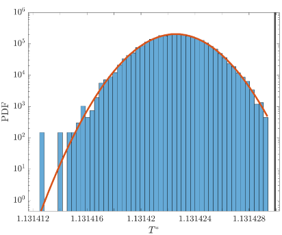
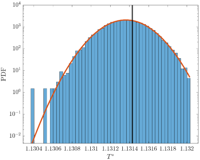
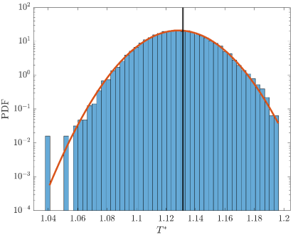
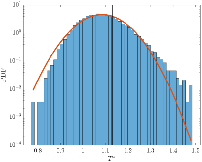
Figure 9: PDFs of the blow-up time $T^{*}$ in solutions of the stochastic problem (12) with different noise amplitudes (a) $\rho=10^{-6}$ , (b) $\rho=10^{-4}$, (c) $\rho=10^{-2}$ and (d) $\rho=5\cdot 10^{-2}$. Red curves represent the Gaussian distributions with the same means and standard deviations, whereas black vertical lines denote the blow-up times in the deterministic case.

In order to quantify the observations made above, we compute the first four statistical moments, namely the mean $\mu:={\mathbb{E}}[T^{*}]$, standard deviation $\sigma:={\mathbb{E}}[(T^{*}-\mu)^{2}]$, skewness ${\mathcal{S}}:={\mathbb{E}}\left[\left((T^{*}-\mu)/\sigma\right)^{3}\right]$ and kurtosis ${\mathcal{K}}:={\mathbb{E}}\left[\left((X-\mu)/\sigma\right)^{4}\right]$, where ${\mathbb{E}}[\cdot]$ is the expected value, of the blow-up times obtained for different noise amplitudes $\rho$. These moments are approximated as follows

$$\mu \approx \mu_{m} :=\frac{1}{m}\sum_{j=1}^{m}T_{j}^{*},$$ (24a)

$$\sigma \approx \sigma_{m} :=\frac{1}{m}\sum_{j=1}^{m}(T_{j}^{*}-\mu_{m})^{2},$$ (24b)

$${\mathcal{S}} \approx {\mathcal{S}}_{m} :=\frac{1}{m}\sum_{j=1}^{m}\left(\frac{T_{j}^{*}-\mu_{m}}{\sigma_{m}}\right)^{3},$$ (24c)

$${\mathcal{K}} \approx {\mathcal{K}}_{m} :=\frac{1}{m}\sum_{j=1}^{m}\left(\frac{T_{j}^{*}-\mu_{m}}{\sigma_{m}}\right)^{4},$$ (24d)

where $m=1,\dots,M$ is the number of samples used to construct the approximations and $\{T_{j}^{*}\}_{j=1}^{M}$ are the blow-up times in the realizations from the Monte-Carlo ensemble. It is known that moments of increasing order are harder to approximate accurately via relations (24) for random variables characterized by PDFs with heavy tails, such as the PDF shown in Figure 9d. In order to estimate how many samples are required to accurately estimate the moments for different values of the noise amplitude $\rho$, in Figures 10a,c and 11a,c we show the estimates $\mu_{m}$, $\sigma_{m}$, ${\mathcal{S}}_{m}$ and ${\mathcal{K}}_{m}$ for $m=1,\dots,M$. These results indicate how the estimated moments depend on the number of samples $m$ used in the calculation. They are complemented by plots of the relative errors defined as

$$e^{X}_{m}:=\left|\frac{X_{m}-X_{M}}{X_{M}}\right|,\qquad m=1,\dots,M,\quad X=\mu,\sigma,{\mathcal{S}},{\mathcal{K}},$$ (25)

where the estimates $X_{M}$ computed based on all available $M$ samples are used as the “true” values, shown in Figures 10b,d and 11b,d. We see in these last plots that the relative errors decrease in proportion to $m^{-1/2}$, as expected for a Monte-Carlo approximation. Overall, in Figures 10a–d and 11a–d we observe that approximation errors are larger for moments of higher order and they also increase with the noise magnitude $\rho$ as the PDFs become increasingly non-Gaussian, cf. Figure 9. However, we can conclude that the total number of Monte-Carlo samples $M=2\cdot 10^{4}$ is sufficient to ensure required accuracy in all cases. On the other hand, the trends evident in Figures 10a–d and 11a–d indicate that a significantly larger number of Monte-Carlo samples would be required to obtain converged statistics for a higher value of $\rho$, which was not attempted due to a prohibitive computational cost.

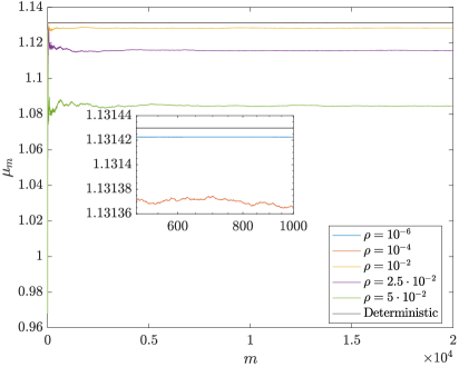
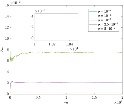
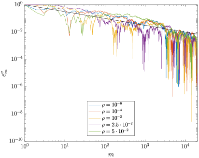
Figure 10: Approximations (a) $\mu_{m}$ of the mean and (c) $\sigma_{m}$ of the standard deviation together with their relative errors (b) $e^{\mu}_{m}$ and (d) $e^{\sigma}_{m}$ as functions of the number of samples $m$ used in the computation. The straight black line in panels (b) and (d) represents the expression $m^{-1/2}$.

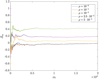
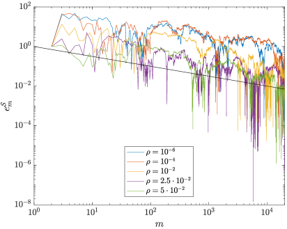
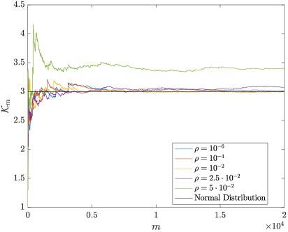
Figure 11: Approximations (a) ${\mathcal{S}}_{m}$ of the skewness and (c) ${\mathcal{K}}_{m}$ of the kurtosis together with their relative errors (b) $e^{{\mathcal{S}}}_{m}$ and (d) $e^{{\mathcal{K}}}_{m}$ as functions of the number of samples $m$ used in the computation. The straight black line in panels (b) and (d) represents the expression $m^{-1/2}$.

Finally, the mean blow-up time, its standard deviation, skewness and kurtosis, which were estimated using relations (24a)–(24d), are shown as functions of $\rho$ in Figures 12a–d. The plots also involve error bars computed using the bootstrapping method [22, 18] assuming 95% confidence which reflect the approximation errors due to finite numbers of Monte-Carlo samples, cf. Figures 10 and 11. Figures 12a and 12b show that over the considered range of $\rho$ the mean blow-up time decreases with noise amplitude whereas its standard deviation grows. Figures 12c and 12d show that skewness and kurtosis also grow as $\rho$ becomes large providing evidence for an increasing non-Gaussianity of the distribution of blow-up times. In order to quantify these trends, Figures 12a–d include fits constructed using the power-law relation

$$f(\rho):=a\,\rho^{b}+c,\qquad a,b,c\in{\mathbb{R}},$$ (26)

with the obtained parameters reported in Table 1 (we set $c=0$ in the fits to the mean blow-up time and its variance). One can see that while the dependence of the variance, skewness and kurtosis on $\rho$ is well-represented by relation (26), this is not the case for the mean blow-up time. However, for each statistical moment the optimal power-law relation involves a different exponent $b$.

Statistical Moment	a	b	c
$\mu_{M}$	0.233	0.792	0
$\rho_{M}$	3.136	1.984	0
$\mathcal{S}_{M}$	12.888	1.128	-0.015
$\mathcal{K}_{M}$	1008.425	2.615	3

Table 1: Parameters of the fits to the data shown in Figures 12a–d using the power-law relation (26).

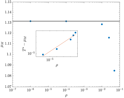
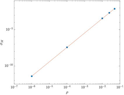
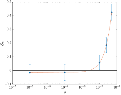
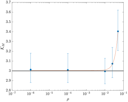
Figure 12: Estimated (a) mean blow time $T^{*}$, (b) its standard deviation, (d) skewness and (e) kurtosis as functions of the noise amplitude $\rho$. The horizontal line in (a) corresponds to the blow-up time in the deterministic case, whereas the horizontal lines in (c) and (d) represent the values characterizing the Gaussian distribution, The red curves correspond to the fits obtained using the power-law relation (26) with the parameters reported in Table 1.

5.2 Subcritical Regime

We now go on to analyze the results obtained for the subcritical case with $\alpha=0.6$ and with different noise amplitudes $\rho=10^{-6},10^{-4},10^{-2},5\cdot 10^{-2},10^{-1}$. In each case we use $M=1.2\cdot 10^{4}$ Monte-Carlo samples which was found to be a sufficient number based on an analysis similar to that reported in Figures 10–11. Since no evidence was found for noise-induced blow-up in the subcritical case, the key question is about the effect of noise of on the maximum attained enstrophy ${\mathcal{E}^{\rho}_{\text{max}}}:=\max_{t\geq 0}{\mathcal{E}}(t)$ and on the time when this maximum occurs ${T^{\rho}_{\text{max}}}:=\operatorname{argmax}_{t\geq 0}{\mathcal{E}}(t)$.

We begin by comparing the time evolution of the enstrophy in the stochastic realizations with the largest and smallest values of ${\mathcal{E}^{\rho}_{\text{max}}}$ obtained for $\rho=10^{-2}$ and $\rho=5\cdot 10^{-2}$ in Figures 13a and 13b, respectively, where we also show the evolution of the enstrophy in the deterministic case. We observe that when the maximum enstrophy achieved in a stochastic realization is higher than in the deterministic case, the maximum tends to occur at an earlier time, and vice versa. By comparing Figures 13a and 13b we also note that the spread between the largest and smallest values of ${\mathcal{E}^{\rho}_{\text{max}}}$ increases with the noise magnitude $\rho$. In Figure 13c we show the dependence of the expected value of the enstrophy ${\mathbb{E}}[{\mathcal{E}}(u(t))]$ of the stochastic solution on time $t$. We see that as $\rho$ increases then so do the expected values of the enstrophy ${\mathbb{E}}[{\mathcal{E}}(u(t))]$ at any fixed time $t\in[0,T]$ and their maxima occur at earlier times.

We remark that one might be tempted to also consider the enstrophy of the expected values of the solution ${\mathcal{E}}({\mathbb{E}}[u(t)])$. However, these two quantities (and their estimates of the type (24a)) are related via Jensen’s inequality [32, 35]

$${\mathbb{E}}[{\mathcal{E}}(u(t))]\geq{\mathcal{E}}({\mathbb{E}}[u(t)]),\qquad\forall t,$$ (27)

and therefore we will exclusively focus here on the former quantity.

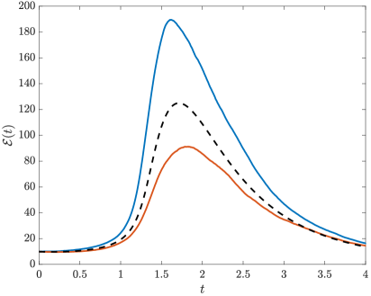
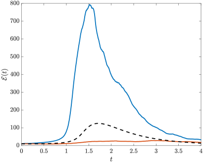
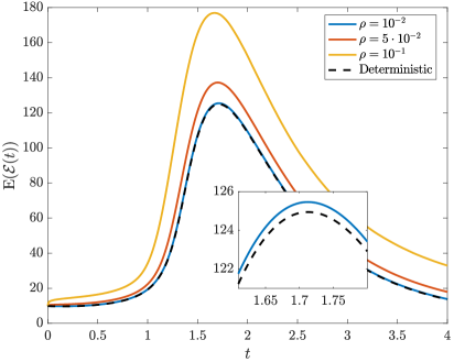
Figure 13: Solid lines in (a) and (b) represent the time evolutions of the enstrophy ${\mathcal{E}}(t)$ in the stochastic realizations characterized by the largest and smallest values of ${\mathcal{E}^{\rho}_{\text{max}}}$ for (a) $\rho=10^{-2}$ and (b) $\rho=5\cdot 10^{-2}$. The dashed line in (a) and (b) corresponds to the deterministic case. Panel (c) shows the time evolution of the expected value of the enstrophy ${\mathbb{E}}[{\mathcal{E}}(u(t))]$ of the stochastic solution for the three largest values of $\rho=10^{-2},5\cdot 10^{-2},10^{-1}$.

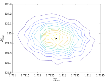
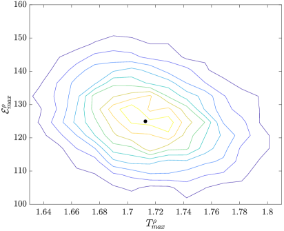
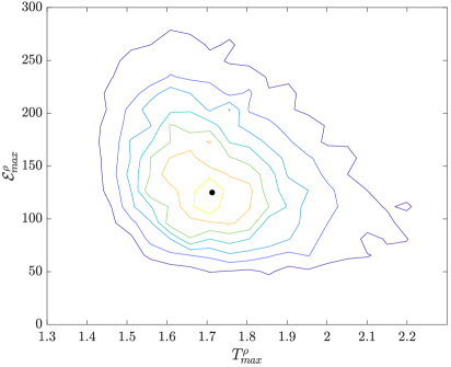
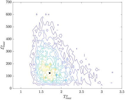
Figure 14: Equispaced level sets of the JPDFs of ${T^{\rho}_{\text{max}}}$ and ${\mathcal{E}^{\rho}_{\text{max}}}$ for the noise amplitudes (a) $\rho=10^{-4}$, (b) $\rho=10^{-2}$, (c) $\rho=5\times 10^{-2}$ and (d) $\rho=10^{-1}$. Yellow level sets correspond to large values of the JPDF, whereas black symbols represent the values of $T_{\text{max}}$ and ${\mathcal{E}}_{\text{max}}$ in the deterministic case.

In order to elucidate the correlation between the values of ${\mathcal{E}^{\rho}_{\text{max}}}$ and ${T^{\rho}_{\text{max}}}$ in different stochastic realizations, joint probability density functions (JPDFs) of these quantities are shown in Figures 14a–d for different values of $\rho$. We see that as the noise amplitude grows, larger values of ${\mathcal{E}^{\rho}_{\text{max}}}$ become increasingly correlated with times ${T^{\rho}_{\text{max}}}$ shorter than in the deterministic case. By the same token, reduced values of ${\mathcal{E}^{\rho}_{\text{max}}}$ become increasingly correlated with times ${T^{\rho}_{\text{max}}}$ longer than in the deterministic case. Interestingly, for larger values of $\rho$ there is a well-defined minimum time ${T^{\rho}_{\text{max}}}$, which depends on $\rho$, such that maximum values of enstrophy are unlikely to be obtained before that time. We also add that we compute our stochastic realizations over a fixed time window $[0,T]$ with $T=4$. Therefore, as $\rho$ grows and large values of ${T^{\rho}_{\text{max}}}\lessapprox 4$ become more likely, it becomes increasingly difficult to capture enstrophy maxima as they begin to occur near the end of the considered time window.

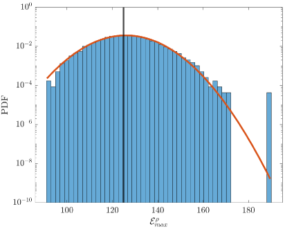
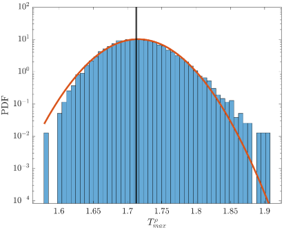
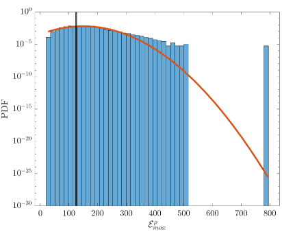
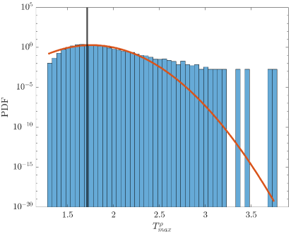
Figure 15: PDFs of (a,c) the maximum attained enstrophy ${\mathcal{E}^{\rho}_{\text{max}}}$ and (b,d) the time ${T^{\rho}_{\text{max}}}$ when the maximum occurs in solutions of the stochastic problem (12) with different noise amplitudes (a,b) $\rho=10^{-2}$ and (c,d) $\rho=5\cdot 10^{-2}$. Red curves represent the Gaussian distributions with the same means and standard deviations, whereas black vertical lines denote the values of $T_{\text{max}}$ in the deterministic case.

In order to shed further light on the trends observed in Figures 14a–d, the PDFs of ${\mathcal{E}^{\rho}_{\text{max}}}$ and ${T^{\rho}_{\text{max}}}$ for two selected values of $\rho$ are shown in Figures 15a–b. It is evident that as the noise amplitude becomes larger, the PDFs of both ${\mathcal{E}^{\rho}_{\text{max}}}$ and ${T^{\rho}_{\text{max}}}$ become increasingly non-Gaussian, with this trend appearing more pronounced in the case of ${T^{\rho}_{\text{max}}}$. In particular, the PDFs become strongly skewed with heavy tails towards large values of ${\mathcal{E}^{\rho}_{\text{max}}}$ and ${T^{\rho}_{\text{max}}}$. On the other hand, values of these quantities significantly smaller than in the deterministic case are much less likely to occur. To analyze these trends in quantitative terms, the four first statistical moments of the distributions of ${\mathcal{E}^{\rho}_{\text{max}}}$ and ${T^{\rho}_{\text{max}}}$, defined analogously to (24a)–(24d), are plotted in Figures 16 and 17 as functions of the noise amplitude $\rho$. We remark that the dependence of the estimates of these moments on the number of samples used in their evaluation is similar to what was shown in Figures 10–11, and these results are omitted here for brevity.

In Figures 16a we see that the mean value of ${\mathcal{E}^{\rho}_{\text{max}}}$ increases with $\rho$ which is consistent with the trend observed in Figure 13c for the expected value of the enstrophy ${\mathbb{E}}[{\mathcal{E}}(u(t))]$, although the mean values of ${\mathcal{E}^{\rho}_{\text{max}}}$ exceed the values of $\max_{t>0}{\mathbb{E}}[{\mathcal{E}}(u(t))]$ for all $\rho$. On the other hand, in Figures 17a we see that the mean time ${T^{\rho}_{\text{max}}}$ when the maximum enstrophy is attained also increases with $\rho$ which should be contrasted with Figure 13c showing that the maxima of the expected value of the enstrophy ${\mathbb{E}}[{\mathcal{E}}(u(t))]$ occur at earlier times as the noise amplitude increases. The reason for this somewhat surprising effect is that the operation of computing the maximum of a function, or the argument corresponding to the maximum, is not linear and hence does not commute with the operation of computing the average.

In order to quantify the dependence of the statistical moments of ${\mathcal{E}^{\rho}_{\text{max}}}$ and ${T^{\rho}_{\text{max}}}$ on the noise magnitude $\rho$, Figures 16a–d and 17a–d also include fits obtained using the power-law relation (26) with parameters reported in Tables 3 and 3. As was the case for the moments of the blow-up time in the supercritical regime, cf. Figure 12, we see that while the dependence of the variance, skewness and kurtosis of the distributions of ${\mathcal{E}^{\rho}_{\text{max}}}$ and ${T^{\rho}_{\text{max}}}$ on $\rho$ is represented rather well by relation (26), this is not the case for the mean values of ${\mathcal{E}^{\rho}_{\text{max}}}$ and ${T^{\rho}_{\text{max}}}$. Interestingly, the values of the exponent $b$ describing the dependence of the variance, skewness and kurtosis of the distributions of ${\mathcal{E}^{\rho}_{\text{max}}}$ on $\rho$, cf. Table 3, are similar to those reported in Table 1 for the blow-up time in the supercritical regime. Other than this, there seems to be no obvious pattern in how the different statistical moments depend on the noise amplitude $\rho$.

Statistical Moment	a	b	c
$\mu_{M}$	175.027	1.42	0
$\sigma_{M}$	$2.18\cdot 10^{6}$	2.05	0
$\mathcal{S}_{M}$	21.33	1.13	-0.041
$\mathcal{K}_{M}$	868.48	1.95	2.99

Table 2: Parameters of the fits to the data shown in Figures 16a–d using the power-law relation (26).

Statistical Moment	a	b	c
$\mu_{M}$	0.62	1.03	0
$\sigma_{M}$	8.307	1.73	0
$\mathcal{S}_{M}$	13.07	0.74	-0.035
$\mathcal{K}_{M}$	40.72	0.72	2.62

Table 3: Parameters of the fits to the data shown in Figures 17a–d using the power-law relation (26).

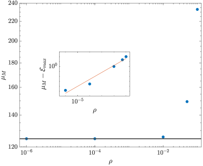
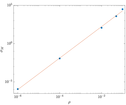
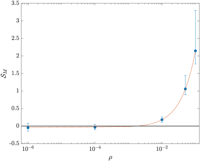
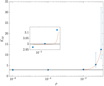
Figure 16: Estimated (a) mean maximum enstrophy ${\mathcal{E}^{\rho}_{\text{max}}}$, (b) its standard deviation, (c) skewness and (d) kurtosis as functions of the noise amplitude $\rho$. The horizontal line in (a) corresponds to the maximum enstrophy in the deterministic case, whereas the horizontal lines in (c) and (d) represent the values characterizing the Gaussian distribution. The red curves correspond to the fits obtained using the power-law relation (26) with the parameters reported in Table 3.

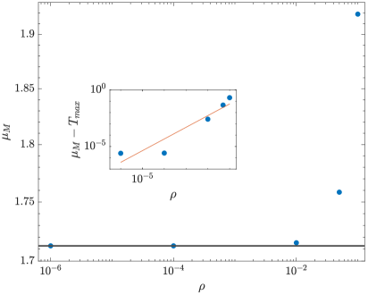
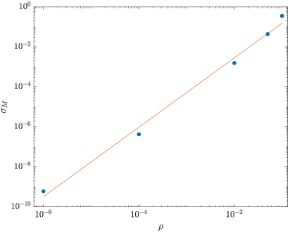
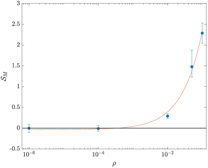
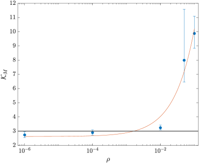
Figure 17: Estimated (a) mean time ${T^{\rho}_{\text{max}}}$ when the maximum enstrophy is attained, (b) its standard deviation, (c) skewness and (d) kurtosis as functions of the noise amplitude $\rho$. The horizontal line in (a) corresponds to the time where the maximum enstrophy is attained in the deterministic case, whereas the horizontal lines in (c) and (d) represent the values characterizing the Gaussian distribution. The red curves correspond to the fits obtained using the power-law relation (26) with the parameters reported in Table 3.

6 Summary and Conclusions

This study is motivated by the question of how singularity formation and other forms of extreme behavior in nonlinear dissipative partial differential equations are affected by stochastic excitations [24]. As a model problem, we have considered the 1D fractional Burgers equation (2) with additive colored noise. This system is interesting, because in the deterministic setting it exhibits finite-time blow-up or a globally well-posed behavior depending on the value of the fractional dissipation exponent $\alpha$. The question we are interested in is addressed by performing a series of very accurate numerical computations combining spectrally-accurate spatial discretizations with a Monte-Carlo approach where convergence of all approximations was checked very carefully. It should be emphasized that even though the problem is formulated in 1D, these computations are in fact quite challenging since resolving an emerging singularity requires refined numerical resolutions both in space and in time, and this difficulty is compounded by a slow convergence of the Monte-Carlo approach.

As the first main contribution, we carefully documented the singularity formation in the deterministic system in the supercritical regime. It was shown that for a fixed initial condition the blow-up time $T^{*}$ is a decreasing function of the fractional dissipation exponent $\alpha\in[0,1/2)$ and tends to the expected limiting values as $\alpha\rightarrow 0$ and $\nu\rightarrow 0$, cf. Figures 6b and 7. When $\alpha\rightarrow(1/2)^{-}$ the blow-up time approaches a finite value.

Our second main finding is that while there is no evidence for noise to prevent singularity formation in the supercritical regime, the distribution of the blow-up times $T^{*}$ (understood as a stochastic variable) becomes increasingly non-Gaussian as the noise amplitude $\rho$ increases, cf. Figure 9. Interestingly, as $\rho$ grows, the mean blow-up time is reduced but at the same time significantly delayed blow-up times also become more likely. This is because the PDFs of $T^{*}$ become more skewed and develop heavy tails towards large blow-up times as $\rho$ increases. These observations are complemented by our findings for the subcritical case where we noted that the expected value of the enstrophy ${\mathbb{E}}[{\mathcal{E}}(t)]$ of the stochastic solution at any fixed time $t$ increases with the noise magnitude $\rho$ (Figure 13c). Interestingly, while its maxima are attained at earlier times as compared to the deterministic case, the mean time when the enstrophy maxima are attained in individual stochastic realizations is in fact larger than in the deterministic case and increases with $\rho$, cf. Figure 17a. Increasingly non-Gaussian behavior of the PDFs of ${\mathcal{E}^{\rho}_{\text{max}}}$ and ${T^{\rho}_{\text{max}}}$ is evident as $\rho$ becomes large in the subcritical case we well (Figures 15a–d).

To conclude, as is evident from the discussion above, the answer to the question about the effect of stochastic excitations on extreme and singular behavior in fractional Burgers flows is rather nuanced. It is clear, however, that there is no evidence for the noise to regularize the evolution by suppressing blow-up in the supercritical regime, or for the noise to trigger blow-up in the subcritical regime. It has to be recognized that due to the computational cost the results reported here are restricted to small and intermediate noise magnitudes only. Whether or not the trends reported in this study will hold also for much larger noise amplitudes is an interesting open question.

References

- [1] R. A. Adams and J. F. Fournier. Sobolev Spaces. Elsevier, 2005.
- [2] Sergio Albeverio and Olga Rozanova. The non-viscous Burgers equation associated with random position in coordinate space: a threshold for blow up behaviour. Mathematical Models and Methods in Applied Sciences, 19(05):749–767, 2009.
- [3] Sergio Albeverio and Olga Rozanova. Suppression of unbounded gradients in an SDE associated with the Burgers equation. Proceedings of the American Mathematical Society, 138(1):241–251, 2010.
- [4] N. Alibaud, J. Droniou, and J. Vovelle. Occurrence and non-appearance of shocks in fractal Burgers equations. J. Hyperbolic Differ. Equ., 4:479–499, 2007.
- [5] D. Ayala and B. Protas. On maximum enstrophy growth in a hydrodynamic system. Physica D, 240:1553–1563, 2011.
- [6] E. Balkovsky, G. Falkovich, I. Kolokolov, and V. Lebedev. Intermittency of Burgers’ Turbulence. Phys. Rev. Lett., 78:1452–1455, Feb 1997.
- [7] Jérémie Bec and Konstantin Khanin. Burgers turbulence. Physics Reports, 447(1–2):1–66, 2007.
- [8] T. R. Bewley. Numerical Renaissance. Renaissance Press, 2009.
- [9] Alexandre Boritchev. Decaying turbulence in the generalised Burgers equation. Archive for Rational Mechanics and Analysis, 214(1):331–357, 2014.
- [10] J. P. Boyd. Chebyshev and Fourier Spectral Methods. Dover, 2001.
- [11] M. D. Bustamante and M. Brachet. Interplay between the Beale-Kato-Majda theorem and the analyticity-strip method to investigate numerically the incompressible Euler singularity problem. Phys. Rev. E, 86:066302, 2012.
- [12] M. D. Bustamante and R. M. Kerr. 3D Euler about a 2D symmetry plane. Physica D, 237:1912–1920, 2008.
- [13] C. Canuto, A. Quarteroni, Y. Hussaini, and T. A. Zang. Spectral Methods. Scientific Computation. Springer, 2006.
- [14] C. H. Chan, M. Czubak, and L. Silvestre. Eventual Regularization of The Slightly Supercritical Fractional Burgers Equation. Discrete and Continuous Dynamical Systems A, 27:847–861, 2010.
- [15] C. Chang. Numerical solution of stochastic differential equations with constant diffusion coefficients. Mathematics of Computation, 49(180):523–542, 1987.
- [16] Alexei Chekhlov and Victor Yakhot. Kolmogorov turbulence in a random-force-driven Burgers equation. Phys. Rev. E, 51:R2739–R2742, Apr 1995.
- [17] Alexei Chekhlov and Victor Yakhot. Kolmogorov turbulence in a random-force-driven Burgers equation: Anomalous scaling and probability density functions. Phys. Rev. E, 52:5681–5684, Nov 1995.
- [18] A. C. Davison and D. V. Hinkley. Bootstrap Methods and Their Applications. Cambridge University Press, 1997.
- [19] A. Debussche and L. Di Menza. Numerical simulation of focusing stochastic nonlinear Schrödinger equations. Physica D, 162:131–154, 2002.
- [20] C. R. Doering. The 3D Navier-Stokes problem. Annual Review of Fluid Mechanics, 41:109–128, 2009.
- [21] H. J. Dong, D. P. Du, and D. Li. Finite time singularities and global well-posedness for fractal Burgers equations. Indiana Univ. Math. J., 58:807–821, 2009.
- [22] B. Efron and T. DiCiccio. Bootstrap confidence intervals. Statistical Science, 11(3):89–228, 1996.
- [23] C. L. Fefferman. Existence and smoothness of the Navier-Stokes equation. available at http://www.claymath.org/sites/default/files/navierstokes.pdf, 2000. Clay Millennium Prize Problem Description.
- [24] Franco Flandoli. Random Perturbation of PDEs and Fluid Dynamic Models. Lecture Notes in Mathematics. Springer, 2015.
- [25] Franco Flandoli. Stochastic Analysis: A Series of Lectures (Eds. R.C. Dalang, M. Dozzi, F. Flandoli and F. Russo), chapter A Stochastic View over the Open Problem of Well-posedness for the 3D Navier-Stokes Equations, pages 221–246. Birkhäuser, 2015.
- [26] Toshiyuki Gotoh and Robert H. Kraichnan. Statistics of decaying Burgers turbulence. Physics of Fluids A, 5(2):445–457, 1993.
- [27] Tobias Grafke, Rainer Grauer, and Tobias Schäfer. The instanton method and its numerical implementation in fluid mechanics. Journal of Physics A: Mathematical and Theoretical, 48(33):333001, 2015.
- [28] N.H. Katz and N. Pavlović. A cheap Caffarelli-Kohn-Nirenberg inequality for the Navier-Stokes equation with hyper-dissipation. Geometric & Functional Analysis GAFA, 12(2):355–379, 2002.
- [29] A. Kiselev, F. Nazaraov, and R. Shterenberg. Blow up and regularity for fractal Burgers equation. Dynamics of Partial Differential Equations, 5:211–240, 2008.
- [30] Christian Klein and Jean-Claude Saut. A numerical approach to blow-up issues for dispersive perturbations of Burgers’ equation. Physica D, 295–296:46–65, 2015.
- [31] H. Kreiss and J. Lorenz. Initial-Boundary Value Problems and the Navier-Stokes Equations, volume 47 of Classics in Applied Mathematics. SIAM, 2004.
- [32] Gabriel J. Lord, Catherine E. Powell, and Tony Shardlow. An Introduction to Computational Stochastic PDEs. Cambridge University Press, 2014.
- [33] Baruch Meerson, Eytan Katzav, and Arkady Vilenkin. Large deviations of surface height in the Kardar-Parisi-Zhang equation. Phys. Rev. Lett., 116:070601, Feb 2016.
- [34] J. Nocedal and S. J. Wright. Numerical Optimization. Springer, 1999.
- [35] Diogo Poças and Bartosz Protas. Transient growth in stochastic Burgers flows. Discrete & Continuous Dynamical Systems — B, 23:2371, 2018.
- [36] E. Ramírez. Singularity formation in the deterministic and stochastic fractional burgers equations. Master’s thesis, McMaster University, 2020.
- [37] James C Robinson. The Navier-Stokes regularity problem. Phil. Trans. R. Soc. A, 378:20190526, 2020.
- [38] Zhen-Su She, Erik Aurell, and Uriel Frisch. The inviscid Burgers equation with initial data of brownian type. Communications in Mathematical Physics, 148(3):623–641, 1992.
- [39] Ya. G. Sinai. Statistics of shocks in solutions of inviscid Burgers equation. Communications in Mathematical Physics, 148(3):601–621, 1992.
- [40] C. Sulem, P. L. Sulem, and H. Frisch. Tracing complex singularities with spectral methods. Journal of Computational Physics, 50:138–161, 1983.
- [41] Dongfang Yun and Bartosz Protas. Maximum Rate of Growth of Enstrophy in Solutions of the Fractional Burgers Equation. Journal of Nonlinear Science, 28(1):395–422, Feb 2018.
- [42] Oleg Zikanov, Andre Thess, and Rainer Grauer. Statistics of turbulence in a generalized random-force-driven Burgers equation. Physics of Fluids, 9(5):1362–1367, 1997.