Adaptive learning for financial markets
mixing model-based and model-free RL for volatility targeting

Abstract.

Model-Free Reinforcement Learning has achieved meaningful results in stable environments but, to this day, it remains problematic in regime changing environments like financial markets. In contrast, model-based RL is able to capture some fundamental and dynamical concepts of the environment but suffer from cognitive bias. In this work, we propose to combine the best of the two techniques by selecting various model-based approaches thanks to Model-Free Deep Reinforcement Learning. Using not only past performance and volatility, we include additional contextual information such as macro and risk appetite signals to account for implicit regime changes. We also adapt traditional RL methods to real-life situations by considering only past data for the training sets. Hence, we cannot use future information in our training data set as implied by K-fold cross validation. Building on traditional statistical methods, we use the traditional ”walk-forward analysis”, which is defined by successive training and testing based on expanding periods, to assert the robustness of the resulting agent.

Finally, we present the concept of statistical difference’s significance based on a two-tailed T-test, to highlight the ways in which our models differ from more traditional ones. Our experimental results show that our approach outperforms traditional financial baseline portfolio models such as the Markowitz model in almost all evaluation metrics commonly used in financial mathematics, namely net performance, Sharpe and Sortino ratios, maximum drawdown, maximum drawdown over volatility.

printfolios=true

1. Introduction

Reinforcement Learning (RL) aims at the automatic acquisition of skills or some other form of intelligence, to behave appropriately and wisely in comparable situations and potentially on situations that are slightly different from the ones seen in training. When it comes to real world situations, there are two challenges: having a data-efficient learning method and being able to handle complex and unknown dynamical systems that can be difficult to model and are too far away from the systems observed during the training phase. Because the dynamic nature of the environment may be challenging to learn, a first stream of RL methods has consisted in modeling the environment with a model. Hence it is called model-based RL. Model-based methods tend to excel in learning complex environments like financial markets. In mainstream agents literature, examples include, robotics applications, where it is highly desirable to learn using the lowest possible number of real-world trails Kaelbling et al. (1996). It is also used in finance where there are a lot of regime changes Freitas et al. (2009); Niaki and Hoseinzade (2013); Heaton et al. (2017). A first generation of model-based RL, relying on Gaussian processes and time-varying linear dynamical systems, provides excellent performance in low-data regimes Deisenroth et al. (2011); Deisenroth and Rasmussen (2011); Deisenroth et al. (2014); Levine and Koltun (2013); Kumar et al. (2016). A second generation, leveraging deep networks Gal et al. (2016); Depeweg et al. (2016); Nagabandi et al. (2018), has emerged and is based on the fact that neural networks offer high-capacity function approximators even in domains with high-dimensional observations Oh et al. (2015); Ebert et al. (2018); Kaiser et al. (2019) while retaining some sample efficiency of a model-based approach. Recently, it has been proposed to adapt model-based RL via meta policy optimization to achieve asymptotic performance of model-free models Clavera et al. (2018). For a full survey of model-based RL model, please refer to Moerland et al. (2020). In finance, it is common to scale portfolio’s allocations based on volatility and correlation as volatility is known to be a good proxy for the level of risk and correlation a standard measure of dependence. It is usually referred as volatility targeting. It enables the portfolio under consideration to achieve close to constant volatility through various market dynamics or regimes by simply sizing the portfolio’s constituents according to volatility and correlation forecasts.

In contrast, the model-free approach aims to learn the optimal actions blindly without a representation of the environment dynamics. Works like Mnih et al. (2015); Lillicrap et al. (2016); Haarnoja et al. (2018) have come with the promise that such models learn from raw inputs (and raw pixels) regardless of the game and provide some exciting capacities to handle new situations and environments, though at the cost of data efficiency as they require millions of training runs.

Hence, it is not surprising that the research community has focused on a new generation of models combining model-free and model-based RL approaches. A first idea has been to combine model-based and model-free updates for Trajectory-Centric RL. Chebotar et al. (2017). Another idea has been to use temporal difference models to have a model-free deep RL approach for model-based control Pong et al. (2018). van Hasselt et al. (2019) answers the question of when to use parametric models in reinforcement learning. Likewise, Janner et al. (2019) gives some hints when to trust model-based policy optimization versus model-free. Feinberg et al. (2018) shows how to use model-based value estimation for efficient model-free RL.

All these studies, mostly applied to robotics and virtual environments, have not hitherto been widely used for financial time series. Our aim is to be able to distinguish various financial models that can be read or interpreted as model-based RL methods. These models aim at predicting volatility in financial markets in the context of portfolio allocation according to volatility target methods. These models are quite diverse and encompass statistical models based on historical data such as simple and naive moving average models, multivariate generalized auto-regressive conditional heteroskedasticity (GARCH) models, high-frequency based volatility models (HEAVY) Noureldin and Shephard (2012) and forward-looking models such as implied volatility or PCA decomposition of implied volatility indices. To be able to decide on an allocation between these various models, we rely on deep model-free RL. However, using just the last data points does not work in our cases as the various volatility models have very similar behaviors. Following Benhamou et al. (2020a) and Benhamou et al. (2021c), we also add contextual information like macro signals and risk appetite indices to include additional information in our DRL agent hereby allowing us to choose the pre-trained models that are best suited for a given environment.

1.1. Related works

The literature on portfolio allocation in finance using either supervised or reinforcement learning has been attracting more attention recently. Initially, Freitas et al. (2009); Niaki and Hoseinzade (2013); Heaton et al. (2017) use deep networks to forecast next period prices and to use this prediction to infer portfolio allocations. The challenge of this approach is the weakness of predictions: financial markets are well known to be non-stationary and to present regime changes (see Salhi et al. (2015); Dias et al. (2015); Benhamou (2018); Zheng et al. (2019)).

More recently, Jiang and Liang (2016); Zhengyao et al. (2017); Liang et al. (2018); Yu et al. (2019); Wang and Zhou (2019); Liu et al. (2020); Ye et al. (2020); Li et al. (2019); Xiong et al. (2019); Benhamou et al. (2021a); Benhamou et al. (2020b, 2021c, a) have started using deep reinforcement learning to do portfolio allocation. Transaction costs can be easily included in the rules. However, these studies rely on very distinct time series, which is a very different setup from our specific problem. They do not combine a model-based with a model-free approach. In addition, they do not investigate how to rank features, which is a great advantage of methods in ML like decision trees. Last but not least, they never test the statistical difference between the benchmark and the resulting model.

1.2. Contribution

Our contributions are precisely motivated by the shortcomings presented in the aforementioned remarks. They are four-fold:

• The use of model-free RL to select various models that can be interpreted as model-based RL. In a noisy and regime-changing environment like financial time series, the practitioners’ approach is to use a model to represent the dynamics of financial markets. We use a model-free approach to learn from states to actions and hence distinguish between these initial models and choose which model-based RL to favor. In order to augment states, we use additional contextual information.

• The walk-forward procedure. Because of the non stationary nature of time-dependent data, and especially financial data, it is crucial to test DRL model stability. We present a traditional methodology in finance but never used to our knowledge in DRL model evaluation, referred to as walk-forward analysis that iteratively trains and tests models on extending data sets. This can be seen as the analogy of cross-validation for time series. This allows us to validate that the selected hyper-parameters work well over time and that the resulting models are stable over time.

• Features sensitivity procedure. Inspired by the concept of feature importance in gradient boosting methods, we have created a feature importance of our deep RL model based on its sensitivity to features inputs. This allows us to rank each feature at each date to provide some explanations why our DRL agent chooses a particular action.

• A statistical approach to test model stability. Most RL papers do not address the statistical difference between the obtained actions and predefined baselines or benchmarks. We introduce the concept of statistical difference as we want to validate that the resulting model is statistically different from the baseline results.

2. Problem formulation

Asset allocation is a major question for the asset management industry. It aims at finding the best investment strategy to balance risk versus reward by adjusting the percentage invested in each portfolio’s asset according to risk tolerance, investment goals and horizons.

Among these strategies, volatility targeting is very common. Volatility targeting forecasts the amount to invest in various assets based on their level of risk to target a constant and specific level of volatility over time. Volatility acts as a proxy for risk. Volatility targeting relies on the empirical evidence that a constant level of volatility delivers some added value in terms of higher returns and lower risk materialized by higher Sharpe ratios and lower drawdowns, compared to a buy and hold strategy Hocquard et al. (2013); Perchet et al. (2016); Dreyer and Hubrich (2017). Indeed it can be shown that Sharpe ratio makes a lot of sense for manager to measure their performance. The distribution of Sharpe ratio can be computed explicitly Benhamou (2019). Sharpe ratio is not an accident and is a good indicator of manager performance Benhamou et al. (2019b). It can also be related to other performance measures like Omega ratio Benhamou et al. (2019a) and other performance ratios Benhamou and Guez (2018). It also relies on the fact that past volatility largely predicts future near-term volatility, while past returns do not predict future returns. Hence, volatility is persistent, meaning that high and low volatility regimes tend to be followed by similar high and low volatility regimes. This evidence can be found not only in stocks, but also in bonds, commodities and currencies. Hence, a common model-based RL approach for solving the asset allocation question is to model the dynamics of the future volatility.

To articulate the problem, volatility is defined as the standard deviation of the returns of an asset. Predicting volatility can be done in multiple ways:

• Moving average: this model predicts volatility based on moving averages.

• Level shift: this model is based on a two-step approach that allows the creation of abrupt jumps, another stylized fact of volatility.

• GARCH: a generalized auto-regressive conditional heteroske-dasticity model assumes that the return $r_{t}$ can be modeled by a time series $r_{t}=\mu+\epsilon_{t}$ where $\mu$ is the expected return and $\epsilon_{t}$ is a zero-mean white noise, and $\epsilon_{t}=\sigma_{t}z_{t}$, where $\sigma^{2}_{t}=\omega+\alpha\epsilon^{2}_{t-1}+\beta\sigma^{2}_{t-1}$. The parameters $(\mu,\omega,\alpha,\beta)$ are estimated simultaneously by maximizing the log-likelihood.

• GJR-GARCH: the Glosten-Jagannathan-Runkle GARCH (GJR-GARCH) model is a variation of the GARCH model (see Glosten et al. (1993)) with the difference that $\sigma_{t}$, the variance of the white noise $\epsilon_{t}$, is modelled as: $\sigma^{2}_{t}=\omega+(\alpha+\gamma_{t-1})\epsilon^{2}_{t-1}+\beta\sigma^{2}_{t-1}$ where $I_{t-1}=1$ if $r_{t-1}<\mu$ and 0 otherwise. The parameters $(\mu,\omega,\alpha,\gamma,\beta)$ are estimated simultaneously by maximizing the log-likelihood.

• HEAVY: the HEAVY model utilizes high-frequency data for the objective of multi-step volatility forecasting Noureldin and Shephard (2012).

• HAR: this model is an heterogeneous auto-regressive (HAR) model that aims at replicating how information actually flows in financial markets from long-term to short-term investors.

• Adjusted TYVIX: this model uses the TYVIX index to forecast volatility in the bond future market,

• Adjusted Principal Component: this model uses Principal Component Analysis to decompose a set of implied volatility indices into its main eigenvectors and renormalizes the resulting volatility proxy to match a realized volatilty metric.

• RM2006: RM2006 uses a volatility forecast derived from an exponentially weighted moving average (EWMA) metric.

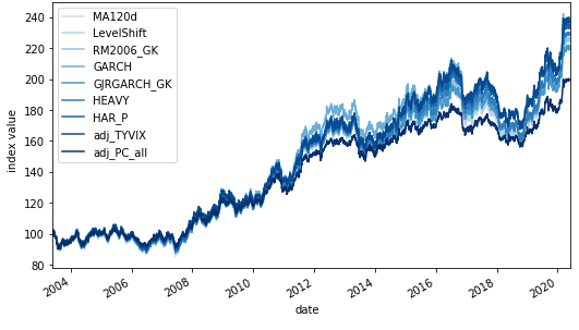
Figure 1. Volatility targeting model price evolution

2.1. Mathematical formulation

We have $n=9$ models. Each model predicts a volatility for the rolled U.S. 10-year note future contract that we shall call ”bond future” in the remainder of this paper. The bond future’s daily returns are denoted by $r^{bond}_{t}$ and typically range from -2 to 2 percents with a daily average value of a few basis points and a daily standard deviation 10 to 50 times higher and ranging from 20 to 70 basis points. By these standards, the bond future’s market is hard to predict and has a lot of noise making its forecast a difficult exercise. Hence, using some volatility forecast to scale position makes a lot of sense. These forecasts are then used to compute the allocation to the bond future’s models. Mathematically, if the target volatility of the strategy is denoted by $\sigma_{target}$ and if the model $i$ predicts a bond future’s volatility $\sigma^{i,pred}_{t-1}$, based on information up to $t-1$, the allocation in the bond future’s model $i$ at time $t$ is given by the ratio between the target volatility and the predicted volatility: $k^{i}_{t-1}=\frac{\sigma_{target}}{\sigma^{i,pred}_{t-1}}$.

Hence, we can compute the daily amounts invested in each of the bond future volatility models and create a corresponding time series of returns $r^{i}_{t}=k^{i}_{t-1}\times r^{bond}_{t}$, consisting of investing in the bond future according to the allocation computed by the volatility targeting model $i$. This provides $n$ time series of compounded returns whose values are given by $P^{i}_{t}=\prod_{u=t_{1}...t}\left(1+r^{i}_{u}\right)$. Our RL problem then boils down to selecting the optimal portfolio allocation (with respect to the cumulative reward) in each model-based RL strategies $a^{i}_{t}$ such that the portfolio weights sum up to one and are non-negative $\sum_{i=1..n}a^{i}_{t}=1$ and $a^{i}_{t}\geq 0$ for any $i=1..n$. These allocations are precisely the continuous actions of the DRL model. This is not an easy problem as the different volatility forecasts are quite similar. Hence, the $n$ time series of compounded returns look almost the same, making this RL problem non-trivial. Our aim is, in a sense, to distinguish between the indistinguishable strategies that are presented in figure 1. More precisely, figure 1 provides the evolution of the net value of an investment strategy that follows the different volatility targeting models.

Compared to standard portfolio allocation problems, these strategies’ returns are highly correlated and similar as presented by the correlation matrix 2, with a lowest correlation of 97%. The correlation is computed as the Pearson correlation over the full data set from 2004 to 2020.

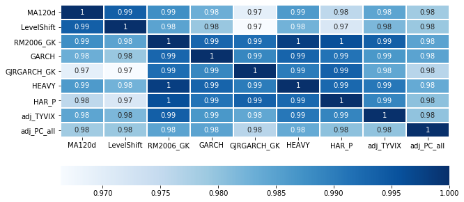
Figure 2. Correlation between the different volatility targeting models’ returns

Following Sutton and Barto (2018), we formulate this RL problem as a Markov Decision Process (MDP) problem. We define our MDP with a 6-tuple $\mathcal{M}=(T,\gamma,\mathcal{S},\mathcal{A},P,r)$ where $T$ is the (possibly infinite) decision horizon, $\gamma\in\left]0,1\right]$ the discount factor, $\mathcal{S}$ the state space, $\mathcal{A}$ the action space, $p(s_{t+1}|s_{t},a_{t})$ the transition probability from the state $s_{t}$ to $s_{t+1}$ given that the agent has chosen the action $a_{t}$, and $r(s_{t},a_{t})$ the reward for a state $s_{t}$ and an action $a_{t}$.

The agent’s objective is to maximize its expected cumulative returns, given the start of the distribution. If we denote by $\pi$ the policy mapping specifying the action to choose in a particular state, $\pi:\mathcal{S}\to\mathcal{A}$, the agent wants to maximize the expected cumulative returns. This is written as: $J^{\pi}=\mathbb{E}_{s_{t}\sim P,a_{t}\sim\pi}\left[\sum_{t=1}^{T}\gamma^{t-1}r(s_{t},a_{t})\right]$.

MDP assumes that we know all the states of the environment and have all the information to make the optimal decision in every state.

From a practical standpoint, there are a few limitations to accommodate. First of all, the Markov property implies that knowing the current state is sufficient. Hence, we modify the RL setting by taking a pseudo state formed with a set of past observations $(o_{t-n},o_{t-n-1},\ldots,o_{t-1},o_{t})$. The trade-off is to take enough past observations to be close to a Markovian status without taking too many observations which would result in noisy states.

In our settings, the actions are continuous and consist in finding at time $t$ the portfolio allocations $a^{i}_{t}$ in each volatility targeting model. We denote by $a_{t}=\left(a^{1}_{t},...,a^{n}_{t}\right)^{T}$ the portfolio weights vector.

Figure 3. Overall architecture

Likewise, we denote by $p_{t}=\left(p^{1}_{t},...,p^{n}_{t}\right)^{T}$ the closing price vector, and by $u_{t}=p_{t}\oslash p_{t-1}=\left(p^{1}_{t}/p^{1}_{t-1},...,p^{n}_{t}/p^{n}_{t-1}\right)^{T}$ the price relative difference vector, where $\oslash$ denotes the element-wise division,

and by $r_{t}=\left(p^{1}_{t}/p^{1}_{t-1}-1,...,p^{n}_{t}/p^{n}_{t-1}-1\right)^{T}$ the returns vector which is also the percentage change of each closing prices $p^{1}_{t},...,p^{n}_{t}$. Due to price change in the market, at the end of the same period, the weights evolve according to $w_{t-1}=(u_{t-1}\odot a_{t-1})/(u_{t-1}.a_{t-1})$ where $\odot$ is the element-wise multiplication, and . the scalar product.

The goal of the agent at time $t$ is hence to reallocate the portfolio vector from $w^{t-1}$ to $a_{t}$ by buying and selling the relevant assets, taking into account the transaction costs that are given by $\alpha\lvert a_{t}-w_{t-1}\rvert_{1}$ where $\alpha$ is the percentage cost for a transaction (which is quite low for future markets and given by 1 basis point) and $\lvert.|_{1}$ is the $L_{1}$ norm operator. Hence at the end of time $t$, the agent receives a portfolio return given by $a_{t}.u_{t}-\alpha\lvert a_{t}-w_{t-1}\rvert_{1}$. The cumulative reward corresponds to the sum of the logarithmic returns of the portfolio strategy given by $\mathbb{E}\left[\prod_{t=1}^{T}\log\left(a_{t}.u_{t}-\alpha\lvert a_{t}-w_{t-1}\rvert_{1}\right)\right]$, which is easier to process in a tensor flow graph as a log sum expression and is naturally given by $\mathbb{E}\left[\log\left(\sum_{t=1}^{T}a_{t}.u_{t}-\alpha|a_{t}-w_{t-1}|_{1}\right)\right]$.

Actions are modeled by a multi-input, multi-layer convolution network whose details are given by Figure 5. It has been shown that convolution networks are better for selecting features in portfolio allocation problem Benhamou et al. (2021b), Benhamou et al. (2021a) and Benhamou et al. (2020b). The goal of the model-free RL method is to find the network parameters. This is done by an adversarial policy gradient method summarized by the algorithm 1 using traditional Adam optimization so that we have the benefit of adaptive gradient descent with root mean square propagation Kingma and Ba (2014) with a learning rate of 1% and a number of iteration steps of 100,000 with an early stop criterion if the cumulative reward does not improve after 15 full episodes. Because each episode is run on the same financial data, we use on purpose a vanilla policy gradient algorithm to take advantage of the stability of the environment rather than to use more advanced DRL agents like TRPO, DDPG or TD3 that would add on top of our model free RL layer some extra complexity and noise.

Algorithm 1 Adversarial Policy Gradient

1:  Input: initial policy parameters $\theta$, empty replay buffer $\mathcal{D}$

2:  repeat

3:     Reset replay buffer

4:     while not Terminal do

5:        Observe observation $o$ and select action $a=\pi_{\theta}(o)$ with probability $p$ and random action with probability $1-p$,

6:        Execute $a$ in the environment

7:        Observe next observation $o^{\prime}$, reward $r$, and done signal $d$ to indicate whether $o^{\prime}$ is terminal

8:        Apply noise to next observation $o^{\prime}$

9:        Store $(o,a,o^{\prime})$ in replay buffer $\mathcal{D}$

10:        if Terminal then

11:           for however many updates in $\mathcal{D}$ do

12:              Compute final reward $R$

13:           end for

14:           Update network parameter with Adam gradient ascent $\@vec{\theta}\longrightarrow\@vec{\theta}+\lambda\nabla_{\@vec{\theta}}J_{[0,t]}(\pi_{\@vec{\theta}})$

15:        end if

16:     end while

17:  until Convergence

2.2. Benchmarks

2.2.1. Markowitz

In order to benchmark our DRL approach, we need to compare to traditional financial methods. Markowitz allocation as presented in Markowitz (1952) is a widely-used benchmark in portfolio allocation as it is a straightforward and intuitive mix between performance and risk. In this approach, risk is represented by the variance of the portfolio. Hence, the Markowitz portfolio minimizes variance for a given expected return, which is solved by standard quadratic programming optimization. If we denote by $\mu=(\mu_{1},...,\mu_{n})^{T}$ the expected returns for our $n$ model strategies and by $\Sigma$ the covariance matrix of these strategies’ returns, and by $r_{min}$ the targeted minimum return, the Markowitz optimization problem reads

Minimize $$w^{T}\Sigma w$$

subject to $$\mu^{T}w\geq r_{min},\sum_{i=1\ldots l}w_{i}=1,w\geq 0$$

2.2.2. Average

Another classical benchmark model for indistinguishable strategies, is the arithmetic average of all the volatility targeting models. This seemingly naive benchmark is indeed performing quite well as it mixes diversification and mean reversion effects.

2.2.3. Follow the winner

Another common strategy is to select the best performer of the past year, and use it the subsequent year. It replicates the standard investor’s behavior that selects strategies that have performed well in the past.

2.3. Procedure and walk forward analysis

The whole procedure is summarized by Figure 3. We have $n$ models that represent the dynamics of the market volatility. We then add the volatility and the contextual information to the states, thereby yielding augmented states. The latter procedure is presented as the second step of the process. We then use a model-free RL approach to find the portfolio allocation among the various volatility targeting models, corresponding to steps 3 and 4. In order to test the robustness of our resulting DRL model, we introduce a new methodology called walk forward analysis.

2.3.1. Walk forward analysis

In machine learning, the standard approach is to do $k$-fold cross-validation. This approach breaks the chronology of data and potentially uses past data in the test set. Rather, we can take sliding test set and take past data as training data. To ensure some stability, we favor to add incrementally new data in the training set, at each new step.

Figure 4. Overall training process

This method is sometimes referred to as ”anchored walk forward” as we have anchored training data. Finally, as the test set is always after the training set, walk forward analysis gives less steps compared with cross-validation. In practice, and for our given data set, we train our models from 2000 to the end of 2013 (giving us at least 14 years of data) and use a repetitive test period of one year from 2014 onward. Once a model has been selected, we also test its statistical significance, defined as the difference between the returns of two time series. We therefore do a T-test to validate how different these time series are. The whole process is summarized by Figure 4.

2.3.2. Model architecture

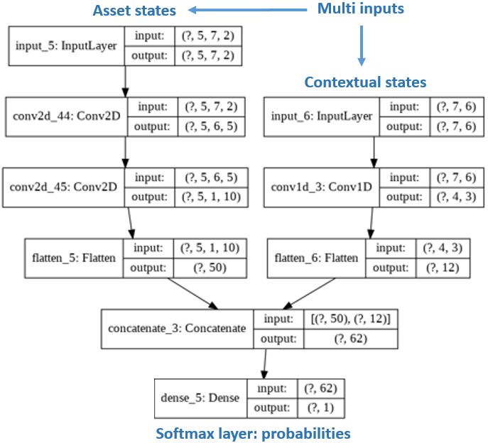
Figure 5. Multi-input DRL network

The states consist in two different types of data: the asset inputs and the contextual inputs.

Asset inputs are a truncated portion of the time series of financial returns of the volatility targeting models and of the volatility of these returns computed over a period of 20 observations. So if we denote by $r^{i}_{t}$ the returns of model $i$ at time $t$, and by $\sigma^{i}_{t}$ the standard deviation of returns over the last $d=20$ periods, asset inputs are given by a 3-D tensor denoted by $A_{t}=\left[R_{t},V_{t}\right]$, with

$R_{t}=\left(\!\begin{array}[]{c}r^{1}_{t-n}\,\,...\,\,r^{1}_{t}\\ ...\,\,...\,\,...\\ r^{m}_{t-n}\,\,....\,\,r^{m}_{t}\end{array}\!\right)\!\ \ \\ \ \text{and }V_{t}=\left(\!\begin{array}[]{c}\sigma^{1}_{t-n}\,\,...\,\,\sigma^{1}_{t}\\ ...\,\,...\,\,...\\ \sigma^{m}_{t-n}\,\,....\,\,\sigma^{m}_{t}\end{array}\!\right)$.

This setting with two layers (past returns and past volatilities) is very different from the one presented in Jiang and Liang (2016); Zhengyao et al. (2017); Liang et al. (2018) that uses layers representing open, high, low and close prices, which are not necessarily available for volatility target models. Adding volatility is crucial to detect regime change and is surprisingly absent from these works.

Contextual inputs are a truncated portion of the time series of additional data that represent contextual information. Contextual information enables our DRL agent to learn the context, and are, in our problem, short-term and long-term risk appetite indices and short-term and long-term macro signals. Additionally, we include the maximum and minimum portfolio strategies return and the maximum portfolio strategies volatility. Similarly to asset inputs, standard deviations is useful to detect regime changes. Contextual observations are stored in a 2D matrix denoted by $C_{t}$ with stacked past $p$ individual contextual observations. The contextual state reads

$C_{t}=\left(\!\!\begin{array}[]{c }c^{1}_{t-n}\,\,...\,\,c^{1}_{t}\\ ...\,\,...\,\,...\\ c^{p}_{t-n}\,\,....\,\,c^{p}_{t}\end{array}\!\!\!\right)$.

The output of the network is a softmax layer that provides the various allocations. As the dimensions of the assets and the contextual inputs are different, the network is a multi-input network with various convolutional layers and a final softmax dense layer as represented in Figure 5.

2.3.3. Features sensitivity analysis

One of the challenges of neural networks relies in the difficulty to provide explainability about their behaviors. Inspired by computer vision, we present a methodology here that enables us to relate features to action. This concept is based on features sensitivity analysis. Simply speaking, our neural network is a multi-variate function. Its inputs include all our features, strategies, historical performances, standard deviations, contextual information, short-term and long-term macro signals and risk appetite indices. We denote these inputs by $X$, which lives in $\mathbb{R}^{k}$ where $k$ is the number of features. Its outputs are the action vector $Y$, which is an $n$-d array with elements between 0 and 1. This action vector lives in an image set denoted by $\mathcal{Y}$, which is a subset of $\mathbb{R}^{n}$ . Hence, the neural network is a function $\Phi:\mathbb{R}^{k}\to\mathcal{Y}$ with $\Phi(X)=Y$. In order to project the various partial derivatives, we take the L1 norm (denoted by $|.|_{1}$) of the different partial derivatives as follows: $|\frac{\partial\Phi(X)}{\partial X}|_{1}$. The choice of the L1 norm is arbitrary but is intuitively motivated by the fact that we want to scale the distance of the gradient linearly.

In order to measure the sensitivity of the outputs, simply speaking, we change the initial feature by its mean value over the last $d$ periods. This is inspired by a ”what if” analysis where we would like to measure the impact of changing the feature from its mean value to its current value. In computer vision, the practice is not to use the mean value but rather to switch off the pixel and set it to the black pixel. In our case, using a zero value would not be relevant as this would favor large features. We are really interested here in measuring the sensitivity of our actions when a feature deviates from its mean value.

The resulting value is computed numerically and provides us for each feature a feature importance. We rank these features importance and assign arbitrarily the value $100$ to the largest and $0$ to the lowest. This provides us with the following features importance plot given below 6. We can notice that the HAR returns and volatility are the most important features, followed by various returns and volatility for the TYVIX model. Although returns and volatility are dominating among the most important features, macro signals 0d observations comes as the 12th most important feature over 70 features with a very high score of 84.2. The features sensitivity analysis confirms two things: i) it is useful to include volatility features as they are good predictors of regime changes, ii) contextual information plays a role as illustrated by the macro signal.

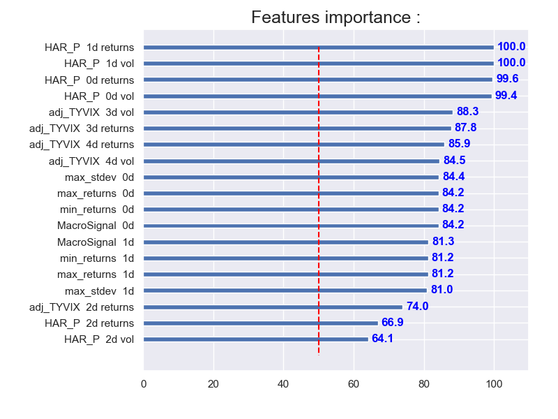
Figure 6. Model explainability

3. Out of sample results

In this section, we compare the various models: the deep RL model (DRL1) using states with contextual inputs and standard deviation, the deep RL model without contextual inputs and standard deviation (DRL2), the average strategy, the Markowitz portfolio and the ”the winner” strategy. The results are the combination of the 7 distinct test periods: each year from 2014 to 2020. The resulting performance is plotted in Figure 7. We notice that the deepRL model with contextual information and standard deviation is substantially higher than the other models in terms of performance as it ends at 157, whereas other models (the deepRL with no context, the average, the Markowitz and ”the winner” model) end at 147.6, 147.8, 145.5, 143.4 respectively.

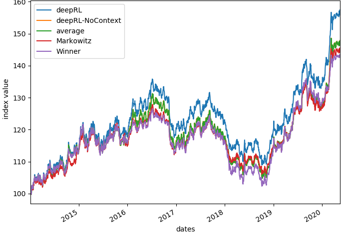
Figure 7. Model comparison

To make such a performance, the DRL model needs to frequently rebalance between the various models (Figure 8) with dominant allocations in GARCH and TYVIX models (Figure 9).

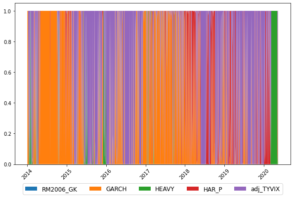
Figure 8. DRL portfolio allocation

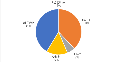
Figure 9. Average model allocation

3.1. Results description

3.1.1. Risk metrics

We provide various statistics in Table 1 for different time horizons: 1, 3 and 5 years. For each horizon, we put the best model, according to the column’s criterion, in bold. The Sharpe and Sortino ratios are computed on daily returns. Maximum drawdown (written as mdd in the table), which is the maximum observed loss from a peak to a trough for a portfolio, is also computed on daily returns. DRL1 is the DRL model with standard deviations and contextual information, while DRL2 is a model with no contextual information and no standard deviation. Overall, DLR1, the DRL model with contextual information and standard deviation, performs better for 1, 3 and 5 years except for three-year maximum drawdown. Globally, it provides a 1% increase in annual net return for a 5-year horizon. It also increases the Sharpe ratio by 0.1 and is able to reduce most of the maximum drawdowns except for the 3-year period. Markowitz portfolio selection and ”the winner” strategy, which are both traditional financial methods heavily used by practitioners, do not work that well compared with a naive arithmetic average and furthermore when compared to the DRL model with context and standard deviation inputs. A potential explanation may come from the fact that these volatility targeting strategies are very similar making the diversification effects non effective.

Table 1. Models comparison over 1, 3, 5 years

	return	sharpe	sortino	mdd	mdd/vol
			1 Year
DRL1	22.659	2.169	2.419	- 6.416	- 0.614
DRL2	20.712	2.014	2.167	- 6.584	- 0.640
Average	20.639	2.012	2.166	- 6.560	- 0.639
Markowitz	19.370	1.941	2.077	- 6.819	- 0.683
Winner	17.838	1.910	2.062	- 6.334	- 0.678
			3 Years
DRL1	8.056	0.835	0.899	- 17.247	- 1.787
DRL2	7.308	0.783	0.834	- 16.912	- 1.812
Average	7.667	0.822	0.876	- 16.882	- 1.810
Markowitz	7.228	0.828	0.891	- 16.961	- 1.869
Winner	6.776	0.712	0.754	- 17.770	- 1.867
			5 Years
DRL1	6.302	0.651	0.684	- 19.794	- 2.044
DRL2	5.220	0.565	0.584	- 20.211	- 2.187
Average	5.339	0.579	0.599	- 20.168	- 2.187
Markowitz	4.947	0.569	0.587	- 19.837	- 2.074
Winner	4.633	0.508	0.526	- 19.818	- 2.095

3.1.2. Statistical significance

Following our methodology described in 4, once we have computed the results for the various walk-forward test periods, we do a T-statistic test to validate the significance of the result. Given two models, we test the null hypothesis that the difference of the returns running average (computed as $(\sum_{u=0}^{t}r_{u}/t)$ for various times $t$) between the two models is equal to 0. We provide the T-statistic and, in parenthesis, the p-value. We take a p-value threshold of 5%, and put the cases where we can reject the null hypothesis in bold in table 2. Hence, we conclude that the DRL model with context (DRL1) model is statistically different from all other models. These results on the running average are quite intuitive as we are able to distinguish the DRL1 model curve from all other curves in Figure 7. Interestingly, we can see that the DRL model without context (DRL2) is not statically different from a pure averaging of the average model that consists in averaging allocation computed by model-based RL approaches.

Table 2. T-statistics and P-values (in parenthesis) for running average returns difference

Avg Return	DRL2	Average	Markowitz	Winner
DRL1	72.1 (0%)	14 (0%)	44.1 (0%)	79.8 (0%)
DRL2		1.2 (22.3%)	24.6 (0%)	10 (0%)
Average			7.6(0%)	0.9 (38.7%)
Markowitz				-13.1 (0%)

3.1.3. Results discussion

It is interesting to understand how the DRL model achieves such a performance as it provides an amazing additional 1% annual return over 5 years, and an increase in Sharpe ratio of 0.10. This is done simply by selecting the right strategies at the right time. This helps us to confirm that the adaptive learning thanks to the model free RL is somehow able to pick up regime changes. We notice that the DRL model selects the GARCH model quite often and, more recently, the HAR and HEAVY model (Figure 8). When targeting a given volatility level, capital weights are inversely proportional to the volatility estimates. Hence, lower volatility estimates give higher weights and in a bullish market give higher returns. Conversely, higher volatility estimates drive capital weights lower and have better performance in a bearish market. The allocation of these models evolve quite a bit as shown by Figure 10, which plots the rank of the first 5 models.

Figure 10. Volatility estimates rank

We can therefore test if the DRL model has a tendency to select volatility targeting models that favor lower volatility estimates. If we plot the occurrence of rank by dominant model for the DRL model, we observe that the DRL model selects the lowest volatility estimate model quite often (38.2% of the time) but also tends to select the highest volatility models giving a U shape to the occurrence of rank as shown in figure 11. This U shape confirms two things: i) the model has a tendency to select either the lowest or highest volatility estimates models, which are known to perform best in bullish markets or bearish markets (however, it does not select these models blindly as it is able to time when to select the lowest or highest volatility estimates); ii) the DRL model is able to reduce maximum drawdowns while increasing net annual returns as seen in Table 1. This capacity to simultaneously increase net annual returns and decrease maximum drawdowns indicates a capacity to detect regime changes. Indeed, a random guess would only increase the leverage when selecting lowest volatility estimates, thus resulting in higher maximum drawdowns.

Figure 11. Occurrence of rank for the DRL model

3.2. Benefits of DRL

The advantages of context based DRL are numerous: (i) by design, DRL directly maps market conditions to actions and can thus adapt to regime changes, (ii) DRL can incorporate additional data and be a multi-input method, as opposed to more traditional optimization methods.

3.3. Future work

As nice as this may look, there is room for improvement as more contextual data and architectural networks choices could be tested as well as other DRL agents like DDPG, TRPO or TD3. It is also worth mentioning that the analysis has been conducted on a single financial instrument and a relatively short out-of-sample period. Expanding this analysis further in the past would cover more various regimes (recessions, inflationary, growth, etc.) and potentially improve the statistical relevance of this study at the cost of losing relevance for more recent data. Another lead consists of applying the same methodology to a much wider ensemble of securities and identify specific statistical features based on distinct geographic and asset sectors.

4. Conclusion

In this work, we propose to create an adaptive learning method that combines model-based and model-free RL approaches to address volatility regime changes in financial markets. The model-based approach enables to capture efficiently the volatility dynamics while the model-free RL approach to time when to switch from one to another model. This combination enables us to have an adaptive agent that switches between different dynamics. We strengthen the model-free RL step with additional inputs like volatility and macro and risk appetite signals that act as contextual information. The ability of this method to reduce risk and profitability are verified when compared to the various financial benchmarks. The use of successive training and testing sets enables us to stress test the robustness of the resulting agent. Features sensitivity analysis confirms the importance of volatility and contextual variables and explains in part the DRL agent’s better performance. Last but not least, statistical tests validate that results are statistically significant from a pure averaging method of all model-based RL allocations.

References

- (1)
- Benhamou (2018) Eric Benhamou. 2018. Trend without hiccups: a Kalman filter approach. ssrn.1808.03297 (2018).
- Benhamou (2019) Eric Benhamou. 2019. Connecting Sharpe ratio and Student t-statistic, and beyond. ArXiv (2019). arXiv:1808.04233 [q-fin.ST]
- Benhamou and Guez (2018) Eric Benhamou and Beatrice Guez. 2018. Incremental Sharpe and other performance ratios. Journal of Statistical and Econometric Methods 2018 (2018).
- Benhamou et al. (2019a) Eric Benhamou, Beatrice Guez, and Nicolas Paris1. 2019a. Omega and Sharpe ratio. ArXiv (2019). arXiv:1911.10254 [q-fin.RM]
- Benhamou et al. (2019b) Eric Benhamou, David Saltiel, Beatrice Guez, and Nicolas Paris. 2019b. Testing Sharpe ratio: luck or skill? ArXiv (2019). arXiv:1905.08042 [q-fin.RM]
- Benhamou et al. (2021a) Eric Benhamou, David Saltiel, Jean-Jacques Ohana, and Jamal Atif. 2021a. Detecting and adapting to crisis pattern with context based Deep Reinforcement Learning. In International Conference on Pattern Recognition (ICPR). IEEE Computer Society.
- Benhamou et al. (2021b) Eric Benhamou, David Saltiel, Jean Jacques Ohana, Jamal Atif, and Rida Laraki. 2021b. Deep Reinforcement Learning (DRL) for Portfolio Allocation. In Machine Learning and Knowledge Discovery in Databases. Applied Data Science and Demo Track, Yuxiao Dong, Georgiana Ifrim, Dunja Mladenić, Craig Saunders, and Sofie Van Hoecke (Eds.). Springer International Publishing, Cham, 527–531.
- Benhamou et al. (2021c) Eric Benhamou, David Saltiel, Sandrine Ungari, and Rida Laraki Abhishek Mukhopadhyay, Jamal Atif. 2021c. Knowledge discovery with Deep RL for selecting financial hedges. In AAAI: KDF. AAAI Press.
- Benhamou et al. (2020a) Eric Benhamou, David Saltiel, Sandrine Ungari, and Abhishek Mukhopadhyay. 2020a. Bridging the gap between Markowitz planning and deep reinforcement learning. In Proceedings of the 30th International Conference on Automated Planning and Scheduling (ICAPS): PRL. AAAI Press.
- Benhamou et al. (2020b) Eric Benhamou, David Saltiel, Sandrine Ungari, and Abhishek Mukhopadhyay. 2020b. Time your hedge with Deep Reinforcement Learning. In Proceedings of the 30th International Conference on Automated Planning and Scheduling (ICAPS): FinPlan. AAAI Press.
- Chebotar et al. (2017) Yevgen Chebotar, Karol Hausman, Marvin Zhang, Gaurav Sukhatme, Stefan Schaal, and Sergey Levine. 2017. Combining Model-Based and Model-Free Updates for Trajectory-Centric Reinforcement Learning. In PMLR (Proceedings of Machine Learning Research), Doina Precup and Yee Whye Teh (Eds.), Vol. 70. PMLR, International Convention Centre, Sydney, Australia, 703–711.
- Clavera et al. (2018) Ignasi Clavera, Jonas Rothfuss, John Schulman, Yasuhiro Fujita, Tamim Asfour, and Pieter Abbeel. 2018. Model-Based Reinforcement Learning via Meta-Policy Optimization. arXiv:1809.05214 http://arxiv.org/abs/1809.05214
- Deisenroth et al. (2014) M. Deisenroth, D. Fox, and C. Rasmussen. 2014. Gaussian processes for data-efficient learning in robotics and control.
- Deisenroth and Rasmussen (2011) Marc Deisenroth and Carl E Rasmussen. 2011. PILCO: A model-based and data-efficient approach to policy search.
- Deisenroth et al. (2011) Marc Peter Deisenroth, Carl Edward Rasmussen, and Dieter Fox. 2011. Learning to Control a Low-Cost Manipulator using Data-Efficient Reinforcement Learning.
- Depeweg et al. (2016) Stefan Depeweg, José Miguel Hernández-Lobato, Finale Doshi-Velez, and Steffen Udluft. 2016. Learning and policy search in stochastic dynamical systems with bayesian neural networks.
- Dias et al. (2015) José Dias, Jeroen Vermunt, and Sofia Ramos. 2015. Clustering financial time series: New insights from an extended hidden Markov model. European Journal of Operational Research 243 (06 2015), 852–864.
- Dreyer and Hubrich (2017) Anna Dreyer and Stefan Hubrich. 2017. Tail Risk Mitigation with Managed Volatility Strategies.
- Ebert et al. (2018) Frederik Ebert, Chelsea Finn, Sudeep Dasari, Annie Xie, Alex X. Lee, and Sergey Levine. 2018. Visual Foresight: Model-Based Deep Reinforcement Learning for Vision-Based Robotic Control.
- Feinberg et al. (2018) Vladimir Feinberg, Alvin Wan, Ion Stoica, Michael I. Jordan, Joseph E. Gonzalez, and Sergey Levine. 2018. Model-Based Value Estimation for Efficient Model-Free Reinforcement Learning. arXiv:1803.00101 http://arxiv.org/abs/1803.00101
- Freitas et al. (2009) Fabio Freitas, Alberto De Souza, and Ailson Almeida. 2009. Prediction-based portfolio optimization model using neural networks. Neurocomputing 72 (06 2009), 2155–2170.
- Gal et al. (2016) Yain Gal, Rowan McAllister, and Carl E. Rasmussen. 2016. Improving PILCO with Bayesian Neural Network Dynamics Models.
- Glosten et al. (1993) Lawrence R Glosten, Ravi Jagannathan, and David E Runkle. 1993. On the Relation between the Expected Value and the Volatility of the Nominal Excess Return on Stocks. Journal of Finance 48, 5 (1993), 1779–1801.
- Haarnoja et al. (2018) Tuomas Haarnoja, Aurick Zhou, Pieter Abbeel, and Sergey Levine. 2018. Soft Actor-Critic: Off-Policy Maximum Entropy Deep Reinforcement Learning with a Stochastic Actor.
- Heaton et al. (2017) J. B. Heaton, N. G. Polson, and J. H. Witte. 2017. Deep learning for finance: deep portfolios. Applied Stochastic Models in Business and Industry 33, 1 (2017), 3–12.
- Hocquard et al. (2013) Alexandre Hocquard, S. Ng, and N. Papageorgiou. 2013. A Constant-Volatility Framework for Managing Tail Risk. The Journal of Portfolio Management 39 (2013), 28–40.
- Janner et al. (2019) Michael Janner, Justin Fu, Marvin Zhang, and Sergey Levine. 2019. When to Trust Your Model: Model-Based Policy Optimization. arXiv:1906.08253 http://arxiv.org/abs/1906.08253
- Jiang and Liang (2016) Zhengyao Jiang and Jinjun Liang. 2016. Cryptocurrency Portfolio Management with Deep Reinforcement Learning. arXiv:1612.01277
- Kaelbling et al. (1996) Leslie Pack Kaelbling, Michael L. Littman, and Andrew P. Moore. 1996. Reinforcement Learning: A Survey. Journal of Artificial Intelligence Research 4 (1996), 237–285.
- Kaiser et al. (2019) Lukasz Kaiser, Mohammad Babaeizadeh, Piotr Milos, Blazej Osinski, Roy H. Campbell, Konrad Czechowski, Dumitru Erhan, Chelsea Finn, Piotr Kozakowsi, Sergey Levine, Ryan Sepassi, George Tucker, and Henryk Michalewski. 2019. Model-Based Reinforcement Learning for Atari.
- Kingma and Ba (2014) Diederik Kingma and Jimmy Ba. 2014. Adam: A Method for Stochastic Optimization.
- Kumar et al. (2016) Vikash Kumar, Emanuel Todorov, and Sergey Levine. 2016. Optimal control with learned local models: Application to dexterous manipulation. , 378–383 pages.
- Levine and Koltun (2013) Sergey Levine and Vladlen Koltun. 2013. Guided Policy Search. , 9 pages. http://proceedings.mlr.press/v28/levine13.html
- Li et al. (2019) Xinyi Li, Yinchuan Li, Yuancheng Zhan, and Xiao-Yang Liu. 2019. Optimistic Bull or Pessimistic Bear: Adaptive Deep Reinforcement Learning for Stock Portfolio Allocation.
- Liang et al. (2018) Liang et al. 2018. Adversarial Deep Reinforcement Learning in Portfolio Management. arXiv:1808.09940 [q-fin.PM]
- Lillicrap et al. (2016) Timothy P. Lillicrap, Jonathan J. Hunt, Alexander Pritzel, Nicolas Heess, Tom Erez, Yuval Tassa, David Silver, and Daan Wierstra. 2016. Continuous control with deep reinforcement learning.
- Liu et al. (2020) Yang Liu, Qi Liu, Hongke Zhao, Zhen Pan, and Chuanren Liu. 2020. Adaptive Quantitative Trading: an Imitative Deep Reinforcement Learning Approach.
- Markowitz (1952) Harry Markowitz. 1952. Portfolio Selection. The Journal of Finance 7, 1 (March 1952), 77–91.
- Mnih et al. (2015) Volodymyr Mnih, Koray Kavukcuoglu, David Silver, Andrei Rusu, Joel Veness, Marc Bellemare, Alex Graves, Martin Riedmiller, Andreas Fidjeland, Georg Ostrovski, Stig Petersen, Charles Beattie, Amir Sadik, Ioannis Antonoglou, Helen King, Dharshan Kumaran, Daan Wierstra, Shane Legg, and Demis Hassabis. 2015. Human-level control through deep reinforcement learning. Nature 518 (02 2015), 529–33.
- Moerland et al. (2020) Thomas M. Moerland, Joost Broekens, and Catholijn M. Jonker. 2020. Model-based Reinforcement Learning: A Survey. arXiv:2006.16712 [cs.LG]
- Nagabandi et al. (2018) Anusha Nagabandi, Gregory Kahn, Ronald Fearing, and Sergey Levine. 2018. Neural Network Dynamics for Model-Based Deep Reinforcement Learning with Model-Free Fine-Tuning. , 7559–7566 pages. https://doi.org/10.1109/ICRA.2018.8463189
- Niaki and Hoseinzade (2013) Seyed Niaki and Saeid Hoseinzade. 2013. Forecasting S&P 500 index using artificial neural networks and design of experiments. Journal of Industrial Engineering International 9 (02 2013).
- Noureldin and Shephard (2012) Diaa Noureldin and Neil Shephard. 2012. Multivariate high-frequency-based volatility (HEAVY) models. , 907–933 pages.
- Oh et al. (2015) Junhyuk Oh, Xiaoxiao Guo, Honglak Lee, Richard Lewis, and Satinder Singh. 2015. Action-Conditional Video Prediction using Deep Networks in Atari Games.
- Perchet et al. (2016) Romain Perchet, Raul Leote de Carvalho, Thomas Heckel, and Pierre Moulin. 2016. Predicting the Success of Volatility Targeting Strategies: Application to Equities and Other Asset Classes. , 21–38 pages.
- Pong et al. (2018) Vitchyr Pong, Shixiang Gu, Murtaza Dalal, and Sergey Levine. 2018. Temporal Difference Models: Model-Free Deep RL for Model-Based Control. arXiv:1802.09081 http://arxiv.org/abs/1802.09081
- Salhi et al. (2015) Khaled Salhi, Madalina Deaconu, Antoine Lejay, Nicolas Champagnat, and Nicolas Navet. 2015. Regime switching model for financial data: empirical risk analysis.
- Sutton and Barto (2018) Richard S. Sutton and Andrew G. Barto. 2018. Reinforcement Learning: An Introduction. The MIT Press, The MIT Press.
- van Hasselt et al. (2019) Hado van Hasselt, Matteo Hessel, and John Aslanides. 2019. When to use parametric models in reinforcement learning? arXiv:1906.05243 http://arxiv.org/abs/1906.05243
- Wang and Zhou (2019) Haoran Wang and Xun Yu Zhou. 2019. Continuous-Time Mean-Variance Portfolio Selection: A Reinforcement Learning Framework. arXiv:1904.11392 [q-fin.PM]
- Xiong et al. (2019) Zhuoran Xiong, Xiao-Yang Liu, Shan Zhong, Hongyang Yang, and Anwar Walid. 2019. Practical Deep Reinforcement Learning Approach for Stock Trading.
- Ye et al. (2020) Yunan Ye, Hengzhi Pei, Boxin Wang, Pin-Yu Chen, Yada Zhu, Ju Xiao, and Bo Li. 2020. Reinforcement-Learning Based Portfolio Management with Augmented Asset Movement Prediction States. In AAAI. AAAI, New York, 1112–1119. https://aaai.org/ojs/index.php/AAAI/article/view/5462
- Yu et al. (2019) Pengqian Yu, Joon Sern Lee, Ilya Kulyatin, Zekun Shi, and Sakyasingha Dasgupta. 2019. Model-based Deep Reinforcement Learning for Financial Portfolio Optimization.
- Zheng et al. (2019) Kai Zheng, Yuying Li, and Weidong Xu. 2019. Regime switching model estimation: spectral clustering hidden Markov model.
- Zhengyao et al. (2017) Zhengyao et al. 2017. Reinforcement Learning Framework for the Financial Portfolio Management Problem. arXiv:1706.10059v2