Fermiology of two-dimensional titanium carbide and nitride MXenes

Abstract

MXenes are a family two-dimensional transition metal carbide and nitride materials, which often exhibit very good metallic conductivity and are thus of great interest for applications in, e.g., flexible electronics, electrocatalysis, and electromagnetic interference shielding. However, surprisingly little is known about the fermiology of MXenes, i.e, the shape and size of their Fermi-surfaces, and its effect on the material properties. One reason for this may be that MXene surfaces are almost always covered by a mixture of functional groups, and studying Fermi-surfaces of disordered systems is cumbersome. Here, we study fermiology of four common Ti-based MXenes as a function of the surface functional group composition. We first calculate the effective band structures of systems with explicit mixed surfaces and observe gradual evolution in the filling of the Ti-d band and resulting shift of Fermi-level. We then demonstrate that these band structures can be closely approximated by using pseudohydrogenated surfaces, and also compare favorably to the experimental angle-resolved photoemission spectroscopy results. By modifying the pseudohydrogen charge we then proceed to plot Fermi-surfaces for all systems and extract their properties, such as the Fermi-surface area and average Fermi-velocity. These are in turn used to evaluate the electrical conductivity with the relaxation time fitted to experimentally measured conductivities.

I Introduction

MXenes are a large class of two-dimensional (2D) materials of transition metal (M) carbides and nitrides (X) Naguib et al. (2012); Gogotsi and Anasori (2019). Distinct from other 2D materials, MXenes are synthesized by etching out layers of atoms from a layered bulk precursor phase. As a result of the etching process, the dangling bonds on the surface are passivated by a mixture of organic groups from the etching solution, such as -O, -OH, and -F Naguib et al. (2011). MXenes are metallic and exhibit very high conductivity in addition to good mechanical properties and easy solution processing. As a result, they have shown great promise for applications in conductive inks, battery electrodes, electromagnetic interference shielding, and various types of sensors Shahzad et al. (2016); Anasori et al. (2017); Fu et al. (2019); Lee and Kim (2020).

Given the large interest on these materials, surprisingly little effort has been devoted to understanding the fundamental properties of their Fermi-surfaces, i.e., fermiology, and its effect on the material properties Matsuda and Hasegawa (2007). Experimentally, Fermi-surfaces are commonly investigated using angle-resolved photoemission spectroscopy (ARPES) Matsuda and Hasegawa (2007); Lasek et al. (2021). ARPES results for delaminated Ti₃C₂, the prototypical MXene, were reported by Schultz et al. Schultz et al. (2019), but since the measured film consists of randomly oriented flakes, the ARPES data was azimuthally averaged, which prevented the extraction of the Fermi-surface shape. Quasiparticle interference within scanning tunneling microscope (STM-QPI) is also often used to gain insight on the Fermi-surface, but requires high quality surface with small density of scattering centers Chen et al. (2017) — a luxury not afforded in the case of MXenes, where the surfaces are covered by a random mixture of organic groups and other residues from the synthesis. In fact, to the best of our knowledge, clean STM images of MXene surfaces have not been reported in the literature. Finally, Fermi-surfaces could be probed via de Haas van Alphen effect Ouisse and Barsoum (2017), but again no reports exist for MXenes.

Also computational studies of Fermi-surfaces are very rare, even when the band structures have been reported in numerous papers and are relatively well understood Xie and Kent (2013); Khazaei et al. (2013, 2017). Hu et al. calculated the Fermi-surface of monolayer and bulk Ti₂C₂(OH)₂ for two different layer stackings Hu et al. (2015). In addition, some insight can be gained from the Fermi-surfaces of the precursor MAX phases, which were presented in Ref. Ouisse and Barsoum, 2017. While the Fermi-surfaces for pure O or OH terminated structures are straightforward to evaluate, since the surfaces are passivated by a mixture of groups (stabilized by strong nearest neighbor interactions between the groups Ibragimova et al. (2019, 2021)) and the electronic structure of O and OH-terminated surfaces differ markedly, it is not clear how the Fermi-surface evolves with changing functional group composition. Calculations for the mixed group surfaces are cumbersome due to requiring the use of supercells and the resulting band folding. The band structures can be unfolded with the effective band structure method, where each state from the supercell Brillouin zone is projected to each of the folded planewaves from the primitive cell Brillouin zone Ku et al. (2010); Popescu and Zunger (2010), but smearing of the bands still complicates the analysis.

In this paper, we show how to overcome these problems and report results for the Fermi-surfaces of Ti₃C₂, Ti₂C, Ti₄N₃, and Ti₂N monolayers with varying O/OH composition. We calculate the effective band structures for mixed group surfaces and show that they can be well approximated by pseudohydrogenated surfaces. We analyze the Fermi-surface properties as a function of the surface group composition and compare the evaluated electrical conductivities to the experiments. We also compare the Ti₃C₂ band structure to those obtained from recent ARPES experiments.

II Methods

All density-functional theory calculations are carried out using VASP software Kresse and Furthmüller (1996a, b), together with projector augmented plane wave method Blöchl (1994). We adopt the Perdew-Burke-Ernzerhof exchange-correlation functional for solids (PBEsol)Perdew et al. (2008). The plane wave cutoff is 550 eV and the Brillouin zone of the primitive cell is sampled with a 16$\times$16 k-point mesh.

The effective band structures (EBS) are calculated using BandUP software Medeiros et al. (2014). The atomic structures for the mixed surfaces were determined via combination of cluster expansion and Monte Carlo simulations in our previous publication Ibragimova et al. (2021), and we use the same 4$\times$4 supercell special quasi-ordered structures as constructed therein.

Electronic band structures are interpolated using BoltzTrap2 software, which is also used for the integration of the transport properties Madsen et al. (2018). We use k-point mesh interpolation factor 200 and temperature 300 K. Fermi-surfaces are analyzed and plotted using the ifermi software Ganose et al. (2021), with interpolation factor 20.

III Results

III.1 Band structures of mixed surface MXenes

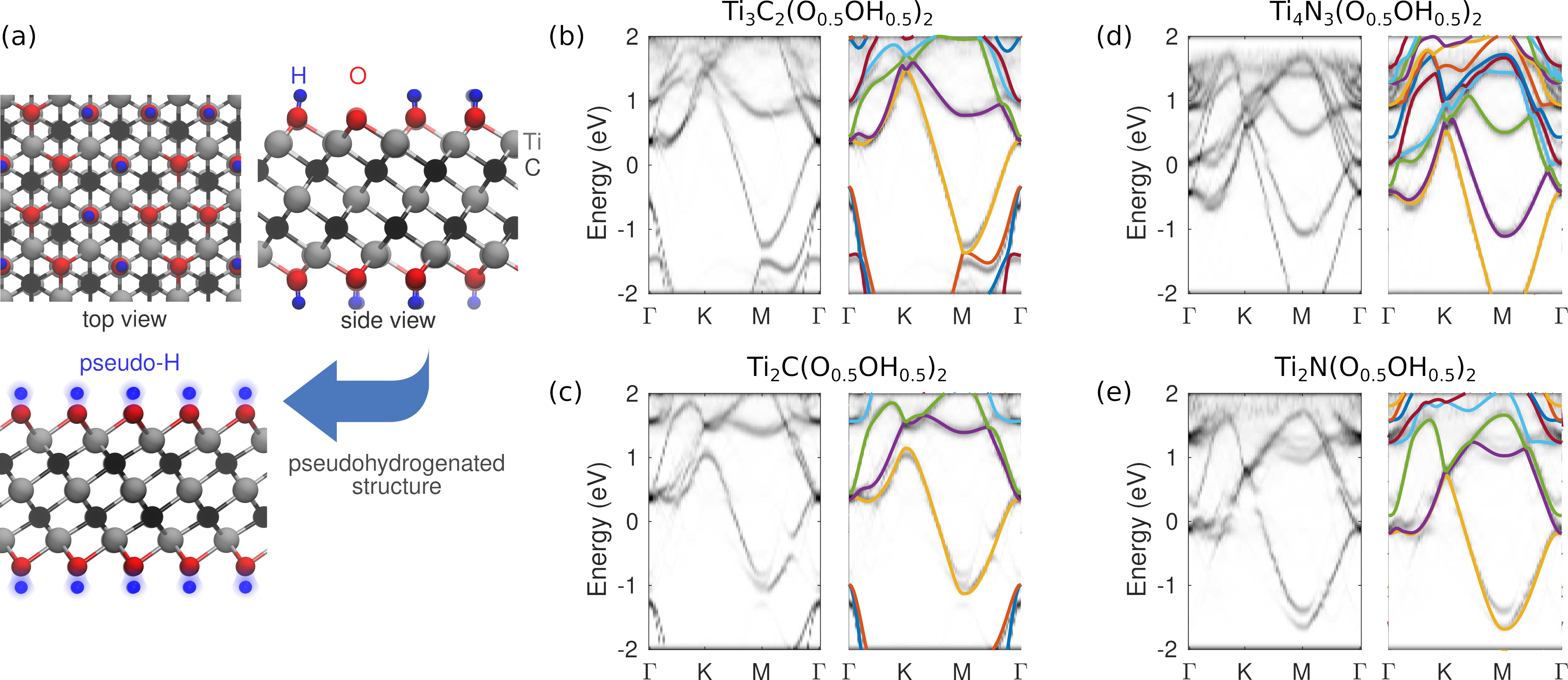
Figure 1: (a) Atomic structure for Ti₃C₂ with a surface functionalized by a mixture of O and OH groups (top) and the corresponding pseudohydrogenated structure (bottom). (b-e) Effective band structures for all materials (left panel) and band structures of pseudohydrogenated surfaces overlaid on the EBS (right panel). Fermi-level is set to zero.

More realistic structural models for the distribution of functional groups were developed by us in Refs. Ibragimova et al., 2019, 2021. As an example, the structure of Ti₃C₂ with O_0.5OH_0.5 surface composition is shown in Fig. 1(a). In the left panels of Fig. 1(b-e) we show the effective band structures for the four Ti-based MXenes with O_0.5OH_0.5 surface composition. From these results, and from comparison to the band structure of pure surfaces (see Figs. 2–3 below), it is clear that the band structures undergo a gradual evolution and there are no extraneous bands arising from the surface groups. The band(s) at the Fermi-level arise from the non-bonding t_2g states of Ti-d character Hu et al. (2017). Consequently, to a very good approximation, the surface groups only control the electron concentration and consequently the Fermi-level position in the metal d-bands, as has been previously assumed Khazaei et al. (2013, 2017). This also suggests that other charge acceptor or donor species could be used just as well for controlling the Fermi-level position.

Given that effective band structures are unwieldy for detailed studies of these materials’ fermiology, we propose to use pseudohydrogenated surfaces to control the Fermi-level position. In practice, we use the primitive cell of a fully OH-terminated structures, but with the H atom replaced by a pseudohydrogen atom with atomic number $Z=0.25$, $0.50$, or $0.75$ (i.e., proton charge is $Ze$ and total electron charge $-Ze$). The pseudohydrogen band structures for $Z=0.5$ are shown on the right panels of Fig. 1(b-e), overlaid on top of the effective band structures. In all cases, the band structures of pseudohydrogenated MXenes agree extremely well with the EBS, thereby further corroborating the physical picture described above.

It is worth noting that we also calculated the band structures for systems with one side fully terminated by O and the other by OH, but the resulting band structures did not agree favorably with the EBS due to broken symmetry. Moreover, such approach would obviously be limited to a O_0.5OH_0.5 composition.

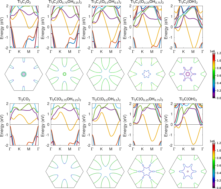
Figure 2: Evolution of the band structures of Ti₃C₂ and Ti₂C with surface group composition. The Fermi-surfaces are plotted under each panel, with the color denoting Fermi-velocity.

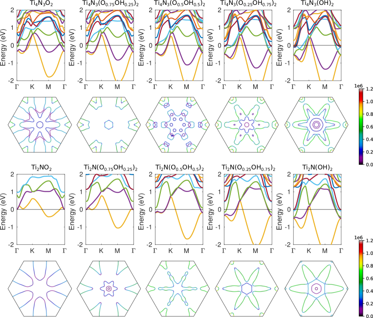
Figure 3: Evolution of the band structures of Ti₄N₃ and Ti₂N with surface group composition. The Fermi-surfaces are plotted under each panel, with the color denoting Fermi-velocity.

The band structure evolution with O/OH composition, for all materials and five different O/OH compositions, are collected in Fig. 2 and 3. From these plots, the gradual change in the band energies is easily resolved.

Based on the analysis by Hu et al. Hu et al. (2017), the states below Fermi-level (red colored band and below in Figs. 2 and 3) arise from bonding state between Ti-d and C-p/N-p ($e_{\rm g}$), and similar to bulk carbides and nitrides Häglund et al. (1993). The states at and above Fermi-level (orange colored band and above) arise from non-bonding $t_{\rm 2g}$ states of Ti-d. In most cases there is a gap between these two band manifolds, but the Fermi-level resides in the Ti-d manifold in all cases except for the fully O-terminated Ti₂C. Due to the larger electronegativity of N, as compared to C, the Ti-N bonding states are clearly lower in energy and lead to a larger gap below the nonbonding states. The Ti-C bands cross the Fermi-level around $\Gamma$-point only for O-rich Ti₃C₂, but thereby prevent it from becoming semiconductor as happens with Ti₂CO₂.

Due to the additional electron(s) in N, as compared to C, there is one additional electron per X atom to fill the M-d bands and consequently Fermi-level resides higher within this band. For instance, the lowest energy band (orange) is exactly half-filled by the one additional electron in the case of Ti${}_{2}N$, whereas the band is empty in the case of Ti₂C. Similar half-filling of the band can be obtained in the case of O_0.5OH_0.5 surface composition of Ti₃C₂ or Ti₂C.

The band fillings can also be readily obtained via electron counting. In the case of Ti₃C₂O₂ and Ti₂CO₂, Ti, C, and O are in the oxidation states +4, -4, and -2, respectively, as in TiC and TiO₂. Upon addition of H atoms (oxidation state +1) and the subsequent occupation of the non-bonding Ti-d band, the charge balance is achieved by decreasing the oxidation state of Ti. The nitrogen atoms (oxidation state -3) have a similar effect.

O/OH composition controls the occupation of the t_2g band, but since it is nonbonding, it should have relatively minor effect on the energetics. Among the purely terminated surfaces, O-terminated surfaces have been predicted to be the most stable, but the mixed surfaces arise in practice due to the strong attractive interactions between the opposite type surface groups Ibragimova et al. (2019, 2021). Consequently, since the surface composition is dominated by the interactions between surface groups, it is rather independent on the M and X species, as we observed in Ref. Ibragimova et al., 2021 (we also note, that the energy gain upon mixing is not captured in the pseudohydrogen models). Even if the O/OH mixing cannot be easily avoided, we expect that the Fermi-level position can still be tuned by introducing alloying in the M and X sublattices.

III.2 Fermi-surface properties

The Fermi-surfaces are plotted below the band structures in Figs. 2 and 3, and colored by the Fermi-velocity. When Fermi-level crosses the lowest energy Ti-d band, it leads to hexagonally symmetric ellipsoids around the M-points. These have fairly large Fermi-velocities, reaching values above $0.5\cdot 10^{6}$ m/s, which is only about factor of two lower than in the highly conducting elemental metals. At large OH concentrations (or any concentration in the case of Ti₄N₃) when the Fermi-level rises to cross the set of states around $\Gamma$-point, the Fermi-surfaces develop more complex features.

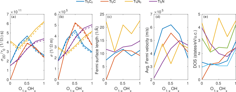
Figure 4: Fermi-surface properties: (a) sheet conductivity, (b) conductivity, (c) Fermi-surface length, (d) Fermi-velocity, and (e) density of states.

With access to Fermi-surfaces of (effectively) mixed surface MXenes, we can next estimate their properties. Since MXenes are known to exhibit excellent electrical conductivity, we evaluated the sheet conductivity within the constant relaxation time approximation (in x-direction) as

$$\sigma_{\rm 2D} =\frac{e^{2}}{2\pi^{2}\hbar}\tau_{0}\int_{E=E_{F}}\frac{v_{x}^{2}(k)}{|v(k)|}dk_{F}$$ (1a)

$$=\frac{e^{2}}{2\pi^{2}\hbar}\tau_{0}\frac{\langle v_{F}\rangle}{2}\cdot l_{F}$$ (1b)

see Supplemental Material for more detailed description.

The sheet conductivities are shown in Fig. 4(a). The solid lines show the results from the full integral (Eq. 1a) and the dashed lines from average Fermi-velocity approximation (Eq. 1b). All four considered MXenes show similar $\sigma_{\rm 2D}/\tau_{0}$, mostly falling within 2–4 $1/\Omega\square$s. The approximation (Eq. 1b) works very well and thus by inspecting the $\langle v_{F}\rangle$ and $l_{F}$ shown in Fig. 4(c,d), we can study their roles in governing the conductivity. Fermi-surface lengths and average Fermi-velocity are similar in Ti₃C₂, Ti₂C, and Ti₂N. Ti₄N₃ shows larger total length due to large number of states crossing the Fermi-level, but the average Fermi-velocities in these states are low. Overall, our results indicate that by simply tuning the surface composition the sheet conductivity cannot be changed by more than about a factor of two.

Trends in electrical conductivity are often evaluated from the density of states (DOS) at Fermi-level, since $l_{F}\sim D_{\rm 2D}(E_{F})\langle v_{F}\rangle$ (cf. Supplemental Material). The DOS at Fermi-level are presented in 4(e) and shows that the trends in the conductivity changes with composition or between different materials cannot be extracted solely from the DOS due to missing the effect of $\langle v_{F}\rangle$.

Experimentally measuring the sheet conductivity of MXene monolayers is challenging, but the conductivity of MXene films has been reported in several publications. In the case of Ti₃C₂ films, conductivities above $10^{5}$ S/m have been reported often Halim et al. (2014); Ling et al. (2014); Shahzad et al. (2016); Liu et al. (2020). Recently a value as high as $1.1\cdot 10^{6}$ S/m was achieved for a high crystalline quality Ti₃C₂ monolayer Lipatov et al. (2021). For other considered materials, the reports are more scarce, but nevertheless fairly similar values can be found: $5\cdot 10^{5}$ S/m for Ti₂N Soundiraraju and George (2017), and $2.3\cdot 10^{5}$ S/m for Ti₂C Halim et al. (2019). It is worth noting, that the conductivity may be governed by interflake contacts and thus also sensitive to the presence of any intercalated species Hart et al. (2019).

In order to estimate the film conductivity, we calculate $\sigma=(\sigma_{\rm 2D}/\tau_{0})\cdot\tau_{0}/t$, where $\tau_{0}$ is the relaxation time and $t$ is the interlayer separation taken from experiments: 10.3, 7.5,Naguib et al. (2012) 14,Urbankowski et al. (2016) and 8.7 ÅSoundiraraju and George (2017) for Ti₃C₂, Ti₂C, Ti₄N₃, and Ti₂N, respectively. Note, that the interlayer separation depends on the preparation method, as, e.g., intercalation of Li can increase the spacing by a few Å. Here we do not attempt to evaluate $\tau_{0}$ from first-principles calculations, but instead from the comparison to experimentally measured conductivities. In Fig. 4(b) we show the results for $\tau_{0}=1$ fs, which yields $\sigma$ values comparable to majority of the experimental reports. The result of Ref. Lipatov et al., 2021 can be reproduced by taking slightly larger $\tau\approx 2-3$ fs, depending on the surface composition. The lower $\tau_{0}$ in earlier reports may then be ascribed to larger number of defects caused by the strong etching, although the interflake contacts may also contribute.

III.3 Angle-resolved photoemission spectrum (ARPES)

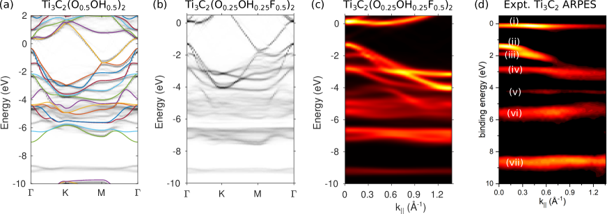
Figure 5: (a) Calculated effective band structure of Ti₃C₂(O_0.5OH_0.5)₂ overlaid with the band structure from pseudohydrogenated system. (b) Effective band structure of Ti₃C₂(O_0.25OH_0.25F_0.5)₂. (c) The same as panel (b), but showing only the $\Gamma$-K line, broadened, and colormap chosen to match that in the experiments. (d) Experimentally measured ARPES spectrum of Ti₃C₂T_x, adapted from Ref. Schultz et al., 2019.

To verify that our calculations properly capture the main features in the electronic structures of MXenes, we compare them to the only available experimental piece of information: the ARPES results for Ti₃C₂ reported in Ref. Schultz et al., 2019. The experimental data is reproduced in Fig. LABEL:arpes(d) and shows: (i) flat band at the Fermi-level, (ii) band with negative dispersion starting at -1.5 eV, (iii) band with negative dispersion starting at -2 eV, (iv) flat band at -3 eV, (v) flat band segment at -4 eV, (vi) broad flat band between -5 and -6 eV, and (vii) broad flat band between -8 and -9 eV. The composition was determined to be Ti₃C₂F_0.8O_0.8.

In Fig. 5(a) we replot the effective band structure of Ti₃C₂(O_0.5OH_0.5)₂ overlaid with the pseudohydrogenated band structure from Fig. 1(a), but in a wider energy range. As discussed, the non-bonding Ti bands at and above 0 eV and the Ti-C bonding bands between -4 and 0 eV are well reproduced in the pseudohydrogenated systems. The Ti-O bands between -7 and -4 eV are not reproduced very well, and the O-H states at -9 eV are understandably poorly described by pseudohydrogens. Also some parts of the effective band structure are more strongly smeared by the surface group disorder than others, whereas the pseudohydrogen band structures contain no disorder. These factors limit the use of the pseudohydrogenated structures for reproducing ARPES results of deeper states.

Since the features close to Fermi-level [features (i)–(iii) above] are properly described by pseudohydrogen models, we can start by comparing them to the band structures in Fig. LABEL:fig:bs. Feature (i) indicates that the non-bonding band at $\Gamma$-point must be occupied, and therefore O content must be less than about $0.25$. The gap of about 1.5 eV between features (i) and (ii) would match to the pure OH-terminated surface. We then calculated effective band structures for few different mixtures with small O content and found overall best agreement with Ti₃C₂(O_0.25OH_0.25F_0.5)₂, as shown in Fig. 5(b) and processed such that it is more comparable to the experimental spectrum in Fig. 5(c). In this case, features (i)–(iv) are all reproduced very well. The EBS also shows flat band away from the $\Gamma$-point at about -4 eV, matching well with feature (v) in the experimental spectrum. We also reproduce fairly well the broad band between -5 and -6 eV, feature (vi). The lowest energy feature (vii) is not reproduced in our calculations. The band at -7 eV in EBS originates from Ti-F bonds and the band at below -9 eV from O-H bonds. Since semilocal functionals, such as PBEsol one used here, are known to underestimate band widths and experimentally measured sample should contain significant amount of F, we ascribe feature (vii) to Ti-F bonds, in agreement with the discussion in Ref. Schultz et al., 2019.

III.4 Conclusions

In conclusion, we presented a study of the fermiology of titanium carbide and nitride MXenes via density-functional theory calculations. We first calculated the effective band structures for surfaces with mixtures of O and OH groups. The electronic structure near the Fermi-level was found to evolve gradually with the composition, and we further showed they are very well reproduced by surfaces fully terminated with pseudohydrogenated OH groups. With the pseudohydrogenated surfaces we could readily access Fermi-surface properties, such as Fermi-surface area (or length in the case of 2D materials) and Fermi-velocity. We calculated the electrical conductivity within the constant relaxation time approximation and by comparing to the experimentally determined conductivities we obtained relaxation time of about 1 fs. For the same relaxation time, the conductivities for all studied MXenes were rather similar and also fairly independent of the surface composition, changing at most by a factor of two. Finally, we compared our effective band structures to those obtained from recent ARPES experiments Schultz et al. (2019) for Ti₃C₂, where the best agreement was obtained using Ti₃C₂(O_0.25OH_0.25F_0.5)₂ model.

The approaches demonstrated here can be used also for other MXenes, including double MXenes Anasori et al. (2015) and even solid solutions in the M or X sublattice if their positions and those of the surface functional groups are uncorrelated. With the pseudohydrogenation approach it should be possible to calculate many other material properties of MXenes with an effective mixed surface composition, such as optical properties and electron-electron and electron-phonon scattering rates. It will also allow investigating how instabilities in electronic structure, leading to e.g. magnetism or charge density waves, depend on the surface composition.

References

- Naguib et al. (2012) M. Naguib, O. Mashtalir, J. Carle, V. Presser, J. Lu, L. Hultman, Y. Gogotsi, and M. W. Barsoum, ACS Nano 6, 1322 (2012), eprint http://dx.doi.org/10.1021/nn204153h, URL http://dx.doi.org/10.1021/nn204153h.
- Gogotsi and Anasori (2019) Y. Gogotsi and B. Anasori, ACS Nano 13, 8491 (2019), pMID: 31454866, eprint https://doi.org/10.1021/acsnano.9b06394, URL https://doi.org/10.1021/acsnano.9b06394.
- Naguib et al. (2011) M. Naguib, M. Kurtoglu, V. Presser, J. Lu, J. Niu, M. Heon, L. Hultman, Y. Gogotsi, and M. W. Barsoum, Advanced Materials 23, 4248 (2011), ISSN 1521-4095, URL http://dx.doi.org/10.1002/adma.201102306.
- Anasori et al. (2017) B. Anasori, M. R. Lukatskaya, and Y. Gogotsi, Nature Reviews Materials 2, 16098 (2017), URL https://www.nature.com/articles/natrevmats201698.
- Fu et al. (2019) Z. Fu, N. Wang, D. Legut, C. Si, Q. Zhang, S. Du, T. C. Germann, J. S. Francisco, and R. Zhang, Chemical Reviews 119, 11980 (2019), pMID: 31710485, eprint https://doi.org/10.1021/acs.chemrev.9b00348, URL https://doi.org/10.1021/acs.chemrev.9b00348.
- Lee and Kim (2020) E. Lee and D.-J. Kim, Journal of The Electrochemical Society 167, 037515 (2020), URL https://doi.org/10.1149%2F2.0152003jes.
- Matsuda and Hasegawa (2007) I. Matsuda and S. Hasegawa, Journal of Physics: Condensed Matter 19, 355007 (2007), URL https://doi.org/10.1088/0953-8984/19/35/355007.
- Lasek et al. (2021) K. Lasek, J. Li, S. Kolekar, P. M. Coelho, L. Guo, M. Zhang, Z. Wang, and M. Batzill, Surface Science Reports p. 100523 (2021), ISSN 0167-5729, URL https://www.sciencedirect.com/science/article/pii/S016757292100008X.
- Schultz et al. (2019) T. Schultz, N. C. Frey, K. Hantanasirisakul, S. Park, S. J. May, V. B. Shenoy, Y. Gogotsi, and N. Koch, Chemistry of Materials 31, 6590 (2019), eprint https://doi.org/10.1021/acs.chemmater.9b00414, URL https://doi.org/10.1021/acs.chemmater.9b00414.
- Chen et al. (2017) L. Chen, P. Cheng, and K. Wu, Journal of Physics: Condensed Matter 29, 103001 (2017), URL https://doi.org/10.1088/1361-648x/aa54da.
- Ouisse and Barsoum (2017) T. Ouisse and M. W. Barsoum, Materials Research Letters 5, 365 (2017), eprint https://doi.org/10.1080/21663831.2017.1333537, URL https://doi.org/10.1080/21663831.2017.1333537.
- Xie and Kent (2013) Y. Xie and P. R. C. Kent, Phys. Rev. B 87, 235441 (2013), URL http://link.aps.org/doi/10.1103/PhysRevB.87.235441.
- Khazaei et al. (2013) M. Khazaei, M. Arai, T. Sasaki, C.-Y. Chung, N. S. Venkataramanan, M. Estili, Y. Sakka, and Y. Kawazoe, Advanced Functional Materials 23, 2185 (2013), ISSN 1616-3028, URL http://dx.doi.org/10.1002/adfm.201202502.
- Khazaei et al. (2017) M. Khazaei, A. Ranjbar, M. Arai, T. Sasaki, and S. Yunoki, J. Mater. Chem. C 5, 2488 (2017), URL http://dx.doi.org/10.1039/C7TC00140A.
- Hu et al. (2015) T. Hu, H. Zhang, J. Wang, Z. Li, M. Hu, J. Tan, P. Hou, F. Li, and X. Wang, Scientific Reports 5, 16329 (2015).
- Ibragimova et al. (2019) R. Ibragimova, M. J. Puska, and H.-P. Komsa, ACS Nano 13, 9171 (2019), eprint https://doi.org/10.1021/acsnano.9b03511, URL https://doi.org/10.1021/acsnano.9b03511.
- Ibragimova et al. (2021) R. Ibragimova, P. Erhart, P. Rinke, and H.-P. Komsa, The Journal of Physical Chemistry Letters 12, 2377 (2021), eprint https://doi.org/10.1021/acs.jpclett.0c03710, URL https://doi.org/10.1021/acs.jpclett.0c03710.
- Ku et al. (2010) W. Ku, T. Berlijn, and C.-C. Lee, Phys. Rev. Lett. 104, 216401 (2010), URL https://link.aps.org/doi/10.1103/PhysRevLett.104.216401.
- Popescu and Zunger (2010) V. Popescu and A. Zunger, Phys. Rev. Lett. 104, 236403 (2010), URL https://link.aps.org/doi/10.1103/PhysRevLett.104.236403.
- Kresse and Furthmüller (1996a) G. Kresse and J. Furthmüller, Comput. Mater. Sci. 6, 15 (1996a).
- Kresse and Furthmüller (1996b) G. Kresse and J. Furthmüller, Phys. Rev. B 54, 11169 (1996b).
- Blöchl (1994) P. E. Blöchl, Phys. Rev. B 50, 17953 (1994), URL https://link.aps.org/doi/10.1103/PhysRevB.50.17953.
- Perdew et al. (2008) J. P. Perdew, A. Ruzsinszky, G. I. Csonka, O. A. Vydrov, G. E. Scuseria, L. A. Constantin, X. Zhou, and K. Burke, Phys. Rev. Lett. 100, 136406 (2008), URL https://link.aps.org/doi/10.1103/PhysRevLett.100.136406.
- Medeiros et al. (2014) P. V. C. Medeiros, S. Stafström, and J. Björk, Phys. Rev. B 89, 041407 (2014), URL https://link.aps.org/doi/10.1103/PhysRevB.89.041407.
- Madsen et al. (2018) G. K. Madsen, J. Carrete, and M. J. Verstraete, Computer Physics Communications 231, 140 (2018), ISSN 0010-4655, URL https://www.sciencedirect.com/science/article/pii/S0010465518301632.
- Ganose et al. (2021) A. M. Ganose, A. Searle, A. Jain, and S. M. Griffin, Journal of Open Source Software 6, 3089 (2021), URL https://doi.org/10.21105/joss.03089.
- Hu et al. (2017) T. Hu, Z. Li, M. Hu, J. Wang, Q. Hu, Q. Li, and X. Wang, The Journal of Physical Chemistry C 121, 19254 (2017), eprint https://doi.org/10.1021/acs.jpcc.7b05675, URL https://doi.org/10.1021/acs.jpcc.7b05675.
- Häglund et al. (1993) J. Häglund, A. Fernández Guillermet, G. Grimvall, and M. Körling, Phys. Rev. B 48, 11685 (1993), URL https://link.aps.org/doi/10.1103/PhysRevB.48.11685.
- Halim et al. (2014) J. Halim, M. R. Lukatskaya, K. M. Cook, J. Lu, C. R. Smith, L.-Å. Näslund, S. J. May, L. Hultman, Y. Gogotsi, P. Eklund, et al., Chemistry of Materials 26, 2374 (2014), pMID: 24741204, eprint https://doi.org/10.1021/cm500641a, URL https://doi.org/10.1021/cm500641a.
- Ling et al. (2014) Z. Ling, C. E. Ren, M.-Q. Zhao, J. Yang, J. M. Giammarco, J. Qiu, M. W. Barsoum, and Y. Gogotsi, Proceedings of the National Academy of Sciences 111, 16676 (2014), ISSN 0027-8424, eprint https://www.pnas.org/content/111/47/16676.full.pdf, URL https://www.pnas.org/content/111/47/16676.
- Shahzad et al. (2016) F. Shahzad, M. Alhabeb, C. B. Hatter, B. Anasori, S. Man Hong, C. M. Koo, and Y. Gogotsi, Science 353, 1137 (2016), ISSN 0036-8075, eprint https://science.sciencemag.org/content/353/6304/1137.full.pdf, URL https://science.sciencemag.org/content/353/6304/1137.
- Liu et al. (2020) J. Liu, Z. Liu, H.-B. Zhang, W. Chen, Z. Zhao, Q.-W. Wang, and Z.-Z. Yu, Advanced Electronic Materials 6, 1901094 (2020), eprint https://onlinelibrary.wiley.com/doi/pdf/10.1002/aelm.201901094, URL https://onlinelibrary.wiley.com/doi/abs/10.1002/aelm.201901094.
- Lipatov et al. (2021) A. Lipatov, A. Goad, M. J. Loes, N. S. Vorobeva, J. Abourahma, Y. Gogotsi, and A. Sinitskii, Matter 4, 1413 (2021), ISSN 2590-2385, URL https://www.sciencedirect.com/science/article/pii/S2590238521000540.
- Soundiraraju and George (2017) B. Soundiraraju and B. K. George, ACS Nano 11, 8892 (2017), pMID: 28846394, eprint http://dx.doi.org/10.1021/acsnano.7b03129, URL http://dx.doi.org/10.1021/acsnano.7b03129.
- Halim et al. (2019) J. Halim, I. Persson, E. J. Moon, P. Kühne, V. Darakchieva, P. O. Å. Persson, P. Eklund, J. Rosen, and M. W. Barsoum, Journal of Physics: Condensed Matter 31, 165301 (2019), URL https://doi.org/10.1088%2F1361-648x%2Fab00a2.
- Hart et al. (2019) J. L. Hart, K. Hantanasirisakul, A. C. Lang, B. Anasori, D. Pinto, Y. Pivak, J. T. van Omme, S. J. May, Y. Gogotsi, and M. L. Taheri, Nature Communications 10, 522 (2019).
- Urbankowski et al. (2016) P. Urbankowski, B. Anasori, T. Makaryan, D. Er, S. Kota, P. L. Walsh, M. Zhao, V. B. Shenoy, M. W. Barsoum, and Y. Gogotsi, Nanoscale 8, 11385 (2016), URL http://dx.doi.org/10.1039/C6NR02253G.
- Anasori et al. (2015) B. Anasori, Y. Xie, M. Beidaghi, J. Lu, B. C. Hosler, L. Hultman, P. R. C. Kent, Y. Gogotsi, and M. W. Barsoum, ACS Nano 9, 9507 (2015), pMID: 26208121, eprint https://doi.org/10.1021/acsnano.5b03591, URL https://doi.org/10.1021/acsnano.5b03591.