FZZ formula of boundary Liouville CFT via conformal welding

Abstract

Liouville Conformal Field Theory (LCFT) on the disk describes the conformal factor of the quantum disk, which is the natural random surface in Liouville quantum gravity with disk topology. Fateev, Zamolodchikov and Zamolodchikov (2000) proposed an explicit expression, the so-called FZZ formula, for the one-point bulk structure constant for LCFT on the disk. In this paper we give a proof of the FZZ formula in the probabilistic framework of LCFT, which represents the first step towards rigorously solving boundary LCFT using conformal bootstrap. In contrast to previous works, our proof is based on conformal welding of quantum disks and the mating-of-trees theory for Liouville quantum gravity. As a byproduct of our proof, we also obtain the exact value of the variance for the Brownian motion in the mating-of-trees theory. Our paper is an essential part of an ongoing program proving integrability results for Schramm-Loewner evolutions, LCFT, and in the mating-of-trees theory.

1 Introduction

Liouville quantum gravity (LQG) first appeared in theoretical physics in A. Polyakov’s seminal work [Pol81] where he proposed a theory of summation over the space of Riemannian metrics on a given two dimensional surface. The fundamental building block of his framework is the Liouville conformal field theory (LCFT), which describes the law of the conformal factor of the metric tensor of a surface of fixed complex structure. LCFT was first made rigorous in probability theory in the case of the Riemann sphere in [DKRV16], and then in the case of a simply connected domain with boundary in [HRV18]; see also [DRV16, Rem18, GRV19] for the case of other topologies.

On surfaces without boundary, solving Liouville theory amounts to computing the three-point function on the sphere - which is given by the DOZZ formula proposed in [DO94, ZZ96] - and arguing that correlation functions of higher order or in higher genus can be obtained from it using the conformal bootstrap method of [BPZ84]. Recently, two major breakthroughs have been achieved, namely the rigorous proof of the DOZZ formula [KRV20] and of the conformal bootstrap on the sphere [GKRV20]. A similar program can be pursued for surfaces with boundary, where the most basic correlation function is the bulk one-point function on the disk with expression given by the Fateev-Zamolodchikov-Zamolodchikov (FZZ) formula proposed in [FZZ00]. In this paper we will prove the FZZ formula, which represents the first step towards rigorously solving boundary LCFT.

Our approach is completely different from the one used in [KRV20, Rem20, RZ22] which is based on the BPZ equations and on the operator product expansion of [BPZ84]. As explained in Section 1.1, that approach has essential obstructions to proving the FZZ formula. Instead, we rely on the rich interplay between LCFT and the random geometry corresponding to LQG. In particular, we use the idea of the quantum zipper, which says that the conformal welding of two LQG type random surfaces gives a LQG type surface decorated with a Schramm Loewner evolution (SLE). Building on the original work of [She16, DMS21] and the recent work of the first and the third authors with Holden [AHS20, AHS21], we prove a new quantum zipper result and use it to obtain the FZZ formula. As an intermediate step in our proof, we also obtain the exact value of the variance of the Brownian motion in the mating-of-trees theory by Duplantier, Miller and Sheffield [DMS21].

Besides its intrinsic interest and its relevance to conformal bootstrap, the FZZ formula yields integrability results on Gaussian multiple chaos on the unit disk or upper half plane; see Section 1.3. Moreover, it is a crucial input to the paper [AS21] of the first and the third authors on the integrability of conformal loop ensemble on the sphere. We will discuss these aspects and related ongoing projects and open questions in Section 1.4, after stating our main result in Section 1.1 and summarizing the proof strategy in Section 1.2.

1.1 Boundary Liouville conformal field theory and the FZZ formula

In the physics literature LCFT is defined by a formal path integral. We work on a simply connected domain with boundary, which by conformal invariance can equivalently be the upper-half plane $\mathbb{H}$ or the unit disk $\mathbb{D}$. For almost all of this paper we will work with $\mathbb{H}=\{z\in\mathbb{C}|\mathrm{Im}(z)>0\}$ with boundary given by the real line $\mathbb{R}$. The most basic observable of Liouville theory is the correlation function of $N$ marked points in the bulk $z_{i}\in\mathbb{H}$ with associated weights $\alpha_{i}\in\mathbb{R}$ and $M$ marked points on the boundary $s_{j}\in\mathbb{R}$ with associated weights $\beta_{j}\in\mathbb{R}$. The physics path integral definition of this correlation function is then

$$\mathopen{}\mathclose{{}\left\langle\prod_{i=1}^{N}e^{\alpha_{i}\phi(z_{i})}\prod_{j=1}^{M}e^{\frac{\beta_{j}}{2}\phi(s_{j})}}\right\rangle=\int_{X:\mathbb{H}\rightarrow\mathbb{R}}DXe^{-S_{L}(X)}\mathopen{}\mathclose{{}\left(\prod_{i=1}^{N}e^{\alpha_{i}X(z_{i})}\prod_{j=1}^{M}e^{\frac{\beta_{j}}{2}X(s_{j})}}\right),$$ (1.1)

where $DX$ is a formal uniform measure over the space of all maps $X$ from the domain $\mathbb{H}$ to $\mathbb{R}$ and $S_{L}(X)$ is the so-called Liouville action which has expression given by:

$$S_{L}(X) =\frac{1}{4\pi}\int_{\mathbb{H}}\mathopen{}\mathclose{{}\left(|\partial^{g}X|^{2}+QR_{g}X+4\pi\mu e^{\gamma X}}\right)g(x)d^{2}x+\frac{1}{2\pi}\int_{\mathbb{R}}\mathopen{}\mathclose{{}\left(QK_{g}X+\mu_{B}e^{\frac{\gamma}{2}X}}\right)g(x)^{1/2}dx.$$ (1.2)

Here the background metric is $g=g(x)dx^{2}$, $R_{g}$ and $K_{g}$ are respectively the Ricci and geodesic curvatures on $\mathbb{H}$ and $\mathbb{R}$, $\gamma\in(0,2)$ is the coupling parameter for LCFT, $Q=\frac{\gamma}{2}+\frac{2}{\gamma}$ is called the background charge, and $\mu,\mu_{B}>0$ are called cosmological constants. They tune respectively the interaction strength of the Liouville potentials $e^{\gamma X}$ and $e^{\frac{\gamma}{2}X}$. Although the definition of $S_{L}(X)$ depends on a choice of background metric $g$, the correlation functions depend trivially on this choice thanks to the Weyl anomaly proved in [HRV18].

As a conformal field theory, it is well known that the (bulk) one-point correlation function $\mathopen{}\mathclose{{}\left\langle e^{\alpha\phi(z)}}\right\rangle$ of LCFT must have the following form

$$\mathopen{}\mathclose{{}\left\langle e^{\alpha\phi(z)}}\right\rangle=\frac{U(\alpha)}{\mathopen{}\mathclose{{}\left|\operatorname{Im}z}\right|^{2\Delta_{\alpha}}}\quad\textrm{ for }z\in\mathbbm{H},$$ (1.3)

where $U(\alpha)$ is called the structure constant and $\Delta_{\alpha}=\frac{\alpha}{2}(Q-\frac{\alpha}{2})$ is called the scaling dimension. In [FZZ00], the following exact formula for $U(\alpha)$ was proposed

$$U_{\mathrm{FZZ}}(\alpha):=\frac{4}{\gamma}2^{-\frac{\alpha^{2}}{2}}\mathopen{}\mathclose{{}\left(\frac{\pi\mu}{2^{\gamma\alpha}}\frac{\Gamma(\frac{\gamma^{2}}{4})}{\Gamma(1-\frac{\gamma^{2}}{4})}}\right)^{\frac{Q-\alpha}{\gamma}}\Gamma(\frac{\gamma\alpha}{2}-\frac{\gamma^{2}}{4})\Gamma(\frac{2\alpha}{\gamma}-\frac{4}{\gamma^{2}}-1)\cos((\alpha-Q)\pi s),$$ (1.4)

where the parameter $s$ is related to the ratio of cosmological constants $\frac{\mu_{B}}{\sqrt{\mu}}$ through the relation:

$$\cos\frac{\pi\gamma s}{2}=\frac{\mu_{B}}{\sqrt{\mu}}\sqrt{\sin\frac{\pi\gamma^{2}}{4}},\quad\text{with}\quad\begin{cases}s\in[0,\frac{1}{\gamma}),\quad\text{when}\quad\frac{\mu^{2}_{B}}{\mu}\sin\frac{\pi\gamma^{2}}{4}\leq 1,\\ s\in i[0,+\infty),\quad\text{when}\quad\frac{\mu^{2}_{B}}{\mu}\sin\frac{\pi\gamma^{2}}{4}\geq 1.\end{cases}$$ (1.5)

Notice $U_{\mathrm{FZZ}}(\alpha)$ depends non-trivially on $\mu,\mu_{B}$ only through the ratio $\frac{\mu_{B}}{\sqrt{\mu}}$, the dependence being encoded in the intricate relation (1.5) defining the parameter $s$.

The main result of our paper is a proof that $U(\alpha)=U_{\mathrm{FZZ}}(\alpha)$ where $U(\alpha)$ is defined in the rigorous probabilistic framework. Let us now outline the procedure of [DKRV16] adapted to the case of $\mathbb{H}$ in [HRV18] that allows to give a rigorous meaning to (1.1) and thus for $U(\alpha)$. All definitions will be precisely restated in Section 2.2. The first step is to interpret the $DX$ of (1.1) combined with the gradient squared term $|\partial^{g}X|^{2}$ of $S_{L}(X)$ as giving the law of the Gaussian Free Field (GFF). Concretely let $P_{\mathbbm{H}}$ be the probability measure corresponding to the free-boundary GFF on $\mathbbm{H}$ normalized to have average zero on the upper half unit circle $\partial\mathbbm{D}\cap\mathbbm{H}$. Define now the infinite measure $\mathrm{LF}_{\mathbbm{H}}(d\phi)$ obtained by sampling $(h,\mathbf{c})$ according to $P_{\mathbbm{H}}\times[e^{-Qc}\,dc]$ and setting $\phi(z)=h(z)-2Q\log|z|_{+}+\mathbf{c}$, where $|z|_{+}:=\max(|z|,1)$. The $\mathbf{c}$ is known as the zero mode in physics, which comes from the fact that the gradient $|\partial^{g}X|^{2}$ only defines the field up to a global constant, and one must integrate over this degree of freedom. This construction corresponds to choosing $g(x)=\max(1,|x|)^{-4}$ as the background metric in the Liouville action $S_{L}(X)$ in (1.1). The term $2Q\log|z|_{+}$ comes form the curvature terms of $S_{L}(X)$. As explained in [HRV18] and [RZ22], the choice of the background metric only affects the law of field by an explicit multiplicative constant given by the Weyl anomaly.

To make sense of the effect of $e^{\alpha\phi(z)}$, we let $\mathrm{LF}_{\mathbbm{H}}^{(\alpha,z)}=\lim_{\varepsilon\to 0}\varepsilon^{\alpha^{2}/2}e^{\alpha\phi_{\varepsilon}(z)}\mathrm{LF}_{\mathbbm{H}}(d\phi)$, where $\phi_{\varepsilon}$ is a suitable regularization at scale $\epsilon$ of $\phi$. By virtue of the Girsanov theorem, $\mathrm{LF}_{\mathbbm{H}}^{(\alpha,z)}$ can be realized as a sample from $\mathrm{LF}_{\mathbbm{H}}$ plus an $\alpha$-log singularity at $z$. Lastly to handle the Liouville potentials $e^{\gamma X}$ and $e^{\frac{\gamma}{2}X}$ present in $S_{L}(X)$, define the bulk and boundary Gaussian multiplicative chaos (GMC) measures of $\phi$ as the limits (see e.g. [Ber17, RV14]):

$$\mu_{\phi}(\mathbbm{H})=\lim_{\varepsilon\to 0}\epsilon^{\frac{\gamma^{2}}{2}}\int_{\mathbbm{H}}e^{\gamma\phi_{\epsilon}(z)}d^{2}z,\quad\text{and}\quad\nu_{\phi}(\mathbbm{R})=\lim_{\varepsilon\to 0}\epsilon^{\frac{\gamma^{2}}{4}}\int_{\mathbbm{R}}e^{\frac{\gamma}{2}\phi_{\epsilon}(z)}dz.$$ (1.6)

Now for $\gamma\in(0,2)$, $\mu,\mu_{B}>0$, set

$$\mathopen{}\mathclose{{}\left\langle e^{\alpha\phi(z)}}\right\rangle:=\mathrm{LF}_{\mathbbm{H}}^{(\alpha,z)}[e^{-\mu\mu_{\phi}(\mathbbm{H})-\mu_{B}\nu_{\phi}(\mathbbm{R})}-1],\quad\textrm{for }z\in\mathbbm{H}.$$ (1.7)

We will explain in Section 2.2 that $\mathopen{}\mathclose{{}\left|\mathopen{}\mathclose{{}\left\langle e^{\alpha\phi(z)}}\right\rangle}\right|<\infty$ when $\alpha\in(\frac{2}{\gamma},Q)$, thanks to the $-1$ in (1.7). Moreover, for $\Delta_{\alpha}=\frac{\alpha}{2}(Q-\frac{\alpha}{2})$, the quantity $\mathopen{}\mathclose{{}\left|\operatorname{Im}z}\right|^{2\Delta_{\alpha}}\mathopen{}\mathclose{{}\left\langle e^{\alpha\phi(z)}}\right\rangle$ does not depend on $z\in\mathbbm{H}$. For concreteness, we take $z=i$ and set

$$U(\alpha):=\mathopen{}\mathclose{{}\left\langle e^{\alpha\phi(i)}}\right\rangle.$$ (1.8)

Now we are ready to state our main result.

Theorem 1.1.

For $\gamma\in(0,2)$, $\alpha\in(\frac{2}{\gamma},Q)$, $\mu,\mu_{B}>0$, we have $U(\alpha)=U_{\mathrm{FZZ}}(\alpha)$.

The condition $\alpha\in(\frac{2}{\gamma},Q)$ is required for (1.7) to be finite, but one can extend the probabilistic definition of $U(\alpha)$ and the result to $\alpha\in(\frac{\gamma}{2},Q)$; see Theorem 1.2 and Corollary 4.19. So far in the probability literature the exact formulas on LCFT have all been derived by implementing the BPZ equations and the operator product expansion of [BPZ84], as first performed in [KRV20] proving the DOZZ formula. In the setup of a domain with boundary the same technique has been applied in the works [Rem20, RZ20, RZ22], which all compute different cases of boundary Liouville correlations with $\mu=0,\mu_{B}>0$. This method has a major obstruction to prove Theorem 1.1. Indeed, in order to define an observable satisfying the BPZ equation, the range of $\alpha$ needs to contain an interval of length strictly greater than $\frac{2}{\gamma}$. The best range of $\alpha$ for a GMC definition of $\mathopen{}\mathclose{{}\left\langle e^{\alpha\phi(z)}}\right\rangle$ is $(\frac{\gamma}{2},Q)$ - see Corollary 4.19 - which has length exactly $\frac{2}{\gamma}$ and thus is not sufficient. Another less fundamental but technically challenging issue is to reveal the intricate dependence on $\mu,\mu_{B}$ in $U_{\mathrm{FZZ}}(\alpha)$. In the next subsection, we explain our strategy based on the conformal welding of quantum surfaces that circumvents these difficulties.

1.2 A proof strategy based on the conformal welding of quantum surfaces

By definition, the FZZ formula describes the joint law of $\nu_{\phi}(\mathbbm{R})$ and $\mu_{\phi}(\mathbbm{H})$ in (1.6) where $\phi$ is a sample from $\mathrm{LF}_{\mathbbm{H}}^{(\alpha,i)}$. Here although $\mathrm{LF}_{\mathbbm{H}}^{(\alpha,i)}$ is an infinite measure we adopt the probability terminology such as “sample” and “law”. The law of $\nu_{\phi}(\mathbbm{R})$ is encoded in the limiting case of the FZZ formula where $\mu=0$ and $\mu_{B}>0$, which has been obtained in [Rem20]. Given this result, it turns out that the FZZ formula is equivalent to the statement that conditioning on $\nu_{\phi}(\mathbbm{R})=1$, the conditional law of $\mu_{\phi}(\mathbbm{H})$ is the inverse gamma distribution with certain parameters. Here the inverse gamma distribution with shape parameter $a$ and scale parameter $b$ has the following density: $1_{x>0}\frac{b^{a}}{\Gamma(a)}\frac{1}{x^{a+1}}e^{-b/x}$. The crux of this paper is to derive the desired inverse gamma distribution using conformal welding of quantum surfaces. In this section we sketch this strategy.

Quantum surfaces are the generalization of 2D Riemannian manifolds in the LQG random geometry. For a fixed $\gamma\in(0,2)$, consider triples $(D,h,z)$ where $D$ is a domain, $h$ is a variant of Gaussian free field on $D$, and $z\in D$. We say that $(D,h,z)$ is equivalent to $(\widetilde{D},\widetilde{h},\widetilde{z})$ if there exists a conformal map $\psi:\widetilde{D}\to D$ such that $\widetilde{h}=h\circ\psi+Q\log|\psi^{\prime}|$ and $\psi(z)=\widetilde{z}$. Under this equivalence relation, the intrinsic geometric quantities in $\gamma$-LQG such as the quantum area and length measures transform covariantly under conformal maps. Here the quantum area and length are defined by Gaussian multiplicative chaos as in (1.6). A quantum surface with one interior marked point is an equivalence class under this equivalence relation. We can similarly define quantum surfaces with more marked points or decorated with other natural structures such as curves.

For $\alpha\in(\frac{\gamma}{2},Q)$, sample $\phi$ from $\mathrm{LF}_{\mathbbm{H}}^{(\alpha,i)}$ and condition on $\nu_{\phi}(\mathbbm{R})=\ell>0$. (This conditioning makes sense; see Lemma 4.4.) We write the conditional law of the quantum surface corresponding to $(\mathbbm{H},\phi,i)$ as $\mathcal{M}_{1,0}^{\mathrm{disk}}(\alpha;\ell)^{\#}$. With this notion, the FZZ formula can be reduced to the following.

Theorem 1.2.

For $\alpha\in(\frac{\gamma}{2},Q)$ the law of the quantum area of a sample from $\mathcal{M}_{1,0}^{\mathrm{disk}}(\alpha;1)^{\#}$ is the inverse gamma distribution with shape $\frac{2}{\gamma}(Q-\alpha)$ and scale $\frac{1}{4\sin\frac{\pi\gamma^{2}}{4}}$.

When $\alpha=\gamma$, by [Cer21] and [AHS21], $\mathcal{M}_{1,0}^{\mathrm{disk}}(\alpha;1)^{\#}$ describes the law of the so-called quantum disk with unit boundary length and one interior marked point. In this case, based on the mating-of-trees theory of Duplantier, Miller, and Sheffield [DMS21], Gwynne and the first author of this paper [AG21] proved that the law of the quantum area is the inverse gamma distribution with shape $\frac{2}{\gamma}(Q-\gamma)$ and scale $\frac{1}{2\mathbbm{a}^{2}\sin^{2}(\pi\gamma^{2}/4)}$, where $\mathbbm{a}^{2}$ is the unknown variance in the mating-of-trees theory, which first appeared in [DMS21, Theorem 8.1].

Let us review the mating-of-trees theory. In our proofs we will only use some of its consequences that can be stated without explicit reference to it. Hence we will keep our discussion brief and refer to the survey [GHS19] for more background, especially on its fundamental role in the recent development on the scaling limit of random planar maps. Recall that the Schramm-Loewner evolution ($\operatorname{SLE}_{\kappa}$) with a parameter $\kappa>0$ is a canonical family of conformal invariant random planar curves discovered by Schramm [Sch00]. In a nutshell, mating-of-trees theory says that if we run a space-filling variant of an $\operatorname{SLE}_{16/\gamma^{2}}$ curve on top of an independent $\gamma$-LQG surface, then this curve-decorated quantum surface can be encoded by a two-dimensional correlated Brownian motion $(L_{t},R_{t})$ such that

$$\operatorname{Var}[L_{1}]=\operatorname{Var}[R_{1}]=\mathbbm{a}^{2}\textrm{ and }\operatorname{Cov}(L_{1}R_{1})=-\mathbbm{a}^{2}\cos(\frac{\gamma^{2}\pi}{4}).$$ (1.9)

Here the mating-of-trees variance $\mathbbm{a}^{2}$ is an unknown function of the parameter $\gamma$. As a first step towards proving Theorem 1.2, we identify the value of $\mathbbm{a}^{2}$.

Theorem 1.3.

For $\gamma\in(0,2)$, the mating-of-trees variance $\mathbbm{a}^{2}=\mathbbm{a}^{2}(\gamma)$ is given by

$$\mathbbm{a}^{2}=\frac{2}{\sin(\frac{\pi\gamma^{2}}{4})}.$$

We will prove Theorem 1.3 in Section 3. Our proof has two ingredients: a systematic understanding of the relation between canonical quantum surfaces and LCFT developed by the first and the third authors with Holden in [AHS21]; the explicit boundary LCFT correlation functions computed by the second author in [Rem20] and in his joint work  [RZ22] with Zhu.

To prove Theorem 1.2, we use the idea of conformal welding which we recall now. For $\gamma\in(0,2)$ and $\kappa=\gamma^{2}\in(0,4)$, if we run an independent $\operatorname{SLE}_{\kappa}$ on top of a certain type of $\gamma$-LQG quantum surface, the two quantum surfaces on the two sides of the SLE curve are independent quantum surfaces. Quantum boundary lengths from the two sides agree on the curve, defining an unambiguous notion of quantum length on the SLE curve. Moreover, the original curve-decorated quantum surface can be recovered by gluing the two smaller quantum surfaces according to the quantum boundary lengths. This recovering procedure is called conformal welding. Such results were first established by Sheffield [She16] and later extended in [DMS21, AHS20].

In this paper we prove a new conformal welding result that enables us to derive the inverse gamma distribution in Theorem 1.2. It asserts the existence of an $\operatorname{SLE}_{\kappa}$ type curve $\eta$ with the following properties. See Figure 1 for an illustration.

• $\eta$ is a simple closed random curve surrounding $i$ that visits 0 and otherwise is in $\mathbbm{H}$.

• Suppose $\phi$ is independent of $\eta$ and is sampled from the conditional law of $\mathrm{LF}^{(\alpha,i)}_{\mathbbm{H}}$ conditioning on $\nu_{\phi}(\mathbbm{R})=1$. Let $D_{\eta}(0)$ and $D_{\eta}(\infty)$ be the bounded and unbounded component of $\mathbbm{H}\setminus\eta$, respectively. Then as quantum surfaces with marked points, $(D_{\eta}(0),\phi,i,0)$ and $(D_{\eta}(\infty),\phi,0^{-},0^{+})$ are conditionally independent given the quantum length of $\eta$.

• The conditional law of $(D_{\eta}(0),\phi,i)$ conditioning on the quantum length $\ell$ of $\eta$ is $\mathcal{M}_{1,0}^{\mathrm{disk}}(\alpha;\ell)^{\#}$.

• The law of the quantum area and quantum lengths of the two boundary arcs of $(D_{\eta}(\infty),\phi,0^{-},0^{+})$ can be explicitly described in terms of the mating-of-trees Brownian motion $(L_{t},R_{t})$.

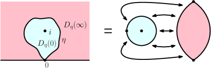
Figure 1: Left: A curve $\eta$ independent of a sample $\phi$ from $\mathrm{LF}_{\mathbbm{H}}^{(\alpha,i)}$. Right: The quantum surfaces $(D_{\eta}(0),\phi,i,0)$ and $(D_{\eta}(\infty),\phi,0^{-},0^{+})$ are conditionally independent given the quantum length of $\eta$. Moreover, $(\phi,\eta)$ can be recovered from the two quantum surfaces by conformal welding.

This result is stated as Theorem 4.6 and proved in Sections 4.2 and 5. It relies on the conformal welding results for finite area quantum surfaces proved in [AHS20]. The law of $(D_{\eta}(\infty),\phi,0^{-},0^{+})$ is given by a variant of the so-called two-pointed quantum disk with weight $\gamma^{2}/2$, whose quantum length and area distribution is obtained in [AHS20] in terms of the mating-of-trees Brownian motion; see Section 2.5.

Using the above conformal welding result, we can obtain a recursive relation on the law of the quantum area of a sample from $\mathcal{M}_{1,0}^{\mathrm{disk}}(\alpha;1)^{\#}$. Using a path decomposition for Brownian motion in cones, we prove that the only solution to this recursion is the inverse gamma distribution in Theorem 1.2, which is identified as the law of the duration of a certain Brownian motion in cones. For technical reasons, we carry out this argument for $\alpha\in(\frac{\gamma}{2},Q-\frac{\gamma}{4})$ first. This gives Theorem 1.1 for $\alpha\in(\frac{2}{\gamma},Q-\frac{\gamma}{4})$. Since $\frac{\gamma}{2}<\frac{2}{\gamma}<Q-\frac{\gamma}{4}$, by the analyticity of $U(\alpha)$ in $\alpha\in(\frac{2}{\gamma},Q)$, we obtain Theorem 1.1 in its full range $(\frac{2}{\gamma},Q)$, which in turn gives Theorem 1.2 in its full range $(\frac{\gamma}{2},Q)$. It also allows us to extend Theorem 1.1 to $\alpha\in(\frac{\gamma}{2},Q)$ for a suitably defined $U(\alpha)$; see Corollary 4.19. See Section 4 for the detailed argument.

1.3 Exact solvability for moments of a Gaussian multiplicative chaos

It is natural to look at the limits $\mu\rightarrow 0$ or $\mu_{B}\rightarrow 0$ in the exact formula of Theorem 1.1. These limits have the effect of deleting one of the two Liouville potentials in (1.2) and the probabilistic expression for $U(\alpha)$ then reduces up to an explicit prefactor to a moment of GMC either on the bulk or on the boundary of the domain. In the case of $\mu\rightarrow 0$, see equation (2.5) for this reduction. Our main result then reduces in this case to Proposition 2.8 giving an exact formula for the moment of GMC on $\mathbb{R}$. This formula was derived in [Rem20] and is actually used in our proof of Theorem 1.1. On the other hand the limit $\mu_{B}\rightarrow 0$ provides a novel result on the moments of GMC on $\mathbb{H}$.

Proposition 1.4.

Let $\gamma\in(0,2)$, $\alpha\in(\frac{\gamma}{2},Q)$, and $\widetilde{\phi}=h-2Q\log|z|_{+}+\alpha G_{\mathbb{H}}(z,i)$, where $h$ is a sample from $P_{\mathbb{H}}$. Then

$$\mathbbm{E}\mathopen{}\mathclose{{}\left[\mu_{\widetilde{\phi}}(\mathbb{H})^{\frac{1}{\gamma}(Q-\alpha)}}\right]=\frac{2}{\sqrt{\pi}}\mathopen{}\mathclose{{}\left(\frac{\pi}{2^{\gamma\alpha+2}}\frac{\Gamma(\frac{\gamma^{2}}{4})}{\Gamma(1-\frac{\gamma^{2}}{4})}}\right)^{\frac{Q-\alpha}{\gamma}}\Gamma(\frac{\gamma\alpha}{2}-\frac{\gamma^{2}}{4})\Gamma(\frac{\alpha}{\gamma}-\frac{2}{\gamma^{2}})\cos\mathopen{}\mathclose{{}\left(\pi\frac{\alpha-Q}{\gamma}}\right).$$ (1.10)

A further corollary can be derived if one assumes the moment $\frac{1}{\gamma}(Q-\alpha)$ of the above GMC to be an integer $n\in\mathbb{N}$. It is a well-known simple Gaussian computation that a positive integer moment of GMC reduces to a Selberg type integral, see [FW08] for a review on these integrals.

Corollary 1.5.

Let $\gamma\in(0,2)$ and $n\in\mathbb{N}$ such that $0<n<\frac{2}{\gamma^{2}}$. Then the following holds:

$$\int_{\mathbb{H}^{n}}dz_{1}\cdots dz_{n}\prod_{i<j}\mathopen{}\mathclose{{}\left(\frac{1}{|z_{i}-z_{j}|^{\gamma^{2}}|z_{i}-\overline{z}_{j}|^{\gamma^{2}}}}\right)\prod_{i=1}^{n}\mathopen{}\mathclose{{}\left(\frac{1}{|z_{i}-\overline{z}_{i}|^{\frac{\gamma^{2}}{2}}}\frac{1}{|z_{i}^{2}+1|^{\gamma Q-n\gamma^{2}}}}\right)$$ (1.11)

$$\quad=\frac{2}{\sqrt{\pi}}\mathopen{}\mathclose{{}\left(\frac{-\pi}{2^{4+\frac{\gamma^{2}}{2}(1-2n)}}\frac{\Gamma(\frac{\gamma^{2}}{4})}{\Gamma(1-\frac{\gamma^{2}}{4})}}\right)^{n}\Gamma(1-\frac{\gamma^{2}}{2}n)\Gamma(\frac{1}{2}-n).$$

The integral (1.11) ressembles the Dotsenko-Fateev integral of [DF84] appearing in the context of CFT on the Riemann sphere, with $\mathbb{C}^{n}$ being replaced by $\mathbb{H}^{n}$. To the best of our knowledge the above evaluation of (1.11) was not known. Notice that for $\gamma\geq\sqrt{2}$, there are no valid $n$ as the first moment of the GMC on $\mathbb{H}$ is not finite. For any $\gamma\in(0,\sqrt{2})$, there are finitely many $n$ that satisfy $0<n<\frac{2}{\gamma^{2}}$. Lastly let us note by conformal invariance it is possible to write both of these results on the unit disk $\mathbb{D}$, see for instance [RZ22, Section 5.3] for how to link moments of GMC on $\mathbb{D}$ and $\mathbb{H}$.

1.4 Perspectives and outlook

In this section we describe several perspectives, ongoing projects, and future directions related to the FZZ formula.

1.4.1 Integrability and the conformal bootstrap for boundary LCFT

In order to carry out the conformal bootstrap for LCFT on Riemann surfaces with boundary, along with the bulk one-point function that we obtained in Thoerem 1.1, one needs to compute three other correlation functions for LCFT on $\mathbbm{H}$

$$\mathopen{}\mathclose{{}\left\langle e^{\alpha\phi(z)}e^{\frac{\beta}{2}\phi(s)}}\right\rangle,\quad\mathopen{}\mathclose{{}\left\langle e^{\frac{\beta}{2}\phi(s_{1})}e^{\frac{\beta}{2}\phi(s_{2})}}\right\rangle,\quad\mathopen{}\mathclose{{}\left\langle e^{\frac{\beta_{1}}{2}\phi(s_{1})}e^{\frac{\beta_{2}}{2}\phi(s_{2})}e^{\frac{\beta_{3}}{2}\phi(s_{3})}}\right\rangle,$$ (1.12)

where $z\in\mathbb{H}$, $s,s_{1},s_{2},s_{3}\in\mathbb{R}$. For the boundary two-point and three-point functions one also has the freedom to choose $\mu_{B}$ as a function defined on the boundary which is constant on each arc in between boundary insertions. See [RZ22, Figure 1] for a summary.

Along with $\mathopen{}\mathclose{{}\left\langle e^{\alpha\phi(z)}}\right\rangle$, these three correlation functions are the “basic” correlations as thanks to conformal invariance they depend trivially on $z,s_{1},s_{2},s_{3}$. On the other hand their dependence on $\gamma,\mu,\mu_{B},\alpha,\beta,\beta_{i}$ is non-trivial. Explicit formulas for these functions have been proposed in the physics papers [FZZ00, Hos01, PT02]. In the limiting case where $\mu=0$, they reduce to moments of the boundary GMC measure and they have been explicitly computed in the work [RZ22]. In a work in progress with Zhu, we plan to verify the proposed formulas for all three correlations for general $\mu>0$. The techniques will be a combination of the tools of the present paper and of [RZ22]. Indeed, the approach in [RZ22] is still applicable to the second and third correlation functions in (1.12) as there is no bulk insertion. By a conformal welding statement similar to the one in this paper, we will get the first one from the second one and the FZZ formula.

Once the above correlations have been evaluated, the next natural step is to compute a correlation function with more marked points or on a non simply connected surface with boundary. For this purpose one needs to implement the conformal bootstrap procedure first proposed in physics in [BPZ84]. At the level of mathematics this has been achieved to compute an $N$-point function on the sphere in the recent breakthrough [GKRV20]. One can expect to adapt the methods of [GKRV20] to the case of a surface with boundary, where the FZZ formula along with the correlations (1.12) are a crucial input. More concretely in [Mar03] a bootstrap equation involving the FZZ formula is proposed to compute the partition function of LCFT on an annulus. We state it here as a conjecture.

Conjecture 1.6.

Consider an annulus represented as a cylinder of length $\pi\tau$ and of radius $1$. Let $q=e^{-2\pi\tau}$ and $\mathcal{Z}_{\mathrm{Annulus}}$ be the partition function (no insertion points) of LCFT on this annulus defined probabilistically in an analogous way to (1.7), see also [Rem18]. Then the following equality should hold:

$$\mathcal{Z}_{\mathrm{Annulus}}=\int_{\mathcal{C}}U_{\mathrm{FZZ}}(Q+iP)U_{\mathrm{FZZ}}(Q-iP)q^{P^{2}-\frac{1}{24}}\prod_{n\geq 1}(1-q^{n})dP.$$ (1.13)

One has the degree of freedom to choose different values of $\mu_{B}$ for each of the two boundaries of the annulus, in which case the two $U_{\mathrm{FZZ}}$ functions in the right hand side of (1.13) must be computed respectively with those two values. The $\mu$ parameter is the same for $\mathcal{Z}_{\mathrm{Annulus}}$ and both $U_{\mathrm{FZZ}}$ functions. Lastly the contour of integration $\mathcal{C}$ is a suitable deformation of $\mathbb{R}$ avoiding the pole at $P=0$.

1.4.2 Interplay between three types of integrability in conformal probability

Our paper is part of an ongoing program of the first and the third authors to prove integrable results for SLE, LCFT, and mating-of-trees via two connections between these subjects: 1. equivalent but complementary descriptions of canonical random surfaces in the path integral (e.g. [DKRV16]) and mating-of-trees (e.g. [DMS21]) perspectives; 2. conformal welding of these surfaces with SLE curves as the interface. We now describe other aspects in this program that are closely related to this paper.

• Our paper relies on the recent work of the first and the third authors with Holden [AHS20, AHS21]. In particular, our conformal welding result is built on the one proved in [AHS20] for two-pointed quantum disks. Our evaluation of the mating-of-trees variance uses the technique from [AHS21] on the LCFT description of quantum surfaces.

  One of the main results in [AHS21] is an exact formula for a variant of SLE curves called the chordal $\operatorname{SLE}_{\kappa}(\rho_{-};\rho_{+})$ (see Section 2.4). Its proof shares the same starting point with our proof of the FZZ formula: a conformal welding result for quantum disks.

  [AHS21] demonstrated how to get integrability results for SLE using LCFT, mating-of-trees and conformal welding. Using the same methodology and taking the FZZ formula as a crucial input, the first and the third authors proved two integrable results on the conformal loop ensemble in [AS21]. The first relates the three-point correlation function of the conformal loop ensemble on the sphere  [IJS16] with the DOZZ formula. The other addresses a conjecture of Kenyon and Wilson (recorded in [SSW09, Section 4]) on its electrical thickness.

• Our proof of the FZZ formula does not rely on conformal field theoretical techniques such as the BPZ equations and operator product expansion, except for two exact formulas from [Rem20] and [RZ22]; see (2.6) and (3.4). In an ongoing project with Da Wu, the first and the third authors aim at using the conformal welding and stochastic calculus methods in SLE to recover these two formulas. Combined with our paper, this will provide a proof of the FZZ formula which is fully based on SLE, mating-of-trees, and conformal welding. It is an interesting open question whether such a proof can be given for the DOZZ formula.

• The first and the third authors are working on verifying our belief that in a very general sense the conformal welding of two quantum surfaces defined by LCFT can be described by LCFT, where the conformal welding result (Theorem 4.1) in this paper is a special case. For another instance of this statement, consider a pair of independent Liouville fields on a disk with three boundary insertions. If we conformally weld them along the three boundary arcs, then the resulting surface should be given by a Liouville field on the sphere with three bulk insertions. Moreover, the magnitude of an insertion on the sphere is determined by the local rule for conformal welding described in [DMS21]. More precisely, in the terminology of [DMS21], if we zoom in around an insertion on the sphere the picture looks like the conformal welding of two quantum wedges into a quantum cone, which is understood in [DMS21]. In our present case, if we zoom in around $0$ in Figure 1, the picture will converge to the conformal welding of three quantum wedges into a single quantum wedge as established in [DMS21].

1.4.3 FZZT branes and related models

We review here several models related to the FZZ formula in the theoretical physics literature. Boundary Liouville theory admits two kinds of boundary states, the one studied in the present paper being the so-called Fateev-Zamolodchikov-Zamolodchikov-Teschner (FZZT) brane [FZZ00], [Tes00]. The other is the Zamolodchikov-Zamolodchikov (ZZ) brane which corresponds to LCFT on a disk with the hyperbolic metric as background metric; see [ZZ01]. In this ZZ brane setup there is also a formula for the bulk one-point function, see [ZZ01, Equation (2.16)]. Both the FZZT and ZZ branes play a role in the relation between matrix models, integrable heirarchies, and Liouville quantum gravity; see for instance [AB19] and references therein. Lastly one can consider LCFT on a non-orientable surface, the simplest model being the projective plane, see [Hik03, Equation (3.10)] for the analogue of $U(\alpha)$ in that case. We hope to adapt our methods to study these directions in the future, see also the review [Nak04] for more details.

Organization of the paper. After providing background in Section 2, we obtain the mating of trees variance in Section 3. Then in Section 4, we carry out the strategy outlined in Section 1.2 modulo the proof of the conformal welding result, whose proof is supplied in Section 5.

Acknowledgements. We thank Nina Holden, Rémi Rhodes, Vincent Vargas, and Tunan Zhu for early discussions on alternative approaches towards proving the FZZ formula. We also thank Scott Sheffield for suggesting the mating-of-trees variance problem and Ewain Gwynne for helpful discussions on this. We thank Konstantin Aleshkin for many explanations on the theoretical physics background behind the FZZ formula. We are grateful to Wendelin Werner for enlightening discussions. We thank an anonymous referee for helpful comments on an earlier version of this paper. This project was initiated when G.R. visited MIT in the Spring of 2018. He would like to very warmly thank Scott Sheffield for his hospitality. M.A. was partially supported by NSF grant DMS-1712862. G.R. was supported by an NSF mathematical sciences postdoctoral research fellowship, NSF Grant DMS-1902804. X.S. was supported by the Simons Foundation as a Junior Fellow at the Simons Society of Fellows, and by the NSF grant DMS-2027986 and the Career award 2046514.

2 Preliminaries

In this section we provide the necessary background for our proofs. We start by fixing some global notations and conventions in Section 2.1. We then review Liouville CFT and quantum disks in Section 2.2 and 2.3, respectively. We will only need these two sections for the evaluation of the mating of trees variance in Section 3. We recall the conformal welding of quantum disks in Section 2.4 and some properties on two special quantum disks in Section 2.5.

2.1 Notations and conventions

Throughout the paper we assume $\gamma\in(0,2)$ is the LQG coupling constant. Moreover,

$$Q=\frac{\gamma}{2}+\frac{2}{\gamma}\quad\textrm{and}\quad\kappa=\gamma^{2}.$$ (2.1)

We will work with planar domains including the upper half plane $\mathbbm{H}=\{z\in\mathbbm{C}:\operatorname{Im}(z)>0\}$, the unit disk $\mathbbm{D}=\{z\in\mathbbm{C}:|z|<1\}$, and the horizontal strip $\mathcal{S}=\mathbbm{R}\times(0,\pi)$. For a domain $D\subset\mathbbm{C}$, we write $\partial D$ of $D$ as the set of prime ends of $D$ and call it the boundary of $D$. For example, $\partial\mathbbm{H}=\mathbbm{R}\cup\{\infty\}$ and $\partial\mathcal{S}=\{z\in\mathbbm{C}:\operatorname{Im}z=0\textrm{ or }1\}\cup\{\pm\infty\}$.

We write $\Gamma$ as the unique meromorphic function such that $\Gamma(\alpha)=\int_{0}^{\infty}x^{\alpha-1}e^{-x}dx$ for $\alpha>0$. For $a>0$ and $b>0$, the inverse gamma distribution with shape parameter $a$ and scale parameter $b$ has the following density:

$$1_{x>0}\frac{b^{a}}{\Gamma(a)}\frac{1}{x^{a+1}}e^{-b/x}.$$ (2.2)

We will frequently consider non-probability measures and extend the terminology of probability theory to this setting. In particular, suppose $M$ is a measure on a measurable space $(\Omega,\mathcal{F})$ such that $M(\Omega)$ is not necessarily $1$, and $X$ is a $\mathcal{F}$-measurable function. Then we say that $(\Omega,\mathcal{F})$ is a sample space, $X$ is a random variable. We call the pushforward measure $M_{X}=X_{*}M$ the law of $X$. We say that $X$ is sampled from $M_{X}$. We also write $\int f(x)M_{X}(dx)$ as $M_{X}[f]$ for simplicity. For a finite positive measure $M$, we denote as its total mass by $|M|$ and write $M^{\#}=|M|^{-1}M$ as the corresponding probability measure.

Let $g$ be a smooth metric on $\mathbbm{H}$ such that the metric completion of $(\mathbbm{H},g)$ is a compact Riemannian manifold. Let $H^{1}(\mathbbm{H},g)$ be the Sobolev space whose norm is the sum of the Dirichlet energy and the $L^{2}$-norm with respect to $(\mathbbm{H},g)$. Let $H^{-1}(\mathbbm{H})$ be the dual space of $H^{1}(\mathbbm{H},g)$. Then the function space $H^{-1}(\mathbbm{H})$ and its topology do not depend on the choice of $g$, and it is a Polish (i.e. complete separable metric) space. All random functions on $\mathbbm{H}$ considered in this paper will belong to $H^{-1}(\mathbbm{H})$.

2.2 Liouville conformal field theory on the upper half plane

For convenience we present LCFT on domains conformally equivalent to a unit disk, with the upper half plane $\mathbbm{H}$ as our base domain. Let $h$ be the centered Gaussian process on $\mathbbm{H}$ with covariance kernel given by

$$\mathbbm{E}[h(x)h(y)]=G_{\mathbbm{H}}(x,y):=\log\frac{1}{|x-y||x-\bar{y}|}+2\log|x|_{+}+2\log|y|_{+},$$ (2.3)

where $|x|_{+}:=\max(|x|,1)$ and in the sense that $\mathbbm{E}[(h,f)(h,g)]=\iint f(x)\mathbbm{E}[h(x)h(y)]g(y)dxdy$, for smooth test functions $f,g$. Let $P_{\mathbbm{H}}$ be the law of $h$. Using the arguments in [She07, Dub09] it can be shown that $P_{\mathbbm{H}}$ is a probability measure on the space $H^{-1}(\mathbbm{H})$ defined in Section 2.1. For smooth test functions $g$ and $f$ such that $\int_{\mathbbm{H}}f(z)\,d^{2}z=\int_{\mathbbm{H}}g(z)\,d^{2}z=0$, we have $\mathbbm{E}[(h,f)(h,g)]=(2\pi)^{-1}\int_{\mathbbm{H}}\nabla g\cdot\nabla f\,d^{2}z$. This is the characterizing property of the free boundary Gaussian free field, which is only uniquely defined modulo additive constant. The field $h$ is the particular variant where the additive constant is fixed by requiring the average around the upper half unit circle to be 0.

Given a function $f\in H^{-1}(\mathbbm{H})$ and $z\in\mathbbm{H}\cup\mathbbm{R}$, let $f_{\varepsilon}(z)$ be the average of $f$ over $\partial B_{\varepsilon}(z)\cap\mathbbm{H}$. For $h\sim P_{\mathbbm{H}}$, define the random measures $\mu_{h}=\lim_{\varepsilon\to 0}\varepsilon^{\gamma^{2}/2}e^{\gamma h_{\varepsilon}}d^{2}z$ and $\nu_{h}=\lim_{\varepsilon\to 0}\varepsilon^{\gamma^{2}/4}e^{\gamma h_{\varepsilon}/2}dz$, where the convergence holds in probability in weak topology. See [Ber17, RV14] and references therein for more details on this construction. We call $\mu_{h}$ and $\nu_{h}$ the quantum area and quantum boundary length measures, respectively, corresponding to $\phi$. For functions which can be written as a sum of the GFF and a continuous function, quantum length and area can be defined similarly.

Definition 2.1 (Liouville field).

Sample $(h,\mathbf{c})$ from the measure $P_{\mathbbm{H}}\times[e^{-Qc}\,dc]$ on $H^{-1}(\mathbbm{H})\times\mathbbm{R}$, and let $\phi(z)=h(z)-2Q\log|z|_{+}+\mathbf{c}$ be a random field on $\mathbbm{H}$. Let $\mathrm{LF}_{\mathbbm{H}}$ be the measure on $H^{-1}(\mathbbm{H})$ which describes the law of $\phi$. We call a sample from $\mathrm{LF}_{\mathbbm{H}}$ a Liouville field on $\mathbbm{H}$.

The following lemma defines Liouville fields with insertions by making sense of $e^{\alpha\phi(z_{0})}\mathrm{LF}_{\mathbbm{H}}(d\phi)$.

Lemma 2.2.

For $\alpha\in\mathbbm{R}$ and $z_{0}\in\mathbbm{H}$, the limit $\mathrm{LF}_{\mathbbm{H}}^{(\alpha,z_{0})}:=\lim_{\varepsilon\to 0}\varepsilon^{\alpha^{2}/2}e^{\alpha\phi_{\varepsilon}(z_{0})}\mathrm{LF}_{\mathbbm{H}}(d\phi)$ exists in the vague topology. Moreover, sample $(h,\mathbf{c})$ from $(2\operatorname{Im}z_{0})^{-\alpha^{2}/2}|z_{0}|_{+}^{-2\alpha(Q-\alpha)}P_{\mathbbm{H}}\times[e^{(\alpha-Q)c}dc]$ and let

$$\phi(z)=h(z)-2Q\log|z|_{+}+\alpha G_{\mathbbm{H}}(z,z_{0})+\mathbf{c}\quad\textrm{for }z\in\mathbbm{H}.$$

Then the law of $\phi$ is given by $\mathrm{LF}_{\mathbbm{H}}^{(\alpha,z_{0})}$.

Proof.

Sample $h$ from $P_{\mathbbm{H}}$, fix $c\in\mathbbm{R}$ and set $\widetilde{\phi}(z)=h(z)-2Q\log|z|_{+}+c$. For a compactly supported continuous function $F$ on $H^{-1}(\mathbbm{H})\times\mathbb{R}$, Girsanov’s theorem and $\operatorname{Var}h_{\varepsilon}(z_{0})=-\log\varepsilon-\log(2\operatorname{Im}z_{0})+4\log|z_{0}|_{+}+o_{\varepsilon}(1)$ give

$$\lim_{\varepsilon\to 0}\mathbbm{E}\mathopen{}\mathclose{{}\left[\varepsilon^{\alpha^{2}/2}e^{\alpha\widetilde{\phi}_{\varepsilon}(z_{0})}F(h,c)}\right] =(2\operatorname{Im}z_{0})^{-\alpha^{2}/2}|z_{0}|_{+}^{-2\alpha(Q-\alpha)}\lim_{\varepsilon\to 0}\mathbbm{E}\mathopen{}\mathclose{{}\left[e^{\alpha c}e^{\alpha h_{\varepsilon}(z_{0})-\frac{\alpha^{2}}{2}\mathbbm{E}[h_{\varepsilon}(z_{0})^{2}]}F(h,c)}\right]$$

$$=(2\operatorname{Im}z_{0})^{-\alpha^{2}/2}|z_{0}|_{+}^{-2\alpha(Q-\alpha)}\lim_{\varepsilon\to 0}\mathbbm{E}\mathopen{}\mathclose{{}\left[e^{\alpha c}F\mathopen{}\mathclose{{}\left(h(\cdot)+\alpha\mathbbm{E}[h(\cdot)h_{\varepsilon}(i)],c}\right)}\right]$$

$$=(2\operatorname{Im}z_{0})^{-\alpha^{2}/2}|z_{0}|_{+}^{-2\alpha(Q-\alpha)}\mathbbm{E}\mathopen{}\mathclose{{}\left[e^{\alpha c}F\mathopen{}\mathclose{{}\left(h(\cdot)+\alpha G_{\mathbbm{H}}(\cdot,i),c}\right)}\right].$$

Integrating over $[e^{-Qc}dc]$ yields the lemma. ∎

Definition 2.3.

We call a sample from $\mathrm{LF}_{\mathbbm{H}}^{(\alpha,z)}$ a Liouville field on $\mathbbm{H}$ with an $\alpha$-insertion at $z$.

The following lemma gives the change of coordinate for the Liouville field under a conformal map.

Lemma 2.4.

For $(\alpha,z_{0})\in\mathbbm{R}\times\mathbbm{H}$, let $\psi:\mathbbm{H}\to\mathbbm{H}$ be a conformal map such that $\psi(z_{0})=i$. Sample $\phi$ from $\mathrm{LF}_{\mathbbm{H}}^{(\alpha,z_{0})}$, then the law of $\phi\circ\psi^{-1}+Q\log|(\psi^{-1})^{\prime}|$ is $\mathopen{}\mathclose{{}\left|\operatorname{Im}z_{0}}\right|^{-2\Delta_{\alpha}}\mathrm{LF}_{\mathbbm{H}}^{(\alpha,i)}$ where $\Delta_{\alpha}=\frac{\alpha}{2}(Q-\frac{\alpha}{2})$.

Proof.

[HRV18, Theorem 3.5] gives this result when we parametrize the Liouville field in the disk $\mathbbm{D}$, and is adapted from [DKRV16, Theorem 3.5]. The same argument as in [HRV18, Theorem 3.5] applies to the upper half plane case. Alternatively, the result for $\mathbbm{D}$ can be transferred to $\mathbbm{H}$ via the coordinate change explained in [RZ22, Section 5.3]. We omit the details. ∎

Suppose $f$ is a measurable function on $H^{-1}(\mathbbm{H})$. We recall the convention $M_{X}[f]$ of Section 2.1 and write $\mathrm{LF}_{\mathbbm{H}}^{(\alpha,i)}[f]=\int f(\phi)\mathrm{LF}_{\mathbbm{H}}^{(\alpha,i)}(d\phi)$.

Definition 2.5.

For $\alpha\in(\frac{2}{\gamma},Q)$, $\mu\geq 0$ and $\mu_{B}\in\mathbb{C}$ with $\mathrm{Re}(\mu_{B})>0$, let

$$\mathopen{}\mathclose{{}\left\langle e^{\alpha\phi(z)}}\right\rangle=\mathopen{}\mathclose{{}\left\langle e^{\alpha\phi(z)}}\right\rangle_{\gamma,\mu,\mu_{B}}:=\mathrm{LF}_{\mathbbm{H}}^{(\alpha,z)}[e^{-\mu\mu_{\phi}(\mathbbm{H})-\mu_{B}\nu_{\phi}(\mathbbm{R})}-1]\quad\textrm{for }z\in\mathbbm{H}.$$

We include in the definition the case of complex $\mu_{B}$ which will be used in Section 4.

Lemma 2.6.

Suppose $\alpha\in(\frac{2}{\gamma},Q)$, $\mu\geq 0$ and $\mu_{B}\in\mathbb{C}$, $\mathrm{Re}(\mu_{B})>0$. Then $|\mathopen{}\mathclose{{}\left\langle e^{\alpha\phi(i)}}\right\rangle|<\infty$. Moreover, the value of $\mathopen{}\mathclose{{}\left|\operatorname{Im}z}\right|^{2\Delta_{\alpha}}\mathopen{}\mathclose{{}\left\langle e^{\alpha\phi(z)}}\right\rangle$ does not depend on $z\in\mathbbm{H}$.

Proof.

By Lemma 2.2, take $\widetilde{\phi}(z)=h(z)-2Q\log|z|_{+}+\alpha G_{\mathbbm{H}}(z,i)$ where $h$ is sampled from $P_{\mathbbm{H}}$. By integration by parts on the $c$ integral one has:

$$\mathopen{}\mathclose{{}\left|\mathopen{}\mathclose{{}\left\langle e^{\alpha\phi(i)}}\right\rangle}\right| =\mathopen{}\mathclose{{}\left|\int_{\mathbb{R}}dce^{(\alpha-Q)c}\mathbbm{E}\mathopen{}\mathclose{{}\left[1-e^{-\mu e^{\gamma c}\mu_{\tilde{\phi}}(\mathbb{H})-\mu_{B}e^{\frac{\gamma c}{2}}\nu_{\tilde{\phi}}(\mathbb{R})}}\right]}\right|$$

$$=\frac{1}{Q-\alpha}\mathopen{}\mathclose{{}\left|\int_{\mathbb{R}}dce^{(\alpha-Q)c}\mathbbm{E}\mathopen{}\mathclose{{}\left[\mathopen{}\mathclose{{}\left(\mu\gamma e^{\gamma c}\mu_{\tilde{\phi}}(\mathbb{H})+\mu_{B}\frac{\gamma}{2}e^{\frac{\gamma c}{2}}\nu_{\tilde{\phi}}(\mathbb{R})}\right)e^{-\mu e^{\gamma c}\mu_{\tilde{\phi}}(\mathbb{H})-\mu_{B}e^{\frac{\gamma c}{2}}\nu_{\tilde{\phi}}(\mathbb{R})}}\right]}\right|$$

$$\leq\frac{1}{Q-\alpha}\int_{\mathbb{R}}dce^{(\alpha-Q)c}\mathbbm{E}\mathopen{}\mathclose{{}\left[\mathopen{}\mathclose{{}\left(\mu\gamma e^{\gamma c}\mu_{\tilde{\phi}}(\mathbb{H})+|\mu_{B}|\frac{\gamma}{2}e^{\frac{\gamma c}{2}}\nu_{\tilde{\phi}}(\mathbb{R})}\right)e^{-\mu e^{\gamma c}\mu_{\tilde{\phi}}(\mathbb{H})-\mathrm{Re}(\mu_{B})e^{\frac{\gamma c}{2}}\nu_{\tilde{\phi}}(\mathbb{R})}}\right]$$

$$\leq\frac{1}{Q-\alpha}\int_{\mathbb{R}}dce^{(\alpha-Q)c}\mathbbm{E}\mathopen{}\mathclose{{}\left[\mu\gamma e^{\gamma c}\mu_{\tilde{\phi}}(\mathbb{H})e^{-\mu e^{\gamma c}\mu_{\tilde{\phi}}(\mathbb{H})}+|\mu_{B}|\frac{\gamma}{2}e^{\frac{\gamma c}{2}}\nu_{\tilde{\phi}}(\mathbb{R})e^{-\mathrm{Re}(\mu_{B})e^{\frac{\gamma c}{2}}\nu_{\tilde{\phi}}(\mathbb{R})}}\right]$$

$$\leq c_{1}\mathbbm{E}\mathopen{}\mathclose{{}\left[\mu_{\tilde{\phi}}(\mathbb{H})^{\frac{1}{\gamma}(Q-\alpha)}}\right]+c_{2}\mathbbm{E}\mathopen{}\mathclose{{}\left[\nu_{\tilde{\phi}}(\mathbb{R})^{\frac{2}{\gamma}(Q-\alpha)}}\right].$$

In the last line above $c_{1}$ and $c_{2}$ are explicit positive constants coming from evaluating the integral over $c$. The two expectations of GMC moments are finite for $\alpha\in(\frac{2}{\gamma},Q)$ thanks to [HRV18, Corollary 6.11] for the first and [DKRV16, Lemma 3.10] adapted to the one dimensional case for the second. Hence the claim $|\mathopen{}\mathclose{{}\left\langle e^{\alpha\phi(i)}}\right\rangle|<\infty$ holds. Finally, by Lemma 2.4 , $\mathopen{}\mathclose{{}\left|\operatorname{Im}z}\right|^{2\Delta_{\alpha}}\mathopen{}\mathclose{{}\left\langle e^{\alpha\phi(z)}}\right\rangle$ does not depend on $z\in\mathbbm{H}$. ∎

The next two statements give the law of the total quantum length $\nu_{\phi}(\mathbbm{R})$ under $\mathrm{LF}_{\mathbbm{H}}^{(\alpha,i)}$.

Lemma 2.7.

For $\alpha>\frac{\gamma}{2}$, let $h\sim P_{\mathbbm{H}}$ and $\widetilde{\phi}(z)=h(z)-2Q\log|z|_{+}+\alpha G_{\mathbbm{H}}(z,i)$. Let $\overline{U}_{0}(\alpha):=\mathbbm{E}[\nu_{\widetilde{\phi}}(\mathbbm{R})^{\frac{2}{\gamma}(Q-\alpha)}]$ where the expectation $\mathbbm{E}$ is with respect to $P_{\mathbbm{H}}$. Then

$$\mathrm{LF}_{\mathbbm{H}}^{(\alpha,i)}[f(\nu_{\phi}(\mathbbm{R}))]=\int_{0}^{\infty}f(\ell)\frac{2}{\gamma}2^{-\frac{\alpha^{2}}{2}}\overline{U}_{0}(\alpha)\ell^{\frac{2}{\gamma}(\alpha-Q)-1}\,d\ell$$ (2.4)

for each non-negative measurable function $f$ on $(0,+\infty)$. Moreover,

$$\mathopen{}\mathclose{{}\left\langle e^{\alpha\phi(i)}}\right\rangle_{\gamma,0,\mu_{B}}=\frac{2}{\gamma}2^{-\frac{\alpha^{2}}{2}}\mu_{B}^{\frac{2}{\gamma}(Q-\alpha)}\Gamma\mathopen{}\mathclose{{}\left(\frac{2}{\gamma}(\alpha-Q)}\right)\overline{U}_{0}(\alpha)\quad\textrm{for }\alpha\in(\frac{\gamma}{2},Q).$$ (2.5)

Proof.

We sample a real random number $\mathbf{c}$ from $2^{-\frac{\alpha^{2}}{2}}e^{(\alpha-Q)c}dc$ independently of $\widetilde{\phi}$, then the law of the field $\phi=\widetilde{\phi}+\mathbf{c}$ is $\mathrm{LF}_{\mathbbm{H}}^{(\alpha,i)}$. To prove (2.4), it suffices to consider the case $f(\ell)=1_{a<\ell<b}$ with $0<a<b$. In this case, we have

$$\mathrm{LF}_{\mathbbm{H}}^{(\alpha,i)}[f(\nu_{\phi}(\mathbbm{R}))] =\mathbbm{E}\mathopen{}\mathclose{{}\left[\int_{0}^{\infty}1_{e^{\frac{\gamma c}{2}}\nu_{\widetilde{\phi}}(\mathbbm{R})\in(a,b)}2^{-\frac{\alpha^{2}}{2}}e^{(\alpha-Q)c}\,dc}\right]$$

$$=\mathbbm{E}\mathopen{}\mathclose{{}\left[\int_{a}^{b}\nu_{\widetilde{\phi}}(\mathbbm{R})^{\frac{2}{\gamma}(Q-\alpha)}2^{-\frac{\alpha^{2}}{2}}\ell^{\frac{2}{\gamma}(\alpha-Q)}\cdot\frac{2}{\gamma}\ell^{-1}\,d\ell}\right],$$

where we have done the change of variables $\ell=e^{\frac{\gamma}{2}c}\nu_{\widetilde{\phi}}(\mathbbm{R})$. Since $\overline{U}_{0}(\alpha)=\mathbbm{E}[\nu_{\widetilde{\phi}}(\mathbbm{R})^{\frac{2}{\gamma}(Q-\alpha)}]$, by interchanging the integral and expectation we get (2.4).

Note that $\mathopen{}\mathclose{{}\left\langle e^{\alpha\phi(i)}}\right\rangle_{\gamma,0,\mu_{B}}=\mathrm{LF}_{\mathbbm{H}}^{(\alpha,i)}[e^{-\mu_{B}\nu_{\phi}(\mathbbm{R})}-1]=\int_{0}^{\infty}(e^{-\mu_{B}\ell}-1)\frac{2}{\gamma}2^{-\frac{\alpha^{2}}{2}}\overline{U}_{0}(\alpha)\ell^{\frac{2}{\gamma}(\alpha-Q)-1}\,d\ell$. Now (2.5) follows from

$$\int_{0}^{\infty}(e^{-\mu_{B}\ell}-1)\ell^{\frac{2}{\gamma}(\alpha-Q)-1}\,d\ell=\mu_{B}^{\frac{2}{\gamma}(Q-\alpha)}\Gamma\mathopen{}\mathclose{{}\left(\frac{2}{\gamma}(\alpha-Q)}\right),$$

which is a simple application of integration by parts to the definition of the $\Gamma$ function. ∎

The following explicit expression of $\overline{U}_{0}(\alpha)$ was proven in [Rem20].

Proposition 2.8 ([Rem20]).

For $\alpha>\frac{\gamma}{2}$ and $\overline{U}_{0}(\alpha)$ defined as in Lemma 2.7, we have

$$\overline{U}_{0}(\alpha)=\mathopen{}\mathclose{{}\left(\frac{2^{-\frac{\gamma\alpha}{2}}2\pi}{\Gamma(1-\frac{\gamma^{2}}{4})}}\right)^{\frac{2}{\gamma}(Q-\alpha)}\Gamma(\frac{\gamma\alpha}{2}-\frac{\gamma^{2}}{4})\quad\textrm{for all }\alpha>\frac{\gamma}{2}.$$ (2.6)

Proof.

This formula is proved in [Rem20] in a different appearance, namely the disk domain $\mathbb{D}$ is used instead of $\mathbb{H}$. To recover our setup, consider the following calculation:

$$\mathbbm{E}[\nu_{\widetilde{\phi}}(\mathbbm{R})^{\frac{2}{\gamma}(Q-\alpha)}] =\lim_{\varepsilon\rightarrow 0}\mathbbm{E}\mathopen{}\mathclose{{}\left[\mathopen{}\mathclose{{}\left(\int_{\mathbb{R}}\varepsilon^{\frac{\gamma^{2}}{4}}e^{\frac{\gamma}{2}h_{\varepsilon}(z)}e^{\frac{\gamma}{2}(-2Q\log|z|_{+}+\alpha G_{\mathbb{H}}(z,i))}dz}\right)^{\frac{2}{\gamma}(Q-\alpha)}}\right]$$

$$=\lim_{\varepsilon\rightarrow 0}\mathbbm{E}\mathopen{}\mathclose{{}\left[\mathopen{}\mathclose{{}\left(\int_{\mathbb{R}}e^{\frac{\gamma}{2}h_{\varepsilon}(z)-\frac{\gamma^{2}}{4}\mathbbm{E}[h_{\varepsilon}(z)^{2}]}e^{\frac{\gamma}{2}(-\frac{4}{\gamma}\log|z|_{+}+\alpha G_{\mathbb{H}}(z,i))}dz}\right)^{\frac{2}{\gamma}(Q-\alpha)}}\right].$$

This last equation then gives equation (1.15) in [RZ22, Definition 1.5] and (2.6) is simply [RZ22, Theorem 1.6]. ∎

2.3 Quantum surface and quantum disks

In this section we review the definition of a few variants of quantum disks that will be used in our paper. Let $\mathcal{D}\mathcal{H}=\{(D,h)\>:\>D\subset\mathbbm{C}\text{ open, }h\text{ a distribution on }D\}$. We define an equivalence relation on $\mathcal{D}\mathcal{H}$ by saying $(D,h)\sim_{\gamma}(\widetilde{D},\widetilde{h})$ if there is a conformal map $\psi:D\to\widetilde{D}$ such that $\widetilde{h}=\psi\bullet_{\gamma}h$, where

$$\psi\bullet_{\gamma}h:=h\circ\psi^{-1}+Q\log|(\psi^{-1})^{\prime}|.$$ (2.7)

A quantum surface is an equivalence class of pairs $(D,h)\in\mathcal{D}\mathcal{H}$ under the equivalence relation $\sim_{\gamma}$, where $D$ is a disk domain and $h$ is a distribution on $D$ (i.e. $h\in C_{0}^{\infty}(D)^{\prime}$). An embeddding of a quantum surface is a choice of representative $(D,h)$. Consider tuples $(D,h,z_{1},\cdots,z_{m},w_{1},\cdots,w_{n})$ $z_{i}\in D$ and $w_{j}\in\partial D$. We say

$$(D,h,z_{1},\cdots,z_{m},w_{1},\cdots,w_{n})\sim_{\gamma}(\widetilde{D},\widetilde{h},\widetilde{z}_{1},\cdots,\widetilde{z}_{m},\widetilde{w}_{1},\cdots,\widetilde{w}_{n})$$

if there is a conformal map $\psi:D\to\widetilde{D}$ such that (2.7) holds and $\psi(z_{i})=\widetilde{z}_{i},\psi(w_{j})=\widetilde{w}_{j}$. Let $\mathfrak{D}_{m,n}$ be the set of equivalent classes of such tuples under $\sim_{\gamma}$. We write $\mathfrak{D}_{0,0}$ as $\mathfrak{D}$ for simplicity. The reason we define quantum surface using (2.7) is because the $\gamma$-LQG quantum area $\mu_{\widetilde{h}}$ is the pushforward of $\mu_{h}$. The same holds for the quantum length measure as long as it is well defined.

The set $\mathfrak{D}_{m,n}$ can be viewed as the quotient space of

$$\{(h,z_{1},\cdots,z_{m},w_{1},\cdots,w_{n}):h\textrm{ is a distribution on }\mathbbm{H},z_{1},\cdots,z_{m}\in\mathbbm{H},w_{1},\cdots,w_{n}\in\mathbbm{R}\cup\{\infty\}\}$$

under $\sim_{\gamma}$. Therefore the Borel $\sigma$-algebra of $H^{-1}(\mathbbm{H})$ induces a $\sigma$-algebra on $\mathfrak{D}_{m,n}$. Moreover, a random distribution on $\mathbbm{H}$ such as a variant of the GFF induces a random variable valued in $\mathfrak{D}_{m,n}$.

We now define the 2-pointed quantum disk introduced in [DMS21, Section 4.5], which is a family of measures on $\mathfrak{D}_{0,2}$. It is most convenient to describe it using the horizontal strip $\mathcal{S}=\mathbbm{R}\times(0,\pi)$. Let $\exp:\mathcal{S}\to\mathbbm{H}$ be the exponential map $z\mapsto e^{z}$. Let $h_{\mathcal{S}}=h_{\mathbbm{H}}\circ\exp$ where $h_{\mathbbm{H}}$ is sampled from $P_{\mathbbm{H}}$. We call $h_{\mathcal{S}}$ be a free-boundary GFF on $\mathcal{S}$. Its covariance kernel is given by $G_{\mathcal{S}}(z,w)=G_{\mathbbm{H}}(e^{z},e^{w})$. The field $h_{\mathcal{S}}$ can be written as $h_{\mathcal{S}}=h^{\operatorname{c}}+h^{\ell}$, where $h^{\operatorname{c}}$ is constant on vertical lines of the form $u+[0,i\pi]$ for $u\in\mathbbm{R}$, and $h^{\ell}$ has mean zero on all such lines [DMS21, Section 4.1.6]. We call $h^{\ell}$ the lateral component of the free-boundary GFF on $\mathcal{S}$.

Definition 2.9.

For $W\geq\frac{\gamma^{2}}{2}$, let $\beta=Q+\frac{\gamma}{2}-\frac{W}{\gamma}$. Let

$$Y_{t}=\mathopen{}\mathclose{{}\left\{\begin{array}[]{ll}B_{2t}-(Q-\beta)t&\mbox{if }t\geq 0\\ \widetilde{B}_{-2t}+(Q-\beta)t&\mbox{if }t<0\end{array}}\right.,$$

where $(B_{s})_{s\geq 0},(\widetilde{B}_{s})_{s\geq 0}$ are independent standard Brownian motions conditioned on $B_{2s}-(Q-\beta)s<0$ and $\widetilde{B}_{2s}-(Q-\beta)s<0$ for all $s>0$. Let $h^{1}(z)=Y_{t}$ for each $z\in\mathcal{S}$ and $t\in\mathbbm{R}$ with $\operatorname{Re}z=t$. Let $h^{2}$ be a random distribution on $\mathcal{S}$ independent of $Y_{t}$ which has the law of the lateral component $h^{\ell}$ of the free-boundary GFF on $\mathcal{S}$. Let $\mathbf{c}$ be a real number sampled from $\frac{\gamma}{2}e^{(\beta-Q)c}dc$ independent of $(h^{1},h^{2})$ and $\phi=h^{1}+h^{2}+\mathbf{c}$. Let $\mathcal{M}_{0,2}^{\mathrm{disk}}(W)$ be the infinite measure on $\mathfrak{D}_{0,2}$ describing the law of $(\mathcal{S},\phi,-\infty,+\infty)$. We call a sample from $\mathcal{M}_{0,2}^{\mathrm{disk}}(W)$ a weight-$W$ quantum disk.

The weight 2 quantum disk $\mathcal{M}_{0,2}^{\mathrm{disk}}(2)$ is special because its two marked points are typical with respect to the quantum boundary length measure [DMS21, Proposition A.8]; see Proposition 2.11. Based on this we can define the family of quantum disks marked with quantum typical points. We will use our convention that $M^{\#}=|M|^{-1}M$.

Definition 2.10.

Let $(\mathcal{S},\phi,+\infty,-\infty)$ be the embedding of a sample from $\mathcal{M}_{0,2}^{\mathrm{disk}}(2)$ as in Definition 2.9. Let $A=\mu_{\phi}(\mathcal{S})$ and $L=\nu_{\phi}(\partial\mathcal{S})$. Let $\mathrm{QD}$ be the law of $(\mathcal{S},\phi)$ under the reweighted measure $L^{-2}\mathcal{M}_{0,2}^{\mathrm{disk}}(2)$, viewed as a measure on $\mathfrak{D}$. For non-negative integers $m,n$, let $(\mathcal{S},\phi)$ be a sample from $A^{m}L^{n}\mathrm{QD}$, and then independently sample $z_{1},\cdots,z_{m}$ and $w_{1},\cdots,w_{n}$ according to $\mu_{\phi}^{\#}$ and $\nu_{\phi}^{\#}$, respectively. Let $\mathrm{QD}_{m,n}$ be the law of $(\mathcal{S},\phi,z_{1},\cdots,z_{m},w_{1},\cdots,w_{n})$ viewed as a measure on $\mathfrak{D}_{m,n}$. We call a sample from $\mathrm{QD}_{m,n}$ a quantum disk with $m$ interior and $n$ boundary marked points.

Proposition 2.11 (Proposition A.8 of [DMS21]).

We have $\mathcal{M}_{0,2}^{\mathrm{disk}}(2)=\mathrm{QD}_{0,2}$.

For $W\geq\gamma^{2}/2$, we can define the family of finite measures $\{\mathcal{M}_{0,2}^{\mathrm{disk}}(W;\ell,\ell^{\prime})\}_{\ell,\ell^{\prime}>0}$ such that $\mathcal{M}_{0,2}^{\mathrm{disk}}(W;\ell,\ell^{\prime})$ is supported on quantum surfaces with left and right boundary arcs having quantum lengths $\ell$ and $\ell^{\prime}$, respectively and

$$\mathcal{M}_{0,2}^{\mathrm{disk}}(W)=\iint_{0}^{\infty}\mathcal{M}_{0,2}^{\mathrm{disk}}(W;\ell,\ell^{\prime})\,d\ell\,d\ell^{\prime}.$$ (2.8)

In words, $|\mathcal{M}_{0,2}^{\mathrm{disk}}(W;\ell,\ell^{\prime})|d\ell\,d\ell^{\prime}$ describes the distribution of the left and right boundary lengths of a sample from $\mathcal{M}_{0,2}^{\mathrm{disk}}(W)$, and $\mathcal{M}_{0,2}^{\mathrm{disk}}(W;\ell,\ell^{\prime})^{\#}$ is the probability measure obtain by conditioning $\mathcal{M}_{0,2}^{\mathrm{disk}}(W)$ on specific boundary length values. The general theory of disintegration (2.8) only specifies $\mathcal{M}_{0,2}^{\mathrm{disk}}(W;\ell,\ell^{\prime})$ for almost every $(\ell,\ell^{\prime})$. In [AHS20, Section 2.6] this ambiguity is removed by introducing a suitable topology for which $\mathcal{M}_{0,2}^{\mathrm{disk}}(W,\ell,\ell^{\prime})$ is continuous in $\ell,\ell^{\prime}$.

We can also define the measure $\mathrm{QD}_{m,n}(\ell)$ on $\mathfrak{D}_{m,n}$ which corresponds to restricting $\mathrm{QD}_{m,n}$ to the event that the boundary length is $\ell$. Since $\mathcal{M}_{0,2}^{\mathrm{disk}}(2)=\mathrm{QD}_{0,2}$, we set

$$\mathrm{QD}_{0,2}(\ell)=\int_{0}^{\ell}\mathcal{M}_{0,2}^{\mathrm{disk}}(2;x,\ell-x)\,dx.$$

From here $\mathrm{QD}_{m,n}(\ell)$ for general $m,n$ can be specified by Definition 2.10 and the requirement that

$$\mathrm{QD}_{m,n}=\int_{0}^{\infty}\mathrm{QD}_{m,n}(\ell)\,d\ell.$$ (2.9)

If we ignore the boundary marked points of a sample from $\mathrm{QD}_{0,n}(\ell)$, its law is given by $\ell^{n}\mathrm{QD}(\ell)$. Therefore, ignoring boundary marked points, the probability measure $\mathrm{QD}_{0,n}(\ell)^{\#}$ does not depend on $n$ and agrees with $\mathrm{QD}(\ell)$. The following theorem gives us a precise way to specify the mating-of-trees variance $\mathbbm{a}^{2}$ in terms of $\mathrm{QD}(1)^{\#}$, which we will use to evaluate $\mathbbm{a}^{2}$.

Theorem 2.12 ([AG21, Theorem 1.2]).

The law of the total quantum area of a sample from $\mathrm{QD}(1)^{\#}$ is the inverse gamma distribution with shape parameter $\frac{4}{\gamma^{2}}$ and scale parameter $\frac{1}{2\mathbbm{a}^{2}\sin^{2}(\pi\gamma^{2}/4)}$ as in (2.2), where $\mathbbm{a}^{2}$ is the mating-of-trees variance in [DMS21].

2.4 SLE and conformal welding of quantum disks

We now review the conformal welding result proved in [AHS20]. We need an important variant of SLE called $\operatorname{SLE}_{\kappa}(\rho_{-};\rho_{+})$, introduced in [LSW03] and studied in e.g. [Dub05, MS16]. The parameter range relevant for us is $\kappa\in(0,4)$, $\rho_{-}\geq\frac{\kappa}{2}-2$ and $\rho_{+}\geq\frac{\kappa}{2}-2$. In this range, the $\operatorname{SLE}_{\kappa}(\rho_{-};\rho_{+})$ on $(\mathbbm{H},0,\infty)$ is a probability measure on simple curves on $\mathbbm{H}$ from $0$ to $\infty$, which does not touch $\partial\mathbbm{H}$ except at the endpoints. For a general simply connected domain $D$ with boundary points $a$ and $b$, let $\psi:\mathbbm{H}\rightarrow D$ be a conformal map such that $\psi(0)=a$ and $\psi(\infty)=b$. The $\operatorname{SLE}_{\kappa}(\rho_{-};\rho_{+})$ on $(D,a,b)$ is defined as the pushforward by $\psi$ of the $\operatorname{SLE}_{\kappa}(\rho_{-};\rho_{+})$ on $(\mathbbm{H},0,\infty)$. Although there is a degree of freedom in choosing $\psi$, this definition is independent of such choices. We omit the definition of $\operatorname{SLE}_{\kappa}(\rho_{-};\rho_{+})$ via the Loewner equation as it will not be needed.

For $W\geq\gamma^{2}/2$, recall $\mathcal{M}_{0,2}^{\mathrm{disk}}(W;\ell,\ell^{\prime})$ from (2.8). For a fixed $\ell>0$, let

$$\mathcal{M}_{0,2}^{\mathrm{disk}}(W;\cdot,\ell^{\prime})=\int_{0}^{\infty}\mathcal{M}_{0,2}^{\mathrm{disk}}(W;\ell,\ell^{\prime})\,d\ell\textrm{ and }\mathcal{M}_{0,2}^{\mathrm{disk}}(W;\ell,\cdot)=\int_{0}^{\infty}\mathcal{M}_{0,2}^{\mathrm{disk}}(W;\ell,\ell^{\prime})\,d\ell^{\prime}.$$ (2.10)

Then we have $\mathcal{M}_{0,2}^{\mathrm{disk}}(W)=\int_{0}^{\infty}\mathcal{M}_{0,2}^{\mathrm{disk}}(W;\ell,\cdot)\,d\ell$ hence $\mathcal{M}_{0,2}^{\mathrm{disk}}(W;\ell,\cdot)$ is the disintegration of $\mathcal{M}_{0,2}^{\mathrm{disk}}(W)$ over the left boundary length. The same hold for $\mathcal{M}_{0,2}^{\mathrm{disk}}(W;\cdot,\ell)$ with right boundary instead. For $W_{-}$ and $W_{+}\in[\gamma^{2}/2,\infty)$, we will consider the following measure

$$\int_{0}^{\infty}\mathcal{M}_{0,2}^{\mathrm{disk}}(W_{-};\cdot,\ell)\times\mathcal{M}_{0,2}^{\mathrm{disk}}(W_{+};\ell,\cdot)\,d\ell.$$ (2.11)

For a fixed $\ell>0$, $\mathcal{M}_{0,2}^{\mathrm{disk}}(W_{-};\cdot,\ell)\times\mathcal{M}_{0,2}^{\mathrm{disk}}(W_{+};\ell,\cdot)$ is a product measure on $\mathfrak{D}_{0,2}\times\mathfrak{D}_{0,2}$. Therefore the integration in (2.11) gives another measure on $\mathfrak{D}_{0,2}\times\mathfrak{D}_{0,2}$.

Theorem 2.13 (Theorem 2.2 of [AHS20]).

Let $\gamma\in(0,2)$ and $\kappa=\gamma^{2}$. For $W_{-}$ and $W_{+}\in[\gamma^{2}/2,\infty)$, let $W=W_{-}+W_{+}$, $\rho_{-}=W_{-}-2$ and $\rho_{+}=W_{+}-2$. Suppose $(\mathbbm{H},\phi,0,\infty)$ is an embedding of a sample from $\mathcal{M}_{0,2}^{\mathrm{disk}}(W)$ given by Definition 2.9. Let $\eta$ be a $\operatorname{SLE}_{\kappa}(\rho_{-};\rho_{+})$ curve on $(\mathbbm{H},0,+\infty)$ independent of $\phi$. Let $\mathbbm{H}_{\eta}^{-}$ and $\mathbbm{H}_{\eta}^{+}$ be the connected components of $\mathbbm{H}\setminus\eta$ on the left and right side of $\eta$ respectively. There exists $C\in(0,\infty)$ such that the law of $(\mathbbm{H}_{\eta}^{-},\phi,0,\infty)$ and $(\mathbbm{H}_{\eta}^{+},\phi,0,\infty)$ viewed as a pair of elements in $\mathfrak{D}_{0,2}$ equals

$$C\int_{0}^{\infty}\mathcal{M}_{0,2}^{\mathrm{disk}}(W_{-};\cdot,\ell)\times\mathcal{M}_{0,2}^{\mathrm{disk}}(W_{+};\ell,\cdot)\,d\ell.$$ (2.12)

If we are only given the information of $(\mathbbm{H}_{\eta}^{-},\phi,0,\infty)$ and $(\mathbbm{H}_{\eta}^{+},\phi,0,\infty)$ as marked quantum surfaces we can identify the right boundary of the former to the latter to get a curve-decorated topological disk, where on the complement of the curve there is a conformal structure. From the classical work of Sheffield [She16],outside of a measure-zero event, this uniquely determines a conformal structure on the entire disk, under which we get $(\mathbbm{H},\phi,\eta,0,\infty)$ modulo the equivalence relation $\sim_{\gamma}$. This recovering procedure is called conformal welding. The reason for this uniqueness is a property satisfied by $\operatorname{SLE}_{\kappa}(\rho_{-};\rho_{+})$ almost surely called the conformal removability. For more details on Sheffield’s work and conformal welding, see [BP, Section 6].

In words, Theorem 2.13 says that modulo a multiplicative constant, conformally welding $\mathcal{M}_{0,2}^{\mathrm{disk}}(W_{-})$ and $\mathcal{M}_{0,2}^{\mathrm{disk}}(W_{-})$, we get $\mathcal{M}_{0,2}^{\mathrm{disk}}(W)$ decorated with an independent $\operatorname{SLE}_{\kappa}(\rho_{-};\rho_{+})$.

2.5 Quantum disks of weight $2$ and $\gamma^{2}/2$

Our proof of the FZZ formula relies on the conformal welding of quantum disks with weight $W\in\{2,\gamma^{2}/2\}$. For these two weights the mating-of-trees theory for quantum disks [MS19, AG21, DMS21] allow us to describe the quantum area and quantum length distributions of $\mathcal{M}_{0,2}^{\mathrm{disk}}(W)$ in terms of Brownian motion. The case $W=2$ is essentially Theorem 2.12. The case $W=\gamma^{2}/2$ is proved in [AHS20], which we now review.

For $\theta\in(0,2\pi)$, let $\mathcal{C}_{\theta}:=\{z\>:\>\arg(z)\in(0,\theta)\}$ be the cone with angle $\theta$. For $z\in\mathcal{C}_{\theta}$, let $\mathsf{m}_{\mathcal{C}_{\theta}}(z)$ denote the probability measure corresponding to Brownian motion started at $z$ and killed when it exits $\mathcal{C}_{\theta}$. For $y>0$, let $E_{y,\varepsilon}$ be the event that BM exits $\mathcal{C}_{\theta}$ on the boundary interval $(ye^{i\theta},(y+\varepsilon)e^{i\theta})$, and let $\mathsf{m}_{\mathcal{C}_{\theta}}(z,ye^{i\theta})=\lim_{\varepsilon\to 0}\varepsilon^{-1}\mathsf{m}_{\mathcal{C}_{\theta}}(z)|_{E_{y,\varepsilon}}$. For $x>0$ define $\mathsf{m}_{\mathcal{C}_{\theta}}(x,ye^{i\theta})=\lim_{\varepsilon\to 0}\varepsilon^{-1}\mathsf{m}_{\mathcal{C}_{\theta}}(x+\varepsilon i,ye^{i\theta})$. For more details on these limits see Appendix A. The following result from [AHS20] describes the joint law of the quantum boundary lengths and quantum area of the weight $\frac{\gamma^{2}}{2}$ quantum disk, in terms of the measure $\mathsf{m}_{\mathcal{C}_{\theta}}(x,ye^{i\theta})$ with $\theta=\frac{\pi\gamma^{2}}{4}$.

Proposition 2.14 ([AHS20]).

Let $\theta=\frac{\pi\gamma^{2}}{4}$ and $u=\frac{1}{\mathbbm{a}\sin\theta}$. There is a constant $C\in(0,\infty)$ such that for all $\ell,r>0$ we have $\mathopen{}\mathclose{{}\left|\mathcal{M}_{0,2}^{\mathrm{disk}}(\frac{\gamma^{2}}{2};\ell,r)}\right|=C\mathopen{}\mathclose{{}\left|\mathsf{m}_{\mathcal{C}_{\theta}}(\frac{\ell}{u},\frac{r}{u}e^{i\theta})}\right|$. Moreover, the quantum area of a sample from $\mathcal{M}_{0,2}^{\mathrm{disk}}(\frac{\gamma^{2}}{2};\ell,r)^{\#}$ agrees in law with the duration of a path sampled from $\mathsf{m}_{\mathcal{C}_{\theta}}(\frac{\ell}{u},\frac{r}{u}e^{i\theta})^{\#}$.

Proof.

Consider the shear transformation $\Lambda=\mathbbm{a}\begin{pmatrix}\sin\theta&-\cos\theta\\ 0&1\end{pmatrix}$ that maps $\mathcal{C}_{\theta}$ to $\mathbbm{R}_{+}^{2}$. It sends a standard 2D Brownian motion to a Brownian motion with covariance $\mathbbm{a}^{2}\begin{pmatrix}1&-\cos\theta\\ -\cos\theta&1\end{pmatrix}$, and maps $\frac{\ell}{u}\mapsto\ell$ and $\frac{r}{u}e^{i\theta}\mapsto ri$. Let $\mu^{\gamma}_{\mathbbm{R}_{+}^{2}}(\ell,ri)$ be the law of $\widetilde{Z}_{t}:=\Lambda Z_{t}$ where $t\mapsto Z_{t}$ is sampled from the path measure $\mathsf{m}_{\mathcal{C}_{\theta}}(\frac{\ell}{u},\frac{r}{u}e^{i\theta})$. It is proved in [AHS20, Proposition 7.7] that for some constant $C$ and all $\ell,r>0$ we have $\mathopen{}\mathclose{{}\left|\mathcal{M}_{0,2}^{\mathrm{disk}}(\frac{\gamma^{2}}{2};\ell,r)}\right|=C\mathopen{}\mathclose{{}\left|\mu_{\mathbbm{R}_{+}^{2}}^{\gamma}(\ell,ri)}\right|$, and that the quantum area of a sample from $\mathcal{M}_{0,2}^{\mathrm{disk}}(\frac{\gamma^{2}}{2};\ell,r)^{\#}$ agrees in law with the duration of a sample from $\mu_{\mathbbm{R}_{+}^{2}}^{\gamma}(\ell,ri)^{\#}$. Transforming back by $\Lambda^{-1}$, we conclude the proof. ∎

We will also need the length distributions of the weight $\frac{\gamma^{2}}{2}$ and weight 2 quantum disk.

Lemma 2.15 ([AHS20, Propositions 7.7 and 7.8]).

There are constants $C_{1},C_{2}\in(0,\infty)$ such that

$$|\mathcal{M}_{0,2}^{\mathrm{disk}}(\frac{\gamma^{2}}{2};\ell,r)|=C_{1}\frac{(\ell r)^{4/\gamma^{2}-1}}{(\ell^{4/\gamma^{2}}+r^{4/\gamma^{2}})^{2}},\quad\textrm{and}\quad|\mathcal{M}_{0,2}^{\mathrm{disk}}(2;\ell,r)|=C_{2}(\ell+r)^{-4/\gamma^{2}-1}.$$ (2.13)

3 Embeddings of quantum disks and the mating-of-trees variance

In this section we prove Theorem 1.3, which says $\mathbbm{a}^{2}=\frac{2}{\sin(\frac{\pi\gamma^{2}}{4})}$. Our starting point is the following observation, which expresses $\mathbbm{a}^{2}$ in terms of the quantum length distribution of $\mathrm{QD}_{1,0}$ and $\mathrm{QD}_{0,2}$.

Lemma 3.1.

Recall Definition 2.10 and (2.9). We have

$$\mathbbm{a}^{2}=\frac{|\mathrm{QD}_{0,2}(\ell)|}{(\frac{4}{\gamma^{2}}-1)2\sin^{2}(\pi\gamma^{2}/4)|\mathrm{QD}_{1,0}(\ell)|}\quad\textrm{for each }\ell>0.$$ (3.1)

Proof.

By Definition 2.10, for a non-negative measurable function $f$ on $\mathbbm{R}$ we have

$$\mathrm{QD}_{1,1}[f(L)]=\mathrm{QD}_{0,1}[f(L)A]=\int_{0}^{\infty}f(\ell)\mathrm{QD}_{0,1}(\ell)[A]d\ell.$$ (3.2)

By (2.9) we have $\mathrm{QD}_{1,1}[f(L)]=\int_{0}^{\infty}f(\ell)|\mathrm{QD}_{1,1}(\ell)|d\ell$. Therefore $|\mathrm{QD}_{1,1}(\ell)|=\mathrm{QD}_{0,1}(\ell)[A]$.

Note that $\mathrm{QD}_{0,1}(\ell)[A]=|\mathrm{QD}_{0,1}(\ell)|\mathrm{QD}_{0,1}(\ell)^{\#}[A]$. By the scaling property of the quantum disk, we have $\mathrm{QD}_{0,1}(\ell)^{\#}[A]=\ell^{2}\mathrm{QD}_{0,1}(1)^{\#}[A]$, which equals $\ell^{2}\mathrm{QD}(1)^{\#}[A]$ since $\mathrm{QD}_{0,1}(1)^{\#}=\mathrm{QD}(1)^{\#}$. By Theorem 2.12 and (2.2), we have $\mathrm{QD}(1)^{\#}[A]=\frac{b}{a-1}$ where $a=\frac{4}{\gamma^{2}}$ and $b=(2\mathbbm{a}^{2}\sin^{2}(\pi\gamma^{2}/4))^{-1}$. Therefore

$$|\mathrm{QD}_{1,1}(\ell)|=\mathrm{QD}_{0,1}(\ell)[A]=|\mathrm{QD}_{0,1}(\ell)|\ell^{2}\frac{1}{2\mathbbm{a}^{2}\sin^{2}(\pi\gamma^{2}/4)}.\frac{1}{\frac{4}{\gamma^{2}}-1}.$$ (3.3)

On the other hand, $|\mathrm{QD}_{1,1}(\ell)|=|\mathrm{QD}_{1,0}(\ell)|\ell$ and $|\mathrm{QD}_{0,2}(\ell)|=|\mathrm{QD}_{0,1}|\ell$. By re-arranging (3.3) we conclude the proof. ∎

The next lemma gives the explicit evaluation of $|\mathrm{QD}_{0,2}(\ell)|$.

Lemma 3.2.

For $\ell>0$, we have $|\mathrm{QD}_{0,2}(\ell)|=\overline{R}(\gamma;1,1)\ell^{-\frac{4}{\gamma^{2}}}$, where

$$\overline{R}(\gamma;1,1)=\frac{(2\pi)^{\frac{4}{\gamma^{2}}-1}}{(1-\frac{\gamma^{2}}{4})\Gamma(1-\frac{\gamma^{2}}{4})^{\frac{4}{\gamma^{2}}}}.$$ (3.4)

Proof.

Recall that $\mathrm{QD}_{0,2}=\mathcal{M}^{\mathrm{disk}}_{0,2}(W)$ with $W=2$ by Definition 2.10. Let $L_{1}$ and $L_{2}$ be the left and right boundary lengths of a sample from $\mathcal{M}_{0,2}^{\mathrm{disk}}(2)$. By [AHS21, Lemma 3.3], for $\mu_{1},\mu_{2}>0$, the law of $\mu_{1}L_{1}+\mu_{2}L_{2}$ is $1_{\ell>0}\overline{R}(\gamma;\mu_{1},\mu_{2})\ell^{-\frac{4}{\gamma^{2}}}d\ell$ where $\overline{R}(\gamma;\mu_{1},\mu_{2})$ is explicitly computed by the second author of this paper and Zhu in [RZ22]. Setting now $\mu_{1}=\mu_{2}=1$, since the density of $L_{1}+L_{2}$ can also be written as $1_{\ell>0}|\mathrm{QD}_{0,2}(\ell)|d\ell$ one obtains $|\mathrm{QD}_{0,2}(\ell)|=\overline{R}(\gamma;1,1)\ell^{-\frac{4}{\gamma^{2}}}$. ∎

Remark 3.3.

The function $\overline{R}(\gamma;1,1)$ in Lemma 3.2 is a boundary variant of the reflection coefficient $\overline{R}(\gamma)$ considered in [RV19, KRV20].

To get $\mathbbm{a}^{2}$, it remains to evaluate $|\mathrm{QD}_{1,0}|$. It follows from the LCFT representation of $\mathrm{QD}_{1,0}$.

Theorem 3.4.

Let $\phi$ be a sample of $\mathrm{LF}_{\mathbbm{H}}^{(\gamma,i)}$. Then the law of $(\mathbbm{H},\phi,i)$ viewed as a marked quantum surface is $\frac{2\pi(Q-\gamma)^{2}}{\gamma}\mathrm{QD}_{1,0}$.

Cercle [Cer21] proved that $\mathrm{QD}_{0,3}(1)^{\#}$ admits a simple LCFT description, which extends the result in [AHS17] for the quantum sphere. In [AHS21, Section 2], a family of such results was proved in a systematic way. We will prove Theorem 3.4 based on ideas and results from [AHS21, Section 2]. We postpone this proof to Section 3.1 and proceed to wrap up the evaluation of $\mathbbm{a}^{2}$.

Proof of Theorem 1.3 given Theorem 3.4.

By (2.4) with $\alpha=\gamma$ and Theorem 3.4, we have

$$|\mathrm{QD}_{1,0}(\ell)|=\frac{\gamma}{2\pi(Q-\gamma)^{2}}\times\frac{2}{\gamma}2^{-\frac{\gamma^{2}}{2}}\overline{U}_{0}(\gamma)\ell^{\frac{2}{\gamma}(\gamma-Q)-1}=\frac{\overline{U}_{0}(\gamma)\ell^{-\frac{4}{\gamma^{2}}}}{2^{\gamma^{2}/2}\pi(Q-\gamma)^{2}}.$$

Now by Lemmas 3.1 and 3.2, and plugging in (2.6) and (3.4) and simplifying, we have

$$\mathbbm{a}^{2}=\frac{\overline{R}(\gamma;1,1)}{\overline{U}_{0}(\gamma)}\times\frac{2^{\frac{\gamma^{2}}{2}-1}\pi(Q-\gamma)^{2}}{(\frac{4}{\gamma^{2}}-1)\sin^{2}(\pi\gamma^{2}/4)}=\frac{2\pi}{\Gamma(\frac{\gamma^{2}}{4})\Gamma(1-\frac{\gamma^{2}}{4})\sin^{2}(\frac{\pi\gamma^{2}}{4})}.$$

Using the identity $\Gamma(z)\Gamma(1-z)=\frac{\pi}{\sin(\pi z)}$ for $z\not\in\mathbbm{Z}$ gives the result. ∎

In the rest of this section we first prove Theorem 3.4 in Section 3.1 and then prove related results in Section 3.2 that will be used in Section 5.

3.1 LCFT descriptions of quantum disks

In this section we prove Theorem 3.4. It uses the so-called uniform embedding of quantum disks via Haar measures introduced in [AHS21]. Before recalling this result, we first give a concrete realization of a Haar measure on the group of conformal automorphisms of $\mathbbm{H}$. Sample $(\mathbf{p},\mathbf{q},\mathbf{r})$ from the measure $|(p-q)(q-r)(r-p)|^{-1}\,dp\,dq\,dr$ restricted to triples $(p,q,r)$ which are oriented counterclockwise on $\mathbbm{R}=\partial\mathbbm{H}$. Let $\mathfrak{g}$ be the conformal map with $\mathfrak{g}(0)=\mathbf{p},\mathfrak{g}(1)=\mathbf{q},\mathfrak{g}(-1)=\mathbf{r}$, and let $\mathbf{m}_{\mathbbm{H}}$ be the law of $\mathfrak{g}$. We recall the notation $\mathfrak{g}\bullet_{\gamma}\phi=\phi\circ\mathfrak{g}^{-1}+Q\log\mathopen{}\mathclose{{}\left|(\mathfrak{g}^{-1})^{\prime}}\right|$ from (2.7). As explained in [AHS21], $\mathbf{m}_{\mathbbm{H}}$ is a (left and right invariant) Haar measure on the conformal automorphism group $\mathrm{conf}(\mathbbm{H})$ of $\mathbbm{H}$.

Proposition 3.5 (Proposition 2.39 of [AHS21]).

Let $M$ be a measure on fields $\phi$ such that the law of $(\mathbbm{H},\phi)$ is $\mathrm{QD}$. If we sample $(\phi,\mathfrak{g})$ from $M\times\mathbf{m}_{\mathbbm{H}}$, then the law of the field $\mathfrak{g}\bullet_{\gamma}\phi$ is

$$\frac{\gamma}{2(Q-\gamma)^{2}}\mathrm{LF}_{\mathbbm{H}}.$$

Due to the invariance of the Haar measure, the law of $\mathfrak{g}\bullet_{\gamma}\phi$ does not depend on the choice of $M$. This is called a uniform embedding of $\mathrm{QD}$ via $\mathbf{m}_{\mathbbm{H}}$ in [AHS21, Theorem 1.2].

We will need to following basic fact on $\mathbf{m}_{\mathbbm{H}}$ in the proof of Theorem 3.4.

Lemma 3.6.

For $\mathfrak{g}$ sampled from $\mathbf{m}_{\mathbbm{H}}$, the law of $\mathfrak{g}(i)\in\mathbbm{H}$ is $\frac{\pi}{\mathopen{}\mathclose{{}\left|\operatorname{Im}z}\right|^{2}}d^{2}z$.

We first give a representation of the Haar measure $m_{\mathbbm{H}}$ where the density of $\mathfrak{g}(i)$ is transparent.

Lemma 3.7.

Define three measures $A,N,K$ on the conformal automorphism group $\mathrm{conf}(\mathbbm{H})$ on $\mathbbm{H}$ as follows. Sample $\mathbf{t}$ from $\mathbf{1}_{t>0}\frac{1}{t}\,dt$ and set $a:z\mapsto\mathbf{t}z$, sample $\mathbf{s}$ from the Lebesgue measure on $\mathbbm{R}$ and set $n:z\mapsto z+\mathbf{s}$, and sample $\mathbf{u}$ from $\mathbf{1}_{-\frac{\pi}{2}<u<\frac{\pi}{2}}du$ and set $k:z\mapsto\frac{z\cos\mathbf{u}-\sin\mathbf{u}}{z\sin\mathbf{u}+\cos\mathbf{u}}$. Let $A,N,K$ be the laws of $a,n,k$ respectively. Then the law of $a\circ n\circ k$ under $A\times N\times K$ equals $\mathbf{m}_{\mathbbm{H}}$.

Proof.

Set $\mathfrak{g}=a\circ n\circ k$. Then the law of $\mathfrak{g}$ under $A\times N\times K$ is a Haar measure on $\mathrm{conf}(\mathbbm{H})$; see e.g. [DE14, Theorem 11.1.3]. By the uniqueness of the Haar measure (see e.g. [Far08, Theorem 5.1.1]), the law of $\mathfrak{g}$ is $C\mathbf{m}_{\mathbbm{H}}$ for some $C\in(0,\infty)$. We now check that $C=1$.

Define $E_{\varepsilon}:=\{\mathfrak{g}(0)\in(0,1),\mathfrak{g}(-1)<\mathfrak{g}(0)<\mathfrak{g}(1),\frac{\mathfrak{g}(1)-\mathfrak{g}(0)}{\mathfrak{g}(0)-\mathfrak{g}(-1)}\in(1-\varepsilon,1+\varepsilon),\mathfrak{g}(0)-\mathfrak{g}(-1)\in(1,2)\}$, then by the definition of $\mathbf{m}_{\mathbbm{H}}$ we get

$$A\times N\times K[E_{\varepsilon}]=C\int_{0}^{1}\int_{p-2}^{p-1}\int_{p+(p-r)(1-\varepsilon)}^{p+(p-r)(1+\varepsilon)}\frac{1}{(p-r)(q-p)(q-r)}\,dq\,dr\,dp=C(1+o_{\varepsilon}(1))\frac{\varepsilon}{2}.$$

Let $\underline{E}_{\varepsilon,\delta}=\{\mathbf{u}\in(-(1-\delta)\frac{\varepsilon}{2},(1-\delta)\frac{\varepsilon}{2}),\mathbf{t}\in(1+\delta,2-\delta),\mathbf{s}\in(0,\frac{1}{\mathbf{t}})\}$ and $\overline{E}_{\varepsilon,\delta}=\{\mathbf{u}\in(-(1+\delta)\frac{\varepsilon}{2},(1+\delta)\frac{\varepsilon}{2}),\mathbf{t}\in(1-\delta,2+\delta),\mathbf{s}\in(0,\frac{1}{\mathbf{t}})\}$. Since $\frac{z\cos u-\sin u}{z\sin u+\cos u}=z-u-uz^{2}+O(u^{2})$ as $u\to 0$ with error uniform for $z\in\{-1,0,1\}$, it is easy to check that for fixed $\delta$ and sufficiently small $\varepsilon$ we have $\underline{E}_{\varepsilon,\delta}\subset E_{\varepsilon}\subset\overline{E}_{\varepsilon,\delta}$, and

$$A\times N\times K[\underline{E}_{\varepsilon,\delta}] =(1+\delta)\varepsilon\int_{2-\delta}^{1-\delta}\frac{1}{t^{2}}\,dt=(1-\delta)(\frac{1}{1+\delta}-\frac{1}{2-\delta})\varepsilon,$$

$$\quad A\times N\times K[\overline{E}_{\varepsilon,\delta}] =(1+\delta)(\frac{1}{1-\delta}-\frac{1}{2+\delta})\varepsilon.$$

Sending $\varepsilon\to 0$ we have $\frac{C}{2}\in[(1-\delta)(\frac{1}{1+\delta}-\frac{1}{2-\delta}),(1+\delta)(\frac{1}{1-\delta}-\frac{1}{2+\delta})]$. Sending $\delta\to 0$, we get $C=1$. ∎

Proof of Lemma 3.6.

Under the change of variable $x=st$ and $y=t$, we have $\frac{1}{y^{2}}dx\,dy=\frac{1}{t}ds\,dt$. By the definition of $A$ and $N$ in Lemma 3.7, we see that the law of $a(n(i))=\mathbf{st}+\mathbf{t}i$ is $\frac{1}{\mathopen{}\mathclose{{}\left|\operatorname{Im}z}\right|^{2}}d^{2}z$ if $(a,n)$ is sampled from $A\times N$. Since $k$ fixes $i$ and $|K|=\pi$, the law of $a\circ n\circ k(i)$ under $A\times N\times K$ is $\frac{\pi}{\mathopen{}\mathclose{{}\left|\operatorname{Im}z}\right|^{2}}d^{2}z$. ∎

Proof of Theorem 3.4.

We first show that:

$$\mathrm{LF}_{\mathbbm{H}}(d\phi)\mu_{\phi}(d^{2}z)=\mathrm{LF}_{\mathbbm{H}}^{(\gamma,z)}(d\phi)\,d^{2}z.$$ (3.5)

Let $h$ be sampled from $P_{\mathbbm{H}}$. Note that:

$$\mathbbm{E}[\mu_{h}(d^{2}z)]=(2\operatorname{Im}z)^{-\gamma^{2}/2}|z|_{+}^{2\gamma^{2}}d^{2}z.$$

More precisely, for any Borel set $A$ we have $\mathbbm{E}[\mu_{h}(A)]=\int_{A}(2\operatorname{Im}z)^{-\gamma^{2}/2}|z|_{+}^{2\gamma^{2}}d^{2}z$. Then by Girsanov’s theorem (see e.g. [BP, Section 3.5]), for any nonnegative measurable functions $f$ on $H^{-1}(\mathbbm{H})$ and $g$ on $\mathbbm{H}$ we have

$$\int f(h)\mathopen{}\mathclose{{}\left(\int_{\mathbbm{H}}g(z)\mu_{h}(d^{2}z)}\right)P_{\mathbbm{H}}(dh)=\int_{\mathbbm{H}}\int f(h+\gamma G_{\mathbbm{H}}(\cdot,z))P_{\mathbbm{H}}(dh)(2\operatorname{Im}z)^{-\gamma^{2}/2}|z|_{+}^{2\gamma^{2}}g(z)d^{2}z.$$ (3.6)

Now, recalling the definition of $\mathrm{LF}_{\mathbbm{H}}$ and using $\mu_{h-2Q\log|\cdot|_{+}+\mathbf{c}}(d^{2}z)=|z|_{+}^{-2Q\gamma}e^{\gamma c}\mu_{h}(d^{2}z)$ gives

$$\iint f(\phi)g(z)\mu_{\phi}(d^{2}z)\mathrm{LF}_{\mathbbm{H}}(d\phi)=\iiint f(h-2Q\log|\cdot|_{+}+c)g(z)|z|_{+}^{-2Q\gamma}\mu_{h}(d^{2}z)P_{\mathbbm{H}}(dh)e^{(\gamma-Q)c}dc,$$

and applying (3.6), this is equal to

$$\iiint f(h+\gamma G_{\mathbbm{H}}(\cdot,z)-2Q\log|\cdot|_{+}+c)P_{\mathbbm{H}}(dh)e^{(\gamma-Q)c}dc\,g(z)(2\operatorname{Im}z)^{-\gamma^{2}/2}|z|_{+}^{-2\gamma(Q-\gamma)}d^{2}z$$

which can be rewritten as $\iint f(\phi)g(z)\mathrm{LF}_{\mathbbm{H}}^{(\gamma,z)}(d\phi)\,d^{2}z$. Thus we have shown (3.5).

Let $M$ be a measure on $H^{-1}(\mathbbm{H})$ such that when $\psi$ is sampled from $M$ the law of the marked quantum surface $(\mathbbm{H},\psi,i)$ is $\mathrm{QD}_{1,0}$. By Proposition 3.5, if we sample $(\psi,\mathfrak{g})$ from $M\times\mathbf{m}_{\mathbbm{H}}$, then the law of the pair $(\mathfrak{g}\bullet_{\gamma}\psi,\mathfrak{g}(i))$ is the law of $(\phi,z)$ under $\frac{\gamma}{2(Q-\gamma)^{2}}\mathrm{LF}_{\mathbbm{H}}(d\phi)\mu_{\phi}(d^{2}z)$. By (3.5) this equals

$$\frac{\gamma}{2(Q-\gamma)^{2}}\mathrm{LF}_{\mathbbm{H}}^{(\gamma,z)}(d\phi)\,d^{2}z.$$ (3.7)

Let $S$ be the quantum surface $(\mathbbm{H},\mathfrak{g}\bullet_{\gamma}\psi,\mathfrak{g}(i))$. By Lemma 3.6 the joint law of $(S,\mathfrak{g}(i))$ is $\mathrm{QD}_{1,0}\times[\frac{\pi}{\operatorname{Im}(z)^{2}}d^{2}z]$. Comparing to (3.7), we see that if $\phi$ is sampled from $\mathrm{LF}_{\mathbbm{H}}^{(\gamma,z)}$, the law of $(\mathbbm{H},\phi,z)$ viewed as quantum surfaces with a marked point is $\frac{2\pi(Q-\gamma)^{2}}{\gamma\operatorname{Im}(z)^{2}}\mathrm{QD}_{1,0}$. ∎

We now give an LCFT description of $\mathrm{QD}_{1,1}$, which will be used in the proof of Theorem 1.1.

Lemma 3.8.

For $x\in\mathbbm{R}$, the vague limit $\mathrm{LF}_{\mathbbm{H}}^{(\gamma,i),(\gamma,x)}:=\lim_{\varepsilon\to 0}\varepsilon^{\gamma^{2}/4}e^{\frac{\gamma}{2}\phi_{\varepsilon}(x)}\mathrm{LF}_{\mathbbm{H}}^{(\gamma,i)}(d\phi)$ exists. Moreover, if we sample $(h,\mathbf{c})$ from $(\frac{1}{2}|x|_{+}e^{G_{\mathbbm{H}}(i,x)})^{\gamma^{2}/2}P_{\mathbbm{H}}\times[e^{(\gamma+\frac{\gamma}{2}-Q)c}dc]$, then the law of $\phi=h+\gamma G_{\mathbbm{H}}(\cdot,i)+\frac{\gamma}{2}G_{\mathbbm{H}}(\cdot,x)-2Q\log|\cdot|_{+}+\mathbf{c}$ is $\mathrm{LF}_{\mathbbm{H}}^{(\gamma,i),(\gamma,x)}$.

Proof.

The proof is identical to that of Lemma 2.2. ∎

Similarly as in Lemma 2.4, for $x\neq x^{\prime}\in\mathbbm{R}$, $\mathrm{LF}_{\mathbbm{H}}^{(\gamma,i),(\gamma,x)}$ and $\mathrm{LF}_{\mathbbm{H}}^{(\gamma,i),(\gamma,x^{\prime})}$ are related by the conformal coordinate change. Therefore they correspond to the same quantum surface modulo a multiplicative constant. The next proposition says that the quantum surface is $\mathrm{QD}_{1,1}$.

Proposition 3.9.

Let $x_{0}\in\mathbbm{R}$ and let $\phi$ be a sample from $\mathrm{LF}_{\mathbbm{H}}^{(\gamma,i),(\gamma,x_{0})}$. Then the law of the quantum surface $(\mathbbm{H},\phi,i,x_{0})$ is $C_{x_{0}}\mathrm{QD}_{1,1}$ for some constant $C_{x_{0}}$.

Proof.

Exactly as in (3.5), we have

$$\mathrm{LF}_{\mathbbm{H}}^{(\gamma,i)}(d\phi)\nu_{\phi}(dx)=\mathrm{LF}_{\mathbbm{H}}^{(\gamma,i),(\gamma,x)}(d\phi)\,dx.$$

Thus, by Theorem 3.4, if we sample a pair $(\phi,\mathbf{x})\in H^{-1}(\mathbbm{H})\times\mathbbm{R}$ from the measure $\mathrm{LF}_{\mathbbm{H}}^{(\gamma,i),(\gamma,x)}(d\phi)\,dx$, then the law of the quantum surface $(\mathbbm{H},\phi,i,\mathbf{x})$ is $\frac{\gamma}{2\pi(Q-\gamma)^{2}}\mathrm{QD}_{1,1}$. For $x\in\mathbbm{R}$, let $g_{x}$ be the conformal automorphism of $\mathbbm{H}$ fixing $i$ and sending $x$ to $x_{0}$. Similarly as in Lemma 2.4, there is an explicit constant $C_{x}^{\prime}$ such that when $\phi$ is sampled from $\mathrm{LF}_{\mathbbm{H}}^{(\gamma,i),(\gamma,x)}$ then the law of $g_{x}\bullet_{\gamma}\phi$ is $C_{x}^{\prime}\mathrm{LF}_{\mathbbm{H}}^{(\gamma,i),(\gamma,x_{0})}$. Thus, when a field $\phi$ is sampled from $(\int_{\mathbbm{R}}C^{\prime}_{x}\,dx)\mathrm{LF}_{\mathbbm{H}}^{(\gamma,i),(\gamma,x_{0})}$ then the law of the quantum surface $(\mathbbm{H},\phi,i,x_{0})$ is $\frac{\gamma}{2\pi(Q-\gamma)^{2}}\mathrm{QD}_{1,1}$. ∎

3.2 Adding a bulk point to a 2-pointed quantum disk

In this section we consider the LCFT description of the weight $W$ quantum disk (i.e. $\mathcal{M}_{0,2}^{\mathrm{disk}}(W)$) marked by a bulk point. This will be used in the proof of our conformal welding result Theorem 4.1.

Definition 3.10.

For $W\geq\frac{\gamma^{2}}{2}$, recall $\mathcal{M}_{0,2}^{\mathrm{disk}}(W)$ from Definition 2.9. Let $M$ be a measure on $H^{-1}(\mathbbm{H})$ such that if $\phi$ is sampled from $M$ the law of $(\mathbbm{H},\phi,0,\infty)$ is $\mathcal{M}_{0,2}^{\mathrm{disk}}(W)$. Let $(\phi,z)$ be sampled from $M(d\phi)\mu_{\phi}(d^{2}z)$. We write $\mathcal{M}^{\mathrm{disk}}_{1,2}(W)$ for the law of $(\mathbbm{H},\phi,z,0,\infty)$ viewed as a marked quantum surface.

In Definition 3.10, $(\mathbbm{H},\phi,0,\infty)$ can be replaced by any embedding of a sample from $\mathcal{M}_{0,2}^{\mathrm{disk}}(W)$. Starting from such an embedding, one simply needs to first reweigh by the total quantum area and then to add a point according to the quantum area measure. Recall the horizontal strip $\mathcal{S}=\mathbbm{R}\times(0,\pi)$. Under the coordinates $(\mathcal{S},\pm\infty)$, a nice relation between the Liouville field on $\mathcal{S}$ and $\mathcal{M}_{0,2}^{\mathrm{disk}}(W)$ has been established in [AHS21], which we recall now.

Definition 3.11.

Let $P_{\mathcal{S}}$ be the law of the free-boundary GFF on $\mathcal{S}$ defined above Definition 2.9 and let $\mathbbm{E}_{\mathcal{S}}$ be the expectation over $P_{\mathcal{S}}$. Let $\alpha\in\mathbbm{R},\beta<Q$ and $z\in\mathcal{S}$. Sample $(h,\mathbf{c})$ from $C_{\mathcal{S}}^{(\beta,\pm\infty),(\alpha,z)}P_{\mathcal{S}}\times[e^{(\beta+\alpha-Q)c}dc]$, where $C_{\mathcal{S}}^{(\beta,\pm\infty),(\alpha,z)}:=\lim_{\varepsilon\to 0}\mathbbm{E}_{\mathcal{S}}[\varepsilon^{\alpha^{2}/2}e^{\alpha(h_{\varepsilon}(z)-(Q-\beta)\mathopen{}\mathclose{{}\left|\operatorname{Re}z}\right|)}]$. Let

$$\phi=h-(Q-\beta)\mathopen{}\mathclose{{}\left|\operatorname{Re}\cdot}\right|+\alpha G_{\mathcal{S}}(\cdot,z)+\mathbf{c}$$

where $G_{\mathcal{S}}(w,z)=G_{\mathbbm{H}}(e^{w},e^{z})$. We write $\mathrm{LF}_{\mathcal{S}}^{(\beta,\pm\infty),(\alpha,z)}$ for the law of $\phi$. If $\alpha=0$ we simply write it as $\mathrm{LF}_{\mathcal{S}}^{(\beta,\pm\infty)}$.

Theorem 3.12 (Theorem 2.22 in [AHS21]).

Fix $W>\frac{\gamma^{2}}{2}$. Let $\phi$ be as in Definition 2.9 so that $(\mathcal{S},\phi,+\infty,-\infty)$ is an embedding of a sample from $\mathcal{M}_{0,2}^{\mathrm{disk}}(W)$. Let $T\in\mathbbm{R}$ be sampled from the Lebesgue measure $dt$ independently of $\phi$. Let $\widetilde{\phi}(z)=\phi(z+T)$. Then the law of $\widetilde{\phi}$ is given by $\frac{\gamma}{2(Q-\beta)^{2}}\mathrm{LF}_{\mathcal{S}}^{(\beta,\pm\infty)}$ where $\beta=Q+\frac{\gamma}{2}-\frac{W}{\gamma}$.

When a sample from $\mathcal{M}^{\mathrm{disk}}_{1,2}(W)$ is embedded as $(\mathcal{S},\phi,i\mathbf{\theta},\pm\infty)$ for some $\theta\in(0,\pi)$, then $(\phi,\theta)$ are uniquely determined by the marked quantum surface structure. The following lemma is a straightforward variant of Theorem 3.12 that describes the joint law of $(\phi,\theta)$.

Lemma 3.13.

Fix $W>\frac{\gamma^{2}}{2}$ and $\beta=Q+\frac{\gamma}{2}-\frac{W}{\gamma}$. When a sample from $\mathcal{M}^{\mathrm{disk}}_{1,2}(W)$ is embedded as $(\mathcal{S},\phi,i\theta,+\infty,-\infty)$, then the law of $(\phi,\theta)$ is $\frac{\gamma}{2(Q-\beta)^{2}}\mathrm{LF}_{\mathcal{S}}^{(\beta,\pm\infty),(\gamma,u)}(d\phi)1_{\theta\in(0,\pi)}d\theta$.

Proof.

By Girsanov’s theorem as in (3.5) in the proof of Theorem 3.4, we have

$$\mathrm{LF}_{\mathcal{S}}^{(\beta,\pm\infty)}(d\phi)\mu_{\phi}(d^{2}z)=\mathrm{LF}_{\mathcal{S}}^{(\gamma,z),(\beta,\pm\infty)}(d\phi)d^{2}z.$$ (3.8)

Let $M$ be the law of $\phi$ in Theorem 3.12 so that the law of the marked quantum surface $(\mathcal{S},\phi,+\infty,-\infty)$ is $\mathcal{M}_{0,2}^{\mathrm{disk}}(W)$. Now we sample $(\phi,\mathbf{z},T)$ according to $\mu_{\phi}(d^{2}z)M(d\phi)dt$, where $dt$ corresponding to the Lebesgue measure on $\mathbb{R}$. Similarly as in the proof of Theorem 3.4, let $\widetilde{\phi}(z)=\phi(z+T)$ and $\mathbf{u}=\mathbf{z}-T$. Then by Theorem 3.12 and the definition of $\mathcal{M}^{\mathrm{disk}}_{1,2}(W)$, the law of $(\widetilde{\phi},\mathbf{u})$ is $\frac{\gamma}{2(Q-\beta)^{2}}\mathrm{LF}_{\mathcal{S}}^{(\beta,\pm\infty)}(d\phi)\mu_{\phi}(d^{2}z)$. By (3.8) this equals

$$\frac{\gamma}{2(Q-\beta)^{2}}\mathrm{LF}_{\mathcal{S}}^{(\gamma,t+i\theta),(\beta,\pm\infty)}(d\phi)\times 1_{\theta\in(0,\pi)}d\theta dt.$$ (3.9)

Let $S$ be the marked quantum surface $(\mathcal{S},\widetilde{\phi},\mathbf{u},-\infty,\infty)$. Since $\operatorname{Re}u=\operatorname{Re}\mathbf{z}+T$ and $dt$ is translation invariant, the joint law of $(S,\operatorname{Re}\mathbf{u})$ is $\mathcal{M}^{\mathrm{disk}}_{1,2}(W)\times dt$. Comparing to (3.9), we see that for each $t\in\mathbbm{R}$, if $(\phi,\theta)$ is sampled from $\mathrm{LF}_{\mathcal{S}}^{(\gamma,t+i\theta),(\beta,\pm\infty)}(d\phi)1_{0<\theta<\pi}d\theta$, then the law of $(\mathcal{S},\phi,t+i\theta,+\infty,-\infty)$ viewed as a marked quantum surface is $\mathcal{M}^{\mathrm{disk}}_{1,2}(W)$. Setting $t=0$ we conclude. ∎

The following lemma allows us to transfer the LCFT description of $\mathcal{M}_{1,2}^{\mathrm{disk}}(W)$ from $\mathcal{S}$ to $\mathbbm{H}$.

Lemma 3.14.

Suppose $\alpha\in\mathbbm{R}$ and $u\in\mathcal{S}$ such that $\operatorname{Re}u=0$. Let $\exp:\mathcal{S}\rightarrow\mathbbm{H}$ be the map $z\mapsto e^{z}$. If $\phi$ is sampled from $\mathrm{LF}_{\mathcal{S}}^{(\alpha,u)}$ then the law of $\exp\bullet_{\gamma}\phi$ is $\mathrm{LF}_{\mathbbm{H}}^{(\alpha,e^{u})}$.

Proof.

It is easy to check that for $z\in\mathcal{S}$ we have $C_{\mathcal{S}}^{(0,\pm\infty),(\alpha,z)}=e^{-\alpha(Q+\alpha)\mathopen{}\mathclose{{}\left|\operatorname{Re}z}\right|+\frac{\alpha^{2}}{2}\operatorname{Re}z}(2\operatorname{Im}e^{z})^{-\alpha^{2}/2}$, so for $u\in\mathcal{S}$ with $\operatorname{Re}u=0$ we have $C_{\mathcal{S}}^{(0,\pm\infty),(\alpha,u)}=C_{\mathbbm{H}}^{(\alpha,e^{u})}$. Here $C_{\mathbbm{H}}^{(\alpha,z_{0})}=(2\operatorname{Im}z_{0})^{-\alpha^{2}/2}|z_{0}|_{+}^{-2\alpha(Q-\alpha)}$ is the prefactor in front of $P_{\mathbbm{H}}\times[e^{(\alpha-Q)c}dc]$ in the description of $\mathrm{LF}_{\mathbbm{H}}^{(\alpha,z_{0})}$ from Lemma 2.2. Finally, since the law of $\widetilde{h}:=h\circ\exp^{-1}$ is $P_{\mathbbm{H}}$ and $G_{\mathcal{S}}(z,w)=G_{\mathbbm{H}}(e^{z},e^{w})$, we see that

$$\exp\bullet_{\gamma}(h-Q\mathopen{}\mathclose{{}\left|\operatorname{Re}\cdot}\right|+\alpha G_{\mathcal{S}}(\cdot,z))=\widetilde{h}-2Q\log|\cdot|_{+}+\alpha G_{\mathbbm{H}}(\cdot,e^{z}).$$

Adding a random constant $\mathbf{c}$ sampled from $e^{(\alpha-Q)c}dc$ completes the proof. ∎

We only record the LCFT description of $\mathcal{M}^{\mathrm{disk}}_{1,2}(2+\gamma^{2})$ since it is particularly simple, and it is also the only case we need for our conformal welding result Theorem 4.1.

Lemma 3.15.

Sample $(\phi,\mathbf{x})$ from $\mathrm{LF}_{\mathbbm{H}}^{(\gamma,i)}\times dx$ where $dx$ is the Lebesgue measure on $\mathbbm{R}$. Then the law of $(\mathbbm{H},h,i,\infty,\mathbf{x})$ viewed as marked quantum surface is $\frac{2Q^{2}}{\gamma}\mathcal{M}^{\mathrm{disk}}_{1,2}(2+\gamma^{2})$.

Proof.

Since $W=2+\gamma^{2}$, we have $\beta=Q+\frac{\gamma}{2}-\frac{W}{\gamma}=0$. By Lemma 3.13, there is a constant $C\in(0,\infty)$ such that if $(\phi_{1},\theta)$ is sampled from $\mathrm{LF}_{\mathcal{S}}^{(\gamma,\theta i)}(d\phi_{1})\mathbf{1}_{0<\theta<\pi}d\theta$, then the law of the marked quantum surface $(\mathcal{S},\phi_{1},\theta i,+\infty,-\infty)$ is $\frac{2Q^{2}}{\gamma}\mathcal{M}^{\mathrm{disk}}_{1,2}(2+\gamma^{2})$. By Lemma 3.14, if we set $\phi_{2}:=\exp\bullet_{\gamma}\phi_{1}$, then the law of $(\phi_{2},\theta)$ is $\mathrm{LF}_{\mathbbm{H}}^{(\gamma,e^{i\theta})}(d\phi_{2})\mathbf{1}_{0<\theta<\pi}d\theta$, and the law of marked quantum surface $(\mathbbm{H},\phi_{2},e^{i\theta},\infty,0)$ is $\frac{2Q^{2}}{\gamma}\mathcal{M}^{\mathrm{disk}}_{1,2}(2+\gamma^{2})$.

Finally, let $f_{\theta}:\mathbbm{H}\to\mathbbm{H}$ be the conformal automorphism fixing $\infty$ and sending $e^{i\theta}\mapsto i$ (i.e. $f_{\theta}(z)=\frac{z}{\sin\theta}-\cot\theta$). Setting $\phi:=f_{\theta}\bullet_{\gamma}\phi_{2}$ and $\mathbf{x}=f_{\theta}(0)$, the law of $(\phi,\theta)$ is $\frac{1}{\sin^{2}\theta}\mathrm{LF}_{\mathbbm{H}}^{(\gamma,i)}(d\phi)\mathbf{1}_{0<\theta<\pi}d\theta$ by Lemma 2.4, so it is a calculus exercise to check that the law of $(\phi,\mathbf{x})$ is $\mathrm{LF}_{\mathbbm{H}}^{(\gamma,i)}\times dx$. On the other hand, the law of the marked quantum surface $(\mathbbm{H},\phi,i,\infty,\mathbf{x})$ is $\frac{2Q^{2}}{\gamma}\mathcal{M}^{\mathrm{disk}}_{1,2}(2+\gamma^{2})$. ∎

4 Proof of the FZZ formula

In this section we carry out the strategy outlined in Section 1.2 to prove Theorem 1.1. In Section 4.1 we make a precise statement (Theorem 4.1) about the conformal welding results for $\mathrm{QD}_{1,1}$ and $\mathcal{M}_{0,2}^{\mathrm{disk}}(\gamma^{2}/2)$ that we discussed in Section 1.2. We postpone its proof to Section 5. In Section 4.2, we prove the extension of it where the weight of the bulk insertion is generic. Based on this, for $\alpha\in(\frac{\gamma}{2},Q-\frac{\gamma}{4})$ we identify the inverse gamma distribution for the area law in Section 4.3. In Section 4.4, by relating the inverse gamma distribution and FZZ formula, we prove that $U(\alpha)=U_{\mathrm{FZZ}}(\alpha)$ for $\alpha\in(\frac{2}{\gamma},Q-\frac{\gamma}{4})$. In Section 4.5 we show that $U(\alpha)$ has an analytic extension on a complex neighborhood of $(\frac{2}{\gamma},Q)$, which implies $U(\alpha)=U_{\mathrm{FZZ}}(\alpha)$ for $\alpha\in(\frac{2}{\gamma},Q)$, and hence the inverse gamma law for this range also. Finally in Corollary 4.19 we extend the probabilistic definition of $U(\alpha)$ to the range $\alpha\in(\frac{\gamma}{2},Q)$ in a way that matches $U_{\mathrm{FZZ}}(\alpha)$.

4.1 SLE bubble zipper with a quantum typical bulk insertion

Let $\mathrm{Bubble}_{\mathbbm{H}}(i,0)$ be the space of counterclockwise simple loops on $\mathbbm{H}$ that pass through $0$ and surround $i$. More precisely, an oriented simple closed loop $\eta$ on $\mathbbm{C}$ is in $\mathrm{Bubble}_{\mathbbm{H}}(i,0)$ if and only if $0\in\eta$, $(\eta\setminus\{0\})\subset\mathbbm{H}$, $i$ is inside the bounded component of $\mathbbm{H}\setminus\eta$, and $\eta$ surrounds $i$ counterclockwise. For $\eta\in\mathrm{Bubble}_{\mathbbm{H}}(i,0)$, let $D_{\eta}(i)$ and $D_{\eta}(\infty)$ be the bounded and unbounded components of $\mathbbm{H}\setminus\eta$, respectively. The point $0$ corresponds to two boundary points on $D_{\eta}(\infty)$ which we denote by $0^{-}$ and $0^{+}$ such that $\eta$ goes from $0^{+}$ to $0^{-}$.

Recall $\mathrm{QD}_{1,1}(\ell)$ and $\mathcal{M}_{0,2}^{\mathrm{disk}}(\frac{\gamma^{2}}{2};\ell,\cdot)$ as defined in Sections 2.3 and 2.4. Our proof of the FZZ formula relies on the following conformal welding equation in the same spirit as Theorem 2.13.

Theorem 4.1.

There exists a unique probability measure $\mathsf{m}$ on $\mathrm{Bubble}_{\mathbbm{H}}(i,0)$ such that the following holds. Suppose $(\phi,\eta)$ is sampled from $\mathrm{LF}_{\mathbbm{H}}^{(\gamma,i)}\times\mathsf{m}$. Then the law of $(D_{\eta}(0),\phi,i,0)$ and $(D_{\eta}(\infty),\phi,0^{-},0^{+})$ viewed as a pair of marked quantum surfaces is given by

$$C\int_{0}^{\infty}\mathrm{QD}_{1,1}(r)\times\mathcal{M}_{0,2}^{\mathrm{disk}}(\frac{\gamma^{2}}{2};\cdot,r)\,dr\textrm{ for some constant }C\in(0,\infty).$$

Similarly as in Theorem 2.13, Theorem 4.1 says that if we conformally weld $\mathrm{QD}_{1,1}$ and $\mathcal{M}_{0,2}^{\mathrm{disk}}(\frac{\gamma^{2}}{2})$, we get the curve decorated quantum surface whose embedding can be described by $\mathrm{LF}_{\mathbbm{H}}^{(\gamma,i)}\times\mathsf{m}$. The proof of Theorem 4.1 uses ideas which are orthogonal to the rest of the proof of Theorem 1.1. Therefore we postpone the proof of Theorem 4.1 to Section 5. As part of that proof we will show that the measure $\mathsf{m}$ comes from collapsing the end points of a family of $\operatorname{SLE}_{\kappa}(\rho_{-};\rho_{+})$ curves while conditioning on surrounding $i$. For the purpose of proving Theorem 4.1, we do not need such a detailed description of $\mathsf{m}$.

4.2 SLE bubble zipper with a generic bulk insertion

In this section we extend Theorem 4.1 from the $\gamma$-bulk insertion to the case of a generic one. We start by defining quantum disks with an $\alpha$-bulk insertion.

Definition 4.2.

For $\alpha\in\mathbbm{R}$, let $\phi$ be sampled from $\mathrm{LF}_{\mathbbm{H}}^{(\alpha,i)}$. We write $\mathcal{M}_{1,0}^{\mathrm{disk}}(\alpha)$ as the infinite measure describing the law of $(\mathbbm{H},\phi,i)$ as a marked quantum surface. Similarly, when $\phi$ is sampled from $\mathrm{LF}_{\mathbbm{H}}^{(\alpha,i),(\gamma,0)}$ as defined in Lemma 3.8, we write $\mathcal{M}^{\mathrm{disk}}_{1,1}(\alpha)$ as the law of $(\mathbbm{H},\phi,i,0)$ as a marked quantum surface.

Remark 4.3.

(Choice of parametrization) Weight and log-singularity are two different parameterizations of vertex insertions for quantum surfaces; see [DMS21, Tables 1.1 and 1.2] for more choices of parameters. We parametrize $\mathcal{M}_{0,2}^{\mathrm{disk}}(W)$ using weight $W$ because the most important property we need for $\mathcal{M}_{0,2}^{\mathrm{disk}}(W)$ is the conformal welding identity, where the weights are additive. We parameterize $\mathcal{M}_{1,0}^{\mathrm{disk}}(\alpha)$ by the log singularity $\alpha$ because this is the one used in the FZZ formula and it behaves nicely under Girsanov transform; see Lemma 4.7.

By Proposition 3.9, $\mathcal{M}_{1,1}^{\mathrm{disk}}(\gamma)=C\mathrm{QD}_{1,1}$ for some constant $C$. Therefore, Theorem 4.1 says that modulo a multiplicative constant, conformally welding samples from $\mathcal{M}_{1,1}^{\mathrm{disk}}(\gamma)$ and $\mathcal{M}_{0,2}^{\mathrm{disk}}(\frac{\gamma^{2}}{2})$, we get a sample from $\mathrm{LF}_{\mathbbm{H}}^{(\gamma,i)}$ decorated with an independent SLE curve. In this section we show that the same holds with $\gamma$ replaced by $\alpha$.

We first give an explicit description of the disintegration of $\mathcal{M}_{1,0}^{\mathrm{disk}}(\alpha)$ over the boundary length.

Lemma 4.4.

For $\alpha\in\mathbbm{R}$ and $h$ sampled from $P_{\mathbbm{H}}$, let $\widetilde{h}(z)=h(z)-2Q\log|z|_{+}+\alpha G_{\mathbbm{H}}(z,i)$ and $L=\nu_{\widetilde{h}}(\mathbbm{R})$. For $\ell>0$, let $\mathrm{LF}_{\mathbbm{H}}^{(\alpha,i)}(\ell)$ be the law of $\widetilde{h}+\frac{2}{\gamma}\log\frac{\ell}{L}$ under the reweighted measure $2^{-\alpha^{2}/2}\frac{2}{\gamma}\frac{\ell^{\frac{2}{\gamma}(\alpha-Q)-1}}{L^{\frac{2}{\gamma}(\alpha-Q)}}P_{\mathbbm{H}}$, and let $\mathcal{M}_{1,0}^{\mathrm{disk}}(\alpha;\ell)$ be the measure on quantum surfaces $(\mathbbm{H},\phi,i)$ with $\phi$ sampled from $\mathrm{LF}_{\mathbbm{H}}^{(\alpha,i)}(\ell)$. Then $\mathcal{M}_{1,0}^{\mathrm{disk}}(\alpha;\ell)$ is a measure on quantum surfaces with boundary length $\ell$, and

$$\mathrm{LF}_{\mathbbm{H}}^{(\alpha,i)}=\int_{0}^{\infty}\mathrm{LF}_{\mathbbm{H}}^{(\alpha,i)}(\ell)\,d\ell,\quad\mathcal{M}_{1,0}^{\mathrm{disk}}(\alpha)=\int_{0}^{\infty}\mathcal{M}_{1,0}^{\mathrm{disk}}(\alpha;\ell)\,d\ell.$$ (4.1)

Proof.

It is clear that $\mathrm{LF}_{\mathbbm{H}}^{(\alpha,i)}(\ell)$-a.e. we have $\nu_{\phi}(\mathbbm{R})=\ell$. To see that $\int_{0}^{\infty}\mathrm{LF}_{\mathbbm{H}}^{(\alpha,i)}(\ell)\,d\ell=\mathrm{LF}_{\mathbbm{H}}^{(\alpha,i)}$, we note that for any nonnegative measurable function $F$ on $H^{-1}(\mathbbm{H})$ we have

$$\int_{0}^{\infty}\int F(\widetilde{h}+\frac{2}{\gamma}\log\frac{\ell}{L})2^{-\alpha^{2}/2}\frac{2}{\gamma}\frac{\ell^{\frac{2}{\gamma}(\alpha-Q)-1}}{L^{\frac{2}{\gamma}(\alpha-Q)}}P_{\mathbbm{H}}(dh)\,d\ell=\int\int_{\mathbbm{R}}F(\widetilde{h}+c)2^{-\alpha^{2}/2}e^{(\alpha-Q)c}\,dc\,P_{\mathbbm{H}}(dh)$$

using Fubini’s theorem and the change of variable $c=\frac{2}{\gamma}\log\frac{\ell}{L}$. This yields $\int_{0}^{\infty}\mathrm{LF}_{\mathbbm{H}}^{(\alpha,i)}(\ell)\,d\ell=\mathrm{LF}_{\mathbbm{H}}^{(\alpha,i)}$, since the left hand side of the above equation characterizes $\int_{0}^{\infty}\mathrm{LF}_{\mathbbm{H}}^{(\alpha,i)}(\ell)\,d\ell$ and the right hand side gives $\mathrm{LF}_{\mathbbm{H}}^{(\alpha,i)}$ thanks to Lemma 2.2. The second identity in (4.1) then follows from definition. ∎

We state without proof the variant of this lemma for $\mathcal{M}_{1,1}^{\mathrm{disk}}(\alpha)$.

Lemma 4.5.

For $\alpha\in\mathbbm{R}$ and $h$ sampled from $P_{\mathbbm{H}}$, let $\widetilde{h}(z)=h(z)-2Q\log|z|_{+}+\alpha G_{\mathbbm{H}}(z,i)+\frac{\gamma}{2}G_{\mathbbm{H}}(z,0)$ and $L=\nu_{\widetilde{h}}(\mathbbm{R})$. For $\ell>0$, let $\mathrm{LF}_{\mathbbm{H}}^{(\alpha,i)}(\ell)$ be the law of $\widetilde{h}+\frac{2}{\gamma}\log\frac{\ell}{L}$ under the reweighted measure $2^{-\alpha^{2}/2}\frac{2}{\gamma}\frac{\ell^{\frac{2}{\gamma}(\alpha-Q)}}{L^{\frac{2}{\gamma}(\alpha-Q)+1}}P_{\mathbbm{H}}$, and let $\mathcal{M}_{1,1}^{\mathrm{disk}}(\alpha;\ell)$ be the measure on quantum surfaces $(\mathbbm{H},\phi,i)$ with $\phi$ sampled from $\mathrm{LF}_{\mathbbm{H}}^{(\alpha,i)}(\ell)$. Then $\mathcal{M}_{1,1}^{\mathrm{disk}}(\alpha;\ell)$ is a measure on quantum surfaces with boundary length $\ell$, and

$$\mathrm{LF}_{\mathbbm{H}}^{(\alpha,i),(\gamma,0)}=\int_{0}^{\infty}\mathrm{LF}_{\mathbbm{H}}^{(\alpha,i),(\gamma,0)}(\ell)\,d\ell,\quad\mathcal{M}_{1,1}^{\mathrm{disk}}(\alpha)=\int_{0}^{\infty}\mathcal{M}_{1,1}^{\mathrm{disk}}(\alpha;\ell)\,d\ell.$$ (4.2)

To generalize Theorem 4.1, we also need to deform our measure on curves. Given $\eta\in\mathrm{Bubble}_{\mathbbm{H}}(i,0)$, let $\psi_{\eta}:\mathbbm{H}\to D_{\eta}(i)$ be the unique conformal map fixing $i$ and $0$. Let $\mathsf{m}$ be the measure on $\mathrm{Bubble}_{\mathbbm{H}}(i,0)$ in Theorem 4.1 and $\Delta(\alpha)=\frac{\alpha}{2}(Q-\frac{\alpha}{2})$. Let $\mathsf{m}_{\alpha}$ be the measure on $\mathrm{Bubble}_{\mathbbm{H}}(i,0)$ obtained by reweighting $\mathsf{m}$ as follows:

$$\frac{d\mathsf{m}_{\alpha}}{d\mathsf{m}}(\eta)=|\psi_{\eta}^{\prime}(i)|^{2\Delta_{\alpha}-2}.$$ (4.3)

We now are ready to state the bubble zipper result for quantum disk with $\alpha$-bulk insertion. We consider only $\alpha>\frac{\gamma}{2}$; for such $\alpha$ we have $|\mathrm{LF}_{\mathbbm{H}}^{(\alpha,i)}(1)|<\infty$ by Lemma 2.7.

Theorem 4.6.

There exists $C\in(0,\infty)$ such that the following holds. For $\alpha>\frac{\gamma}{2}$, suppose $(\phi,\eta)$ is sampled from $\mathrm{LF}_{\mathbbm{H}}^{(\alpha,i)}(1)\times\mathsf{m}_{\alpha}$. Then the law of $(D_{\eta}(0),\phi,i,0)$ and $(D_{\eta}(\infty),\phi,0^{-},0^{+})$ viewed as a pair of marked quantum surfaces is given by

$$C\int_{0}^{\infty}\mathcal{M}^{\mathrm{disk}}_{1,1}(\alpha;r)\times\mathcal{M}_{0,2}^{\mathrm{disk}}(\frac{\gamma^{2}}{2};1,r)\,dr.$$ (4.4)

The proof of Theorem 4.6 is similar in spirit to that of [AHS21, Proposition 4.5]. We begin by explaining how a Liouville field with specified boundary length changes under a suitable reweighting.

Lemma 4.7.

Let $\alpha>\frac{\gamma}{2}$. For any $\ell>0$, $\varepsilon\in(0,1)$ and for any nonnegative measurable function $f$ on $H^{-1}(\mathbbm{H})$ for which $\phi\mapsto f(\phi)$ only depends on $\phi|_{\mathbbm{H}\backslash B_{\varepsilon}(i)}$,

$$\int f(\phi)\times\varepsilon^{\frac{1}{2}(\alpha^{2}-\gamma^{2})}e^{(\alpha-\gamma)\phi_{\varepsilon}(i)}d\mathrm{LF}_{\mathbbm{H}}^{(\gamma,i)}(\ell)=\int f(\phi)d\mathrm{LF}_{\mathbbm{H}}^{(\alpha,i)}(\ell).$$ (4.5)

Moreover, the same holds when we replace $\mathrm{LF}_{\mathbbm{H}}^{(\gamma,i)}$ and $\mathrm{LF}_{\mathbbm{H}}^{(\alpha,i)}$ with $\mathrm{LF}_{\mathbbm{H}}^{(\gamma,i),(\gamma,0)}$ and $\mathrm{LF}_{\mathbbm{H}}^{(\alpha,i),(\gamma,0)}$.

Proof.

We only explain the proof of (4.5) since the same argument works for $\mathrm{LF}_{\mathbbm{H}}^{(\gamma,i),(\gamma,0)}$ and $\mathrm{LF}_{\mathbbm{H}}^{(\alpha,i),(\gamma,0)}$. For a GFF $h$ sampled from $P_{\mathbbm{H}}$, let $\widetilde{h}:=h-2Q\log|\cdot|_{+}+\gamma G_{\mathbbm{H}}(\cdot,i)$. Let $\theta_{\varepsilon}$ be the uniform probability measure on $\partial B_{\varepsilon}(i)$ and let $\delta:=(2\log|\cdot|_{+},\theta_{\varepsilon})$, where $(\cdot,\cdot)$ means pairings of generalized functions hence $(\cdot,\theta_{\varepsilon})$ means average over $\theta_{\varepsilon}$. Recall $G_{\mathbbm{H}}(x,y)=\mathbbm{E}[h(x)h(y)]$ from (2.3). We see that $(G_{\mathbbm{H}}(\cdot,i),\theta_{\varepsilon})=-\log(2\varepsilon)+\delta$. Thus, $\widetilde{h}_{\varepsilon}(i)=h_{\varepsilon}(i)+(\gamma-Q)\delta-\gamma\log(2\varepsilon)$. Let $\mathbbm{E}=\mathbbm{E}_{\mathbbm{H}}$ be the expectation over $P_{\mathbbm{H}}$. By the description of $\mathrm{LF}_{\mathbbm{H}}^{(\gamma,i)}$ from Lemma 2.2, we have

$$\int f(\phi)\times\varepsilon^{\frac{1}{2}(\alpha^{2}-\gamma^{2})}e^{(\alpha-\gamma)\phi_{\varepsilon}(i)}d\mathrm{LF}_{\mathbbm{H}}^{(\gamma,i)}=2^{-\frac{\gamma^{2}}{2}}\varepsilon^{\frac{1}{2}(\alpha^{2}-\gamma^{2})}\int_{\mathbbm{R}}\mathbbm{E}[e^{(\alpha-\gamma)(\widetilde{h}_{\varepsilon}(i)+c)}f(\widetilde{h}+c)]e^{(\gamma-Q)c}\,dc$$

$$=2^{-\frac{\alpha^{2}}{2}}(2\varepsilon)^{\frac{1}{2}(\alpha-\gamma)^{2}}e^{(\alpha-\gamma)(\gamma-Q)\delta}\int_{\mathbbm{R}}{\mathbbm{E}[e^{(\alpha-\gamma)h_{\varepsilon}(i)}f(\widetilde{h}+c)]}e^{(\alpha-Q)c}\,dc.$$ (4.6)

Define $G_{\mathbbm{H}}^{\varepsilon}(z,i):=\mathbbm{E}[h(z)h_{\varepsilon}(i)]=(G_{\mathbbm{H}}(z,\cdot),\theta_{\varepsilon})$. Then $G_{\mathbbm{H}}^{\varepsilon}(z,i)|_{\mathbbm{H}\backslash B_{\varepsilon}(i)}=G_{\mathbbm{H}}(z,i)|_{\mathbbm{H}\backslash B_{\varepsilon}(i)}+\delta$. By the Girsanov Theorem and the fact that $f(\phi)$ only depends on $\phi|_{\mathbbm{H}\setminus B_{\varepsilon}(i)}$, we have

$$\int_{\mathbbm{R}}{\mathbbm{E}[e^{(\alpha-\gamma)h_{\varepsilon}(i)}f(\widetilde{h}+c)]}e^{(\alpha-Q)c}\,dc=\mathbbm{E}[e^{(\alpha-\gamma)h_{\varepsilon}(i)}]\int_{\mathbbm{R}}\mathbbm{E}[f(\widetilde{h}+(\alpha-\gamma)G_{\mathbbm{H}}^{\varepsilon}(\cdot,i)+c)]e^{(\alpha-Q)c}\,dc$$

$$=\mathbbm{E}[e^{(\alpha-\gamma)h_{\varepsilon}(i)}]\int_{\mathbbm{R}}\mathbbm{E}[f(\widetilde{h}+(\alpha-\gamma)G_{\mathbbm{H}}(\cdot,i)+(\alpha-\gamma)\delta+c)]e^{(\alpha-Q)c}\,dc.$$ (4.7)

Since $\operatorname{Var}(h_{\varepsilon}(i))=\iint G_{\mathbbm{H}}(z,w)\theta_{\varepsilon}(dz)\theta_{\varepsilon}(dw)=-\log(2\varepsilon)+2\delta$, we have

$$\mathbbm{E}[e^{(\alpha-\gamma)h_{\varepsilon}(i)}]=(2\varepsilon)^{-\frac{1}{2}(\alpha-\gamma)^{2}}e^{(\alpha-\gamma)^{2}\delta}.$$ (4.8)

On the other hand, with the change of variable $c^{\prime}=(\alpha-\gamma)\delta+c$, we get

$$\int_{\mathbbm{R}}\mathbbm{E}[f(\widetilde{h}+(\alpha-\gamma)G_{\mathbbm{H}}(\cdot,i)+(\alpha-\gamma)\delta+c)]e^{(\alpha-Q)c}\,dc$$

$$=e^{-(\alpha-\gamma)(\alpha-Q)\delta}\int_{\mathbbm{R}}\mathbbm{E}[f(\widetilde{h}+(\alpha-\gamma)G_{\mathbbm{H}}(\cdot,i)+c^{\prime}]e^{(\alpha-Q)c^{\prime}}\,dc^{\prime}=e^{-(\alpha-\gamma)(\alpha-Q)\delta}2^{\frac{\alpha^{2}}{2}}\int f(\phi)d\mathrm{LF}_{\mathbbm{H}}^{(\alpha,i)}.$$

Combining this with (4.6), (4.7) and (4.8), and since

$$2^{-\frac{\alpha^{2}}{2}}(2\varepsilon)^{\frac{1}{2}(\alpha-\gamma)^{2}}e^{(\alpha-\gamma)(\gamma-Q)\delta}\times(2\varepsilon)^{-\frac{1}{2}(\alpha-\gamma)^{2}}e^{(\alpha-\gamma)^{2}\delta}\times e^{-(\alpha-\gamma)(\alpha-Q)\delta}2^{\frac{\alpha^{2}}{2}}=1,$$

we have

$$\int f(\phi)\times\varepsilon^{\frac{1}{2}(\alpha^{2}-\gamma^{2})}e^{(\alpha-\gamma)\phi_{\varepsilon}(i)}d\mathrm{LF}_{\mathbbm{H}}^{(\gamma,i)}=\int f(\phi)d\mathrm{LF}_{\mathbbm{H}}^{(\alpha,i)}.$$

Disintegrating over $\ell$ completes the proof. ∎

We also need the following analog of Lemma 4.7 which is proved in the same way.

Lemma 4.8.

Let $\alpha>\frac{\gamma}{2}$, and let $\eta\in\mathrm{Bubble}_{\mathbbm{H}}(i,0)$. Let $\psi_{\eta}:\mathbbm{H}\to D_{\eta}(i)$ be the conformal map fixing $0$ and $i$, and let $\mathbbm{H}_{\eta,\varepsilon}:=\mathbbm{H}\backslash\psi_{\eta}(B_{\varepsilon}(i))$. Let $\theta_{\varepsilon}$ be the uniform probability measure on $\partial B_{\varepsilon}(i)$ and $\widehat{\theta}_{\varepsilon}:=(\psi_{\eta})_{*}\theta_{\varepsilon}$. For any $\ell>0$, $\varepsilon\in(0,1)$ and for any nonnegative measurable function $f$ on $H^{-1}(\mathbbm{H})$ for which $\phi\mapsto f(\phi)$ only depends on $\phi|_{\mathbbm{H}_{\eta,\varepsilon}}$, we have

$$\int f(\phi|_{\mathbbm{H}_{\eta,\varepsilon}})\times\varepsilon^{\frac{1}{2}(\alpha^{2}-\gamma^{2})}e^{(\alpha-\gamma)(\phi,\widehat{\theta}_{\varepsilon})}d\mathrm{LF}_{\mathbbm{H}}^{(\gamma,i)}(\ell)=\int f(\phi|_{\mathbbm{H}_{\eta,\varepsilon}})\times|\psi_{\eta}^{\prime}(i)|^{\frac{1}{2}(\gamma^{2}-\alpha^{2})}d\mathrm{LF}_{\mathbbm{H}}^{(\alpha,i)}(\ell).$$

Proof.

Let $\delta:=(2\log|\cdot|_{+},\widehat{\theta}_{\varepsilon})$ and $G_{\mathbbm{H}}^{\varepsilon}(z,i):=(G_{\mathbbm{H}}(z,\cdot),\widehat{\theta}_{\varepsilon})$. Then for $z\in\mathbbm{H}_{\eta,\varepsilon}$,

$$G_{\mathbbm{H}}^{\varepsilon}(z,i)=(-\log|z-\psi_{\eta}(\cdot)|-\log|z+\psi_{\eta}(\cdot)|,\theta_{\varepsilon})+2\log|z|_{+}+\delta$$

$$=-\log|z-i|-\log|z+i|+2\log|z|_{+}+\delta=G_{\mathbbm{H}}(z,i)+\delta.$$

Indeed, since $-\log|z-\cdot|-\log|z+\cdot|$ is harmonic on $D$ and $\psi_{\eta}$ is conformal, the map $-\log|z-\psi_{\eta}(\cdot)|-\log|z+\psi_{\eta}(\cdot)|$ is harmonic on $B_{\varepsilon}(i)$.

Let $\eta_{\varepsilon}=\psi(\partial B_{\varepsilon}(i))$, then $\widehat{\theta}_{\varepsilon}$ is the harmonic measure on $\eta_{\varepsilon}$ viewed from $i$. It is well known that $\int\log|z-i|\,\widehat{\theta}_{\varepsilon}(dz)$ is the conformal radius of $\eta_{\varepsilon}$ viewed from $i$, and this conformal radius can alternatively be computed as $\varepsilon|\psi_{\eta}^{\prime}(i)|$. Thus $(G_{\mathbbm{H}}(\cdot,i),\widehat{\theta}_{\varepsilon})=-\log|2\varepsilon\psi_{\eta}^{\prime}(i)|+\delta$.

Finally, $\operatorname{Var}((h,\widehat{\theta}_{\varepsilon}))=\int G_{\mathbbm{H}}^{\varepsilon}(z,i)\,\widehat{\theta}_{\varepsilon}(dz)=-\log|2\varepsilon\psi_{\eta}^{\prime}(i)|+2\delta$. Now the exact same computation in Lemma 4.7 with $(2\varepsilon)$ in (4.6) and (4.8) replaced by $(2\varepsilon\psi^{\prime}_{\eta}(i))$ gives Lemma 4.8. ∎

Proof of Theorem 4.6.

With slight abuse of notation, Theorem 4.1 gives

$$\mathrm{LF}_{\mathbbm{H}}^{(\gamma,i)}(1)\times\mathsf{m}=C\int_{0}^{\infty}\mathcal{M}_{1,1}^{\mathrm{disk}}(\gamma;r)\times\mathcal{M}_{0,2}^{\mathrm{disk}}(\frac{\gamma^{2}}{2};1,r)\,dr,$$ (4.9)

where (4.9) should be interpreted as saying that when a pair of quantum surfaces is sampled from the right hand side, conformally welded, then embedded by sending the bulk and boundary points to $i$ and $0$ in $\mathbbm{H}$, the law of the resulting field and curve $(\phi,\eta)$ is the left hand side. In our argument we will treat the right hand side of (4.9) as a measure on pairs $(\phi,\eta)$.

We use the notation of Lemma 4.8, so $\psi_{\eta}:\mathbbm{H}\to D_{\eta}(i)$ is a conformal map. Define

$$X=\phi\circ\psi_{\eta}+Q\log|\psi_{\eta}^{\prime}|.$$

For $\varepsilon\in(0,1)$ and $f$ a nonnegative measurable function of $\phi|_{\mathbbm{H}_{\eta,\varepsilon}}$, and $g$ a nonnegative measurable function of $\eta$, weighting (4.9) gives

$$\int f(\phi|_{\mathbbm{H}_{\eta,\varepsilon}})g(\eta)\varepsilon^{\frac{1}{2}(\alpha^{2}-\gamma^{2})}e^{(\alpha-\gamma)X_{\varepsilon}(i)}\mathrm{LF}_{\mathbbm{H}}^{(\gamma,i)}(1)\times\mathsf{m}$$ (4.10)

$$=C\int_{0}^{\infty}\mathopen{}\mathclose{{}\left(\int f(\phi|_{\mathbbm{H}_{\eta,\varepsilon}})g(\eta)\varepsilon^{\frac{1}{2}(\alpha^{2}-\gamma^{2})}e^{(\alpha-\gamma)X_{\varepsilon}(i)}\mathcal{M}_{1,1}^{\mathrm{disk}}(\gamma;r)\times\mathcal{M}_{0,2}^{\mathrm{disk}}(\frac{\gamma^{2}}{2};1,r)}\right)\,dr.$$ (4.11)

Since $\psi_{\eta}^{\prime}$ is holomorphic, $\log|\psi_{\eta}^{\prime}|$ is harmonic so $(\log|\psi_{\eta}^{\prime}|,\theta_{\varepsilon})=\log|\psi_{\eta}^{\prime}(i)|$. Thus

$$X_{\varepsilon}(i)=(X,\theta_{\varepsilon})=(\phi\circ\psi_{\eta}+Q\log|\psi_{\eta}^{\prime}|,\theta_{\varepsilon})=(\phi,\widehat{\theta}_{\varepsilon})+Q\log|\psi_{\eta}^{\prime}(i)|.$$ (4.12)

By (4.12) and Lemma 4.8, the expression (4.10) equals

$$\int f(\phi|_{\mathbbm{H}_{\eta,\varepsilon}})g(\eta)|\psi_{\eta}^{\prime}(i)|^{-\frac{\alpha^{2}}{2}+Q\alpha-2}\mathrm{LF}_{\mathbbm{H}}^{(\alpha,i)}(1)\times\mathsf{m}.$$

Recall that $\mathsf{m}_{\alpha}=|\psi_{\eta}^{\prime}(i)|^{-\frac{\alpha^{2}}{2}+Q\alpha-2}\mathsf{m}$. By Lemma 4.7 the integral (4.11) equals

$$C\int_{0}^{\infty}\mathopen{}\mathclose{{}\left(\int f(\phi|_{\mathbbm{H}_{\eta,\varepsilon}})g(\eta)\mathcal{M}_{1,1}^{\mathrm{disk}}(\alpha;r)\times\mathcal{M}_{0,2}^{\mathrm{disk}}(\frac{\gamma^{2}}{2};1,r)}\right)\,dr.$$

The result follows by equating the above two integrals and sending $\varepsilon\to 0$. ∎

A priori it is not clear whether $\mathsf{m}_{\alpha}$ is finite. Using Theorem 4.6 we have the following.

Lemma 4.9.

For $\alpha\in(\frac{\gamma}{2},Q+\frac{2}{\gamma})$, the measure $\mathsf{m}_{\alpha}$ is finite.

Proof.

Consider the event that $\nu_{\phi}(\mathbbm{R})\in[1,2]$ where $(\phi,\eta)$ is sampled $\mathrm{LF}_{\mathbbm{H}}^{(\alpha,i)}\times\mathsf{m}_{\alpha}$. Evaluating the size of this event using the two descriptions of the same measure of Theorem 4.6, since $|\mathcal{M}_{1,1}^{\mathrm{disk}}(\alpha;r)|\propto r^{\frac{2}{\gamma}(\alpha-Q)}$ by Lemma 4.5 and $\mathcal{M}_{0,2}^{\mathrm{disk}}(\frac{\gamma^{2}}{2};\ell,r)\propto\frac{\ell^{4/\gamma^{2}-1}r^{4/\gamma^{2}-1}}{(\ell^{4/\gamma^{2}}+r^{4/\gamma^{2}})^{2}}$ by Lemma 2.15, we get for some constant $C\in(0,\infty)$

$$\mathrm{LF}_{\mathbbm{H}}^{(\alpha,i)}[\{\nu_{\phi}(\mathbbm{R})\in(1,2)\}]|\mathsf{m}_{\alpha}|=C\int_{0}^{\infty}\int_{1}^{2}r^{\frac{2}{\gamma}(\alpha-Q)}\times\frac{\ell^{4/\gamma^{2}-1}r^{4/\gamma^{2}-1}}{(\ell^{4/\gamma^{2}}+r^{4/\gamma^{2}})^{2}}\,d\ell\,dr.$$

Since $\frac{\ell^{4/\gamma^{2}-1}r^{4/\gamma^{2}-1}}{(\ell^{4/\gamma^{2}}+r^{4/\gamma^{2}})^{2}}<\frac{2^{4/\gamma^{2}-1}r^{4/\gamma^{2}-1}}{(1+r^{4/\gamma^{2}})^{2}}$ for $\ell\in(1,2)$, we conclude that

$$\mathrm{LF}_{\mathbbm{H}}^{(\alpha,i)}[\{\nu_{\phi}(\mathbbm{R})\in(1,2)\}]|\mathsf{m}_{\alpha}|<C2^{4/\gamma^{2}}\int_{0}^{\infty}\frac{r^{\frac{2}{\gamma}\alpha-2}}{(1+r^{4/\gamma^{2}})^{2}}\,dr<\infty,$$

where finiteness follows from $\alpha\in(\frac{\gamma}{2},Q+\frac{2}{\gamma})$. Since $\mathrm{LF}_{\mathbbm{H}}^{(\alpha,i)}[\{\nu_{\phi}(\mathbbm{R})\in(1,2)\}]>0$ we get $|\mathsf{m}_{\alpha}|<\infty$. ∎

The following proposition is a rephrasing of Theorem 4.6 which is more convenient for our argument in Section 4.3.

Proposition 4.10.

Fix $\alpha\in(\frac{\gamma}{2},Q+\frac{2}{\gamma})$ and sample $\phi$ from $\mathrm{LF}_{\mathbbm{H}}^{(\alpha,i)}(1)^{\#}$ (so $(\mathbbm{H},\phi,i)$ has law $\mathcal{M}^{\mathrm{disk}}_{1,0}(\alpha;1)^{\#}$). Let $\eta$ be a sample of $\mathsf{m}_{\alpha}^{\#}$ independent of $\phi$. Let $\mathcal{L}$ be the quantum length of $\eta$ and $\phi_{0}=\phi-\frac{2}{\gamma}\log\mathcal{L}$. Then $(D_{\eta}(i),\phi_{0},i,0)$ and $(D_{\eta}(\infty),\phi,0^{-},0^{+})$ viewed as marked quantum surfaces are independent. The law of the former is $\mathcal{M}^{\mathrm{disk}}_{1,1}(\alpha;1)^{\#}$. The law of the latter is the probability measure proportional to $\int_{0}^{\infty}r^{\frac{2}{\gamma}(\alpha-Q)}\mathcal{M}_{0,2}^{\mathrm{disk}}(\frac{\gamma^{2}}{2};1,r)dr$.

Proof.

From the definition of $\mathcal{M}_{1,0}^{\mathrm{disk}}(\alpha;r)$, we see that if $(D,\psi,z)$ is sampled from $\mathcal{M}_{1,0}^{\mathrm{disk}}(\alpha;r)^{\#}$ then $(D,\psi-\frac{2}{\gamma}\log r,z)$ has law $\mathcal{M}_{1,0}^{\mathrm{disk}}(\alpha;1)^{\#}$. Since $\mathcal{M}_{1,0}^{\mathrm{disk}}(\alpha;1)^{\#}$ and $\mathcal{M}_{1,1}^{\mathrm{disk}}(\alpha;1)^{\#}$ are the same if we ignore the boundary marked point for $\mathcal{M}_{1,1}^{\mathrm{disk}}(\alpha;1)^{\#}$, by Theorem 4.6, the joint law of $(D_{\eta}(i),\phi_{0},i,0)$ and $(D_{\eta}(\infty),\phi,0^{-},0^{+})$ is the probability measure proportional to

$$\mathcal{M}_{1,1}^{\mathrm{disk}}(\alpha;1)^{\#}\times\int_{0}^{\infty}\mathopen{}\mathclose{{}\left|\mathcal{M}_{1,1}^{\mathrm{disk}}(\alpha;r)}\right|\mathcal{M}_{0,2}^{\mathrm{disk}}(\frac{\gamma^{2}}{2};1,r)\,dr.$$

Finally, since $\mathopen{}\mathclose{{}\left|\mathcal{M}_{1,1}^{\mathrm{disk}}(\alpha;r)}\right|=r\mathopen{}\mathclose{{}\left|\mathcal{M}_{1,0}^{\mathrm{disk}}(\alpha;r)}\right|\propto r^{\frac{2}{\gamma}(\alpha-Q)}$ by Lemma 2.7, we are done. ∎

4.3 Identification of the inverse gamma distribution

By definition, $\mathcal{M}_{1,0}^{\mathrm{disk}}(\alpha;1)^{\#}$ and $\mathcal{M}_{1,1}^{\mathrm{disk}}(\alpha;1)^{\#}$ are the same if we ignore the boundary marked point. Therefore, Proposition 4.10 can be viewed as a recursive property for $\mathcal{M}_{1,0}^{\mathrm{disk}}(\alpha;1)^{\#}$. The main goal of this subsection is to use this property to identify the law of its quantum area.

Proposition 4.11.

For $\alpha\in(\frac{\gamma}{2},Q-\frac{\gamma}{4})$, the law of the quantum area of a sample from $\mathcal{M}_{1,0}^{\mathrm{disk}}(\alpha;1)^{\#}$ is the inverse gamma distribution with shape $\frac{2}{\gamma}(Q-\alpha)$ and scale $\frac{1}{4\sin\frac{\pi\gamma^{2}}{4}}$.

In the setting of Proposition 4.10, we write $\mathcal{A}_{0}=\mu_{\phi}(\mathbbm{H})$ and $\mathcal{A}_{1}=\mu_{\phi_{0}}(D_{\eta}(i))$. Let $\mathcal{A}=\mu_{\phi}(D_{\eta}(\infty))$ and recall that $\mathcal{L}$ is the quantum length of $\eta$. Then $\mathcal{A}_{0}$ and $\mathcal{A}_{1}$ agree in law, $\mathcal{A}_{1}$ is independent of $(\mathcal{A},\mathcal{L})$, and

$$\mathcal{A}_{0}=\mathcal{A}+\mathcal{L}^{2}\mathcal{A}_{1}$$ (4.13)

since $\mathcal{L}^{2}\mathcal{A}_{1}$ (resp. $\mathcal{A}$) is the quantum area of the region inside (resp. outside) $\eta$. Note that $(\mathcal{A},\mathcal{L})$ is determined by $(D_{\eta}(\infty),\phi,0^{-},0^{+})$, whose law is given by boundary reweighting of $\mathcal{M}_{0,2}^{\mathrm{disk}}(\frac{\gamma^{2}}{2})$ at the end of Proposition 4.10. By Proposition 2.14, we can describe $(\mathcal{A},\mathcal{L})$ in terms of Brownian motion in cones.

Recall from Section 2.5 that for the cone $\mathcal{C}_{\theta}=\{z:\arg z\in(0,\theta)\}$ with $\theta\in(0,2\pi)$, the measure $\mathsf{m}_{\mathcal{C}_{\theta}}(z)$ is the probability measure corresponding to Brownian motion started at $z$ and killed when it exits $\mathcal{C}_{\theta}$. For $x,y>0$ we define using a limiting procedure a measure $\mathsf{m}_{\mathcal{C}_{\theta}}(x,ye^{i\theta})$ corresponding to Brownian motion started at $x$ and restricted to the event that it exits $\mathcal{C}_{\theta}$ at $ye^{i\theta}$. Using a similar limiting procedure, we can define $\mathsf{m}_{\mathcal{C}_{\theta}}(x,0)$ for $x>0$ and $\mathsf{m}_{\mathcal{C}_{\theta}}(z,0)$ for $z\in\mathcal{C}_{\theta}$ as well; see Appendix A for more details.

As stated in Lemma A.3, essentially by the Markov property of Brownian motion, for $0<\theta<\phi<2\pi$ there is a constant $c>0$ such that for $u>0$ we have

$$\mathsf{m}_{\mathcal{C}_{\phi}}(u,0)^{\#}=c\int_{0}^{\infty}\mathsf{m}_{\mathcal{C}_{\theta}}(u,re^{i\theta})\times\mathsf{m}_{\mathcal{C}_{\phi}}(re^{i\theta},0)\,dr.$$ (4.14)

More precisely, if we sample $(Z^{1},Z^{2})$ from the right hand side of (4.14), the concatenation of $Z^{1}$ (a path from $u$ to $re^{i\theta}$) and $Z^{2}$ (a path from $re^{i\theta}$ to 0) yields a path $Z$ from $u$ to $0$ whose law is $\mathsf{m}_{\mathcal{C}_{\phi}}(u,0)^{\#}$. We refer to Figure 2 for an illustration.

For $(Z^{1},Z^{2})$ sampled from (4.14), define the random variables

$$A=\text{duration of }Z^{1},\qquad L=Z^{1}(A)/e^{i\theta}>0.$$ (4.15)

Lemma 4.12.

The law of $(\mathcal{A},\mathcal{L})$ is the same as $(A,\frac{L}{u})$ in (4.15) with $\phi=\frac{\gamma\pi}{2(Q-\alpha)},\theta=\frac{\pi\gamma^{2}}{4}$ and $u=\frac{1}{\sqrt{2\sin\theta}}$.

Proof.

By (4.14), since $\mathopen{}\mathclose{{}\left|\mathsf{m}_{\mathcal{C}_{\phi}}(re^{i\theta},0)}\right|\propto r^{-\frac{\pi}{\phi}}=r^{\frac{2}{\gamma}(\alpha-Q)}$ (Corollary A.2), the marginal law of $Z^{1}$ is given by $\mathopen{}\mathclose{{}\left(\int_{0}^{\infty}r^{\frac{2}{\gamma}(\alpha-Q)}\mathsf{m}_{\mathcal{C}_{\theta}}(u,re^{i\theta})\,dr}\right)^{\#}$. The claim with $u$ replaced by $\frac{1}{\mathbbm{a}\sin\theta}$ then follows from Proposition 4.10 and Lemma 2.14. Finally Theorem 1.3 gives $\frac{1}{\mathbbm{a}\sin\theta}=\frac{1}{\sqrt{2\sin\theta}}$. ∎

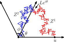
Figure 2: We split the Brownian path $Z$ in $\mathcal{C}_{\phi}$ from $u$ to $0$ at the time it first hits the ray $e^{i\theta}\mathbbm{R}_{+}$ for some $\theta\in(0,\phi)$ to get the subpaths $Z^{1}$ (red) and $Z^{2}$ (blue). We let $A$ be the duration of $Z^{1}$ and $L$ be such that $Le^{i\theta}$ is the endpoint of $Z^{1}$.

We now give a characterization of the inverse gamma distribution that implies Proposition 4.11.

Proposition 4.13.

Let $0<\theta<\phi<2\pi$ and $u>0$. Suppose $X$ is a real-valued random variable independent of $(A,L)$ as sampled in (4.15). Then

$$X\stackrel{{\scriptstyle d}}{{=}}A+\frac{L^{2}}{u^{2}}X$$ (4.16)

if and only if the law of $X$ is the inverse gamma distribution with shape $\frac{\pi}{\phi}$ and scale $\frac{u^{2}}{2}$ as described in Equation (2.2).

Proof of Proposition 4.11 given Proposition 4.13.

In (4.13), each of $\mathcal{A}_{0}$ and $\mathcal{A}_{1}$ agrees in law with the quantum area $X$ of a sample from $\mathcal{M}_{1,0}^{\mathrm{disk}}(\alpha;1)^{\#}$. Moreover, by Proposition 4.10 we have $\mathcal{A}_{1}$ independent of $(\mathcal{A},\mathcal{L})$, so by Lemma 4.12 we have $X\stackrel{{\scriptstyle d}}{{=}}A+\frac{L^{2}}{u^{2}}X$. Then Proposition 4.13 gives the law of $X$. Here the constraint $\alpha<Q-\frac{\gamma}{4}$ comes from $\phi=\frac{\gamma\pi}{2(Q-\alpha)}\in(0,2\pi)$. ∎

To prove Proposition 4.13, we need some basic properties about Brownian motion in cones whose full proofs we defer to Appendix A. See Figure 2 for an illustration.

Lemma 4.14.

Suppose $0<\theta<\phi<2\pi$ and $u>0$, and define $Z^{1},Z^{2}$ by the right hand side of (4.14). Let $A,L$ be defined as in (4.15), let $T$ be the sum of the durations of $Z^{1}$ and $Z^{2}$, and let $Y=\frac{u^{2}}{L^{2}}(T-A)$. Then both the laws of $T$ and $Y$ are the inverse gamma distribution with shape $\frac{\pi}{\phi}$ and scale $\frac{u^{2}}{2}$, and $Y$ is independent of $(A,L)$. Moreover, for $\varepsilon\in(0,\frac{\pi}{\phi})$, we have $\mathbbm{E}[(\frac{L}{u})^{\varepsilon}]<1$.

Proof.

By (4.14), the law of $T$ agrees with that of the duration of a sample from $\mathsf{m}_{\mathcal{C}_{\phi}}(u,0)^{\#}$, which by Corollary A.2 is the inverse gamma distribution with the desired parameters. By (4.14) and Brownian scaling, the conditional law of $Y$ given $(A,L)$ agrees with the law of the duration of a sample from $\mathsf{m}_{\mathcal{C}_{\phi}}(ue^{i\theta},0)^{\#}$, and so by Corollary A.2 it is the inverse gamma with shape $\frac{\pi}{\phi}$ and scale $\frac{u^{2}}{2}$. Finally, the claim $\mathbbm{E}[(\frac{L}{u})^{\varepsilon}]<1$ is Lemma A.5. ∎

Proof of Proposition 4.13.

With notation as in Lemma 4.14, we have $T=A+\frac{L^{2}}{u^{2}}Y$. Since each of $T,Y$ are distributed as inverse gamma with shape $\frac{\pi}{\phi}$ and scale $\frac{u^{2}}{2}$, and $Y$ is independent of $(A,L)$, we obtain the “if” direction of the proposition.

Now we check the converse. Let $(A_{1},L_{1}),\dots,(A_{n},L_{n})$ be independent copies of $(A,L)$ in (4.15). Suppose $X$ satisfies (4.16). For any positive integer $n$, iterating (4.16) $n$ times yields that $X$ has the same distribution as

$$A_{1}+\frac{L_{1}^{2}}{u^{2}}\mathopen{}\mathclose{{}\left(A_{2}+\frac{L_{2}^{2}}{u^{2}}\mathopen{}\mathclose{{}\left(\dots\mathopen{}\mathclose{{}\left(A_{n}+\frac{L_{n}^{2}}{u^{2}}X}\right)\dots}\right)}\right)=:S_{n}+\mathopen{}\mathclose{{}\left(\prod_{i=1}^{n}\frac{L_{i}^{2}}{u^{2}}}\right)X,$$

where $S_{n}$ is a function of $\{(A_{i},L_{i})\}_{1\leq i\leq n}$. Since Lemma 4.14 gives $\mathbbm{E}[\mathopen{}\mathclose{{}\left(\frac{L}{u}}\right)^{\varepsilon}]<1$ for some $\varepsilon>0$, by Markov’s inequality we have $\prod_{i=1}^{n}\frac{L_{i}^{2}}{u^{2}}\to 0$ in probability as $n\to\infty$, and hence $S_{n}\to X$ in distribution as $n\to\infty$. Thus any solution to (4.16) is the distributional limit of $S_{n}$, which is unique. ∎

4.4 From the inverse gamma distribution to the FZZ formula

Recall $\mathopen{}\mathclose{{}\left\langle e^{\alpha\phi(i)}}\right\rangle$ from Definition 2.5. By Definitions 2.5 and 4.2, for $\alpha\in(\frac{2}{\gamma},Q)$, $\mu\geq 0$ and $\mu_{B}>0$

$$\mathopen{}\mathclose{{}\left\langle e^{\alpha\phi(i)}}\right\rangle =\mathrm{LF}_{\mathbbm{H}}^{(\alpha,i)}[e^{-\mu\mu_{\phi}(\mathbbm{H})-\mu_{B}\nu_{\phi}(\mathbbm{R})}-1]$$

$$=\int_{0}^{\infty}\mathcal{M}_{1,0}^{\mathrm{disk}}(\alpha;\ell)[e^{-\mu A-\mu_{B}\ell}-1]\,d\ell$$

$$=\int_{0}^{\infty}|\mathcal{M}_{1,0}^{\mathrm{disk}}(\alpha;\ell)|\mathcal{M}_{1,0}^{\mathrm{disk}}(\alpha;\ell)^{\#}[e^{-\mu A-\mu_{B}\ell}-1]\,d\ell.$$

Here $A$ represents the quantum area of a quantum surface sampled from $\mathcal{M}_{1,0}^{\mathrm{disk}}(\alpha;\ell)$. Recall $\overline{U}_{0}(\alpha)$ from Proposition 2.8. By Lemma 4.4, we have

$$\mathopen{}\mathclose{{}\left\langle e^{\alpha\phi(i)}}\right\rangle=C\int_{0}^{\infty}\ell^{\frac{2}{\gamma}(\alpha-Q)-1}\mathcal{M}_{1,0}^{\mathrm{disk}}(\alpha;1)^{\#}[e^{-\mu\ell^{2}A-\mu_{B}\ell}-1]\,d\ell\quad\textrm{ for }\alpha\in(\frac{2}{\gamma},Q),$$ (4.17)

where $C=\frac{2}{\gamma}2^{-\frac{\alpha^{2}}{2}}\overline{U}_{0}(\alpha)$. By (4.17) and Proposition 4.11, we can prove Theorem 1.1 for $\alpha\in(\frac{2}{\gamma},Q-\frac{\gamma}{4})$.

Proposition 4.15.

$U(\alpha)=U_{\mathrm{FZZ}}(\alpha)$ for $\alpha\in(\frac{2}{\gamma},Q-\frac{\gamma}{4})$.

In order to prove Proposition 4.15, we first record two simple calculus facts which will allow us to relate the inverse gamma distribution to the FZZ formula.

Lemma 4.16.

Let $x\in(-1,1)$ and $a\in\mathbb{R}\setminus\mathbb{Z}$. The following expansion holds:

$$\cos(a\arccos x)=\frac{a}{2}\sin(\pi a)\sum_{n=0}^{+\infty}\frac{(-2)^{n-1}}{\pi n!}\Gamma(\frac{n+a}{2})\Gamma(\frac{n-a}{2})x^{n}.$$ (4.18)

Proof.

The function $T_{a}(x)=\cos(a\arccos x)$ is a generalization of Chebyshev polynomials, which reduces to the usual Chebyshev polynomials when $a$ is a positive integer. For $x\in(-1,1)$, Taylor expansion gives:

$$T_{a}(x) =a\sum_{n=0}^{+\infty}\frac{(2x)^{n}}{2(n!)}\cos(\frac{\pi}{2}(a-n))\frac{\Gamma(\frac{a+n}{2})}{\Gamma(\frac{a-n}{2}+1)}$$

$$=a\sum_{n=0}^{+\infty}\frac{(2x)^{n}}{2\pi n!}\cos(\frac{\pi}{2}(a-n))\Gamma(\frac{a+n}{2})\Gamma(-\frac{a-n}{2})\sin(\pi\frac{a-n}{2}+\pi)$$

$$=\frac{a}{2}\sin(\pi a)\sum_{n=0}^{+\infty}\frac{(-2)^{n-1}}{\pi n!}\Gamma(\frac{n+a}{2})\Gamma(\frac{n-a}{2})x^{n}.\qed$$

Lemma 4.17.

Let $a,b,c,\lambda\in\mathbb{R}$ satisfying $a>0$, $b>-1$, $c<\frac{b}{2}-\frac{1}{2}$, $0<\lambda<2a$. Then the following identity holds:

$$\int_{0}^{\infty}dy\;y^{b}e^{-\lambda y}\int_{0}^{\infty}dt\;t^{c}\exp\mathopen{}\mathclose{{}\left(-y^{2}t-\frac{a^{2}}{t}}\right)=\frac{1}{2}\sum_{n=0}^{+\infty}\frac{(-\lambda)^{n}}{n!}a^{-n+2c-b+1}\Gamma(\frac{n}{2}+\frac{b}{2}-c-\frac{1}{2})\Gamma(\frac{n}{2}+\frac{b}{2}+\frac{1}{2}).$$ (4.19)

Proof.

To compute the double integral we expand $e^{-\lambda y}$ and then perform the change of variable $u=y^{2}t$, $v=\frac{a^{2}}{t}$. Hence $y=\frac{\sqrt{uv}}{a}$, $t=\frac{a^{2}}{v}$, $dydt=\frac{a}{2v\sqrt{uv}}dudv$. Therefore:

$$\int_{0}^{\infty}dy\;y^{b}e^{-\lambda y}\int_{0}^{\infty}dt\;t^{c}\exp\mathopen{}\mathclose{{}\left(-y^{2}t-\frac{a^{2}}{t}}\right)$$

$$=\sum_{n=0}^{+\infty}\frac{(-\lambda)^{n}}{n!}\int_{0}^{\infty}dy\;y^{b+n}\int_{0}^{\infty}dt\;t^{c}\exp\mathopen{}\mathclose{{}\left(-y^{2}t-\frac{a^{2}}{t}}\right)$$

$$=\sum_{n=0}^{+\infty}\frac{(-\lambda)^{n}}{n!}\int_{0}^{\infty}\int_{0}^{\infty}dudv\frac{a}{2v\sqrt{uv}}a^{2c}v^{-c}a^{-b-n}(uv)^{\frac{b}{2}+\frac{n}{2}}e^{-u-v}$$

$$=\frac{1}{2}\sum_{n=0}^{+\infty}\frac{(-\lambda)^{n}}{n!}a^{-n+2c-b+1}\int_{0}^{\infty}\int_{0}^{\infty}dudv\;u^{\frac{b}{2}+\frac{n}{2}-\frac{1}{2}}v^{\frac{b}{2}+\frac{n}{2}-c-\frac{3}{2}}e^{-u-v}$$

$$=\frac{1}{2}\sum_{n=0}^{+\infty}\frac{(-\lambda)^{n}}{n!}a^{-n+2c-b+1}\Gamma(\frac{n}{2}+\frac{b}{2}-c-\frac{1}{2})\Gamma(\frac{n}{2}+\frac{b}{2}+\frac{1}{2}).$$

The conditions on the parameters are such to make the above integrals and series converge. For $n=0$ in the sum, the integrals over $u$ and $v$ converge respectively if $b>-1$ and $c<\frac{b}{2}-\frac{1}{2}$. The condition $\lambda>0$ is obvious. The condition $\lambda<2a$ is required for the series over $n$ to converge, as can be checked on the last line. ∎

Proof of Proposition 4.15.

To start off we assume that the parameters $\mu,\mu_{B}>0$ are chosen such that

$$\frac{\mu^{2}_{B}}{\mu}\sin\frac{\pi\gamma^{2}}{4}\in(0,1).$$ (4.20)

This constraint will then be lifted by an analyticity argument in the variable $\mu_{B}$. Applying integration by parts to the integration over $\ell$ in (4.17), we get

$$\mathopen{}\mathclose{{}\left\langle e^{\alpha\phi(i)}}\right\rangle =\frac{\gamma C}{2(\alpha-Q)}\int_{0}^{\infty}\ell^{\frac{2}{\gamma}(\alpha-Q)}\mathcal{M}_{1,0}^{\mathrm{disk}}(\alpha;1)^{\#}[(2\mu\ell A+\mu_{B})e^{-\mu\ell^{2}A-\mu_{B}\ell}]\,d\ell$$

$$=C^{\prime}\int_{0}^{\infty}y^{\frac{2}{\gamma}(\alpha-Q)}\mathcal{M}_{1,0}^{\mathrm{disk}}(\alpha;1)^{\#}\mathopen{}\mathclose{{}\left[(\lambda+2yA)e^{-\lambda y-y^{2}A}}\right]dy,$$ (4.21)

where $y=\sqrt{\mu}\ell$, $C^{\prime}=-\frac{\gamma C}{2(Q-\alpha)}\mu^{\frac{Q-\alpha}{\gamma}}$ and $\lambda=\frac{\mu_{B}}{\mu^{1/2}}$. Now we use Proposition 4.11 which requires to assume $\alpha<Q-\frac{\gamma}{4}$ and we apply twice Lemma 4.17 with $(a,b,c,\lambda)$ equal to

$$\mathopen{}\mathclose{{}\left(\frac{1}{2\sqrt{\sin\frac{\pi\gamma^{2}}{4}}},\frac{2}{\gamma}(\alpha-Q),\frac{2}{\gamma}(\alpha-Q)-1,\lambda}\right)\quad\text{and}\quad\mathopen{}\mathclose{{}\left(\frac{1}{2\sqrt{\sin\frac{\pi\gamma^{2}}{4}}},\frac{2}{\gamma}(\alpha-Q)+1,\frac{2}{\gamma}(\alpha-Q),\lambda}\right).$$

The constraints on $(a,b,c,\lambda)$ required by Lemma 4.17 are satisfied provided that $\alpha\in(\frac{2}{\gamma},Q)$ and that equation (4.20) holds. Hence one arrives at the following power series expansions in the parameter $\lambda$:

$$C^{\prime}\int_{0}^{\infty}y^{\frac{2}{\gamma}(\alpha-Q)}\mathcal{M}_{1}^{\mathrm{disk}}(\alpha;1)^{\#}\mathopen{}\mathclose{{}\left[\lambda e^{-\lambda y-y^{2}A}}\right]dy$$ (4.22)

$$\quad=-\frac{C^{\prime\prime}}{2}\sum_{n=0}^{\infty}\frac{(-\lambda)^{n+1}}{n!}\mathopen{}\mathclose{{}\left(2\sqrt{\sin\frac{\pi\gamma^{2}}{4}}}\right)^{n+\frac{2}{\gamma}(Q-\alpha)+1}\Gamma(\frac{n}{2}+\frac{1}{\gamma}(\alpha-Q)+\frac{1}{2})\Gamma(\frac{n}{2}+\frac{1}{\gamma}(Q-\alpha)+\frac{1}{2}),$$

and

$$C^{\prime}\int_{0}^{\infty}y^{\frac{2}{\gamma}(\alpha-Q)}\mathcal{M}_{1}^{\mathrm{disk}}(\alpha;1)^{\#}\mathopen{}\mathclose{{}\left[2yAe^{-\lambda y-y^{2}A}}\right]dy$$ (4.23)

$$\quad=C^{\prime\prime}\sum_{n=0}^{\infty}\frac{(-\lambda)^{n}}{n!}\mathopen{}\mathclose{{}\left(2\sqrt{\sin\frac{\pi\gamma^{2}}{4}}}\right)^{n+\frac{2}{\gamma}(Q-\alpha)}\Gamma(\frac{n}{2}+\frac{1}{\gamma}(\alpha-Q)+1)\Gamma(\frac{n}{2}+\frac{1}{\gamma}(Q-\alpha)),$$

where $C^{\prime\prime}=\frac{(4\sin\frac{\pi\gamma^{2}}{4})^{\frac{2}{\gamma}(\alpha-Q)}}{\Gamma(\frac{2}{\gamma}(Q-\alpha))}C^{\prime}$. By shifting the sum in (4.22) to start at $n=1$ and applying in (4.23) the following identity on the Gamma function

$$\Gamma(\frac{n}{2}+\frac{1}{\gamma}(\alpha-Q)+1)=\mathopen{}\mathclose{{}\left(\frac{n}{2}+\frac{1}{\gamma}(\alpha-Q)}\right)\Gamma(\frac{n}{2}+\frac{1}{\gamma}(\alpha-Q)),$$

we obtain

$$\mathopen{}\mathclose{{}\left\langle e^{\alpha\phi(i)}}\right\rangle =-\frac{C^{\prime\prime}}{2}\sum_{n=0}^{\infty}\frac{(-\lambda)^{n+1}}{n!}\mathopen{}\mathclose{{}\left(2\sqrt{\sin\frac{\pi\gamma^{2}}{4}}}\right)^{n+\frac{2}{\gamma}(Q-\alpha)+1}\Gamma(\frac{n}{2}+\frac{1}{\gamma}(Q-\alpha)+\frac{1}{2})\Gamma(\frac{n}{2}+\frac{1}{\gamma}(\alpha-Q)+\frac{1}{2})$$

$$+C^{\prime\prime}\sum_{n=0}^{\infty}\frac{(-\lambda)^{n}}{n!}\mathopen{}\mathclose{{}\left(2\sqrt{\sin\frac{\pi\gamma^{2}}{4}}}\right)^{n+\frac{2}{\gamma}(Q-\alpha)}\Gamma(\frac{n}{2}+\frac{1}{\gamma}(Q-\alpha))\Gamma(\frac{n}{2}+\frac{1}{\gamma}(\alpha-Q)+1)$$

$$=C^{\prime\prime}\frac{\alpha-Q}{\gamma}\sum_{n=0}^{\infty}\frac{(-\lambda)^{n}}{n!}\mathopen{}\mathclose{{}\left(2\sqrt{\sin\frac{\pi\gamma^{2}}{4}}}\right)^{n+\frac{2}{\gamma}(Q-\alpha)}\Gamma(\frac{n}{2}+\frac{1}{\gamma}(\alpha-Q))\Gamma(\frac{n}{2}+\frac{1}{\gamma}(Q-\alpha)),$$

To then obtain the claimed formula $U_{\mathrm{FZZ}}(\alpha)$, one simply needs to apply Lemma 4.16 with $a=\frac{2}{\gamma}(\alpha-Q)$ and $x=\lambda\sqrt{\sin\frac{\pi\gamma^{2}}{4}}$. Thanks again to (4.20) and the fact that $\alpha\in(\frac{2}{\gamma},Q)$, the conditions to apply the lemma are satisfied. This gives

$$\mathopen{}\mathclose{{}\left\langle e^{\alpha\phi(i)}}\right\rangle =2C^{\prime\prime}\frac{\alpha-Q}{\gamma}\frac{\pi\gamma}{(\alpha-Q)}\frac{1}{\sin(\frac{2\pi}{\gamma}(Q-\alpha))}\mathopen{}\mathclose{{}\left(2\sqrt{\sin\frac{\pi\gamma^{2}}{4}}}\right)^{\frac{2}{\gamma}(Q-\alpha)}\cos\mathopen{}\mathclose{{}\left(\frac{2}{\gamma}(\alpha-Q)\arccos\mathopen{}\mathclose{{}\left(\lambda\sqrt{\sin\frac{\pi\gamma^{2}}{4}}}\right)}\right)$$

$$=2C^{\prime\prime}\Gamma(\frac{2}{\gamma}(Q-\alpha))\Gamma(1-\frac{2}{\gamma}(Q-\alpha))\mathopen{}\mathclose{{}\left(2\sqrt{\sin\frac{\pi\gamma^{2}}{4}}}\right)^{\frac{2}{\gamma}(Q-\alpha)}\cos((\alpha-Q)\pi s),$$

where the definition of $s$ was given in (1.5); see also (4.24). We compute:

$$2C^{\prime\prime}\Gamma(\frac{2}{\gamma}(Q-\alpha))\Gamma(1-\frac{2}{\gamma}(Q-\alpha))\mathopen{}\mathclose{{}\left(2\sqrt{\sin\frac{\pi\gamma^{2}}{4}}}\right)^{\frac{2}{\gamma}(Q-\alpha)}$$

$$=\frac{4}{\gamma}(\sin\frac{\pi\gamma^{2}}{4})^{\frac{1}{\gamma}(\alpha-Q)}\mu^{\frac{Q-\alpha}{\gamma}}2^{-\frac{\alpha^{2}}{2}}\mathopen{}\mathclose{{}\left(2^{-\frac{\gamma}{2}\alpha}}\right)^{\frac{2}{\gamma}(Q-\alpha)}\mathopen{}\mathclose{{}\left(\frac{\pi}{\Gamma(1-\frac{\gamma^{2}}{4})}}\right)^{\frac{2}{\gamma}(Q-\alpha)}\Gamma(\frac{\gamma}{2}(\alpha-\frac{\gamma}{2}))\Gamma(\frac{2\alpha}{\gamma}-\frac{4}{\gamma^{2}}-1)$$

$$=\frac{4}{\gamma}2^{-\frac{\alpha^{2}}{2}}\mathopen{}\mathclose{{}\left(\frac{\pi\mu}{2^{\gamma\alpha}}\frac{\Gamma(\frac{\gamma^{2}}{4})}{\Gamma(1-\frac{\gamma^{2}}{4})}}\right)^{\frac{Q-\alpha}{\gamma}}\Gamma(\frac{\gamma\alpha}{2}-\frac{\gamma^{2}}{4})\Gamma(\frac{2\alpha}{\gamma}-\frac{4}{\gamma^{2}}-1)=U_{\mathrm{FZZ}}(\alpha)/\cos((\alpha-Q)\pi s).$$

Putting everything together we conclude that $\mathopen{}\mathclose{{}\left\langle e^{\alpha\phi(i)}}\right\rangle=U(\alpha)=U_{\mathrm{FZZ}}(\alpha)$ provided that the condition (4.20) holds.

We will now extend the result by analyticity in $\mu_{B}$ to the full range of $\mu_{B}\in(0,+\infty)$. Notice $U_{\mathrm{FZZ}}(\alpha)$ contains the factor $\cos((\alpha-Q)\pi s)$ where $s$ and $\mu_{B}$ are related by:

$$\mu_{B}=\mu_{B}(s)=\sqrt{\frac{\mu}{\sin\frac{\pi\gamma^{2}}{4}}}\cos\frac{\pi\gamma s}{2}.$$ (4.24)

We want to find an open domain $D\subset\mathbb{C}$ of $s$ where the map $s\mapsto\mu_{B}(s)$ will be biholomorphic onto its image. Since $\frac{d}{ds}_{|s=0}\cos\frac{\pi\gamma s}{2}=0$, we cannot include $0$ in $D$. Since $\cos\frac{\pi\gamma s}{2}=1-\frac{\pi^{2}\gamma^{2}}{8}s^{2}+o(s^{2})$ and the second order $s^{2}$ is non-zero, we can include the sector $S_{\epsilon,\delta}:=\{re^{i\theta}|\theta\in(-\epsilon,\frac{\pi}{2}+\epsilon),0<r<\delta\}$ for two small parameters $\epsilon,\delta>0$. Indeed in $S_{\epsilon,\delta}$ the angle $\theta$ is contained in an interval of length strictly less than $\pi$. We also want $D$ to contain an open neighborhood in $\mathbb{C}$ of $i(\frac{\delta}{2},+\infty)$ where we wish to extend the equality $U(\alpha)=U_{\mathrm{FZZ}}(\alpha)$ and an open neighborhood of $(\frac{\delta}{2},\frac{1}{2\gamma})$ were we have already established it. From all these considerations we choose:

$$D:=S_{\epsilon,\delta}\cup\mathopen{}\mathclose{{}\left\{x+iy|x\in(\frac{\delta}{2},\frac{1}{2\gamma}),y\in(-\frac{\delta}{4},\frac{\delta}{4})}\right\}\cup\mathopen{}\mathclose{{}\left\{x+iy|x\in(-\frac{\delta}{4},\frac{\delta}{4}),y\in(\frac{\delta}{2},+\infty)}\right\}.$$

For $\epsilon,\delta$ small, the map $s\mapsto\mu_{B}(s)$ is then a biholomorphic map from $D$ onto its image, an open domain we call $D^{\prime}$. Now the exact formula $U_{\mathrm{FZZ}}(\alpha)$ is clearly an analytic function of $\mu_{B}$ on $D^{\prime}$. We must argue the same is true for the probabilistic definition $U(\alpha)=\mathopen{}\mathclose{{}\left\langle e^{\alpha\phi(i)}}\right\rangle$. For all $\mu_{B}\in D^{\prime}$, one clearly has $\operatorname{Re}(\mu_{B})>0$ which by Lemma 2.6 gives finiteness of $\mathopen{}\mathclose{{}\left|\mathopen{}\mathclose{{}\left\langle e^{\alpha\phi(i)}}\right\rangle}\right|$. Moreover, $\mathrm{LF}_{\mathbbm{H}}^{(\alpha,i)}\mathopen{}\mathclose{{}\left[\mathopen{}\mathclose{{}\left|\nu_{\phi}(\mathbbm{R})e^{-\mu\mu_{\phi}(\mathbbm{H})-\mu_{B}\nu_{\phi}(\mathbbm{R})}}\right|}\right]$ is also finite in the same region. This implies that $\mathrm{LF}_{\mathbbm{H}}^{(\alpha,i)}[-\mu_{B}\nu_{\phi}(\mathbbm{R})e^{-\mu\mu_{\phi}(\mathbbm{H})-\mu_{B}\nu_{\phi}(\mathbbm{R})}]$ is analytic in $\mu_{B}$ when $\operatorname{Re}(\mu_{B})>0$. Taking anti-derivative in $\mu_{B}$ and use Fubini theorem to interchange the integral in $\mu_{B}$ and $\mathrm{LF}_{\mathbbm{H}}^{(\alpha,i)}$, we see that $\mathopen{}\mathclose{{}\left\langle e^{\alpha\phi(i)}}\right\rangle=\mathrm{LF}_{\mathbbm{H}}^{(\alpha,i)}[e^{-\mu\mu_{\phi}(\mathbbm{H})-\mu_{B}\nu_{\phi}(\mathbbm{R})}-1]$ is analytic in $\mu_{B}$ when $\operatorname{Re}(\mu_{B})>0$. Since the equality of analytic functions $U(\alpha)=U_{\mathrm{FZZ}}(\alpha)$ in the variable $\mu_{B}$ holds on the interval given by (4.20) which is contained in the open set $D^{\prime}$, it holds on all of $D^{\prime}$. In particular it holds for $\frac{\mu_{B}}{\sqrt{\mu}}\sqrt{\sin\frac{\pi\gamma^{2}}{4}}\in(1,+\infty)$. By continuity we recover the equality at the special value $\frac{\mu_{B}}{\sqrt{\mu}}\sqrt{\sin\frac{\pi\gamma^{2}}{4}}=1$. This completes the proof. ∎

4.5 Analyticity in $\alpha$ and the proof of Theorem 1.1

In this section we prove that $U(\alpha)$ is complex analytic in $\alpha$ around $(\frac{2}{\gamma},Q)$. The proof utilizes the method given first in [KRV20] and in [RZ22], adapted to the case where there are both area and boundary GMC measures in the correlation function. Together with Proposition 4.15 this will conclude the proof of Theorem 1.1. We will then prove Corollary 4.19 and Theorem 1.2 that extend the range of $\alpha$ from $(\frac{2}{\gamma},Q)$ to $(\frac{\gamma}{2},Q)$.

Proposition 4.18.

For any compact set $K\subset(\frac{2}{\gamma},Q)$, the function $\alpha\rightarrow U(\alpha)$ is complex analytic on a complex neighborhood of the set $K$.

Proof.

To start we use the following identity coming from Lemma 2.6

$$\mathopen{}\mathclose{{}\left\langle e^{\alpha\phi(2i)}}\right\rangle=\frac{U(\alpha)}{\mathopen{}\mathclose{{}\left|\operatorname{Im}2i}\right|^{2\Delta_{\alpha}}},$$ (4.25)

to place the bulk insertion at the location $2i$, and will prove that $\mathopen{}\mathclose{{}\left\langle e^{\alpha\phi(2i)}}\right\rangle$ is analytic in $\alpha$. Fix a $r_{0}$ such that $e^{-r_{0}}<\frac{1}{2}$. Let $h$ be the free boundary GFF on $\mathbb{H}$, which is normalized to have zero average over the upper half unit circle. Thanks to the Markov property of the field, see for instance [BP, Theorem 5.5], we can write the decomposition $h=h_{1}+h_{2}$, where $h_{1}$ is a Dirichlet GFF on $B(2i,e^{-r_{0}})$ and $h_{2}$ is a field which is independent of $h_{1}$ and smooth in a neighborhood of $2i$. Notice we placed the insertion at $2i$ so $B(2i,e^{-r_{0}})$ does not intersect the upper half unit circle. Consider now the one-dimensional process $h_{1,r}(2i)$ obtained by taking the mean of $h_{1}(2i)$ over the circles of radius $e^{-r}$ centered at $2i$, assuming $r\geq r_{0}$. The main fact we will use about this field is that $h_{1,r+t}(2i)-h_{1,r}(2i)$ is a Brownian motion independent of $(h(z))_{z\in\mathbb{H}_{r}}$, where $\mathbb{H}_{r}:=\mathbb{H}\backslash B(2i,e^{-r})$. Record also that $\mathbbm{E}[h_{1,r}(2i)^{2}]=r-r_{0}$ and the notation $h_{r}:=h_{1,r}+h_{2}$. From these facts we can deduce that:

$$\mathbb{E}\mathopen{}\mathclose{{}\left[e^{\alpha h_{1,r+1}(2i)-\frac{\alpha^{2}}{2}\mathbb{E}[h_{1,r+1}(2i)^{2}]}F\mathopen{}\mathclose{{}\left((h(z))_{z\in\mathbb{H}_{r}}}\right)}\right]$$

$$=e^{\frac{\alpha^{2}}{2}\mathbb{E}[h_{1,r}(2i)^{2}]-\frac{\alpha^{2}}{2}\mathbb{E}[h_{1,r+1}(2i)^{2}]}\mathbb{E}\mathopen{}\mathclose{{}\left[e^{\alpha h_{1,r+1}(2i)-\alpha h_{1,r}(2i)}}\right]\mathbb{E}\mathopen{}\mathclose{{}\left[e^{\alpha h_{1,r}(2i)-\frac{\alpha^{2}}{2}\mathbb{E}[h_{1,r}(2i)^{2}]}F\mathopen{}\mathclose{{}\left((h(z))_{z\in\mathbb{H}_{r}}}\right)}\right]$$

$$=\mathbb{E}\mathopen{}\mathclose{{}\left[e^{\alpha h_{1,r}(2i)-\frac{\alpha^{2}}{2}\mathbb{E}[h_{1,r}(2i)^{2}]}F\mathopen{}\mathclose{{}\left((h(z))_{z\in\mathbb{H}_{r}}}\right)}\right]$$

$$\Rightarrow\> \mathbb{E}\mathopen{}\mathclose{{}\left[e^{\alpha h_{r}(2i)-\frac{\alpha^{2}}{2}\mathbb{E}[h_{r}(2i)^{2}]}F\mathopen{}\mathclose{{}\left((h(z))_{z\in\mathbb{H}_{r}}}\right)}\right]=\mathbb{E}\mathopen{}\mathclose{{}\left[e^{\alpha h_{r+1}(2i)-\frac{\alpha^{2}}{2}\mathbb{E}[h_{r+1}(2i)^{2}]}F\mathopen{}\mathclose{{}\left((h(z))_{z\in\mathbb{H}_{r}}}\right)}\right].$$

Now we can obtain $U(\alpha)$ from the following limit $U(\alpha)=2^{-\frac{\alpha^{2}}{2}}\lim_{r\to\infty}U_{r}(\alpha)$, where we have introduced:

$$U_{r}(\alpha)=\int_{\mathbb{R}}dce^{(\alpha-Q)c}\mathbb{E}\mathopen{}\mathclose{{}\left[e^{\alpha h_{r}(2i)-\frac{\alpha^{2}}{2}\mathbb{E}[h_{r}(2i)^{2}]}\mathopen{}\mathclose{{}\left(\exp\mathopen{}\mathclose{{}\left(-e^{\gamma c}\mu_{h}(\mathbb{H}_{r})-e^{\frac{\gamma}{2}c}\nu_{h}(\mathbb{R})}\right)-1}\right)}\right].$$

When $\alpha$ is a complex number, we write $\alpha=a+ib$. We want to prove there exists a complex neighborhood $V$ containing the set $K$ such that for any compact set $K^{\prime}$ contained in $V$, $U_{r}(\alpha)$ converges uniformly as $r\rightarrow+\infty$ over $K^{\prime}$. Setting $\tilde{h}(z):=h(z)+aG_{\mathbb{H}}(z,2i)$, we have the following:

$$|U_{r+1}(\alpha)-U_{r}(\alpha)|$$

$$=\int_{\mathbb{R}}dc\mathopen{}\mathclose{{}\left|e^{(\alpha-Q)c}\mathbb{E}\mathopen{}\mathclose{{}\left[e^{\alpha h_{r+1}(2i)-\frac{\alpha^{2}}{2}\mathbb{E}[h_{r+1}(2i)^{2}]}\exp\mathopen{}\mathclose{{}\left(-e^{\frac{\gamma}{2}c}\nu_{h}(\mathbb{R})}\right)\mathopen{}\mathclose{{}\left(\exp\mathopen{}\mathclose{{}\left(-e^{\gamma c}\mu_{h}(\mathbb{H}_{r+1})}\right)-\exp\mathopen{}\mathclose{{}\left(-e^{\gamma c}\mu_{h}(\mathbb{H}_{r})}\right)}\right)}\right]}\right|$$

$$\leq C\,e^{\frac{r+1}{2}b^{2}}\int_{\mathbb{R}}dce^{(a-Q)c}\mathbb{E}\mathopen{}\mathclose{{}\left[\exp\mathopen{}\mathclose{{}\left(-e^{\frac{\gamma}{2}c}\nu_{\tilde{h}}(\mathbb{R})}\right)\mathopen{}\mathclose{{}\left|\exp\mathopen{}\mathclose{{}\left(-e^{\gamma c}\mu_{\tilde{h}}(\mathbb{H}_{r+1})}\right)-\exp\mathopen{}\mathclose{{}\left(-e^{\gamma c}\mu_{\tilde{h}}(\mathbb{H}_{r})}\right)}\right|}\right]$$

$$\leq C\,e^{\frac{r+1}{2}b^{2}}\int_{\mathbb{R}}dce^{(a-Q)c}\mathbb{E}\mathopen{}\mathclose{{}\left[\exp\mathopen{}\mathclose{{}\left(-e^{\gamma c}\mu_{\tilde{h}}(\mathbb{H}_{r+1})}\right)-\exp\mathopen{}\mathclose{{}\left(-e^{\gamma c}\mu_{\tilde{h}}(\mathbb{H}_{r})}\right)}\right]$$

$$=C^{\prime}e^{\frac{r+1}{2}b^{2}}\mathbbm{E}\mathopen{}\mathclose{{}\left[\mu_{\widetilde{h}}(\mathbb{H}_{r+1})^{\frac{Q-a}{\gamma}}-\mu_{\widetilde{h}}(\mathbb{H}_{r})^{\frac{Q-a}{\gamma}}}\right].$$

From the second line to the third, we have applied the Girsanov theorem to the real part of $\alpha h_{r+1}(2i)$, before moving the absolute value inside the expression. The last equality follows from changing the integration variable from $c$ to $y=e^{\gamma c}\mu_{\widetilde{h}}(\mathbbm{H}_{i})$ for $i=r,r+1$. Thus,

$$|U_{r+1}(\alpha)-U_{r}(\alpha)|\leq C^{\prime}e^{\frac{r+1}{2}b^{2}}\mathbbm{E}\mathopen{}\mathclose{{}\left[\mu_{\widetilde{h}}(\mathbbm{H}_{r+1}\backslash\mathbbm{H}_{r})^{\frac{Q-a}{\gamma}}}\right]\leq C^{\prime\prime}e^{\frac{r+1}{2}b^{2}}e^{ra(Q-a)}\mathbbm{E}\mathopen{}\mathclose{{}\left[\mu_{h}(\mathbbm{H}_{r+1}\backslash\mathbbm{H}_{r})^{\frac{Q-a}{\gamma}}}\right].$$

The first inequality follows from $(a+b)^{s}\leq a^{s}+b^{s}$ for $s\in(0,1)$, and the second since $\widetilde{h}$ and $h$ differ by roughly $ar$ on $\mathbbm{H}_{r+1}\backslash\mathbbm{H}_{r}$.

By the multifractal scaling of GMC, see e.g. [BP, Section 3.6] or [RV14, Section 4], we have

$$\mathbbm{E}[\mu_{h}(\mathbbm{H}_{r+1}\backslash\mathbbm{H}_{r})^{\frac{Q-a}{\gamma}}]\asymp e^{(-\gamma Qq+\frac{\gamma^{2}q^{2}}{2})r},\qquad q=\frac{Q-a}{\gamma}.$$

Combining with the previous inequality, we deduce that $|U_{r+1}(\alpha)-U_{r}(\alpha)|\lesssim e^{r(\frac{b^{2}}{2}-\frac{1}{2}(Q-a)^{2})}$. Choosing the open set $V$ in such a way that $\frac{b^{2}}{2}<\frac{1}{2}(Q-a)^{2}$ always holds, all the inequalities we have done before hold true and hence we have shown that $U_{r}(\alpha)$ converges locally uniformly. Since $U_{r}(\alpha)$ is complex analytic in $\alpha$, this proves the analyticity result of $U(\alpha)$. ∎

Proof of Theorem 1.1 .

From the exact formula, $U_{\mathrm{FZZ}}(\alpha)$ is a meromorphic function of $\alpha$ on $\mathbbm{C}$. By uniqueness of the meromorphic continuation, Propositions 4.15 and 4.18, we have $U(\alpha)=U_{\mathrm{FZZ}}(\alpha)$ for all $\alpha\in(\frac{2}{\gamma},Q)$. ∎

Proof of Theorem 1.2.

Proposition 4.11 proves the theorem for $\alpha\in(\frac{\gamma}{2},Q-\frac{\gamma}{4})$. To complete the proof we consider $\alpha\in[Q-\frac{\gamma}{4},Q)$. Let $L$ be sampled from the power law $\frac{2}{\gamma}2^{-\frac{\alpha^{2}}{2}}\overline{U}_{0}(\alpha)\ell^{\frac{2}{\gamma}(\alpha-Q)-1}\,d\ell$ where $\overline{U}_{0}$ is as in Lemma 2.7, and let $A=L^{2}X$ where $X$ is sampled from an independent inverse gamma distribution with shape $\frac{2}{\gamma}(Q-\alpha)$ and scale $\frac{1}{4\sin\frac{\pi\gamma^{2}}{4}}$. Let $\Pi$ be the joint law of $(A,L)$. Proposition 4.15 proves that $\Pi[e^{-\mu A-\mu_{B}L}-1]=U_{\mathrm{FZZ}}(\alpha)$ for $\alpha\in(\frac{2}{\gamma},Q-\frac{\gamma}{4})$, but the argument works equally well for our range $\alpha\in[Q-\frac{\gamma}{4},Q)$. Thus $\mathrm{LF}_{\mathbbm{H}}^{(\alpha,i)}[e^{-\mu\mu_{\phi}(\mathbbm{H})-\mu_{B}\nu_{\phi}(\mathbbm{R})}-1]=\Pi[e^{-\mu A-\mu_{B}L}-1]$ by Theorem 1.1, so $\mathrm{LF}_{\mathbbm{H}}^{(\alpha,i)}[\nu_{\phi}(\mathbbm{R})e^{-\mu\mu_{\phi}(\mathbbm{H})-\mu_{B}\nu_{\phi}(\mathbbm{R})}]=\Pi[Le^{-\mu A-\mu_{B}L}]$. Therefore by standard arguments of characterization of a law by the Laplace transform, the joint law of $(\mu_{\phi}(\mathbbm{H}),\nu_{\phi}(\mathbbm{R}))$ under $\mathrm{LF}_{\mathbbm{H}}^{(\alpha,i)}$ is the same as that of $(A,L)$ under $\Pi$, which concludes the proof. ∎

Since we have now established Theorem 1.2 for the whole range $\alpha\in(\frac{\gamma}{2},Q)$, we have the following extension of the probabilistic definition of $U(\alpha)$ and of Theorem 1.1, for which we omit the proof.

Corollary 4.19.

Let $\alpha\in(\frac{\gamma}{2},Q)$. For $k\in\mathbb{N}$ and $\alpha\in(Q-\frac{\gamma(k+1)}{2},Q-\frac{\gamma k}{2})$, we define $U(\alpha)$ by:

$$U(\alpha)=\frac{2}{\gamma}2^{-\frac{\alpha^{2}}{2}}\overline{U}_{0}(\alpha)\int_{0}^{\infty}\ell^{\frac{2}{\gamma}(\alpha-Q)-1}\mathbbm{E}\mathopen{}\mathclose{{}\left[e^{-\mu\ell^{2}A-\mu_{B}\ell}-\sum_{i=0}^{k}c_{i}(A)\ell^{i}}\right]\,d\ell.$$ (4.26)

Here the expectation is with respect to the law of $A$ which is distributed according to the inverse gamma distribution with shape $\frac{2}{\gamma}(Q-\alpha)$ and scale $\frac{1}{4\sin^{2}\frac{\pi\gamma^{2}}{4}}$. $\overline{U}_{0}(\alpha)$ is given by the explicit formula (2.6). Lastly the constants $c_{i}(A)$ are specified by the following expansion in powers of $\ell$:

$$e^{-\mu\ell^{2}A-\mu_{B}\ell}=\sum_{i=0}^{k}c_{i}(A)\ell^{i}+O(\ell^{i+1}).$$ (4.27)

Then this definition of $U(\alpha)$ is the meromorphic extension of (1.8) on $(Q-\frac{\gamma(k+1)}{2},Q-\frac{\gamma k}{2})$ and it obeys $U(\alpha)=U_{\mathrm{FZZ}}(\alpha)$.

Finally, we provide a commonly used form of the FZZ formula; see [FZZ00, (2.44)].

Proposition 4.20.

For $\alpha\in(\frac{\gamma}{2},Q)$ and $\ell>0$, writing $A$ for the random area of a sample from $\mathcal{M}_{1}^{\mathrm{disk}}(\alpha;\ell)$, we have

$$\mathcal{M}_{1}^{\mathrm{disk}}(\alpha;\ell)[e^{-\mu A}]=\frac{2}{\gamma}2^{-\frac{\alpha^{2}}{2}}\overline{U}_{0}(\alpha)\ell^{-1}\frac{2}{\Gamma(\frac{2}{\gamma}(Q-\alpha))}\mathopen{}\mathclose{{}\left(\frac{1}{2}\sqrt{\frac{\mu}{\sin(\pi\gamma^{2}/4)}}}\right)^{\frac{2}{\gamma}(Q-\alpha)}K_{\frac{2}{\gamma}(Q-\alpha)}\mathopen{}\mathclose{{}\left(\ell\sqrt{\frac{\mu}{\sin(\pi\gamma^{2}/4)}}}\right).$$

Here, $K_{\nu}(x)$ is the modified Bessel function of the second kind; see e.g. [DLMF, Section 10.25].

Proof.

By Theorem 1.2, writing $\beta=\frac{1}{4\sin\frac{\pi\gamma^{2}}{4}}$ and considering $\ell=1$, we have

$$\mathcal{M}_{1}^{\mathrm{disk}}(\alpha;1)^{\#}[e^{-\mu A}] =\frac{\beta^{\frac{2}{\gamma}(Q-\alpha)}}{\Gamma(\frac{2}{\gamma}(Q-\alpha))}\int_{0}^{\infty}t^{-\frac{2}{\gamma}(Q-\alpha)-1}\exp^{-\frac{\beta}{t}-\mu t}\,dt$$

$$=\frac{2}{\Gamma(\frac{2}{\gamma}(Q-\alpha))}(\mu\beta)^{\frac{1}{\gamma}(Q-\alpha)}K_{\frac{2}{\gamma}(Q-\alpha)}(\sqrt{4\mu\beta}),$$

where the last equality follows from a change of variables $s=\mu t$ and the integral identity $K_{\nu}(z)=\frac{1}{2}(\frac{1}{2}z)^{\nu}\int_{0}^{\infty}\exp(-s-\frac{z^{2}}{4s})\frac{ds}{s^{\nu+1}}$ [DLMF, Eq. 10.32.10] with the choice $z=\sqrt{4\mu\beta}$ and $\nu=\frac{2}{\gamma}(Q-\alpha)$. Since for general $\ell$ we have $\mathcal{M}_{1}^{\mathrm{disk}}(\alpha;\ell)^{\#}[e^{-\mu A}]=\mathcal{M}_{1}^{\mathrm{disk}}(\alpha;1)^{\#}[e^{-\mu\ell^{2}A}]$,

$$\mathcal{M}_{1}^{\mathrm{disk}}(\alpha;\ell)^{\#}[e^{-\mu A}]=\frac{2}{\Gamma(\frac{2}{\gamma}(Q-\alpha))}\ell^{\frac{2}{\gamma}(Q-\alpha)}\mathopen{}\mathclose{{}\left(\frac{1}{2}\sqrt{\frac{\mu}{\sin(\pi\gamma^{2}/4)}}}\right)^{\frac{2}{\gamma}(Q-\alpha)}K_{\frac{2}{\gamma}(Q-\alpha)}\mathopen{}\mathclose{{}\left(\ell\sqrt{\frac{\mu}{\sin(\pi\gamma^{2}/4)}}}\right).$$

By Lemma 2.7 we have $|\mathcal{M}_{1}^{\mathrm{disk}}(\alpha;\ell)|=\frac{2}{\gamma}2^{-\frac{\alpha^{2}}{2}}\overline{U}_{0}(\alpha)\ell^{\frac{2}{\gamma}(\alpha-Q)-1}$, so the result follows. ∎

5 Proof of the SLE bubble zipper with a $\gamma$-bulk insertion

In this section we prove Theorem 4.1. For technical convenience, we will consider loops on $\mathbbm{H}$ passing through $\infty$ instead of $0$. More precisely, let $\psi(z)=-z^{-1}$ and $\mathrm{Bubble}_{\mathbbm{H}}(i,\infty)=\{\eta:\psi(\eta)\in\mathrm{Bubble}_{\mathbbm{H}}(i,0)\}$. We will find a measure on $\mathrm{Bubble}_{\mathbbm{H}}(i,\infty)$ with the desired property and then use $\psi$ to pull it back to get $\mathsf{m}$ in Theorem 4.1. The proof is a limiting argument based on Lemma 3.15 and a three-disk variant of the conformal welding result in Theorem 2.13. We set up the framework of the proof in Section 5.1 and carry out the details in Sections 5.2 and 5.3.

5.1 A conformal welding of three quantum disks

Set $\kappa=\gamma^{2}$. Let $\eta_{1}$ be an $\operatorname{SLE}_{\kappa}(\frac{\gamma^{2}}{2}-2,\frac{\gamma^{2}}{2})$ curve on $(\mathbbm{H},0,\infty)$. Let $H^{+}_{\eta_{1}}$ the be right component of $\mathbbm{H}\setminus\eta_{1}$. Conditioning on $\eta_{1}$, let $\eta_{2}$ be an $\operatorname{SLE}_{\kappa}(0;\frac{\gamma^{2}}{2}-2)$ on $(\mathbbm{H}_{\eta_{1}}^{+},0,\infty)$. We denote $\mathcal{P}(\mathbbm{H},0,\infty)$ as the law of $(\eta_{1},\eta_{2})$. For a general simply connected domain $D$ with two boundary points $(a,b)$, we write $\mathcal{P}(D,a,b)$ as the conformal image of $\mathcal{P}(\mathbbm{H},0,\infty)$. As a straightforward extension of Theorem 2.13, we have the following conformal welding result.

Theorem 5.1.

Let $\ell,\ell^{\prime}>0$ and $(\mathbbm{H},\phi,0,\infty)$ be an embedding of a sample from $\mathcal{M}^{\mathrm{disk}}_{0,2}(2+\gamma^{2};\ell,\ell^{\prime})$. Let $(\eta_{1},\eta_{2})$ be sampled from $\mathcal{P}(\mathbbm{H},0,\infty)$ independent of $\phi$. Let $\mathbbm{H}^{1}_{\eta}$, $\mathbbm{H}^{12}_{\eta}$ and $\mathbbm{H}^{2}_{\eta}$ be the left, middle, and right components of $\mathbbm{H}\setminus(\eta_{1}\cup\eta_{2})$, respectively. The joint law of $(\mathbbm{H}^{1}_{\eta},\phi,0,\infty)$, $(\mathbbm{H}^{12}_{\eta},\phi,0,\infty)$, and $(\mathbbm{H}^{2}_{\eta},\phi,0,\infty)$ viewed as marked quantum surfaces equals

$$C\iint_{0}^{\infty}\mathcal{M}_{0,2}^{\mathrm{disk}}(\frac{\gamma^{2}}{2};\ell;p)\times\mathcal{M}_{0,2}^{\mathrm{disk}}(2;p;q)\times\mathcal{M}_{0,2}^{\mathrm{disk}}(\frac{\gamma^{2}}{2};q;\ell^{\prime})\,dp\,dq,\quad\textrm{ for some }C\in(0,\infty).$$ (5.1)

Proof.

This is [AHS20, Theorem 2.3] when $W_{1}=W_{3}=\frac{\gamma^{2}}{2}$ and $W_{2}=2$. ∎

Fix $\delta\in(0,\frac{1}{2})$. Sample $(\phi,\mathbf{x})$ from $\mathrm{LF}_{\mathbbm{H}}^{(\gamma,i)}\times dx$ and sample $(\eta_{1},\eta_{2})$ from $\mathcal{P}(\mathbbm{H},\mathbf{x},\infty)$, and restrict to the event that $\nu_{\phi}(\mathbf{x},\infty)\in(\delta,\frac{1}{2})$, $\nu_{\phi}(\mathbbm{R})\in(1,2)$ and $i$ is in between $\eta_{1}$ and $\eta_{2}$. Here and later, we write $\nu_{\phi}(a,b)$ to denote the $\nu_{\phi}$-length of the interval $(a,b)$. Let $M_{\delta}$ be the law of $(\phi,\mathbf{x},\eta_{1},\eta_{2})$ (restricted to the aforementioned event). See Figure 3.

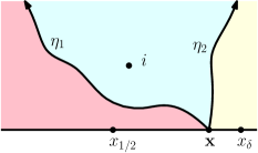
Figure 3: Illustration of $(\phi,\mathbf{x},\eta_{1},\eta_{2})$ under $M_{\delta}$. Sample $(\phi,\mathbf{x})$ from $\mathrm{LF}_{\mathbbm{H}}^{(\gamma,i)}\times dx$ and sample $(\eta_{1},\eta_{2})$ from $\mathcal{P}(\mathbbm{H},\mathbf{x},\infty)$. To represent geometrically the condition $\nu_{\phi}(\mathbf{x},\infty)\in(\delta,\frac{1}{2})$, consider the points $x_{1/2}$ and $x_{\delta}$ such that $\nu_{\phi}(x_{1/2},\infty)=1/2$ and $\nu_{\phi}(x_{\delta},\infty)=\delta$. Then $M_{\delta}$ is obtained by restricting to the event $\mathbf{x}\in(x_{1/2},x_{\delta})$, $i$ is in the middle of $\eta_{1}$ and $\eta_{2}$ and $\nu_{\phi}(\mathbbm{R})\in(1,2)$. Lemma 5.2 describes the law of the three shaded quantum surfaces.

Lemma 5.2.

There exists $C>0$ such that for each $\delta\in(0,\frac{1}{2})$, if $(\phi,\mathbf{x},\eta_{1},\eta_{2})$ is sampled from $M_{\delta}$ then the law of the three marked quantum surfaces of $(\mathbbm{H},\phi,\eta_{1},\eta_{2},i,\mathbf{x},\infty)$ bounded by $\eta_{1}$, $\eta_{2}$ and $\partial\mathbbm{H}$ is given by

$$C\int_{\delta}^{1/2}\int_{1-b}^{2-b}\int_{0}^{\infty}\int_{0}^{\infty}\mathcal{M}_{0,2}^{\mathrm{disk}}(\frac{\gamma^{2}}{2};a,p)\times\mathcal{M}^{\mathrm{disk}}_{1,2}(2;p,q)\times\mathcal{M}_{0,2}^{\mathrm{disk}}(\frac{\gamma^{2}}{2};q,b)\,dq\,dp\,da\,db.$$ (5.2)

Proof.

Lemma 3.15 states that if we sample $(\phi,\mathbf{x})$ from $\mathrm{LF}_{\mathbbm{H}}^{(\gamma,i)}\times dx$ then the law of the quantum surface $(\mathbbm{H},\phi,i,\mathbf{x},\infty)$ is $C\mathcal{M}_{1,2}^{\mathrm{disk}}(2+\gamma^{2})$ for some constant $C$. If we further sample $(\eta_{1},\eta_{2})$ from $\mathcal{P}(\mathbbm{H},\mathbf{x},\infty)$ and restrict to the event that $i$ lies between $\eta_{1}$ and $\eta_{2}$, then by Definition 3.10 and Theorem 5.1, the quantum surface $(\mathbbm{H},\phi,\eta_{1},\eta_{2},i,\mathbf{x},\infty)$ has law

$$C\iiiint_{0}^{\infty}\mathcal{M}_{0,2}^{\mathrm{disk}}(\frac{\gamma^{2}}{2};a,p)\times\mathcal{M}^{\mathrm{disk}}_{1,2}(2;p,q)\times\mathcal{M}_{0,2}^{\mathrm{disk}}(\frac{\gamma^{2}}{2};q,b)\,dq\,dp\,da\,db$$

for some $C>0$. Further restricting to the event $\nu_{\phi}(\mathbf{x},\infty)\in(\delta,\frac{1}{2})$ and $\nu_{\phi}(\mathbbm{R})\in(1,2)$ we conclude the proof. ∎

In Section 5.2, we will show that the probability measure $M^{\#}_{\delta}$ that is proportional to $M_{\delta}$ concentrates on the event that $\nu_{h}(\mathbf{x},\infty)$ is of order $\delta$ and $\log\mathbf{x}$ is of order $\log\delta^{-1}$. This effectively collapses the right boundary of $(\mathbbm{H},\phi,\mathbf{x},\infty)$. Building on this, we will prove the following proposition. Recall that for two probability measures $P,Q$ on the same measure space, the total variation distance between $P$ and $Q$ is $\sup_{A}|P(A)-Q(A)|$ where the supremum is taken over all measurable sets.

Proposition 5.3.

For each $\delta\in(0,\frac{1}{2})$, let $\mathsf{m}_{\delta}$ be the marginal law of $(\mathbf{x},\eta_{1},\eta_{2})$ under $M^{\#}_{\delta}$. Let $M$ be $\mathrm{LF}_{\mathbbm{H}}^{(\gamma,i)}$ restricted to $\{\nu_{\phi}(\mathbbm{R})\in(1,2)\}$. Then the total variational distance of $M_{\delta}^{\#}$ and $M^{\#}\times\mathsf{m}_{\delta}$ tends to 0 as $\delta\to 0$.

In Section 5.3, we prove that by sending $\delta\to 0$ in the integral (5.2), we get the conformal welding of $\mathrm{QD}_{1,1}$ and $\mathcal{M}_{0,2}^{\mathrm{disk}}(\frac{\gamma^{2}}{2})$ as in Theorem 4.1. Moreover, $\mathsf{m}_{\delta}$ from Proposition 5.3 has a weak limit supported on loops rooted at $\infty$, whose pushforward under $z\mapsto-z^{-1}$ gives the measure $\mathsf{m}$ in Theorem 4.1.

Our approximation procedure (where we conformally weld three quantum disks and have one vanish in the $\delta\to 0$ limit) may seem more complicated than necessary, but it is advantageous for the following reasons. Firstly, in our setup the law of the field of $M_{\delta}$ is absolutely continuous with respect to $M$, so the statement and proof of Proposition 5.3 can avoid modifying the field in some way. Secondly, $M_{\delta}$ arises from a setup where the interfaces and field are independent (i.e. $(\phi,\mathbf{x})\sim\mathrm{LF}_{\mathbbm{H}}^{(\gamma,i)}\times dx$ then $(\eta_{1},\eta_{2})\sim\mathcal{P}(\mathbbm{H},\mathbf{x},\infty)$). Finally, this approach allows us to avoid SLE estimates entirely.

5.2 An approximate bubble zipper: proof of Proposition 5.3

Suppose we are in the setting of Lemma 5.2 and Proposition 5.3. We first give a simple description of the Radon-Nykodim derivative of $\frac{dM_{\delta}}{dM}$. For $x\in\mathbbm{R}$, let $p(x)$ be the conditional probability that $i$ is in between $\eta_{1}$ and $\eta_{2}$ given $\mathbf{x}=x$. Then $p(x)$ is an even function determined by the SLE measure $\mathcal{P}(\mathbbm{H},x,\infty)$. Define the function $f:\mathbbm{R}\to\mathbbm{R}$ by

$$f(x)=\mathopen{}\mathclose{{}\left\{\begin{array}[]{ll}\int_{0}^{x}p(y)\,dy&\mbox{if }x\geq 0\\ -\int_{x}^{0}p(y)\,dy&\mbox{if }x<0.\end{array}}\right.$$ (5.3)

For each $\ell\in(0,\nu_{\phi}(\mathbbm{R}))$, let

$$x_{\ell}=\inf\{x\in\mathbbm{R}:\nu_{\phi}(x,\infty)=\ell\}.$$ (5.4)

Lemma 5.4.

For a non-negative measurable function $F$ on $H^{-1}(\mathbbm{H})$, we have

$$M_{\delta}[F(\phi)]=\int[f(x_{\delta})-f(x_{1/2})]F(\phi)\,dM.$$

Proof.

By definition, if we sample $(\phi,\mathbf{x})$ from $M\times dx$ and then sample $(\eta_{1},\eta_{2})$ from $\mathcal{P}(\mathbbm{H},\mathbf{x},\infty)$, and restrict to the event that $\mathbf{x}\in(x_{1/2},x_{\delta})$ and $i$ is in between $\eta_{1}$ and $\eta_{2}$, then the law of $(\phi,\mathbf{x},\eta_{1},\eta_{2})$ is $M_{\delta}$. Conditioning on $(\phi,\mathbf{x})$, the conditional probability that $i$ lies between $\eta_{1}$ and $\eta_{2}$ is $\int_{x_{1/2}}^{x_{\delta}}p(x)\,dx=f(x_{\delta})-f(x_{1/2})$. This gives the result. ∎

The hardest step in proving Proposition 5.3 is to show that the $M_{\delta}^{\#}$-law of $\phi$ converges to that of $M^{\#}$, i.e., to show that a.s.  $\frac{dM_{\delta}^{\#}}{dM^{\#}}(\phi)=|M|(f(x_{\delta})-f(x_{1/2}))/|M_{\delta}|\to 1$ as $\delta\to 0$. In the argument below Lemma 5.5 will give that $|M_{\delta}|$ diverges as $\log\delta^{-1}$. Lemma 5.7 will give that $x_{\delta}=\delta^{-\frac{2}{\gamma Q}+o(1)}$ a.s. Lemmas 5.10 and 5.11 will give the asymptotic growth of $f(x_{\delta})$. Putting them together we will get the desired limit.

Let $A=\nu_{h}(-\infty,\mathbf{x})$ and $B=\nu_{h}(\mathbf{x},\infty)$. Let $P$ and $Q$ be the quantum lengths of $\eta_{1}$ and $\eta_{2}$ with respect to $\phi$.

Lemma 5.5.

There exists $C\in(0,\infty)$ such that $\lim_{\delta\to 0}\frac{|M_{\delta}|}{\log\delta^{-1}}=C$. Moreover, the $M_{\delta}^{\#}$-law of $(A,P)$ converges in total variational distance to the probability measure on $[1,2]\times(0,\infty)$ whose density is proportional to

$$\frac{a^{4/\gamma^{2}-1}}{(a^{4/\gamma^{2}}+p^{4/\gamma^{2}})^{2}}\,dadp$$

and $\lim_{\delta\to 0}M_{\delta}^{\#}[B>\varepsilon]=\lim_{\delta\to 0}M_{\delta}^{\#}[Q>\varepsilon]=0$ for each $\varepsilon>0$.

Proof.

Our proof relies on (5.2), which gives a description of the joint distribution of $(A,P,Q,B)$ under $M_{\delta}$ in terms of $\mathcal{M}_{0,2}^{\mathrm{disk}}(\frac{\gamma^{2}}{2})$ and $\mathcal{M}_{1,2}^{\mathrm{disk}}(2)$, whose quantum length distributions are given in Lemma 2.15. Indeed, write $g=\frac{4}{\gamma^{2}}>1$. By Lemma 2.15 and the definition of $\mathcal{M}^{\mathrm{disk}}_{1,2}(2;\ell,r)$, there exist constants $C_{1},C_{2}$ such that

$$|\mathcal{M}_{0,2}^{\mathrm{disk}}(\frac{\gamma^{2}}{2};\ell,r)|=C_{1}\frac{(\ell r)^{g-1}}{(\ell^{g}+r^{g})^{2}}\quad\textrm{and}\quad|\mathcal{M}^{\mathrm{disk}}_{1,2}(2;\ell,r)|=C_{2}(\ell+r)^{-g+1}.$$ (5.5)

By (5.2), the $M_{\delta}^{\#}$-law of $(A,P,Q,B)$ is the probability measure supported on the set $S_{\delta}=\{(a,p,q,b)\in(0,\infty)^{4}:b\in(\delta,1/2),a+b\in(1,2)\}$ whose density function is proportional to

$$m(a,p,q,b)=\frac{(ap)^{g-1}}{(a^{g}+p^{g})^{2}}\cdot(p+q)^{-g+1}\cdot\frac{(bq)^{g-1}}{(b^{g}+q^{g})^{2}}$$ (5.6)

and

$$|M_{\delta}|=C_{1}^{2}C_{2}\int_{S_{\delta}}m(a,p,q,b)\,da\,dp\,dq\,db.$$ (5.7)

Using the change of variable $p=ar$ and $q=bs$, we see that

$$\iint_{0}^{\infty}m(a,p,q,b)\,dp\,dq=\frac{1}{a^{g}b}\iint_{0}^{\infty}\frac{r^{g-1}}{(1+r^{g})^{2}}\cdot\frac{1}{(r+\frac{b}{a}s)^{g-1}}\cdot\frac{s^{g-1}}{(1+s^{g})^{2}}\,dr\,ds.$$ (5.8)

By the monotone convergence theorem, the last integral converges to

$$C_{3}=\iint_{0}^{\infty}\frac{s^{g-1}}{(1+r^{g})^{2}(1+s^{g})^{2}}\,drds<\infty\textrm{ as }b/a\to 0.$$

Therefore:

$$\iint_{0}^{\infty}m(a,p,q,b)\,dp\,dq=\frac{C_{3}}{a^{g}b}(1+o_{b/a}(1)).$$ (5.9)

Integrating (5.9) over $b\in(\delta,1/2),a+b\in(1,2)$ and using (5.7), we get $\lim_{\delta\to 0}\frac{|M_{\delta}|}{\log\delta^{-1}}=C$ with $C:=\int_{1}^{2}\frac{C_{1}^{2}C_{2}C_{3}}{a^{g}}\,da$. Since $\sup_{\delta\in(0,1/2)}M_{\delta}[B>\varepsilon]<\infty$ for each $\varepsilon>0$, $\lim_{\delta\to 0}M_{\delta}^{\#}[B>\varepsilon]=0$. By (5.8), the $M_{\delta}^{\#}$-law of $\frac{Q}{B}$ is converging to the probability measure on $(0,\infty)$ that is proportional to $\frac{s^{g-1}\,ds}{(1+s^{g})^{2}}$. In particular, $\lim_{\delta\to 0}M_{\delta}^{\#}[Q>\varepsilon]=0$. Similarly, the $M_{\delta}^{\#}$-law of $(A,\frac{P}{A})$ converges to the probability measure on $[1,2]\times(0,\infty)$ that is proportional to $\frac{da}{a^{g}}\times\frac{dr}{(1+r^{g})^{2}}$. This gives the desired limiting joint distribution of $(A,P)$. ∎

We first gather some basic facts on the quantum boundary length under the GFF measure $P_{\mathbbm{H}}$.

Lemma 5.6.

Sample $h$ from $P_{\mathbbm{H}}$. For each $p>0$ we have $P_{\mathbbm{H}}[\nu_{h}(0,1)<\frac{1}{s}]=O(s^{-p})$ as $s\to\infty$. Moreover, there exists $C\in(0,\infty)$ such that $P_{\mathbbm{H}}[\nu_{h}(0,y)>t]\leq Ct^{-\frac{4}{\gamma^{2}}}y$ for all $t>0$ and $y\in(0,1)$. Finally,  $\lim_{y\to 0^{+}}\frac{\mathopen{}\mathclose{{}\left|\log y}\right|}{\mathopen{}\mathclose{{}\left|\log\nu_{h}(0,y)}\right|}=\frac{2}{\gamma Q}$ a.s.

Proof.

We first show that if $G$ is a standard Gaussian independent of $h$ and $y\in(0,1)$, then

$$\nu_{h}(0,y)\stackrel{{\scriptstyle d}}{{=}}e^{\frac{\gamma}{2}(-Q\mathopen{}\mathclose{{}\left|\log y}\right|+\sqrt{2\mathopen{}\mathclose{{}\left|\log y}\right|}G)}\nu_{h}(0,1).$$ (5.10)

Let $c$ be the average of $h$ on $\partial B_{y}(0)\cap\mathbbm{H}$, so the marginal law of $c$ is $N(0,2\mathopen{}\mathclose{{}\left|\log y}\right|)$. The conditional law of $\widetilde{h}=h-c$ given $c$ is the free-boundary GFF on $\mathbbm{H}$ normalized to have average zero on $\partial B_{y}(0)\cap\mathbbm{H}$. Let $\psi(z)=yz$ for $z\in\mathbbm{H}$. Then $\widetilde{h}\circ\psi$ has law $P_{\mathbbm{H}}$. Therefore

$$\nu_{h}(0,y)=e^{\frac{\gamma}{2}c}\nu_{\tilde{h}}(0,y)=e^{\frac{\gamma}{2}c}\nu_{\tilde{h}\circ\psi+Q\log|\psi^{\prime}|}(0,1)\stackrel{{\scriptstyle d}}{{=}}e^{\frac{\gamma}{2}c+\frac{\gamma}{2}Q\log y}\nu_{h}(0,1).$$

This proves (5.10).

Now we address the tail bounds in the lemma. [RV14, Theorem 2.12] gives the bound $P_{\mathbbm{H}}[\nu_{h}(0,1)<\frac{1}{s}]=O(s^{-p})$ as $s\to\infty$. [Won20, Theorem 1.1] gives $P_{\mathbbm{H}}[\nu_{h}(0,1)>s]\leq Cs^{-\frac{4}{\gamma^{2}}}$ for all $s>0$, so using (5.10) and $s=te^{\frac{\gamma}{2}(Q\mathopen{}\mathclose{{}\left|\log y}\right|-\sqrt{2\mathopen{}\mathclose{{}\left|\log y}\right|}G)}$ gives

$$P_{\mathbbm{H}}[\nu_{h}(0,y)>t]\leq C\mathbbm{E}[(te^{\frac{\gamma}{2}(Q\mathopen{}\mathclose{{}\left|\log y}\right|-\sqrt{2\mathopen{}\mathclose{{}\left|\log y}\right|}G)})^{-\frac{4}{\gamma^{2}}}]=Ct^{-\frac{4}{\gamma^{2}}}y.$$

For the last assertion, let $y_{n}=e^{-(\log n)^{4}}$ and $\varepsilon_{n}=\frac{1}{\log n}$ so that $y_{n}$ and $\varepsilon_{n}\to 0$ as $n\to\infty$. Let $E_{n}=\{\nu_{h}(0,y_{n})\in(y_{n}^{\frac{\gamma Q}{2}+2\varepsilon_{n}},y_{n}^{\frac{\gamma Q}{2}-2\varepsilon_{n}})\}$. By the tail bounds, we have

$$P_{\mathbbm{H}}[E_{n}^{c}]\leq\mathbbm{P}[e^{\frac{\gamma}{2}\sqrt{2\mathopen{}\mathclose{{}\left|\log y_{n}}\right|}G}\not\in(y_{n}^{\varepsilon_{n}},y_{n}^{-\varepsilon_{n}})]+P_{\mathbbm{H}}[\nu_{h}(0,1)\not\in(y_{n}^{\varepsilon_{n}},y_{n}^{-\varepsilon_{n}})]\leq 2e^{-O(\varepsilon_{n}^{2}\mathopen{}\mathclose{{}\left|\log y_{n}}\right|)}+O(y_{n}^{\frac{4}{\gamma^{2}}\varepsilon_{n}}).$$

Here, the first term is bounded from above by the standard Gaussian tail bound. We conclude that $\sum_{n}P_{\mathbbm{H}}[E_{n}^{c}]<\infty$, so the Borel-Cantelli lemma yields that a.s. $E_{n}$ occurs for all sufficiently large $n$. Since $\lim_{n\to\infty}\frac{\mathopen{}\mathclose{{}\left|\log y_{n+1}}\right|}{\mathopen{}\mathclose{{}\left|\log y_{n}}\right|}=1$, this gives that $\lim_{y\to\infty}\frac{\mathopen{}\mathclose{{}\left|\log y}\right|}{\mathopen{}\mathclose{{}\left|\log\nu_{h}(0,y)}\right|}=\frac{2}{\gamma Q}$ a.s. ∎

We now give an asymptotic estimate for $\log x_{\delta}$.

Lemma 5.7.

$M$-almost everywhere, $\lim_{\delta\to 0}\frac{\log x_{\delta}}{\log\delta^{-1}}=\frac{2}{\gamma Q}$.

Proof.

Recall from Definition 2.3 that $\phi$ sampled from $\mathrm{LF}_{\mathbbm{H}}^{(\gamma,i)}$ is given by $\phi=h-2Q\log|z|_{+}+\gamma G_{\mathbbm{H}}(\cdot,i)+\mathbf{c}$ where $(h,\mathbf{c})$ is sampled from $2^{-\gamma^{2}/2}P_{\mathbbm{H}}\times[e^{(\gamma-Q)c}dc]$. Thus $\frac{\nu_{\phi}(0,y)}{e^{\frac{\gamma}{2}\mathbf{c}}\nu_{h}(0,y)}\in(e^{-\frac{\gamma^{2}}{2}G_{\mathbbm{H}}(i,1)},1)$ for all $y\in(0,1)$, and so $\mathrm{LF}_{\mathbbm{H}}^{(\gamma,i)}$-almost everywhere $\lim_{y\to 0^{+}}\frac{\log\nu_{\phi}(0,y)}{\log\nu_{h}(0,y)}=1$. Therefore by the last assertion of Lemma 5.6, we have

$$\lim_{y\to 0^{+}}\frac{\mathopen{}\mathclose{{}\left|\log y}\right|}{\mathopen{}\mathclose{{}\left|\log\nu_{\phi}(0,y)}\right|}=\frac{2}{\gamma Q}\quad\mathrm{LF}_{\mathbbm{H}}^{(\gamma,i)}\text{-almost everywhere}.$$ (5.11)

By Lemma 2.4 applied to the inversion map $z\mapsto-z^{-1}$, this yields that $\lim_{y\to\infty}\frac{\log y}{-\log\nu_{\phi}(y,\infty)}=\frac{2}{\gamma Q}$. Setting $y=x_{\delta}$ so that $\nu_{\phi}(y,\infty)=\delta$, we get $\mathrm{LF}_{\mathbbm{H}}^{(\gamma,i)}$-almost everywhere $\lim_{\delta\to 0}\frac{\log x_{\delta}}{\log\delta^{-1}}=\frac{2}{\gamma Q}$. Hence the same limit holds for $M$ by restricting to $\nu_{\phi}(\mathbbm{R})\in(1,2)$. ∎

The following tail bound is quite loose, but suffices for our purposes.

Lemma 5.8.

For $\zeta\in(0,1)$, there exists $C_{\zeta}\in(0,\infty)$ such that

$$M[\{x_{t}\geq y\}]<C_{\zeta}(t^{4/\gamma^{2}}y)^{-(1-\zeta)}\quad\text{for all }t>0\text{ and }y>1.$$ (5.12)

Proof.

By the definition of $x_{t}$, (5.12) is equivalent to $M[\{\nu_{\phi}(y,\infty)>t\}]<C_{\zeta}(t^{4/\gamma^{2}}y)^{-(1-\zeta)}$ for all $t>0$ and $y>1$. Using Lemma 2.4 with the inversion map $z\mapsto-z^{-1}$, this is equivalent to

$$M[\{\nu_{\phi}(0,y)>t\}]<C_{\zeta}(t^{-4/\gamma^{2}}y)^{(1-\zeta)}\quad\text{for all }t>0\text{ and }y\in(0,1).$$ (5.13)

Recall that $M$ is $\mathrm{LF}_{\mathbbm{H}}^{(\gamma,i)}$ restricted to $\{\nu_{\phi}(\mathbbm{R})\in(1,2)\}$. By Definition 2.3, $\phi$ sampled from $\mathrm{LF}_{\mathbbm{H}}^{(\gamma,i)}$ is $\phi(z)=h(z)-2Q\log|z|_{+}+\gamma G_{\mathbbm{H}}(z,i)+\mathbf{c}$ where $(h,\mathbf{c})$ is sampled from $2^{-\gamma^{2}/2}P_{\mathbbm{H}}\times[e^{(\gamma-Q)c}dc]$. Since $-2Q\log|z|_{+}+\gamma G_{\mathbbm{H}}(z,i)\in(-\log 2,0)$ for $z\in[-1,1]$, we have $2^{-\gamma^{2}/2}e^{\frac{\gamma}{2}\mathbf{c}}\nu_{h}(I)<\nu_{\phi}(I)<e^{\frac{\gamma}{2}\mathbf{c}}\nu_{h}(I)$ for any $I\subset[-1,1]$. Since $M$-a.s. we have $\nu_{\phi}(-1,0)<2$, for any $r\in\mathbbm{R}$ we have

$$2^{\gamma^{2}/2}M[\{\nu_{\phi}(0,y)>t\}] \leq\int_{\mathbbm{R}}P_{\mathbbm{H}}\mathopen{}\mathclose{{}\left[e^{\frac{\gamma}{2}c}\nu_{h}(0,y)>t\text{ and }2^{-\gamma^{2}/2}e^{\frac{\gamma}{2}c}\nu_{h}(-1,0)<2}\right]e^{(\gamma-Q)c}\,dc$$

$$\leq\int_{-\infty}^{r}P_{\mathbbm{H}}[e^{\frac{\gamma}{2}c}\nu_{h}(0,y)>t]e^{(\gamma-Q)c}\,dc+\int_{r}^{\infty}P_{\mathbbm{H}}[e^{\frac{\gamma}{2}c}\nu_{h}(-1,0)<2^{\gamma^{2}/2+1}]e^{(\gamma-Q)c}\,dc.$$

The first term can be bounded using the second assertion in Lemma 5.6

$$\int_{-\infty}^{r}P_{\mathbbm{H}}[e^{\frac{\gamma}{2}c}\nu_{h}(0,y)>t]e^{(\gamma-Q)c}\,dc\leq C\int_{-\infty}^{r}t^{-\frac{4}{\gamma^{2}}}ye^{\frac{2}{\gamma}c}\cdot e^{(\gamma-Q)c}\,dc=\frac{2}{\gamma}t^{-\frac{4}{\gamma^{2}}}ye^{\frac{\gamma}{2}r},$$

where $C\in(0,\infty)$ is a constant that can change from line to line. For the second term, by Lemma 5.6 for any $p>0$ we have:

$$\int_{r}^{\infty}P_{\mathbbm{H}}[e^{\frac{\gamma}{2}c}\nu_{h}(-1,0)<2^{\gamma^{2}/2+1}]e^{(\gamma-Q)c}\,dc\leq C\int_{r}^{\infty}2^{(\gamma^{2}/2+1)p}e^{-\frac{\gamma}{2}pc}e^{(\gamma-Q)c}\,dc\leq Ce^{(\gamma-Q-\frac{\gamma}{2}p)r}.$$

Combining the two bounds gives:

$$M[\{\nu_{\phi}(0,y)>t\}]\leq Ct^{-\frac{4}{\gamma^{2}}}ye^{\frac{\gamma}{2}r}+Ce^{(\gamma-Q-\frac{\gamma}{2}p)r}.$$

Choosing $r=\frac{\frac{4}{\gamma^{2}}\log t+\mathopen{}\mathclose{{}\left|\log y}\right|}{\frac{2}{\gamma}+\frac{\gamma}{2}p}$ gives (5.13) with $\zeta=\frac{\frac{\gamma}{2}}{\frac{2}{\gamma}+\frac{\gamma}{2}p}$. Varying $p\in(0,\infty)$, we get all $\zeta\in(0,1)$. ∎

The next lemma allows us to control $f(x_{1/2})$.

Lemma 5.9.

We have $M[|f(x_{1/2})|]<\infty$.

Proof.

We first show there is a constant $C>0$ such that

$$f(y)<C\log y\quad\text{ for all }y>2.$$ (5.14)

Write $p=M[\{x_{1/2}<0\}]$. By Lemma 5.7, for $\delta$ small enough, $M[\{x_{\delta}<\delta^{-\frac{1}{\gamma Q}}\}]<\frac{p}{2}$. Let $F_{\delta}=\{x_{\frac{1}{2}}<0\text{ and }x_{\delta}>\delta^{-\frac{1}{\gamma Q}}\}$ so that $M[F_{\delta}]\geq\frac{p}{2}$. By Lemma 5.4 we have $|M_{\delta}|=M[f(x_{\delta})-f(x_{1/2})]\geq M[1_{F_{\delta}}(f(x_{\delta})-f(x_{1/2}))]$. Since $f$ is increasing and $f(0)=0$, we have

$$M[1_{F_{\delta}}(f(x_{\delta})-f(x_{1/2}))]\geq f(\delta^{-\frac{1}{\gamma Q}})M[F_{\delta}]\geq\frac{p}{2}f(\delta^{-\frac{1}{\gamma Q}}).$$

By Lemma 5.5, $|M_{\delta}|=(1+o_{\delta}(1))\mathfrak{C}\log\delta^{-1}$. Therefore there exists $C\in(0,\infty)$ such that $f(\delta^{-\frac{1}{\gamma Q}})\leq C\log\delta^{-1}$ for all $\delta\in(0,1/2)$. Setting $y=\delta^{-\frac{1}{\gamma Q}}$ and possibly choosing $C$ larger we obtain (5.14).

Now we bound $M[|f(x_{1/2})|]$. By (5.3) $f$ is an increasing odd function, so

$$M[1_{x_{1/2}>1}f(x_{1/2})]=\sum_{n=1}^{\infty}M[1_{2^{n}\geq x_{1/2}>2^{n-1}}f(x_{1/2})]\leq\sum_{n=1}^{\infty}f(2^{n})M[\{x_{1/2}>2^{n-1}\}].$$ (5.15)

By (5.14) and the tail bound of $x_{1/2}$ in Lemma 5.8, for a possibly larger $C$ we have

$$M[1_{x_{1/2}>1}f(x_{1/2})]\leq\sum_{n=1}^{\infty}C\log 2^{n}M[\{x_{1/2}>2^{n-1}\}]\leq C^{2}\sum_{n=1}^{\infty}n2^{-n/2}<\infty.$$

Since $0<f(t)<f(2)$ for $t\in(0,2)$, we have $M[1_{1\geq x_{1/2}\geq 0}f(x_{1/2})]\leq f(2)|M|<\infty$ hence $M[1_{x_{1/2}\geq 0}|f(x_{1/2})|]=M[1_{x_{1/2}\geq 0}f(x_{1/2})]<\infty$. As $M$-almost everywhere $\nu_{\phi}(\mathbbm{R})\geq 1$, we conclude

$$M[x_{1/2}<-y]=M[\nu_{\phi}(-y,\infty)\leq\frac{1}{2}]\leq M[\nu_{\phi}(-\infty,-y)\geq\frac{1}{2}]=M[x_{1/2}>y]\textrm{ for }y>0.$$

Since $f$ is an odd function, we have that $M[1_{x_{1/2}<0}|f(x_{1/2})|]\leq M[1_{x_{1/2}\geq 0}|f(x_{1/2})|]<\infty$. ∎

Now, we give the asymptotic upper bound on $f$.

Lemma 5.10.

For any $s>0$ we have $\limsup_{\delta\to 0}|M|f(\delta^{-\frac{2}{\gamma Q}+s})/|M_{\delta}|\leq 1$.

Proof.

By Lemma 5.4, we have

$$|M_{\delta}| =M[f(x_{\delta})-f(x_{1/2})]\geq M[1_{\{x_{\delta}>\delta^{-\frac{2}{\gamma Q}+s}\}}(f(x_{\delta})-f(x_{1/2}))]$$

$$\geq f(\delta^{-\frac{2}{\gamma Q}+s})(|M|-M[\{x_{\delta}\leq\delta^{-\frac{2}{\gamma Q}+s}\}])-M[|f(x_{1/2})|].$$

Since $\lim_{\delta\to 0}M[\{x_{\delta}\leq\delta^{-\frac{2}{\gamma Q}+s}\}]=0$ by Lemma 5.7, $|M_{\delta}|\to\infty$ by Lemma 5.5 and $M[|f(x_{1/2})|]<\infty$ by Lemma 5.9 we are done. ∎

We next obtain the matching asymptotic lower bound on $f$.

Lemma 5.11.

For any $s>0$ we have $\liminf_{\delta\to 0}|M|f(\delta^{-\frac{2}{\gamma Q}-s})/|M_{\delta}|\geq 1$.

Proof.

Let $E_{\delta}=\{x_{\delta}>\delta^{-\frac{2}{\gamma Q}-s}\}$. By the monotonicity of $f$ we may assume $\frac{2}{\gamma Q}+s<\frac{8}{\gamma^{2}}$, and by (5.14) and monotonicity we have

$$|M_{\delta}| =M[f(x_{\delta})-f(x_{1/2})]\leq M[1_{E_{\delta}}f(x_{\delta})]+M[1_{E_{\delta}^{c}}f(x_{\delta})]+M[|f(x_{1/2})|]$$

$$\leq CM[1_{E_{\delta}}\log(x_{\delta})]+f(\delta^{-\frac{2}{\gamma Q}-s})(|M|-M[E_{\delta}])+M[|f(x_{1/2})|].$$

We claim that $M[1_{E_{\delta}}\log x_{\delta}]=o(\log\delta^{-1})$. To see this, we write

$$M[1_{E_{\delta}}\log x_{\delta}]=\int_{0}^{\infty}M[E_{\delta}\cap\{\log x_{\delta}>w\}]\,dw\leq\frac{8}{\gamma^{2}}\log\delta^{-1}M[E_{\delta}]+\int_{\frac{8}{\gamma^{2}}\log\delta^{-1}}^{\infty}M[\{\log x_{\delta}>w\}]\,dw.$$

By Lemma 5.7 the first term is $o(\log\delta^{-1})$, and for the second term, let $\zeta\in(0,1)$ and use Lemma 5.8:

$$\int_{\frac{8}{\gamma^{2}}\log\delta^{-1}}^{\infty}M[\{\log x_{\delta}>w\}]\,dw\leq\int_{\frac{8}{\gamma^{2}}\log\delta^{-1}}^{\infty}C_{\zeta}(\delta^{\frac{4}{\gamma^{2}}}e^{w})^{-1+\zeta}\,dw=(1-\zeta)^{-1}C_{\zeta}\delta^{\frac{(1-\zeta)4}{\gamma^{2}}}.$$

Thus $M[1_{E_{\delta}}\log x_{\delta}]=o(\log\delta^{-1})$. Moreover, $\lim_{\delta\to 0}M[E_{\delta}]=0$ by Lemma 5.7, $|M_{\delta}|\gtrsim\log\delta^{-1}$ by Lemma 5.5 and $M[|f(x_{1/2})|]<\infty$ by Lemma 5.9. This gives the desired result. ∎

Now we are ready to conclude the proof of Proposition 5.3. We start by the marginal law of $\phi$.

Lemma 5.12.

The $M^{\#}_{\delta}$-law of $\phi$ converges to $M^{\#}$ in total variational distance as $\delta\to 0$.

Proof.

Let $R_{\delta}(\phi)=\frac{dM_{\delta}^{\#}}{dM^{\#}}(\phi)$ be the Radon derivative of the marginal of $\phi$ under $M^{\#}_{\delta}$ with respect to $M$. By Lemma 5.4, we have

$$R_{\delta}(\phi)=\frac{|M|}{|M_{\delta}|}(f(x_{\delta})-f(x_{1/2}))\textrm{ almost surely in }M^{\#}.$$

By Lemmas 5.7, 5.10 and 5.11, we see that $\lim_{\delta\to 0}\frac{|M|}{|M_{\delta}|}f(x_{\delta})=1$ a.s. in $M^{\#}$. Since $\lim_{\delta\to 0}|M_{\delta}|=\infty$ and $-\infty<f(x_{1/2})<\infty$ a.s. in $M^{\#}$, we see that $\lim_{\delta\to 0}R_{\delta}=1$ a.s. in $M^{\#}$. Since $M^{\#}[R_{\delta}(\phi)]=1$ for each $\delta$, we have $\lim_{\delta\to 0}M^{\#}[|R_{\delta}(\phi)-1|]=0$. Therefore, with the supremum taken over measurable sets $A$, $\sup_{A}|M_{\delta}^{\#}[A]-M^{\#}[A]|=\sup_{A}\mathopen{}\mathclose{{}\left|M^{\#}[1_{A}(R_{\delta}(\phi)-1)]}\right|\leq M^{\#}[|R_{\delta}(\phi)-1|]\to 0$, which concludes the proof. ∎

We now deal with the joint law of $(\phi,\mathbf{x})$.

Lemma 5.13.

Let $\hat{m}_{\delta}=1_{\{0<x<\delta^{-\frac{2}{\gamma Q}}\}}p(x)\,dx$. The $M_{\delta}^{\#}$-law of $(\phi,\mathbf{x})$ is $o_{\delta}(1)$-close in total variational distance to $M^{\#}\times\hat{m}^{\#}_{\delta}$.

Proof.

The conditional law of $\mathbf{x}$ given $\phi$ is $1_{x_{1/2}<x<{x_{\delta}}}(f(x_{\delta})-f(x_{1/2}))^{-1}p(x)dx$. Let $d_{\delta}(\phi)$ be the total variational distance between this distribution and $\hat{m}^{\#}_{\delta}$. Let $E_{\delta}=\{|\frac{x_{\delta}}{\log\delta^{-1}}-\frac{2}{\gamma Q}|<1\}$. By Lemmas 5.7 and 5.12, $\lim_{\delta\to 0}M_{\delta}[E_{\delta}^{c}]=0$. Moreover, by Lemmas 5.5, 5.10 and 5.11, $\lim_{y\to\infty}(\log y)^{-1}f(y)$ is a positive constant, and hence $\lim_{\delta\to 0}M_{\delta}[1_{E_{\delta}}d_{\delta}(\phi)]=0$. We conclude that $\lim_{\delta\to 0}M_{\delta}[d_{\delta}(\phi)]=0$ as needed. ∎

Proof of Proposition 5.3.

Since the conditional law of $(\eta_{1},\eta_{2})$ under $M_{\delta}^{\#}$ given $(\phi,\mathbf{x})$ only depends on $\mathbf{x}$, Lemma 5.13 implies Proposition 5.3. ∎

Remark 5.14.

The above argument implies that there exists a constant $\mathfrak{C}\in(0,\infty)$ such that

$$\lim_{\delta\to 0}\frac{|M_{\delta}|}{\log\delta^{-1}}=\mathfrak{C}\quad\textrm{and}\quad\lim_{y\to\infty}\frac{f(y)}{\log y}=\frac{\gamma Q\mathfrak{C}}{2|M|}.$$ (5.16)

Moreover, the constant $\mathfrak{C}$ can be made explicit by keeping track of the various constants in Lemma 5.5 (see [AHS21, Proposition 5.2] for these constants). We find it interesting that though the function $f$ is defined in terms of SLE, its asymptotics are derived using properties of the Liouville field $\phi$.

5.3 Passing to the limit: proof of Theorem 4.1

The arguments in this section are technical but standard and can be skipped on a first reading. Sample a pair of quantum surfaces $(\mathcal{D}_{1},\mathcal{D}_{2})$ from $\int_{1}^{2}\int_{0}^{\infty}\mathcal{M}_{0,2}^{\mathrm{disk}}(\frac{\gamma^{2}}{2};a,p)\times\mathrm{QD}_{1,1}(p)\,dp\,da$. Let $\mathcal{D}_{1}\oplus\mathcal{D}_{2}$ be the curve-decorated quantum surface obtained by conformally welding the right boundary of $\mathcal{D}_{1}$ and the total boundary of $\mathcal{D}_{2}$. The surface $\mathcal{D}_{1}\oplus\mathcal{D}_{2}$ naturally carries a marked interior point and a marked boundary point. See Figure 4. Let $(\mathbbm{D},\phi_{\mathbbm{D}},\eta_{\mathbbm{D}},0,i)$ be the unique embedding of $\mathcal{D}_{1}\oplus\mathcal{D}_{2}$ in $(\mathbbm{D},0,i)$. We denote the law of $(\phi_{\mathbbm{D}},\eta_{\mathbbm{D}})$ by $M_{\mathbbm{D}}$. Let $f:\mathbbm{H}\to\mathbbm{D}$ be the conformal map with $f(i)=0$ and $f(\infty)=i$. We will prove Theorem 4.1 by showing the following.

Proposition 5.15.

Under the probability measure $M_{\mathbbm{D}}^{\#}$ proportional to $M_{\mathbbm{D}}$, $\phi_{\mathbbm{D}}$ and $\eta_{\mathbbm{D}}$ are independent, and moreover, the law of $\phi_{\mathbbm{D}}\circ f+Q\log|f^{\prime}|$ is proportional to $\int_{1}^{2}\mathrm{LF}_{\mathbbm{H}}^{(\gamma,i)}(\ell)d\ell$.

Recall $M_{\delta}$ from Lemma 5.2 and Proposition 5.3. Let $(\phi,\mathbf{x},\eta_{1},\eta_{2})$ be sampled from $M_{\delta}^{\#}$. Let $\mathcal{D}_{1,\delta}$, $\mathcal{D}_{2,\delta}$, $\mathcal{D}_{3,\delta}$ be the left, right, and middle marked quantum surface in the sample space of $M_{\delta}$, so that $(\mathbbm{H},\phi,\eta_{1},\eta_{2},i,\mathbf{x})$ is the embedding of the conformally welded surface $\mathcal{D}_{1,\delta}\oplus\mathcal{D}_{2,\delta}\oplus\mathcal{D}_{3,\delta}$. Let $\phi^{\delta}=\phi\circ f^{-1}+Q\log|(f^{-1})^{\prime}|$ and $\eta^{\delta}=f\circ\eta_{1}$, so that $(\mathbbm{D},\phi^{\delta},0,i)$ is the embedding of $\mathcal{D}_{1,\delta}\oplus\mathcal{D}_{2,\delta}\oplus\mathcal{D}_{3,\delta}$ on $(\mathbbm{D},0,i)$ by forgetting the interfaces and $\eta^{\delta}$ is the interface between $\mathcal{D}_{1,\delta}$ and $\mathcal{D}_{2,\delta}$. See Figure 4. The following lemma and Proposition 5.3 immediately give Proposition 5.15.

Lemma 5.16.

There exists a coupling between $M_{\delta}^{\#}$ and $M_{\mathbbm{D}}^{\#}$ such that the following holds. We can find random simply-connected domains $U_{\delta},\widetilde{U}_{\delta}\subset\mathbbm{D}$ and a conformal map $g_{\delta}:\widetilde{U}_{\delta}\to U_{\delta}$ such that with probability $1-o_{\delta}(1)$,

• $\phi_{\mathbbm{D}}(z)=\phi^{\delta}\circ g_{\delta}(z)+Q\log|g^{\prime}_{\delta}(z)|\textrm{ for }z\in\widetilde{U}_{\delta}$,

• $\mathrm{diam}(\mathbbm{D}\backslash U_{\delta})=o_{\delta}(1)$, $\mathrm{diam}(\mathbbm{D}\backslash\widetilde{U}_{\delta})=o_{\delta}(1)$,

• $\sup_{z\in K}|g_{\delta}(z)-z|=o_{\delta}(1)\textrm{ for any compact }K\subset\mathbbm{D}.$

To prove Lemma 5.16, we use the following basic coupling result on quantum disks. Let $\varepsilon>0$. For a simply-connected quantum surface $\mathcal{D}$ decorated with one bulk and one boundary point, let $\mathcal{D}^{\varepsilon}$ be the quantum surface obtained by embedding $\mathcal{D}$ as $(\mathbbm{H},\phi,i,-1)$ and setting $\mathcal{D}^{\varepsilon}:=(\mathbbm{H}_{\varepsilon},\phi,i,-1,-1-2\varepsilon)$ where $\mathbbm{H}_{\varepsilon}=\mathbbm{H}\backslash B_{\varepsilon}(-1-\varepsilon)$ with $B_{\varepsilon}(-1-\varepsilon)=\{z\in\mathbbm{C}:|z+1+\varepsilon|\leq\varepsilon\}$.

Lemma 5.17.

For $\varepsilon>1$ and $\ell>0$, when $\mathcal{D}$ and $\widetilde{\mathcal{D}}$ are sampled from $\mathrm{QD}_{1,1}(\ell)^{\#}$ and $\mathrm{QD}_{1,1}(\widetilde{\ell})^{\#}$ respectively, the law of $\widetilde{\mathcal{D}}^{\varepsilon}$ converges to that of $\mathcal{D}^{\varepsilon}$ in total variation distance as $\widetilde{\ell}\to\ell$.

Proof.

This can be proved directly via the explicit Liouville field description $\mathrm{QD}_{1,1}(\ell)$ in Proposition 3.9. However, the corresponding statement for $\mathrm{QD}_{0,2}(\ell)^{\#}$ and $\mathrm{QD}_{0,2}(\widetilde{\ell})^{\#}$ is already proved in [AHS20, Proposition 2.23]. (In fact, Proposition 2.23 there proved the general result for $\mathcal{M}_{0,2}^{\mathrm{disk}}(W)$.) By Definition 2.10, we can transfer the result for $\mathrm{QD}_{0,2}(\ell)^{\#}$ into the desired result for $\mathrm{QD}_{1,1}(\ell)^{\#}$. ∎

Figure 4: Left: $(\phi_{\mathbbm{D}},\eta_{\mathbbm{D}})$ is obtained by embedding $\mathcal{D}_{1}\oplus\mathcal{D}_{2}$ into $(\mathbbm{D},0,i)$, and $(\phi^{\delta},\eta^{\delta})$ is obtained by embedding $\mathcal{D}_{1,\delta}\oplus\mathcal{D}_{2,\delta}\oplus\mathcal{D}_{3,\delta}$ into $(\mathbbm{D},0,i)$. Right: We can couple $M_{\mathbbm{D}}^{\#}$ and $M_{\delta}^{\#}$ so the pink and blue quantum surfaces agree with high probability. The domains $\widetilde{U}_{\delta}$ and $U_{\delta}$ are the unions of the pink and blue regions.

Proof of Lemma 5.16.

Recall the marked quantum surfaces $\mathcal{D}_{1},\mathcal{D}_{2}$ in the definition of $(\phi_{\mathbbm{D}},\eta_{\mathbbm{D}})$ and $M_{\mathbbm{D}}^{\#}$. Let $\widetilde{A}$ and $\widetilde{P}$ be the left and right boundary lengths of $\mathcal{D}_{1}$, respectively. The law of $(\widetilde{A},\widetilde{P})$ is the probability measure on $[1,2]\times(0,\infty)$ proportional to

$$|\mathcal{M}_{0,2}^{\mathrm{disk}}(\frac{\gamma^{2}}{2};a,p)||\mathrm{QD}_{1,1}(p)|\propto a^{\frac{4}{\gamma^{2}}-1}/(a^{\frac{4}{\gamma^{2}}}+p^{\frac{4}{\gamma^{2}}})^{2},$$ (5.17)

where we have used (5.5) for the expression of $|\mathcal{M}_{0,2}^{\mathrm{disk}}(\frac{\gamma^{2}}{2};a,p)|$. Conditioning on $(\widetilde{A},\widetilde{P})$, the conditional law of $(\mathcal{D}_{1},\mathcal{D}_{2})$ is $\mathcal{M}_{0,2}^{\mathrm{disk}}(\frac{\gamma^{2}}{2};\widetilde{A},\widetilde{P})^{\#}\times\mathrm{QD}_{1,1}(\widetilde{P})^{\#}$.

Similarly, recall that the law of $\mathcal{D}_{1,\delta}$, $\mathcal{D}_{2,\delta}$, $\mathcal{D}_{3,\delta}$ is given in (5.2). Let $A_{\delta}$ and $P_{\delta}$ be the left and right boundary lengths of $\mathcal{D}_{1,\delta}$, respectively. Let $Q_{\delta}$ and $B_{\delta}$ be the left and right boundary lengths of $\mathcal{D}_{3,\delta}$, respectively. Then, by Lemma 5.5, the $M_{\delta}^{\#}$-law of $(A_{\delta},P_{\delta})$ weakly converge to the the $M_{\mathbbm{D}}^{\#}$-law of $(\widetilde{A},\widetilde{P})$, and $\lim_{\delta\to 0}M_{\delta}^{\#}[Q_{\delta}>\varepsilon]=\lim_{\delta\to 0}M_{\delta}^{\#}[B_{\delta}>\varepsilon]=0$ for all $\varepsilon>0$.

By Lemma 5.5 we can couple $M_{\delta}^{\#}$ and $\widetilde{M}^{\#}$ such that $(\widetilde{A},\widetilde{P})=(A_{\delta},P_{\delta})$ with probability $1-o_{\delta}(1)$. By Proposition 2.11, a sample from $\mathcal{M}_{1,2}^{\mathrm{disk}}(2;p,q)^{\#}$ can be obtained by sampling a quantum surface from $\mathrm{QD}_{1,1}(p+q)^{\#}$, then marking a second boundary point at quantum length $p$ counterclockwise from the marked boundary point. Since $(\widetilde{A},\widetilde{P})=(A_{\delta},P_{\delta})$ with probability $1-o_{\delta}(1)$ and $Q_{\delta}\to 0$ in probability as $\delta\to 0$, by Lemma 5.17, we can extend our coupling such that $\lim_{\delta\to 0}\mathbbm{P}[(\mathcal{D}_{1},\mathcal{D}_{2}^{\varepsilon})=(\mathcal{D}_{1,\delta},\mathcal{D}_{2,\delta}^{\varepsilon})]=1$ for any fixed $\varepsilon>0$; consequently the same holds when $\varepsilon$ is e.g. a piecewise constant function of $\delta$ which decays to 0 sufficiently slowly as $\delta\to 0$.

Let $U_{\delta}$ (resp. $\widetilde{U}_{\delta}$) be the domain parametrizing the conformal welding of $\mathcal{D}_{1}$ and $\mathcal{D}_{2}^{\varepsilon}$ (resp. $\widetilde{\mathcal{D}}_{1}$ and $\widetilde{\mathcal{D}}_{2}^{\varepsilon}$) in the aforementioned embedding of $\mathcal{D}_{1}\oplus\mathcal{D}_{2}$ (resp. $\mathcal{D}_{1,\delta}\oplus\mathcal{D}_{2,\delta}\oplus\mathcal{D}_{3,\delta}$) in $(\mathbbm{D},0,i)$. More precisely, $U_{\delta}$ is the interior of the union of the closures of the domains corresponding to $\mathcal{D}_{1}$ and $\mathcal{D}_{2}^{\varepsilon}$ in our embedding, and the analogous statement holds for $\widetilde{U}_{\delta}$. By definition, the marked quantum surfaces $(U_{\delta},\phi^{\delta},0,i)$ and $(\widetilde{U}_{\delta},\phi_{\mathbbm{D}},0,i^{-})$ agree with probability $1-o_{\delta}(1)$, where $i^{-}$ be the boundary point immediately to the left of $i$. On this event, by the agreement of quantum surfaces, there exists a unique conformal map $g_{\delta}:\widetilde{U}_{\delta}\rightarrow U_{\delta}$ such that $\phi_{\mathbbm{D}}=\phi^{\delta}\circ g_{\delta}+Q\log|g^{\prime}_{\delta}|$, $g_{\delta}(0)=0$ and $g_{\delta}(i^{-})=i$.

Note that the simply connected open sets $\widetilde{U}_{\delta}$ are determined by $(\phi_{\mathbbm{D}},\eta_{\mathbbm{D}})$ and

$$M^{\#}_{\mathbbm{D}}\textrm{-almost surely }(\mathbbm{D}\cup\partial\mathbbm{D})\setminus\widetilde{U}_{\delta}\textrm{ is decreasing as }\delta\to 0\textrm{ and their intersection equals }\{i\}.$$

Therefore $M^{\#}_{\mathbbm{D}}$-almost surely $\lim_{\delta\to 0}\operatorname{diam}(\mathbbm{D}\setminus\widetilde{U}_{\delta})=0$ . Hence in our coupling of $M_{\delta}^{\#}$ and $M_{\mathbbm{D}}^{\#}$, $\mathrm{diam}(\mathbbm{D}\backslash\widetilde{U}_{\delta})=o_{\delta}(1)$ with probability $1-o_{\delta}(1)$. As a basic deterministic fact in complex analysis, $\operatorname{diam}(\mathbbm{D}\setminus\widetilde{U}_{\delta})=0$ if and only if the harmonic measure of $\mathbbm{D}\backslash\widetilde{U}_{\delta}$ viewed from $0$ in $\widetilde{U}_{\delta}$ tend to $0$ as $\delta\rightarrow 0$. Therefore, in our coupling the harmonic measure of $\mathbbm{D}\backslash\widetilde{U}_{\delta}$ viewed from $0$ in $\widetilde{U}_{\delta}$ is $o_{\delta}(1)$ with probability $1-o_{\delta}(1)$. By conformal invariance, the same holds for the harmonic measure of $\mathbbm{D}\backslash U_{\delta}$ viewed from $0$ in $U_{\delta}$. So $\operatorname{diam}(\mathbbm{D}\backslash U_{\delta})=o_{\delta}(1)$ with probability $1-o_{\delta}(1)$. This gives the second condition for the coupling.

Finally, since $g_{\delta}(0)=0,g_{\delta}(i_{-})=i$, and $\operatorname{diam}(\mathbbm{D}\backslash U_{\delta}),\operatorname{diam}(\mathbbm{D}\backslash\widetilde{U}_{\delta})\to 0$ with probability as $1-o_{\delta}(1)$, standard conformal distortion estimates yield the third condition. ∎

Proof of Proposition 5.15.

Sending $\delta\to 0$ in Lemma 5.17 and Proposition 5.3, we see that the law of $\phi_{\mathbbm{D}}\circ f+Q\log|f^{\prime}|$ under $M_{\mathbbm{D}}^{\#}$ is the same as that of $\phi$ under $M^{\#}$, which is the probability measure proportional to $\int_{1}^{2}\mathrm{LF}_{\mathbbm{H}}^{(\gamma,i)}(\ell)\,d\ell$. Moreover, the independence of $\phi_{\mathbbm{D}}$ and $\eta_{\mathbbm{D}}$ follows from the asymptotic independence of $\phi$ and $\eta_{1}$ under $M_{\delta}^{\#}$ established in Proposition 5.3. ∎

Proof of Theorem 4.1.

Let $\psi(z)=-z^{-1}$ and $\mathrm{Bubble}_{\mathbbm{H}}(i,\infty)=\{\eta:\psi(\eta)\in\mathrm{Bubble}_{\mathbbm{H}}(i,0)\}$. By Proposition 5.15, the law of $(\phi_{\mathbbm{D}}\circ f+Q\log|f^{\prime}|,f^{-1}\circ\eta_{\mathbbm{D}})$ can be written as the probability measure proportional to $\int_{1}^{2}\mathrm{LF}_{\mathbbm{H}}^{(\gamma,i)}(\ell)\,d\ell\times\mathsf{m}^{\infty}$ where $\mathsf{m}^{\infty}$ is the probability measure on $\mathrm{Bubble}_{\mathbbm{H}}(i,\infty)$ describing the marginal law of $f^{-1}\circ\eta_{\mathbbm{D}}$. Therefore for some $C\in(0,\infty)$ we have

$$\int_{1}^{2}\mathrm{LF}_{\mathbbm{H}}^{(\gamma,i)}(\ell)\,d\ell\times\mathsf{m}^{\infty}=C\int_{1}^{2}\int_{0}^{\infty}\mathrm{QD}_{1,1}(r)\times\mathcal{M}_{0,2}^{\mathrm{disk}}(\frac{\gamma^{2}}{2};\ell,r)\,dr\,d\ell,$$ (5.18)

in the sense that when a field and curve are sampled from the left hand side of (5.18), the law of the two quantum surfaces cut out by the curve is the right hand side of (5.18).

A scaling argument shows that (5.18) holds when the integration interval $[1,2]$ is replaced by $[e^{\frac{\gamma}{2}c},2e^{\frac{\gamma}{2}c}]$ for any $c\in\mathbbm{R}$. Indeed, from Lemma 2.2 and the change of coordinates $\mathbf{c}^{\prime}=\mathbf{c}+c$ it is immediate that when $\phi$ is sampled from $\mathrm{LF}_{\mathbbm{H}}^{(\gamma,i)}(\ell)$ then the law of $\phi+c$ is $e^{(Q-\frac{\gamma}{2})c}\mathrm{LF}_{\mathbbm{H}}^{(\gamma,i)}(e^{\frac{\gamma}{2}c}\ell)$. Similarly, if $(\mathbbm{H},\phi,i,0)$ has law $\mathrm{QD}_{1,1}(r)$ then $(\mathbbm{H},\phi+c,i,0)$ has law $e^{(Q-\gamma)c}\mathrm{QD}_{1,1}(e^{\frac{\gamma}{2}c}r)$, and if $(\mathbbm{H},\phi,0,1)$ has law $\mathcal{M}_{0,2}^{\mathrm{disk}}(\frac{\gamma^{2}}{2};\ell,r)$ then $(\mathbbm{H},\phi+c,0,1)$ has law $e^{\gamma c}\mathcal{M}_{0,2}^{\mathrm{disk}}(\frac{\gamma^{2}}{2};e^{\frac{\gamma}{2}c}\ell,e^{\frac{\gamma}{2}c}r)$. Therefore, adding $c$ to the fields in (5.18) and changing variables $(\ell^{\prime},r^{\prime})=(e^{\frac{\gamma}{2}c}\ell,e^{\frac{\gamma}{2}c}r)$ gives (5.18) with $[1,2]$ replaced with $[e^{\frac{\gamma}{2}c},2e^{\frac{\gamma}{2}c}]$. Summing over the intervals $[2^{n},2^{n+1}]$ for integer $n$ yields (5.18) with $[1,2]$ replaced by $(0,\infty)$.

Finally, since $\psi:z\mapsto-z^{-1}$ satisfies $|\psi^{\prime}(i)|=1$, by Lemma 2.4 $\mathrm{LF}_{\mathbbm{H}}^{(\gamma,i)}$ is mapped to itself by the coordinate change of $\psi$. Recall the definition of $\mathcal{M}_{0,2}^{\mathrm{disk}}(\frac{\gamma^{2}}{2};\cdot,r)$ from (2.10). Reparametrizing (5.18) via $\psi$ yields Theorem 4.1. ∎

Appendix A Brownian motion in cones

For $\phi\in(0,2\pi)$ let $\mathcal{C}_{\phi}=\{z\in\mathbbm{C}:\arg z\in(0,\phi)\}$ be the cone of angle $\phi$. Following [LW04, Section 3] we will define various measures corresponding to Brownian motion in $\mathcal{C}_{\phi}$ conditioned on certain probability zero events via limiting procedures. These constructions are in the same spirit as [LW04, Section 3], but we also consider Brownian path measures in a cone with an endpoint at its vertex. For more details on the validity of these constructions see [LW04, Section 3].

Let $\mathcal{K}$ be the collection of continuous planar curves $Z$ defined on a finite time interval $[0,T_{Z}]$, where $T_{Z}$ is the duration of the curve. Endow $\mathcal{K}$ with the metric $d_{\mathcal{K}}(Z_{1},Z_{2})=\inf_{\theta}\{\sup_{0<t<T_{Z_{1}}}|t-\theta(t)|+|Z_{1}(t)-Z_{2}(\theta(t))|\}$ with the infimum taken over increasing homeomorphisms $\theta:[0,T_{Z_{1}}]\to[0,T_{Z_{2}}]$. Our Brownian path measures will be non-probability measures on $\mathcal{K}$ equipped with the Borel $\sigma$-algebra associated to $d_{\mathcal{K}}$.

Let $\mathsf{m}(z,w;t)$ denote the measure on $\mathcal{K}$ such that $|\mathsf{m}(z,w;t)|=\frac{1}{2\pi t}e^{-|z-w|^{2}/2t}$ and $\mathsf{m}(z,w;t)^{\#}$ is the Brownian bridge from $z$ to $w$ with duration $t$. Let $\mathsf{m}_{\mathcal{C}_{\phi}}(z,w;t)$ be the restriction of $\mathsf{m}(z,w;t)$ to paths staying in $\mathcal{C}_{\phi}$, and let $\mathsf{m}_{\mathcal{C}_{\phi}}(z,w)=\int_{0}^{\infty}\mathsf{m}_{\mathcal{C}_{\phi}}(z,w;t)\,dt$.

Lemma A.1.

For each $w\in\mathcal{C}_{\phi}$ and $t>0$, pick any $\psi\in(0,\phi)$ and define the measure $\mathsf{m}_{\mathcal{C}_{\phi}}(w,0;t):=\lim_{s\to 0}\frac{s^{-\frac{\pi}{\phi}}}{\sin(\frac{\pi\psi}{\phi})}\mathsf{m}_{\mathcal{C}_{\phi}}(w,se^{i\psi};t)$. This limit exists and does not depend on the choice of $\psi$. Moreover there is a constant $C=C(\phi)$ such that for all $w,t$,

$$|\mathsf{m}_{\mathcal{C}_{\phi}}(w,0;t)|=Ct^{-1-\frac{\pi}{\phi}}|w|^{\frac{\pi}{\phi}}e^{-\frac{|w|^{2}}{2t}}\sin(\frac{\pi}{\phi}\arg w).$$ (A.1)

Proof.

This result follows from [Shi85, Theorem 2] except that theorem is about the Brownian motion in $\mathcal{C}_{\phi}$ which starts at 0 and ends at $w$. Our statement follows from the time reversal symmetry of Brownian path. ∎

Define $\mathsf{m}_{\mathcal{C}_{\phi}}(w,0):=\int_{0}^{\infty}\mathsf{m}_{\mathcal{C}_{\phi}}(w,0;t)\,dt$ and, for $u>0$, $\mathsf{m}_{\mathcal{C}_{\phi}}(u,0):=\lim_{\varepsilon\to 0}\varepsilon^{-1}\mathsf{m}_{\mathcal{C}_{\phi}}(u+i\varepsilon,0)$.

Corollary A.2.

Suppose $\phi\in(0,2\pi),\theta\in(0,\phi)$ and $r>0$. There is a constant $c_{\phi,\theta}\in(0,\infty)$ such that $|\mathsf{m}_{\mathcal{C}_{\phi}}(re^{i\theta},0)|=c_{\phi,\theta}\cdot r^{-\frac{\pi}{\phi}}$. Moreover, the law of the duration of a sample from $\mathsf{m}_{\mathcal{C}_{\phi}}(re^{i\theta},0)^{\#}$ is the inverse gamma distribution with shape $\frac{\pi}{\phi}$ and scale $\frac{r^{2}}{2}$ (recall (2.2)). Similarly, for $u>0$, $|\mathsf{m}_{\mathcal{C}_{\phi}}(u,0)|=c_{\phi}u^{-\frac{\pi}{\phi}-1}$. Moreover, the law of the duration of a sample from $\mathsf{m}_{\mathcal{C}_{\phi}}(u,0)^{\#}$ is the inverse gamma distribution with shape $\frac{\pi}{\phi}$ and scale $\frac{u^{2}}{2}$.

Proof.

These claims are immediate from Lemma A.1. ∎

Suppose $\theta\in(0,\phi)$, we describe a path decomposition for $\mathsf{m}_{\mathcal{C}_{\phi}}(u,0)^{\#}$ where we split the path at the first time it hits the ray $e^{i\theta}\mathbbm{R}_{+}$. For $z\in\mathcal{C}_{\theta}$, let $\mathsf{m}_{\mathcal{C}_{\theta}}(z)$ denote the probability measure corresponding to Brownian motion started at $z$ and killed when it exits $\mathcal{C}_{\theta}$. For $y>0$, let $E_{y,\varepsilon}$ be the event that Brownian motion exits $\mathcal{C}_{\theta}$ on the boundary interval $(ye^{i\theta},(y+\varepsilon)e^{i\phi})$, and let $\mathsf{m}_{\mathcal{C}_{\theta}}(z,ye^{i\theta})=\lim_{\varepsilon\to 0}\varepsilon^{-1}\mathsf{m}_{\mathcal{C}_{\theta}}(z)|_{E_{y,\varepsilon}}$. For $x>0$ define $\mathsf{m}_{\mathcal{C}_{\theta}}(x,ye^{i\theta})=\lim_{\varepsilon\to 0}\varepsilon^{-1}\mathsf{m}_{\mathcal{C}_{\theta}}(x+\varepsilon i,ye^{i\theta})$.

Lemma A.3.

For $0<\theta<\phi<2\pi$ and $u>0$, we have

$$\mathsf{m}_{\mathcal{C}_{\phi}}(u,0)=\int_{0}^{\infty}\mathsf{m}_{\mathcal{C}_{\theta}}(u,re^{i\theta})\times\mathsf{m}_{\mathcal{C}_{\phi}}(re^{i\theta},0)\,dr$$

in the sense that when a sample from the right hand side is concatenated to obtain a path from $u$ to $0$, the law of this concatenated path is the left hand side.

Proof.

Let $\psi=\frac{\phi+\theta}{2}$. For $\delta,\varepsilon>0$, by the strong Markov property of Brownian motion we have

$$\mathsf{m}_{\mathcal{C}_{\phi}}(u+\varepsilon i,\delta e^{i\psi})=\int_{0}^{\infty}\mathsf{m}_{\mathcal{C}_{\theta}}(u+\varepsilon i,re^{i\theta})\times\mathsf{m}_{\mathcal{C}_{\phi}}(re^{i\theta},\delta e^{i\psi})\,dr.$$

Multiplying both sides by $\frac{\delta^{-\frac{\pi}{\phi}}}{\sin(\frac{\pi\psi}{\phi})}\varepsilon^{-1}$ and sending $\delta,\varepsilon\to 0$ yields the assertion. ∎

Lemma A.4.

For $0<\theta<2\pi$, there exists a constant $C$ such that

$$|\mathsf{m}_{\mathcal{C}_{\theta}}(u,re^{i\theta})|=C\frac{(ur)^{\frac{\pi}{\theta}-1}}{(u^{\frac{\pi}{\theta}}+r^{\frac{\pi}{\theta}})^{2}}\quad\text{for }u,r>0.$$

Proof.

This is equivalent to [AHS20, Lemma C.2] after the shear transform $\Lambda$ in Proposition 2.14. ∎

Lemma A.5.

Suppose $0<\theta<\phi<2\pi$. Let $L$ be sampled as in (4.15). Then for $\varepsilon\in(0,\frac{\pi}{\phi})$ we have $\mathbbm{E}[(\frac{L}{u})^{\varepsilon}]<1$.

Proof.

By (4.14), Corollary A.2 and Lemma A.4 the law of $\frac{L}{u}$ is proportional to

$$1_{x>0}|\mathsf{m}_{\mathcal{C}_{\theta}}(u,uxe^{i\theta})||\mathsf{m}_{\mathcal{C}_{\phi}}(uxe^{i\theta},0)|dx\;\propto\;1_{x>0}x^{\pi/\theta-1}(1+x^{\pi/\theta})^{-2}\cdot x^{-\frac{\pi}{\phi}}\,dx.$$

Set $f(x):=\frac{x}{\sin x}$. When $p\in(-1,\frac{2\pi}{\theta}-1)$, we have

$$\int_{0}^{\infty}\frac{x^{p}}{(1+x^{\pi/\theta})^{2}}\,dx=\frac{\theta}{\pi}\frac{\pi-\theta(p+1)}{\sin(\pi-\theta(p+1))}=\frac{\theta}{\pi}f(\pi-\theta(p+1)).$$

Therefore

$$\mathbbm{E}\mathopen{}\mathclose{{}\left[\mathopen{}\mathclose{{}\left(\frac{L}{u}}\right)^{\varepsilon}}\right]=\int_{0}^{\infty}\frac{x^{\frac{\pi}{\theta}-1-\frac{\pi}{\phi}+\varepsilon}}{(1+x^{\pi/\theta})^{2}}\,dx\bigg{/}\int_{0}^{\infty}\frac{x^{\frac{\pi}{\theta}-1-\frac{\pi}{\phi}}}{(1+x^{\pi/\theta})^{2}}\,dx=\frac{f(\frac{\pi\theta}{\phi}-\theta\varepsilon)}{f(\frac{\pi\theta}{\phi})}.$$

Since $f(x)$ is increasing on $(0,\pi)$ and $\frac{\pi\theta}{\phi}\in(0,\pi)$, we obtain the lemma. ∎

References

- [AB19] K. Aleshkin and V. Belavin. Open minimal strings and open gelfand-dickey hierarchies. Journal of High Energy Physics, 2019(2):43, 2019.
- [AG21] M. Ang and E. Gwynne. Liouville quantum gravity surfaces with boundary as matings of trees. Annales de l’Institut Henri Poincaré, Probabilités et Statistiques, 57(1):1 – 53, 2021.
- [AHS17] J. Aru, Y. Huang, and X. Sun. Two perspectives of the 2D unit area quantum sphere and their equivalence. Comm. Math. Phys., 356(1):261–283, 2017, 1512.06190. MR3694028
- [AHS20] M. Ang, N. Holden, and X. Sun. Conformal welding of quantum disks. arXiv preprint arXiv:2009.08389, 2020.
- [AHS21] M. Ang, N. Holden, and X. Sun. Integrability of SLE via conformal welding of random surfaces. ArXiv e-prints, Apr 2021, 2104.09477.
- [AS21] M. Ang and X. Sun. Integrability of the conformal loop ensemble. arXiv e-print, 2021.
- [Ber17] N. Berestycki. An elementary approach to Gaussian multiplicative chaos. Electronic Communications in Probability, 22(none):1 – 12, 2017.
- [BP] N. Berestycki and E. Powell. Introduction to the Gaussian Free Field and Liouville Quantum Gravity. Available at https://homepage.univie.ac.at/nathanael.berestycki/articles.html.
- [BPZ84] A. Belavin, A. Polyakov, and A. Zamolodchikov. Infinite conformal symmetry in two-dimensional quantum field theory. Nuclear Physics B, 241(2):333–380, 1984.
- [Cer21] B. Cerclé. Unit boundary length quantum disk: a study of two different perspectives and their equivalence. ESAIM: Probability and Statistics, 25:433–459, 2021.
- [DE14] A. Deitmar and S. Echterhoff. Principles of harmonic analysis. Universitext. Springer, Cham, second edition, 2014. MR3289059
- [DF84] V. Dotsenko and V. Fateev. Conformal algebra and multipoint correlation functions in 2d statistical models. Nuclear Physics B, 240(3):312–348, 1984.
- [DKRV16] F. David, A. Kupiainen, R. Rhodes, and V. Vargas. Liouville quantum gravity on the Riemann sphere. Comm. Math. Phys., 342(3):869–907, 2016, 1410.7318. MR3465434
- [DLMF] NIST Digital Library of Mathematical Functions. http://dlmf.nist.gov/, Release 1.1.0 of 2020-12-15. F. W. J. Olver, A. B. Olde Daalhuis, D. W. Lozier, B. I. Schneider, R. F. Boisvert, C. W. Clark, B. R. Miller, B. V. Saunders, H. S. Cohl, and M. A. McClain, eds.
- [DMS21] B. Duplantier, J. Miller, and S. Sheffield. Liouville quantum gravity as a mating of trees. Astérisque, 427, 2021.
- [DO94] H. Dorn and H. J. Otto. Two and three point functions in Liouville theory. Nucl. Phys. B, 429:375–388, 1994, hep-th/9403141.
- [DRV16] F. David, R. Rhodes, and V. Vargas. Liouville quantum gravity on complex tori. Journal of Mathematical Physics, 57(2):022302, 2016, https://doi.org/10.1063/1.4938107.
- [Dub05] J. Dubédat. martingales and duality. Ann. Probab., 33(1):223–243, 2005. MR2118865
- [Dub09] J. Dubédat. SLE and the free field: partition functions and couplings. J. Amer. Math. Soc., 22(4):995–1054, 2009, 0712.3018. MR2525778 (2011d:60242)
- [Far08] J. Faraut. Analysis on Lie groups, volume 110 of Cambridge Studies in Advanced Mathematics. Cambridge University Press, Cambridge, 2008. An introduction. MR2426516
- [FW08] P. Forrester and O. Warnaar. The importance of the Selberg integral. Bulletin of the American Mathematical Society, 45:489?534, 10 2008.
- [FZZ00] V. Fateev, A. B. Zamolodchikov, and A. B. Zamolodchikov. Boundary Liouville field theory. 1. Boundary state and boundary two point function. 1 2000, hep-th/0001012.
- [GHS19] E. Gwynne, N. Holden, and X. Sun. Mating of trees for random planar maps and Liouville quantum gravity: a survey. ArXiv e-prints, Oct 2019, 1910.04713.
- [GKRV20] C. Guillarmou, A. Kupiainen, R. Rhodes, and V. Vargas. Conformal bootstrap in Liouville theory, 2020, 2005.11530.
- [GRV19] C. Guillarmou, R. Rhodes, and V. Vargas. Polyakov’s formulation of 2d bosonic string theory. Publications mathématiques de l’IHÉS, 130(1):111–185, 2019.
- [Hik03] Y. Hikida. Liouville field theory on a unoriented surface. JHEP, 05:002, 2003, hep-th/0210305.
- [Hos01] K. Hosomichi. Bulk-boundary propagator in Liouville theory on a disc. Journal of High Energy Physics, 2001(11):044–044, nov 2001.
- [HRV18] Y. Huang, R. Rhodes, and V. Vargas. Liouville quantum gravity on the unit disk. Ann. Inst. Henri Poincaré Probab. Stat., 54(3):1694–1730, 2018, 1502.04343. MR3825895
- [IJS16] Y. Ikhlef, J. L. Jacobsen, and H. Saleur. Three-Point Functions in c1 Liouville Theory and Conformal Loop Ensembles. Phys. Rev. Lett., 116(13):130601, 2016, 1509.03538.
- [KRV20] A. Kupiainen, R. Rhodes, and V. Vargas. Integrability of Liouville theory: proof of the DOZZ formula. Annals of Mathematics, 191(1):81–166, 2020.
- [LSW03] G. Lawler, O. Schramm, and W. Werner. Conformal restriction: the chordal case. J. Amer. Math. Soc., 16(4):917–955 (electronic), 2003, math/0209343v2. MR1992830 (2004g:60130)
- [LW04] G. F. Lawler and W. Werner. The Brownian loop soup. Probab. Theory Related Fields, 128(4):565–588, 2004, math/0304419. MR2045953 (2005f:60176)
- [Mar03] E. J. Martinec. The Annular report on noncritical string theory. 5 2003, hep-th/0305148.
- [MS16] J. Miller and S. Sheffield. Imaginary geometry I: interacting SLEs. Probab. Theory Related Fields, 164(3-4):553–705, 2016, 1201.1496. MR3477777
- [MS19] J. Miller and S. Sheffield. Liouville quantum gravity spheres as matings of finite-diameter trees. Ann. Inst. Henri Poincaré Probab. Stat., 55(3):1712–1750, 2019. MR4010949
- [Nak04] Y. Nakayama. Liouville field theory: A decade after the revolution. International Journal of Modern Physics A, 19(17n18):2771–2930, 2004, https://doi.org/10.1142/S0217751X04019500.
- [Pol81] A. Polyakov. Quantum geometry of bosonic strings. Physics Letters B, 103(3):207–210, 1981.
- [PT02] B. Ponsot and J. Teschner. Boundary Liouville field theory: boundary three-point function. Nuclear Physics B, 622(1):309–327, 2002.
- [Rem18] G. Remy. Liouville quantum gravity on the annulus. J. Math. Phys., 59(8):082303, 2018, 1711.06547.
- [Rem20] G. Remy. The Fyodorov-Bouchaud formula and Liouville conformal field theory. Duke Math. J., 169(1):177–211, 2020. MR4047550
- [RV14] R. Rhodes and V. Vargas. Gaussian multiplicative chaos and applications: A review. Probab. Surv., 11:315–392, 2014, 1305.6221. MR3274356
- [RV19] R. Rhodes and V. Vargas. The tail expansion of Gaussian multiplicative chaos and the Liouville reflection coefficient. Ann. Probab., 47(5):3082–3107, 2019. MR4021245
- [RZ20] G. Remy and T. Zhu. The distribution of Gaussian multiplicative chaos on the unit interval. The Annals of Probability, 48(2):872 – 915, 2020.
- [RZ22] G. Remy and T. Zhu. Integrability of boundary Liouville conformal field theory. Communications in Mathematical Physics, 395(1):179–268, 2022.
- [Sch00] O. Schramm. Scaling limits of loop-erased random walks and uniform spanning trees. Israel J. Math., 118:221–288, 2000, math/9904022. MR1776084 (2001m:60227)
- [She07] S. Sheffield. Gaussian free fields for mathematicians. Probab. Theory Related Fields, 139(3-4):521–541, 2007, math/0312099. MR2322706 (2008d:60120)
- [She16] S. Sheffield. Conformal weldings of random surfaces: SLE and the quantum gravity zipper. Ann. Probab., 44(5):3474–3545, 2016, 1012.4797. MR3551203
- [Shi85] M. Shimura. Excursions in a cone for two-dimensional Brownian motion. J. Math. Kyoto Univ., 25(3):433–443, 1985. MR807490 (87a:60095)
- [SSW09] O. Schramm, S. Sheffield, and D. B. Wilson. Conformal radii for conformal loop ensembles. Comm. Math. Phys., 288(1):43–53, 2009, math/0611687. MR2491617 (2010g:60218)
- [Tes00] J. Teschner. Remarks on Liouville theory with boundary. PoS, tmr2000:041, 2000, hep-th/0009138.
- [Won20] M. D. Wong. Universal tail profile of Gaussian multiplicative chaos. Probab. Theory Related Fields, 177(3-4):711–746, 2020. MR4126930
- [ZZ96] A. B. Zamolodchikov and A. B. Zamolodchikov. Structure constants and conformal bootstrap in Liouville field theory. Nucl. Phys. B, 477:577–605, 1996, hep-th/9506136.
- [ZZ01] A. B. Zamolodchikov and A. B. Zamolodchikov. Liouville field theory on a pseudosphere. 1 2001, hep-th/0101152.