Integrability of SLE via conformal welding of random surfaces

Abstract

We demonstrate how to obtain integrability results for the Schramm-Loewner evolution (SLE) from Liouville conformal field theory (LCFT) and the mating-of-trees framework for Liouville quantum gravity (LQG). In particular, we prove an exact formula for the law of a conformal derivative of a classical variant of SLE called $\operatorname{SLE}_{\kappa}(\rho_{-};\rho_{+})$. Our proof is built on two connections between SLE, LCFT, and mating-of-trees. Firstly, LCFT and mating-of-trees provide equivalent but complementary methods to describe natural random surfaces in LQG. Using a novel tool that we call the uniform embedding of an LQG surface, we extend earlier equivalence results by allowing fewer marked points and more generic singularities. Secondly, the conformal welding of these random surfaces produces SLE curves as their interfaces. In particular, we rely on the conformal welding results proved in our companion paper [AHS20]. Our paper is an essential part of a program proving integrability results for SLE, LCFT, and mating-of-trees based on these two connections.

Keywords: Schramm–Loewner evolution; conformal welding; Liouville quantum gravity; mating-of-trees; Liouville conformal field theory.

1 Introduction

Two dimensional (2D) conformally invariant random processes have been an active area of research in probability theory for the last two decades. In this paper, we consider the interplay between three central topics in this area: Schramm-Loewner evolution (SLE), Liouville conformal field theory (LCFT), and the mating-of-trees framework for Liouville quantum gravity (LQG). SLE [Sch00] is a classical family of random planar curves which describe the scaling limits of many 2D statistical physics model at criticality, e.g. [Smi01, LSW04, SS09, CDCH⁺14]. LQG is a family of random planar geometries [DS11, DDDF20, GM21] that naturally arise in the study of string theory and 2D quantum gravity [Pol81]. It also describes the scaling limit of a large class of random planar maps, see e.g. [She16b, GM16, HS19]. LCFT is the 2D quantum field theory that governs LQG which is recently made rigorous by [DKRV16] and follow-up works. Mating-of-trees [DMS14] is an encoding of SLE on the LQG background via Brownian motions. See [Law05, BP21, Var17, Gwy20, GHS19] and references therein for more background on these rapidly developing topics.

One key feature shared by the three topics is the rich integrable (i.e., exactly solvable) structure. First, since its discovery, many exact formulas for SLE have been proved or conjectured; see e.g. [SSW09, Sch01, ALS20, Dub06, SW11]. Moreover, as an important example of 2D conformal field theory, LCFT enjoys rich integrability predicted by theoretical physics [BPZ84, DO94, ZZ96, FZZ00], some of which were recently proved in [KRV20, Rem20, RZ20a, RZ20b, GKRV20, ARS21]. Finally, mating-of-trees expresses many observables defined by SLE and LQG via Brownian motion and related processes; see e.g. [DMS14, MS19, AG21, GHM20, MSW20]. In this paper we demonstrate how to obtain integrable results for SLE from LCFT and mating-of-trees by proving an exact formula for a classical variant of SLE called $\operatorname{SLE}_{\kappa}(\rho_{-};\rho_{+})$; see Theorem 1.1.

Our paper is part of a program by the first and the third authors connecting the aforementioned three types of integrable structures and proving new results in each direction. The foundation of the program are two bridges between these objects. The first bridge is that LCFT [DKRV16] and mating-of-trees [DMS14] provide equivalent but complementary methods to describe natural random surfaces in LQG. This equivalence was first demonstrated for the quantum sphere in [AHS17] and recently extended to the quantum disk in [Cer19]. Using what we call the uniform embedding of quantum surfaces, we provide more conceptual and unified proofs for these facts and greatly extend them; see Section 1.2.

The second bridge is that random surfaces behave well under conformal welding with SLE curves as their interfaces. The conformal welding results needed for our paper are established in our companion paper [AHS20], extending the seminal works [She16a, DMS14]. The way we use it to prove Theorem 1.1 is instrumental for the entire program. In particular, it is crucial to the forthcoming work of the first and the third authors on the integrability of the conformal loop ensemble [AS21], as well as their joint work with Remy [ARS21] on the proof of the FZZ formula in LCFT. See Section 1.3 for an overview of this method.

1.1 An integrability result on $\operatorname{SLE}_{\kappa}(\rho_{-};\rho_{+})$

We now present our main result concerning the integrability of SLE. For $\kappa>0$ and $\rho_{-},\rho_{+}>-2$, the (chordal) $\operatorname{SLE}_{\kappa}(\rho_{-};\rho_{+})$ is the natural generalization of the chordal $\operatorname{SLE}_{\kappa}$ where one keeps track of two extra marked points on the domain boundary called force points. The parameters $\rho_{\pm}$ indicate to what extent the force points attract or repulse the curve. In our paper the force points are always located infinitesimally to the left and right, respectively, of the starting point of the curve. $\operatorname{SLE}_{\kappa}(\rho_{-};\rho_{+})$ was introduced in  [LSW03] and studied in e.g. [Dub05, MS16]. See Appendix A.1 for more background.

Let $\eta$ be an $\operatorname{SLE}_{\kappa}(\rho_{-};\rho_{+})$ curve on the upper half plane $\mathbbm{H}$ from $0$ to $\infty$, which is a random curve on $\mathbbm{H}\cup\mathbbm{R}$. When $\rho_{-}>-2$ and $\rho_{+}>(-2)\vee(\frac{\kappa}{2}-4)$, then the point $1$ is almost surely not on the trace of $\eta$ [MS16]. Therefore, we can define the open set $D$ to be the connected component of $\mathbbm{H}\backslash\eta$ which contains the point $1$. Let $\psi:D\to\mathbbm{H}$ be the conformal map which fixes $\psi(1)=1$ and maps the first (resp. last) point on $\partial D$ traced by $\eta$ to 0 (resp. $\infty$). Note that if $\rho_{-}>\frac{\kappa}{4}-2$ then the curve does not touch $(0,\infty)$ so that $\psi$ will fix $0,1,\infty$ in this case.

Our first main result gives the exact distribution of $\psi^{\prime}(1)$ in terms of its moment generating function. To describe this result, we need the double gamma function $\Gamma_{b}(z)$ which arises in LCFT. We recall its precise definition in (3.1). Using $\Gamma_{b}(z)$, we introduce

$$F(x,\kappa,\rho_{-},\rho_{+}):=\frac{\Gamma_{\frac{\sqrt{\kappa}}{2}}(\frac{2}{\sqrt{\kappa}}-\frac{\sqrt{\kappa}}{2}+\frac{\rho_{+}}{\sqrt{\kappa}}+\frac{x}{2})\;\;\Gamma_{\frac{\sqrt{\kappa}}{2}}(\frac{4}{\sqrt{\kappa}}+\frac{\rho_{+}}{\sqrt{\kappa}}-\frac{x}{2})}{\Gamma_{\frac{\sqrt{\kappa}}{2}}(\frac{4}{\sqrt{\kappa}}-\frac{\sqrt{\kappa}}{2}+\frac{\rho_{-}+\rho_{+}}{\sqrt{\kappa}}+\frac{x}{2})\Gamma_{\frac{\sqrt{\kappa}}{2}}(\frac{6}{\sqrt{\kappa}}+\frac{\rho_{-}+\rho_{+}}{\sqrt{\kappa}}-\frac{x}{2})}.$$ (1.1)

Theorem 1.1.

Fix $\kappa>0$, $\rho_{-}>-2$ and $\rho_{+}>(-2)\vee(\frac{\kappa}{2}-4)$. Let $\lambda_{0}=\frac{1}{\kappa}(\rho_{+}+2)(\rho_{+}+4-\frac{\kappa}{2})$. For any $\lambda<\lambda_{0}$, let $\alpha$ be a solution to $1-\frac{\alpha}{2}(\frac{\sqrt{\kappa}}{2}+\frac{2}{\sqrt{\kappa}}-\frac{\alpha}{2})=\lambda$. Then we have

$$\mathbbm{E}[\psi^{\prime}(1)^{\lambda}] =\frac{F(\alpha,\kappa,\rho_{-},\rho_{+})}{F(\sqrt{\kappa},\kappa,\rho_{-},\rho_{+})}.$$

Moreover, for any $\lambda\geq\lambda_{0}$ we have $\mathbbm{E}[\psi^{\prime}(1)^{\lambda}]=\infty$.

In Theorem 1.1, the value of $F(\alpha,\kappa,\rho_{-},\rho_{+})$ does not depend on which value of $\alpha$ is chosen as the solution of the quadratic equation. Moreover, the point $1$ in $\psi^{\prime}(1)$ is merely for concreteness. The result for other points follows from rescaling.

Our proof of Theorem 1.1 does not use stochastic calculus coming from the Loewner evolution definition of $\operatorname{SLE}_{\kappa}(\rho_{-};\rho_{+})$, as is done in many exact calculations concerning SLE, see e.g. [Law05]. Instead, we rely on the following ingredients: the description of natural quantum surfaces in LQG via LCFT; conformal welding of finite volume quantum surfaces from [AHS20]; the integrability results of Remy and Zhu [RZ20a, RZ20b] on boundary LCFT; and mating-of-trees description of some special quantum surfaces. We will elaborate on these ingredients in Sections 1.2 and 1.3

1.2 Two perspectives on random surfaces in Liouville quantum gravity

A key ingredient in our proof of Theorem 1.1 is a thorough understanding of two perspectives on random surfaces in LQG when the underlying complex structure enjoys an abundance of conformal symmetries. The first perspective is the quantum surface and the second one is the path integral formalism of LCFT.

We start by recalling some basic geometric concepts in LQG. We will keep the review brief and provide more details and references in Section 2.1. The free boundary Gaussian free field (GFF) on a planar domain $D\subsetneq C$ is the Gaussian process on $D$ with covariance kernel given by the Neumann Green function on $D$, which can be viewed as a random generalized function on $D$ [She07]. There are other variants of the GFF which have the same regularity. Suppose $h$ is a variant of GFF defined on $D$. The $\gamma$-LQG area measure $\mu_{h}$ associated with $h$ is formally defined by $e^{\gamma h}d^{2}z$, which is made rigorous by regularization and normalization [DS11].

Fix $\gamma\in(0,2)$. Suppose $f:D\rightarrow\widetilde{D}$ is a conformal map between two domains $D$ and $\widetilde{D}$. For a generalized function $h$ on $D$, define

$$f\bullet_{\gamma}h=h\circ f^{-1}+Q\log\mathopen{}\mathclose{{}\left|(f^{-1})^{\prime}}\right|\quad\textrm{where }Q=\frac{\gamma}{2}+\frac{2}{\gamma}.$$ (1.2)

If $h$ is a variant of GFF, then the pushforward of the $\gamma$-LQG area measure $\mu_{h}$ under $f$ equals $\mu_{\widetilde{h}}$ a.s where $\widetilde{h}=f\bullet_{\gamma}h$. Equation (1.2) is called the coordinate change formula for $\gamma$-LQG.

Suppose $h$ is the free boundary GFF on $D$. If $D$ has a boundary segment $L\subset\mathbbm{R}$, then we can define $\gamma$-LQG boundary length measure $\nu_{h}=e^{\frac{\gamma}{2}h}dz$ on $L$ similarly as $\mu_{h}$. For general domains, the definition of $\nu_{h}$ can be extended via conformal maps and the coordinate change formula (1.2). It is also possible to define a random metric on $D$ associated with $h$ (see [DDDF20, GM21]) but the metric will not be considered in our paper.

In light of the coordinate change formula, Sheffield [She16a] introduced the notion of quantum surface. Suppose $h$ and $\widetilde{h}$ are generalized functions on two domains $D$ and $\widetilde{D}$, respectively. For $\gamma\in(0,2)$, we say that $(D,h)\sim_{\gamma}(\widetilde{D},\widetilde{h})$ if there exists a conformal map $f:D\to\widetilde{D}$ such that $\widetilde{h}=f\bullet_{\gamma}h$. A quantum surface is an equivalence class of pairs $(D,h)$ under this equivalence relation, and an embedding of the quantum surface is a choice of $(D,h)$ from the equivalence class. We can also consider quantum surfaces decorated by other structures such as points or curves, via a natural generalization of the equivalence relation; see Section 4.1.

Liouville conformal field theory (LCFT) is the quantum field theory corresponding to the Liouville action which originates from Polyakov’s work on quantum gravity and bosonic string theory [Pol81]. It associates a random field to each two dimensional Riemannian manifold which all together form a conformal field theory. LCFT was first rigorously constructed on the sphere by David, Kupiainen, Rhodes and Vargas [DKRV16] by making sense of the path integral for the Liouville action. It was later extended to other surfaces [HRV18, Rem18, DRV16, GRV19].

We will focus on the LCFT on the Riemann sphere $\widehat{\mathbbm{C}}$ and the upper half plane $\mathbbm{H}$. The basic inputs are the Liouville fields $\mathrm{LF}_{\mathbbm{C}}$ and $\mathrm{LF}_{\mathbbm{H}}$. These are infinite measures on the space of generalized functions on $\mathbbm{C}$ and $\mathbbm{H}$, obtained from an additive perturbation of GFF. See Definitions 2.24 and 2.4. For $z_{1},\cdots,z_{k}\in\mathbbm{C}$, and $\alpha_{1},\dots,\alpha_{k}$, one can add insertions to $\mathrm{LF}_{\mathbbm{C}}$ by making sense of $\prod_{i=1}^{k}e^{\alpha_{i}\phi(z_{i})}\mathrm{LF}_{\mathbbm{C}}$, which we denote by $\mathrm{LF}_{\mathbbm{C}}^{(z_{1},\alpha_{1}),\cdots,(z_{k},\alpha_{k})}$; see Definition 2.25. We can similarly define Liouville fields on $\mathbbm{H}$ with insertions, where for $z_{k}\in\partial\mathbbm{H}$, we need to replace $e^{\alpha_{i}\phi(z_{i})}$ by $e^{\frac{\alpha_{i}}{2}\phi(z_{i})}$. The Liouville correlation functions, which are the fundamental observables in LCFT, are defined in terms of certain averages over these random fields.

Quantum surfaces and LCFT provide two perspectives on random surfaces in LQG. For those arising as the scaling limit of canonical measures on discrete random surfaces (a.k.a. random planar maps), both perspectives provide natural and instrumental descriptions. Their close relation has been demonstrated by Aru, Huang and the third author [AHS17] for the quantum sphere and by Cerclé [Cer19] for the quantum disk. The quantum sphere with $k$ marked points (Definition B.2) is a quantum surface with spherical topology with $k$ marked points defined by Duplantier, Miller and Sheffield [DMS14]. They arise as the scaling limit of natural planar maps models on the sphere; see [GHS19] for a review. We similarly have the quantum disk with $m$ interior marked points and $n$ boundary marked points; see Definition 2.2. We use $\mathrm{QS}_{k}$ and $\mathrm{QD}_{m,n}$ to denote their distributions, respectively. We also write $\mathrm{QS}_{0}$ as $\mathrm{QS}$ and $\mathrm{QD}_{0,0}$ as $\mathrm{QD}$. Without constraints on area or boundary length, these measures are infinite. The main result of [AHS17] says that modulo a multiplicative constant, $\mathrm{LF}_{\mathbbm{C}}^{(z_{1},\gamma),(z_{2},\gamma),(z_{3},\gamma)}$ equals $\mathrm{QS}_{3}$ embedded on $(\mathbbm{C},z_{1},z_{2},z_{3})$. By [Cer19], the same holds with $\mathbbm{C}$ replaced by $\mathbbm{H}$, $\mathrm{QS}_{3}$ replaced by $\mathrm{QD}_{0,3}$, and $z_{1},z_{2},z_{3}$ assumed to be on $\partial\mathbbm{H}$.

One major difference between the two perspectives is that for LCFT, the number of marked points is often assumed to be such that the marked surface has a unique conformal structure. On the other hand, many important quantum surfaces do not have enough marked points to fix the conformal structure, such as $\mathrm{QS}_{k}$ and $\mathrm{QD}_{0,k}$ for $k\leq 2$. The starting point of our paper is the observation that even without enough marked points, Liouville fields, possibly with insertions, describe natural quantum surfaces that are embedded in a uniformly random way.

To concretely demonstrate our point, let $D$ be either a simply connected domain conformally equivalent to $\widehat{\mathbbm{C}}$ or $\mathbbm{H}$. Let $\operatorname{conf}(D)$ be the group of conformal automorphisms of $D$ where the group multiplication is the function composition $f\cdot g=f\circ g$. Let $\mathbf{m}_{D}$ be a Haar measure on $\operatorname{conf}(D)$, which is both left and right invariant. Suppose $\mathfrak{f}$ is a sample from $\mathbf{m}_{D}$ and $h$ is a function on $D$. We call the random function $\mathfrak{f}\bullet_{\gamma}h$ the uniform embedding of $(D,h)$ via $\mathbf{m}_{D}$. By the invariance property of $\mathbf{m}_{D}$, the law of $\mathfrak{f}\bullet_{\gamma}h$ only depends on $(D,h)$ as a quantum surface. We write $\mathbf{m}_{\widehat{\mathbbm{C}}}\ltimes\mathrm{QS}$ as the law of $\mathfrak{f}\circ h$ where $(\mathbbm{C},h)$ is an embedding of a sample from the quantum sphere measure $\mathrm{QS}$, and $\mathfrak{f}$ is independently sampled from $\mathbf{m}_{\widehat{\mathbbm{C}}}$. We call $\mathbf{m}_{\widehat{\mathbbm{C}}}\ltimes\mathrm{QS}$ the uniform embedding of $\mathrm{QS}$ via $\mathbf{m}_{\widehat{\mathbbm{C}}}$. We define $\mathbf{m}_{\mathbbm{H}}\ltimes\mathrm{QD}$ in the exact same way. Here although $\mathbf{m}_{\widehat{\mathbbm{C}}},\mathbf{m}_{\mathbbm{H}},\mathrm{QS},\mathrm{QD}$ are only $\sigma$-finite measures, we adopt probability terminologies such as sample, law, and independence.

Theorem 1.2.

For $\gamma\in(0,2)$, there exist constants $C_{1}$ and $C_{2}$ such that

$$\mathbf{m}_{\widehat{\mathbbm{C}}}\ltimes\mathrm{QS}=C_{1}\cdot\mathrm{LF}_{\mathbbm{C}}\quad\textrm{and}\quad\mathbf{m}_{\mathbbm{H}}\ltimes\mathrm{QD}=C_{2}\cdot\mathrm{LF}_{\mathbbm{H}}.$$ (1.3)

We can also consider the uniform embedding of quantum surfaces with marked points. For example, for $a,b\in D\cup\partial D$, let $\operatorname{conf}(D,a,b)$ be the subgroup of $\operatorname{conf}(D)$ fixing $a,b$ and $\mathbf{m}_{D,a,b}$ be a Haar measure on $\operatorname{conf}(D,a,b)$. For example, $\mathrm{QD}_{0,2}$ can be identified as a measure on $C^{\infty}_{0}(D)^{\prime}/\operatorname{conf}(D,a,b)$ for some domain $D$ with boundary points $a,b$, where $\operatorname{conf}(D,a,b)$ is the subgroup of $\operatorname{conf}(D)$ fixing $a,b$. Then $\mathbf{m}_{D,a,b}\ltimes\mathrm{QD}_{0,2}$ can be defined in the same way as $\mathbf{m}_{\widehat{\mathbbm{C}}}\ltimes\mathrm{QS}$ and $\mathbf{m}_{\mathbbm{H}}\ltimes\mathrm{QD}$. We will prove Theorem 1.2 in Section 2. The key to our proof is the LCFT description of the uniform embedding of $\mathrm{QS}_{2}$ and $\mathrm{QD}_{0,2}$ in the cylinder and strip coordinates:

$$\begin{split}&\mathbf{m}_{\mathcal{C},-\infty,+\infty}\ltimes\mathrm{QS}_{2}=C\mathrm{LF}_{\mathcal{C}}^{(\gamma,+\infty),(\gamma,-\infty)}\quad\textrm{and}\quad\\ &\mathbf{m}_{\mathcal{S},-\infty,+\infty}\ltimes\mathrm{QD}_{0,2}=C\mathrm{LF}_{\mathcal{S}}^{(\gamma,-\infty),(\gamma,+\infty)}\end{split}$$ (1.4)

where $\mathcal{C}$ is a horizontal cylinder and $\mathcal{S}$ is a horizontal strip. Although this is essentially equivalent to the results in [AHS17] and [Cer19] our proof is much shorter. Thanks to the choice of coordinate, the identities (1.4) are equivalent to an interesting fact about drifted Brownian motion that we prove as Proposition 2.14. This fact also gives the analogous result if the singularity at the marked points is more general (see Section 1.3 and Definition 2.1).

Our method for proving Theorem 1.2 is also used to give the LCFT description of $\mathrm{QD}_{1,0}$ in [ARS21, Section 3]. It can be extended to quantum surfaces decorated with SLE curves. For example, in [AHS] we proved that the SLE loop coupled with $\mathrm{LF}_{\mathbbm{C}}$ is the uniform embedding of the welding of two independent copies of $\mathrm{QD}$.

The LCFT description of quantum surfaces has two advantages. First, it is a common operation to add marked points to quantum surfaces according to some quantum intrinsic measure. This operation is tractable on the LCFT side via the Girsanov theorem; see Section 2.4. The second advantage is that LCFT correlation functions are exactly solvable. In Section 1.3 we will explain how these ideas can be applied to prove Theorem 1.1.

1.3 Integrability of SLE through conformal welding and LCFT

The starting point of our proof of Theorem 1.1 is the conformal welding result we proved in [AHS20]. For $\gamma\in(0,2)$ and $\kappa=\gamma^{2}\in(0,4)$, if we run an independent $\operatorname{SLE}_{\kappa}$ on top of a certain type of $\gamma$-LQG quantum surface, the two quantum surfaces on the two sides of the SLE curve are independent. Moreover, the original curve-decorated quantum surface can be recovered by gluing the two smaller quantum surfaces according to the quantum boundary lengths. The recovering procedure is called conformal welding. Such results were first established by Sheffield [She16a] and later extended in [DMS14]. They play a fundamental role in the mating-of-trees theory.

In [AHS20] we proved conformal welding results for a family of finite-area quantum surfaces, generalizing their infinite-volume counterpart proved in [She16a] and [DMS14]. We recall them now. For $W>0$, let $\mathcal{M}^{\mathrm{disk}}_{2}(W)$ be the 2-pointed quantum disk of weight $W$ introduced in [DMS14]; see Section 2.1. For $W\geq\gamma^{2}/2$, $\mathcal{M}^{\mathrm{disk}}_{2}(W)$ is an infinite measure on quantum surfaces with two boundary marked points. The log-singularity of the field at each marked point is $-\beta\log|\cdot|$ where

$$\beta=Q+\frac{\gamma}{2}-\frac{W}{\gamma}.$$ (1.5)

The 2-pointed quantum disk $\mathrm{QD}_{0,2}$ is the special case of $\mathcal{M}^{\mathrm{disk}}_{2}(W)$ where $W=2$. For $W\in(0,\gamma^{2}/2)$, $\mathcal{M}^{\mathrm{disk}}_{2}(W)$ is a Poissonian collection of samples from $\mathcal{M}^{\mathrm{disk}}_{2}(\gamma^{2}-W)$, viewed as an ordered chain of 2-pointed quantum surfaces.

In [AHS20], we showed that the conformal welding of independent samples from $\mathcal{M}^{\mathrm{disk}}_{2}(W_{-})$ and $\mathcal{M}^{\mathrm{disk}}_{2}(W_{+})$ gives a sample from $\mathcal{M}^{\mathrm{disk}}_{2}(W_{-}+W_{+})$ decorated by an independent SLE${}_{\kappa}(W_{-}-2;W_{+}-2)$ running between the two marked point. To put it more formally, we can write this result as

$$\begin{split}&\mathcal{M}_{2}^{\mathrm{disk}}(W_{-}+W_{+})\otimes\operatorname{SLE}_{\kappa}(\rho_{-};\rho_{+})\\ &\qquad=c_{W_{-},W_{+}}\int_{0}^{\infty}\operatorname{Weld}(\mathcal{M}_{2}^{\mathrm{disk}}(W_{-};\cdot,x),\mathcal{M}_{2}^{\mathrm{disk}}(W_{+};x,\cdot))\,dx.\end{split}$$ (1.6)

In (1.6), $\rho_{-}=W_{-}-2$, $\rho_{+}=W_{+}-2$, and $c_{W_{-},W_{+}}$ is a positive constant which we call the welding constant. The measure $\mathcal{M}_{2}^{\mathrm{disk}}(W_{-};\cdot,x)$ is defined by the disintegration $\mathcal{M}_{2}^{\mathrm{disk}}(W_{-})=\int_{0}^{\infty}\mathcal{M}_{2}^{\mathrm{disk}}(W_{-};\cdot,x)\,dx$ where $x$ represents the quantum length of the right boundary arc. We similarly define $\mathcal{M}_{2}^{\mathrm{disk}}(W_{+};x,\cdot)$ for the left boundary. The operator $\operatorname{Weld}$ means conformal welding along the boundary arc with length $x$. See Section 4.1 for more details on (1.6).

At the highest level, our proof of Theorem 1.1 is done in four steps.

1. Use LCFT to define a variant of $\mathcal{M}_{2}^{\mathrm{disk}}(W)$ where we add a third boundary marked point with a generic log singularity.

2. Prove a version of the conformal welding equation (1.6) for the three-point variant of $\mathcal{M}_{2}^{\mathrm{disk}}(W)$.

3. Show that the welding constants encode the moments of $\psi^{\prime}(1)$ in Theorem 1.1.

4. Use the integrability from LCFT and mating-of-trees to compute the welding constants.

We now summarize the key ideas and inputs for implementing the 4-step proof. To keep the picture simple, we first assume that $W_{-}\geq\gamma^{2}/2$ and $W_{+}\geq\gamma^{2}/2$ in (1.6). In this case the $\operatorname{SLE}_{\kappa}(\rho_{-};\rho_{+})$ curve does not touch the boundary of the weight $(W_{-}+W_{+})$ quantum disk.

Figure 1: Illustration of the conformal welding result in (1.7).

We define $\mathcal{M}^{\mathrm{disk}}_{2,\bullet}(W;\alpha)$ to be the measure on quantum surfaces such that after being embedded in $(\mathbbm{H},0,\infty,1)$, the field is distributed as $\frac{\gamma}{2(Q-\beta)^{2}}\mathrm{LF}_{\mathbbm{H}}^{(\beta,0),(\beta,\infty),(\alpha,1)}$. For $W=2$ and $\alpha=\gamma$, by [Cer19], $\mathcal{M}^{\mathrm{disk}}_{2}(2;\gamma)$ agrees with $\mathrm{QD}_{0,3}$. As alluded in Section 1.2, we give a concise proof of this result which also extends to surfaces with other singularities. The new method also allows us to show that $\mathcal{M}^{\mathrm{disk}}_{2,\bullet}(W;\gamma)$ for a general $W\geq\gamma^{2}/2$ is obtained by adding to $\mathcal{M}^{\mathrm{disk}}_{2}(W)$ an extra point on the right boundary according to the quantum length measure.

We then extend the welding equation (1.6). For all $\alpha\in\mathbbm{R}$ we prove that

$$\begin{split}&\mathcal{M}_{2,\bullet}^{\mathrm{disk}}(W_{-}+W_{+};\alpha)\otimes\mathsf{m}(\rho_{-};\rho_{+};\alpha)\\ &=c_{W_{-},W_{+}}\int_{0}^{\infty}\operatorname{Weld}(\mathcal{M}_{2}^{\mathrm{disk}}(W_{-};\cdot,x),\mathcal{M}_{2,\bullet}^{\mathrm{disk}}(W_{+};\alpha;x,\cdot))\,dx.\end{split}$$ (1.7)

Here, $\mathsf{m}(\rho_{-};\rho_{+};\alpha)$ is a measure on curves obtained from reweighting $\operatorname{SLE}_{\kappa}(\rho_{-};\rho_{+})$ by $\psi^{\prime}(0)^{1-\Delta}$ with $\Delta=\frac{\alpha}{2}(Q-\frac{\alpha}{2})$ and $\psi$ as defined in Theorem 1.1. For $\alpha=\gamma$, this equation is straightforward from (1.6) by adding a quantum typical point on the right boundary.  For general $\alpha$, this follows from an application of the Girsanov theorem. The extra factor of $\psi^{\prime}(0)^{1-\Delta}$ arises in a similar fashion as the $Q\log$ term in the $\gamma$-LQG coordinate change formula (1.2).

By definition, the total mass of $\mathsf{m}(\rho_{-};\rho_{+};\alpha)$ equals $\mathbbm{E}[\psi^{\prime}(0)^{1-\Delta}]$. Therefore, forgetting the curve in (1.7), the integral

$$\int_{0}^{\infty}\operatorname{Weld}(\mathcal{M}_{2}^{\mathrm{disk}}(W_{-};\cdot,x),\mathcal{M}_{2,\bullet}^{\mathrm{disk}}(W_{+};\alpha;x,\cdot))\,dx$$

equals $C(\alpha)\mathcal{M}_{2,\bullet}^{\mathrm{disk}}(W_{-}+W_{+};\alpha)$ as measures on quantum surfaces, where $C(\alpha)=c_{W_{-},W_{+}}^{-1}\mathbbm{E}[\psi^{\prime}(0)^{1-\Delta}]$. To determine $C(\alpha)$, we only need to match the distribution of a single observable on both sides. The one we choose is the left boundary length of $\mathcal{M}_{2,\bullet}^{\mathrm{disk}}(W_{-}+W_{+};\alpha)$.

Let $L$ and $R$ be the left and right, respectively, boundary lengths of a sample from $\mathcal{M}^{\mathrm{disk}}_{2}(W)$. Then both of $\mathcal{M}_{2,\bullet}^{\mathrm{disk}}(W;\alpha)[e^{-sL}]$ and $\mathcal{M}^{\mathrm{disk}}_{2}(W)[1-e^{-s_{1}L-s_{2}R}]$ are LCFT correlation functions computed by Remy and Zhu [RZ20a, RZ20b]. In particular, let $R(\beta;s_{1},s_{2})=\mathcal{M}^{\mathrm{disk}}_{2}(W)[1-e^{-s_{1}L-s_{2}R}]$ with $W=\gamma(Q+\frac{\gamma}{2}-\beta)$. Then $R$ is the so-called boundary reflection coefficient. This allows us to compare the left boundary length of $\mathcal{M}_{2,\bullet}^{\mathrm{disk}}(W_{-}+W_{+};\alpha)$ on both sides of (1.7) and express $\mathbbm{E}[\psi^{\prime}(0)^{1-\Delta}]$ in terms of certain explicitly known LCFT correlation functions.

Due to the integration on the right side of (1.7) the expression for $\mathbbm{E}[\psi^{\prime}(0)^{1-\Delta}]$ using LCFT is far from the neat product form in Theorem 1.1. However, for $W_{-}=2$ or $\gamma^{2}/2$, the mating-of-trees theory provides a simple description of the area and boundary lengths distribution of $\mathcal{M}^{\mathrm{disk}}_{2}(W_{-})$ in terms of 2D Brownian motion in cones. The case with $W_{-}=2$ is known from [AG21] and [DMS14]. The case with $W_{-}=\gamma^{2}/2$ is obtained in our paper [AHS20]. This allows us to prove Theorem 1.1 for $\kappa\in(0,4)$, $\rho_{-}\in\{0,\kappa/2-2\}$, and $\rho_{+}\geq\kappa/2-2$ (recall that $\rho_{-}=W_{-}-2$ and $\kappa=\gamma^{2}$).

The same argument can also be run when $W_{+}\in(0,\gamma^{2}/2)$ to cover the range $\rho_{+}\in(-2,\kappa/2-2)$. For $W\in(0,\gamma^{2}/2)$, $\mathcal{M}^{\mathrm{disk}}_{2}(W)$ is a chain of $\mathcal{M}^{\mathrm{disk}}_{2}(\gamma^{2}-W)$-quantum disks. In this case we can still define $\mathcal{M}^{\mathrm{disk}}_{2,\bullet}(W;\alpha)$. This new quantum surface is not so natural from the perspective of either [DMS14] or [DKRV16] but it becomes natural after we combine the two. Due to Campbell’s formula for Poisson point process, both of the boundary length distributions of $\mathcal{M}^{\mathrm{disk}}_{2}(W)$ and $\mathcal{M}^{\mathrm{disk}}_{2,\bullet}(W;\alpha)$ can be computed in terms of their counterparts with $W$ replaced by $\gamma^{2}-W$. This allows us to carry out the proof as before. Our computation shows that the boundary length distribution of $\mathcal{M}^{\mathrm{disk}}_{2}(W)$ in the thin regime is an analytic continuation of the boundary length distribution in the thick regime, which provides a probabilistic counterpart for a well-known numerical fact on the reflection coefficient: $R(\beta;s_{1},s_{2})R(2Q-\beta;s_{1},s_{2})=1$.

To prove the general case of Theorem 1.1, we consider the pair of SLE curves which are the interfaces when conformally welding $\mathcal{M}_{2}(W_{1})$, $\mathcal{M}_{2}(W_{2})$, and $\mathcal{M}_{2}(W_{3})$. This allow us to derive a multiplicative relation on $\mathbbm{E}[\psi^{\prime}(1)^{\lambda}]$ with different parameters. Specializing to $W_{1}=2$ or $W_{1}=\gamma^{2}/2$ and using the proved case of Theorem 1.1 with $\rho_{-}=W_{1}-2$, we obtain two functional equations on $\mathbbm{E}[\psi^{\prime}(1)^{\lambda}]$. In the $\rho_{-}$-variable, it is a pair of explicit shift equations relating the value of $\mathbbm{E}[\psi^{\prime}(1)^{\lambda}]$ at $\rho_{-}$ to the value at $\rho_{-}+\gamma^{2}/2$ or $\rho_{-}+2$. Setting $\beta=Q+\frac{\gamma}{2}-\frac{W_{1}}{\gamma}$ as in (1.5), the two shifts in $\rho_{-}$ transfer to $\beta\rightarrow\beta+\frac{\gamma}{2}$ and $\beta\rightarrow\beta+\frac{2}{\gamma}$, respectively. Interestingly, the numerical values $\frac{\gamma}{2},\frac{2}{\gamma}$ for the shifts turn out to be exactly those appearing in shift relations for DOZZ formula  [DO94, ZZ96, Tes95, KRV20] and other correlation functions in LCFT (see e.g. [KRV20, RZ20b]).

Similarly as in the LCFT context, if $\kappa=\gamma^{2}$ is irrational, then this pair of shift relations has a unique meromorphic solution. On the other hand, we can check that the explicit function in Theorem 1.1 is such a solution. This gives Theorem 1.1 for irrational $\kappa\in(0,4)$. By a standard continuity argument, it extends to all $\kappa\in(0,4]$. Finally the result for $\kappa>4$ follows from the SLE duality [Zha08, Dub09a, MS16].

The core of the argument outlined above is to compare boundary lengths of quantum surfaces on the two sides of the conformal welding equation (1.7). It is equally interesting to compare quantum area and to consider quantum surfaces with marked points in the bulk. This idea is explored in [ARS21] by the first and the third author with Remy to prove the Fateev-Zamolodchikov-Zamolodchikov (FZZ) formula [FZZ00] for the one-point disk partition function of LCFT. Moreover in [AS21] of the first and the third authors, this idea is used to prove two integrable results on the conformal loop ensemble (CLE). One result relates the three-point correlation function of CLE on the sphere [IJS16] to the DOZZ formula in LCFT. The other addresses a conjecture of Kenyon and Wilson (recorded in [SSW09]) on the electrical thickness of CLE loops.

Organization of the paper. In the rest of the paper, we first develop the idea of uniform embedding in Section 1.2 and prove Theorem 1.2 in Section 2. Then in Section 3 we relate some explicit boundary LCFT correlation functions computed by Remy and Zhu [RZ20a, RZ20b] to variants of quantum disks. In Section 4 we prove the welding equation (1.7). In Section 5 we prove Theorem 1.1 based on (1.7) following the outline in Section 1.3.

Acknowledgements. We are also grateful to Manan Bhatia, Ewain Gwynne, Matthis Lehmkuehler, Steffen Rohde, Scott Sheffield, Pu Yu, and Dapeng Zhan for helpful discussions. M.A. was partially supported by NSF grant DMS-1712862. N.H. was supported by Dr. Max Rössler, the Walter Haefner Foundation, and the ETH Zürich Foundation, along with grant 175505 of the Swiss National Science Foundation. X.S. was supported by the Simons Foundation as a Junior Fellow at the Simons Society of Fellows, and by the NSF grant DMS-2027986 and the Career award 2046514.

2 Quantum surface and Liouville field

In this section we develop the ideas outlined in Section 1.2. In Sections 2.1 and 2.2 we review background on quantum surfaces and LCFT which will be used throughout the paper. In Section 2.3 we show that when two-pointed quantum disks are embedded in the strip or cylinder with uniformly chosen translation, the field is described by LCFT. In Section 2.4 we discuss how to add a third point sampled from quantum measure, which will recover the main result in [Cer19]. (The sphere case is treated in parallel in Appendix B.) Finally in Section 2.5 we prove Theorem 1.2.

We will frequently consider non-probability measures and extend the terminology of probability theory to this setting. In particular, suppose $M$ is a measure on a measurable space $(\Omega,\mathcal{F})$ such that $M(\Omega)$ is not necessarily $1$, and $X$ is an $\mathcal{F}$-measurable function. Then we say that $(\Omega,\mathcal{F})$ is a sample space and that $X$ is a random variable. We call the pushforward measure $M_{X}=X_{*}M$ the law of $X$. We say that $X$ is sampled from $M_{X}$. We also write $\int f(x)\,M_{X}(dx)$ as $M_{X}[f]$ or $M_{X}[f(x)]$ for simplicity. For a finite positive measure $M$, we denote its total mass by $|M|$ and let $M^{\#}=|M|^{-1}M$ denote the corresponding probability measure.

2.1 Preliminaries on the Gaussian free field and quantum surfaces

We recall the Gaussian free field (GFF) on the upper half-plane $\mathbbm{H}$ and the horizontal strip $\mathcal{S}=\mathbbm{R}\times(0,\pi)$. For $\mathcal{X}\in\{\mathbbm{H},\mathcal{S}\}$, we fix a finite measure $m$ on $\mathcal{X}$. Consider the Dirichlet inner product $\langle f,g\rangle_{\nabla}:=(2\pi)^{-1}\int_{\mathcal{X}}\nabla f\cdot\nabla g$. Let $H(\mathcal{X})$ be the Hilbert space closure of $\{f\textrm{ is smooth on }\mathcal{X}\textrm{ and }\int_{\mathcal{X}}f\,dm=0\}$ with respect to $(\cdot,\cdot)_{\nabla}$. Let $(\xi_{i})_{i=1}^{\infty}$ be i.i.d. standard Gaussian random variables and $(f_{i})_{i=1}^{\infty}$ be an orthonormal basis for $H(\mathcal{X})$. Then the summation

$$h_{\mathcal{X}}:=\sum_{i}\xi_{i}f_{i}$$ (2.1)

does not converge in $H(\mathcal{X})$ but a.s. converges in the space of distributions [DMS14, Section 4.1.4]. We call $h_{\mathcal{X}}$ a GFF on $\mathcal{X}$ with normalization $\int_{\mathcal{X}}h\,dm=0$, and denote its law by $P_{\mathcal{X}}$.

In this paper for each $\mathcal{X}\in\{\mathbbm{H},\mathcal{S}\}$ we will only consider one normalization measure $m$. For $\mathcal{X}=\mathbbm{H}$, it is the uniform measure on the unit semi-circle centered at the origin. For $\mathcal{X}=\mathcal{S}$, it is the uniform measure on $\{0\}\times(0,\pi)$. This way, $h_{\mathcal{S}}$ and $h_{\mathbbm{H}}$ are related by the exponential map between $\mathcal{S}$ and $\mathbbm{H}$. It will be convenient to have their explicit covariance kernels $G_{\mathcal{X}}(z,w)=\mathbbm{E}[h_{\mathcal{X}}(x)h_{\mathcal{X}}(y)]$:

$$G_{\mathbbm{H}}(z,w)=-\log|z-w|-\log|z-\overline{w}|+2\log|z|_{+}+2\log|w|_{+}.$$ (2.2)

$$G_{\mathcal{S}}(z,w)=-\log|e^{z}-e^{w}|-\log|e^{z}-e^{\overline{w}}|+\max(2\operatorname{Re}z,0)+\max(2\operatorname{Re}w,0).$$

Here $|z|_{+}$ means $\max\{|z|,1\}$. Moreover, $G_{\mathcal{X}}(z,w)=\mathbbm{E}[h_{\mathcal{X}}(x)h_{\mathcal{X}}(y)]$ means that for any compactly supported test function $\rho$ on $\mathcal{X}$, the variance of $(h,\rho)$ is $\iint_{\mathcal{X}}G_{\mathcal{X}}(z,w)\rho(z)\rho(w)\,d^{2}z\,d^{2}w$. See [RZ20b, Definition 1.1] for (2.2) in the case of $G_{\mathbbm{H}}$, and the other identity follows from $G_{\mathcal{S}}(z,w)=G_{\mathbbm{H}}(e^{z},e^{w})$.

We now recall the radial-lateral decomposition of $h_{\mathcal{S}}$. Let $H_{1}(\mathcal{S})\subset H(\mathcal{S})$ (resp. $H_{2}(\mathcal{S})\subset H(\mathcal{S})$) be the subspace of functions which are constant (resp. have mean zero) on $\{t\}\times[0,\pi]$ for each $t\in\mathbbm{R}$. This gives the orthogonal decomposition $H(\mathcal{S})=H_{1}(\mathcal{S})\oplus H_{2}(\mathcal{S})$. If we write $h_{\mathcal{S}}=h^{1}_{\mathcal{S}}+h^{2}_{\mathcal{S}}$ with $h^{1}_{\mathcal{S}}\in H_{1}(\mathcal{S})$ and $h^{2}_{\mathcal{S}}\in H_{2}(\mathcal{S})$, then $h^{1}_{\mathcal{S}}$ and $h^{2}_{\mathcal{S}}$ are independent. Moreover, $\{h^{1}_{\mathcal{S}}(t)\}_{t\in\mathbbm{R}}$ has the distribution of $\{B_{2t}\}_{t\geq\mathbbm{R}}$ where $B_{t}$ is a standard two-sided Brownian motion. See [DMS14, Section 4.1.6] for more details.

We now recall the concept of a quantum surface. For $n\in\mathbbm{N}$, consider tuples $(D,h,z_{1},\cdots,z_{n})$ such that $D\subset\mathbbm{C}$ is a domain, $h$ is a distribution on $D$, and $z_{i}\in\cup D\cup\partial D$. Let $(\widetilde{D},\widetilde{h},\widetilde{z}_{1},\cdots,\widetilde{z}_{n})$ be another such tuple. We say

$$(D,h,z_{1},\cdots,z_{n})\sim_{\gamma}(\widetilde{D},\widetilde{h},\widetilde{z}_{1},\cdots,\widetilde{z}_{n})$$

if there is a conformal map $\psi:\widetilde{D}\to D$ such that $\widetilde{h}=f\bullet_{\gamma}h=h\circ f^{-1}+Q\log\mathopen{}\mathclose{{}\left|(f^{-1})^{\prime}}\right|$ and $\psi(\widetilde{z}_{i})=z_{i}$ for all $i$. An equivalence class for $\sim_{\gamma}$ is called a quantum surface with $n$ marked points. We write $(D,h,z_{1},\cdots,z_{n})/{\sim_{\gamma}}$ as the marked quantum surface represented by $(D,h,z_{1},\cdots,z_{n})$. When it is clear from context, we simply let $(D,h,z_{1},\cdots,z_{n})$ denote the marked quantum surface it represents.

Suppose $\phi$ is a random function on $\mathbbm{H}$ which can be written as $h+g$ where $h$ is sampled from $P_{\mathbbm{H}}$ and $g$ a possibly random function that is continuous on $\mathbbm{H}\cup\partial\mathbbm{H}$ except at finitely many points. For $\varepsilon>0$ and $z\in\mathbbm{H}\cup\partial\mathbbm{H}$, we write $\phi_{\varepsilon}(z)$ for the average of $\phi$ on $\partial B_{\varepsilon}(z)\cap\mathbbm{H}$, and define the random measure $\mu_{\phi}^{\varepsilon}:=\varepsilon^{\gamma^{2}/2}e^{\gamma\phi_{\varepsilon}(z)}\,d^{2}z$ on $\mathbbm{H}$, where $d^{2}z$ is Lebesgue measure on $\mathbbm{H}$. Almost surely, as $\varepsilon\to 0$, the measures $\mu_{\phi}^{\varepsilon}$ converge weakly to a limiting measure $\mu_{\phi}$ called the quantum area measure [DS11, SW16]. We also define the quantum boundary length measure $\nu_{\phi}:=\lim_{\varepsilon\to 0}\varepsilon^{\gamma^{2}/4}e^{\frac{\gamma}{2}\phi_{\varepsilon}(x)}dx$. Suppose $f:\mathbbm{H}\to D$ is a conformal map and $\widetilde{\phi}=f\bullet_{\gamma}\phi$. If $D=\mathbbm{H}$, then $\mu_{\widetilde{\phi}}$ is the pushforward of $\mu_{\phi}$ under $f$ and the same holds for $\nu_{\widetilde{\phi}}$. We can use this to unambiguously extend the definition of the quantum area and boundary length measures to any $(D,\widetilde{\phi})$ that is equivalent to $(\mathbbm{H},\phi)$ as a quantum surface.

We now recall various notions of quantum disk introduced in [DMS14].

Definition 2.1.

For $W\geq\frac{\gamma^{2}}{2}$, let $\beta=Q+\frac{\gamma}{2}-\frac{W}{\gamma}<Q$. Let

$$Y_{t}=\mathopen{}\mathclose{{}\left\{\begin{array}[]{ll}B_{2t}-(Q-\beta)t&\mbox{if }t\geq 0\\ \widetilde{B}_{-2t}+(Q-\beta)t&\mbox{if }t<0\end{array}}\right.,$$

where $(B_{s})_{s\geq 0}$ is a standard Brownian motion conditioned on $B_{2s}-(Q-\beta)s<0$ for all $s>0$, and $(\widetilde{B}_{s})_{s\geq 0}$ is an independent copy of $(B_{s})_{s\geq 0}$. Let $h^{1}(z)=Y_{\operatorname{Re}z}$ for each $z\in\mathcal{S}$. Let $h^{2}_{\mathcal{S}}$ be independent of $h^{1}$ and have the law of the projection of $h_{\mathcal{S}}$ onto $H_{2}(\mathcal{S})$. Let $\widehat{h}=h^{1}+h^{2}_{\mathcal{S}}$. Let $\mathbf{c}$ be a real number sampled from $\frac{\gamma}{2}e^{(\beta-Q)c}dc$ independent of $\widehat{h}$ and $\phi=\widehat{h}+\mathbf{c}$. Let $\mathcal{M}_{2}^{\mathrm{disk}}(W)$ be the infinite measure describing the law of $(\mathcal{S},\phi,-\infty,+\infty)/{\sim_{\gamma}}$. We call a sample from $\mathcal{M}_{2}^{\mathrm{disk}}(W)$ a (two-pointed) quantum disk of weight $W$.

The parameter $\beta$ measures the magnitudes of log-singularities at the corresponding marked points. We use the weight $W$ as the chief parameter for its convenience in stating conformal welding results in Section 4. For $\mathcal{M}_{2}^{\mathrm{disk}}(2)$ we have $\beta=\gamma$. In this case the marked points are quantum typical, namely, conditioning on the quantum surface, the two marked points are sampled according to the quantum length and area measure, respectively; see the discussion below Definition 2.2. This allows us to define general quantum disks marked with quantum typical points. In the following definition we recall the convention that $M^{\#}=|M|^{-1}M$ is the probability measure proportional to a finite measure $M$.

Definition 2.2.

Let $(\mathcal{S},\phi,+\infty,-\infty)/{\sim_{\gamma}}$ be a sample from $\mathcal{M}_{2}^{\mathrm{disk}}(2)$. Let $\mathrm{QD}$ be the law of $(\mathcal{S},\phi)/{\sim_{\gamma}}$ under the reweighted measure $\nu_{\phi}(\partial\mathcal{S})^{-2}\mathcal{M}_{2}^{\mathrm{disk}}(2)$. For integers $m,n\geq 0$, let $(\mathcal{S},\phi)$ be a sample from $\mu_{\phi}(\mathcal{S})^{m}\nu_{\phi}(\partial\mathcal{S})^{n}\mathrm{QD}$, and then independently sample $z_{1},\cdots,z_{m}$ and $w_{1},\cdots,w_{n}$ according to $\mu_{\phi}^{\#}$ and $\nu_{\phi}^{\#}$, respectively. Let $\mathrm{QD}_{m,n}$ be the law of

$$(\mathcal{S},\phi,z_{1},\cdots,z_{m},w_{1},\cdots,w_{n})/{\sim_{\gamma}}.$$

We call a sample from $\mathrm{QD}_{m,n}$ a quantum disk with $m$ interior and $n$ boundary marked points.

By [DMS14, Propositions A.8] $\mathcal{M}_{2}^{\mathrm{disk}}(2)=\mathrm{QD}_{0,2}$, which means the marked points on $\mathcal{M}_{2}^{\mathrm{disk}}(2)$ are quantum typical.

We conclude this subsection with a remark on the function space that variants of the GFF take values in, which applies throughout the paper.

Remark 2.3.

For $\mathcal{X}\in\{\mathbbm{H},\mathcal{S}\}$, let $g$ be a smooth metric on $\mathcal{X}$ such that the metric completion of $(\mathcal{X},g)$ is a compact Riemannian manifold. Let $H^{1}(\mathcal{X},g)$ be the Sobolev space whose norm is the sum of the $L^{2}$-norm with respect to $(\mathcal{X},g)$ and the Dirichlet energy. Let $H^{-1}(\mathcal{X})$ be the dual space of $H^{1}(\mathcal{X},g)$. Then the function space $H^{-1}(\mathcal{X})$ and its topology does not depend on the choice of $g$, and is a Polish (i.e. complete separable metric) space. Moreover, the GFF measure $P_{\mathcal{X}}$ is supported on $H^{-1}(\mathcal{X})$. This follows from a straightforward adaptation of results in [She07, Dub09b] as pointed out in [DKRV16, Section 2]. Random functions on $\mathcal{X}$ in our paper, such as the ones in Definition 2.1 and B.1 are the summation of two types: 1. a sample from $P_{\mathcal{X}}$; 2. a function on $(\mathcal{X},g)$ that is continuous everywhere except having log singularities at finitely many points. Both of these functions belong to $H^{-1}(\mathcal{X})$. So we view their laws as measures on the Polish space $H^{-1}(\mathcal{X})$.

2.2 Preliminaries on Liouville conformal field theory

In this section we review some random fields arising in the context of LCFT. We define the Liouville field on $\mathcal{X}\in\{\mathbbm{H},\mathcal{S}\}$ with boundary insertions following [HRV18, RZ20b]. We will not discuss bulk insertions as they are not needed here.

Definition 2.4.

Let $(h,\mathbf{c})$ be sampled from $P_{\mathbbm{H}}\times[e^{-Qc}dc]$ and set $\phi=h(z)-2Q\log|z|_{+}+\mathbf{c}$. We write $\mathrm{LF}_{\mathbbm{H}}$ as the law of $\phi$ and call a sample from $\mathrm{LF}_{\mathbbm{H}}$ a Liouville field on $\mathbbm{H}$.

Let $(\beta_{i},s_{i})\in\mathbbm{R}\times\partial\mathbbm{H}$ for $i=1,\dots,m$, where $m\geq 1$ and the $s_{i}$ are distinct. The Liouville field with insertions $(\beta_{i},s_{i})_{1\leq i\leq m}$ is defined formally by $\prod_{i=1}^{m}e^{\frac{\beta_{i}}{2}\phi(s_{i})}\mathrm{LF}_{\mathbbm{H}}(d\phi)$. To make it rigorous we need to replace $e^{\frac{\beta}{2}\phi(s)}$ by the regularization $\varepsilon^{\frac{\beta^{2}}{4}}e^{\frac{\beta}{2}\phi_{\varepsilon}(s)}$ and send $\varepsilon\to 0$. We first give a definition without taking limit and then justify it in the subsequent lemma.

Definition 2.5.

Let $(\beta_{i},s_{i})\in\mathbbm{R}\times\partial\mathbbm{H}$ for $i=1,\dots,m$, where $m\geq 1$ and the $s_{i}$ are pairwise distinct. Let $(h,\mathbf{c})$ be sampled from $C_{\mathbbm{H}}^{(\beta_{i},s_{i})_{i}}P_{\mathbbm{H}}\times[e^{(\frac{1}{2}\sum_{i}\beta_{i}-Q)c}dc]$ where

$$C_{\mathbbm{H}}^{(\beta_{i},s_{i})_{i}}=\prod_{i=1}^{m}|s_{i}|_{+}^{-\beta_{i}(Q-\frac{\beta_{i}}{2})}e^{\sum_{j=i+1}^{m}\frac{\beta_{i}\beta_{j}}{4}G_{\mathbbm{H}}(s_{i},s_{j})}.$$

Let $\phi(z)=h(z)-2Q\log|z|_{+}+\sum_{i=1}^{m}\frac{\beta_{i}}{2}G_{\mathbbm{H}}(z,s_{i})+\mathbf{c}$. We write $\mathrm{LF}_{\mathbbm{H}}^{(\beta_{i},s_{i})_{i}}$ for the law of $\phi$ and call a sample from $\mathrm{LF}_{\mathbbm{H}}^{(\beta_{i},s_{i})_{i}}$ the Liouville field on $\mathbbm{H}$ with insertions $(\beta_{i},s_{i})_{1\leq i\leq m}$.

Lemma 2.6.

Suppose $s\notin\{s_{1},\cdots,s_{m}\}$. Then in the topology of vague convergence of measures, we have

$$\lim_{\varepsilon\to 0}\varepsilon^{\frac{\beta^{2}}{4}}e^{\frac{\beta}{2}\phi_{\varepsilon}(s)}\mathrm{LF}_{\mathbbm{H}}^{(\beta_{i},s_{i})_{i}}(d\phi)=\mathrm{LF}_{\mathbbm{H}}^{(\beta_{i},s_{i})_{i},(\beta,s)}.$$ (2.3)

Proof.

Consider bounded continuous functions $f$ on $H^{-1}(\mathbbm{H})$ and $g$ on $\mathbbm{R}$, and suppose $g$ is compactly supported. For $h$ sampled from $P_{\mathbbm{H}}$ let $\widetilde{\phi}:=h+\sum_{i}\frac{\beta_{i}}{2}G(\cdot,s_{i})-2Q\log|\cdot|_{+}$ and let $\mathbbm{E}_{\mathbbm{H}}$ denote the expectation over $P_{\mathbbm{H}}$. Then

$$\lim_{\varepsilon\to 0}C_{\mathbbm{H}}^{(\beta_{i},s_{i})_{i}}\int_{\mathbbm{R}}\mathbbm{E}_{\mathbbm{H}}[\varepsilon^{\frac{\beta^{2}}{4}}e^{\frac{\beta}{2}(\widetilde{\phi}_{\varepsilon}(s)+c)}f(\widetilde{\phi})g(c)]e^{(\frac{1}{2}\sum_{i}\beta_{i}-Q)c}\,dc$$

$$=|s|_{+}^{\frac{\beta^{2}}{2}-Q\beta}e^{\frac{1}{4}\sum_{i}\beta\beta_{i}G_{\mathbbm{H}}(s,s_{i})}C_{\mathbbm{H}}^{(\beta_{i},s_{i})_{i}}$$

$$\qquad\cdot\lim_{\varepsilon\to 0}\int_{\mathbbm{R}}\mathbbm{E}_{\mathbbm{H}}[e^{\frac{\beta}{2}h_{\varepsilon}(s)}]^{-1}\mathbbm{E}_{\mathbbm{H}}[e^{\frac{\beta}{2}h_{\varepsilon}(s)}f(\widetilde{\phi})g(c)]e^{(\frac{\beta}{2}+\frac{1}{2}\sum_{i}\beta_{i}-Q)c}\,dc$$

$$=C_{\mathbbm{H}}^{(\beta,s),(\beta_{i},s_{i})_{i}}\int_{\mathbbm{R}}\mathbbm{E}_{\mathbbm{H}}[f(\widetilde{\phi}+\frac{\beta}{2}G_{\mathbbm{H}}(\cdot,s))g(c)]e^{(\frac{\beta}{2}+\frac{1}{2}\sum_{i}\beta_{i}-Q)c}\,dc.$$

The first equality follows from expanding the definition of $\widetilde{\phi}$ and noting that $\operatorname{Var}(h_{\varepsilon}(s))=-2\log\varepsilon+4\log|s|_{+}+o(1)$ so

$$\mathbbm{E}[e^{\frac{\beta}{2}h_{\varepsilon}(s)}]=(1+o(1))\varepsilon^{-\frac{\beta^{2}}{4}}|s|_{+}^{\frac{\beta^{2}}{2}}.$$

For the second equality, we have the prefactor

$$|s|_{+}^{\frac{\beta^{2}}{2}-Q\beta}e^{\frac{1}{4}\sum_{i}\beta\beta_{i}G_{\mathbbm{C}}(s,s_{i})}C_{\mathbbm{H}}^{(\beta_{i},s_{i})_{i}}=C_{\mathbbm{H}}^{(\beta,s),(\beta_{i},s_{i})_{i}}$$

by definition. Moreover, Girsanov’s theorem gives $\mathbbm{E}_{\mathbbm{H}}[e^{\frac{\beta}{2}h_{\varepsilon}(s)}]^{-1}\mathbbm{E}_{\mathbbm{H}}[e^{\frac{\beta}{2}h_{\varepsilon}(s)}f(\widetilde{\phi})]=\mathbbm{E}_{\mathbbm{H}}[f(\widetilde{\phi}+\frac{\beta}{2}G_{\mathbbm{H},\varepsilon}(\cdot,s))]$ where $G_{\mathbbm{H},\varepsilon}(w,s)$ is the average of $G_{\mathbbm{H}}(w,\cdot)$ on $\partial B_{\varepsilon}(s)\cap\mathbbm{H}$. Since $\lim_{\varepsilon\to 0}G_{\mathbbm{H},\varepsilon}(\cdot,s)\to G_{\mathbbm{H}}(\cdot,s)$ in $H^{-1}(\mathbbm{H})$, the equality follows from the bounded convergence theorem. ∎

Definitions 2.4 and 2.5 correspond to the LCFT on $\mathbbm{H}$ with background metric $g(x)=|x|_{+}^{-4}$, as defined in [HRV18, Section 3.5]. See also [RZ20b, Section 5.3] for more details. When the Seiberg bounds $\sum\beta_{i}>2Q,\beta_{i}<Q$ hold, the measure $e^{-\mu\mu_{\phi}(\mathbbm{H})-\mu_{\partial}\nu_{\phi}(\partial\mathbbm{H})}\mathrm{LF}_{\mathbbm{H}}^{(\beta_{i},s_{i})_{i}}(d\phi)$ is finite for cosmological constants $\mu,\mu_{\partial}>0$. Its total mass gives the Liouville correlation functions on $\mathbbm{H}$. In this section the finiteness of $e^{-\mu\mu_{\phi}(\mathbbm{H})-\mu_{\partial}\nu_{\phi}(\partial\mathbbm{H})}\mathrm{LF}_{\mathbbm{H}}^{(\beta_{i},s_{i})_{i}}(d\phi)$ is irrelevant, so we do not put any constraint on $(\beta_{i})_{1\leq i\leq m}$.

LCFT on the half-plane is conformally covariant. To state this, for a measure $M$ on distributions on a domain $D$, and a conformal map $f:D\to\widetilde{D}$, we define $f_{*}M$ as the pushforward of $M$ under the map $\phi\mapsto\phi\circ f^{-1}+Q\log|(f^{-1})^{\prime}|$, and recall the conformal automorphism group $\operatorname{conf}(\mathbbm{H})$ of $\mathbbm{H}$.

Proposition 2.7.

For $\beta\in\mathbbm{R}$, set $\Delta_{\beta}:=\frac{\beta}{2}(Q-\frac{\beta}{2})$. Let $f\in\operatorname{conf}(\mathbbm{H})$ and $(\beta_{i},s_{i})\in\mathbbm{R}\times\partial\mathbbm{H}$ be such that $f(s_{i})\neq\infty$ for all $1\leq i\leq m$. Then $\mathrm{LF}_{\mathbbm{H}}=f_{*}\mathrm{LF}_{\mathbbm{H}}$ and

$$\mathrm{LF}_{\mathbbm{H}}^{(\beta_{i},f(s_{i}))_{i}}=\prod_{i=1}^{m}|f^{\prime}(s_{i})|^{-\Delta_{\beta_{i}}}f_{*}\mathrm{LF}_{\mathbbm{H}}^{(\beta_{i},s_{i})_{i}}.$$

Proof.

Theorem 3.5 in [HRV18] is stated for LCFT on the unit disk, but the result holds also for LCFT on $\mathbbm{H}$ by their Proposition 3.7. Rephrasing using $\mathbbm{H}$, in [HRV18, Theorem 3.5] they consider $e^{-\mu\mu_{\phi}(\mathbbm{H})-\mu_{\partial}\nu_{\phi}(\partial\mathbbm{H})}\mathrm{LF}_{\mathbbm{H}}^{(\beta_{i},s_{i})_{i}}(d\phi)$ for $\mu,\mu_{\partial}>0$. But this readily implies the statement for $\mu=\mu_{\partial}=0$, i.e., proves Proposition 2.7. ∎

In Definition 2.5 we did not consider the case $s_{1}=\infty$. We now give a definition of this field and check that it can be obtained by sending $s\to\infty$.

Definition 2.8.

Let $\beta\in\mathbbm{R}$ and $(\beta_{i},s_{i})\in\mathbbm{R}\times\partial\mathbbm{H}$ for $i=2,\dots,m$, where $m\geq 1$ and the $s_{i}$ are pairwise distinct. Let $(h,\mathbf{c})$ be sampled from $C_{\mathbbm{H}}^{(\beta,\infty),(\beta_{i},s_{i})_{i}}P_{\mathbbm{H}}\times[e^{(\frac{\beta}{2}+\frac{1}{2}\sum_{i}\beta_{i}-Q)c}dc]$ where

$$C_{\mathbbm{H}}^{(\beta,\infty),(\beta_{i},s_{i})_{i}}=\prod_{i=2}^{m}|s_{i}|_{+}^{-\beta_{i}(Q-\frac{\beta_{i}}{2}-\frac{\beta}{2})}e^{\sum_{j=i+1}^{m}\frac{\beta_{i}\beta_{j}}{4}G_{\mathbbm{H}}(s_{i},s_{j})}.$$

Let $\phi(z)=h(z)+(\beta-2Q)\log|z|_{+}+\sum_{i=2}^{m}\frac{\beta_{i}}{2}G_{\mathbbm{H}}(z,s_{i})+\mathbf{c}$. We write $\mathrm{LF}_{\mathbbm{H}}^{(\beta,\infty),(\beta_{i},s_{i})_{i}}$ for the law of $\phi$ and call a sample from $\mathrm{LF}_{\mathbbm{H}}^{(\beta,\infty),(\beta_{i},s_{i})_{i}}$ the Liouville field on $\mathbbm{H}$ with insertions $(\beta,\infty),(\beta_{i},s_{i})_{2\leq i\leq m}$.

Lemma 2.9.

With notation as in Definition 2.8, we have the convergence in the vague topology on measures on $H^{-1}(\mathbbm{H})$ (see Remark 2.3)

$$\lim_{r\to+\infty}r^{\beta(Q-\frac{\beta}{2})}\mathrm{LF}_{\mathbbm{H}}^{(\beta,r),(\beta_{i},s_{i})_{i}}=\mathrm{LF}_{\mathbbm{H}}^{(\beta,\infty),(\beta_{i},s_{i})_{i}}.$$

Proof.

In the topology of $H^{-1}(\mathbbm{H})$, we have $G_{\mathbbm{H}}(\cdot,r)\to 2\log|\cdot|_{+}$ as $r\to+\infty$. Thus we have $h-2Q\log|\cdot|_{+}+\frac{\beta}{2}G_{\mathbbm{H}}(\cdot,r)+\sum_{i=2}^{m}\frac{\beta_{i}}{2}G_{\mathbbm{H}}(\cdot,s_{i})\to h+(\beta-2Q)\log|\cdot|_{+}+\sum_{i=2}^{m}\frac{\beta_{i}}{2}G_{\mathbbm{H}}(\cdot,s_{i})$, and moreover $\lim_{r\to+\infty}r^{\beta(Q-\frac{\beta}{2})}C_{\mathbbm{H}}^{(\beta,r),(\beta_{i},s_{i})_{i}}=C_{\mathbbm{H}}^{(\beta,\infty),(\beta_{i},s_{i})}$. This yields the result. ∎

When $\beta_{1}=\beta_{2}$ it is more convenient to put the field on the strip $\mathcal{S}$ and put these two insertions at $\pm\infty$. We will use this in the three-point case.

Definition 2.10.

Let $(h,\mathbf{c})$ be sampled from $C_{\mathcal{S}}^{(\beta,\pm\infty),(\beta_{3},s_{3})}P_{\mathcal{S}}\times[e^{(\beta+\frac{\beta_{3}}{2}-Q)c}dc]$ where $\beta\in\mathbbm{R}$ and $(\beta_{3},s_{3})\in\mathbbm{R}\times\partial\mathcal{\mathcal{S}}$, and

$$C_{\mathcal{S}}^{(\beta,\pm\infty),(\beta_{3},s_{3})}=e^{(-\frac{\beta_{3}}{2}(Q-\frac{\beta_{3}}{2})+\frac{\beta\beta_{3}}{2})\mathopen{}\mathclose{{}\left|\operatorname{Re}s_{3}}\right|}.$$

Let $\phi(z)=h(z)-(Q-\beta)\mathopen{}\mathclose{{}\left|\operatorname{Re}z}\right|+\frac{\beta_{3}}{2}G_{\mathcal{S}}(z,s_{3})+\mathbf{c}$. We write $\mathrm{LF}_{\mathcal{S}}^{(\beta,\pm\infty),(\beta_{3},s_{3})}$ for the law of $\phi$. In the special case $\beta_{3}=0$, we instead write $\mathrm{LF}_{\mathcal{S}}^{(\beta,\pm\infty)}$.

Our next lemma explains how the fields of Definitions 2.5, 2.8 and 2.10 are related under change of coordinates. We state this for two specific choices of conformal maps, and in light of Proposition 2.7, this covers all cases. Let $\exp:\mathcal{S}\to\mathbbm{H}$ be the exponentiation map $\exp(z)=e^{z}$.

Lemma 2.11.

Let $\beta\in\mathbbm{R}$ and $(\beta_{3},s_{3})\in\mathbbm{R}\times\partial\mathcal{S}$, then

$$\mathrm{LF}_{\mathbbm{H}}^{(\beta,\infty),(\beta,0),(\beta_{3},e^{s_{3}})}=e^{-\frac{\beta_{3}}{2}(Q-\frac{\beta_{3}}{2})\operatorname{Re}s_{3}}\exp_{*}\mathrm{LF}_{\mathcal{S}}^{(\beta,\pm\infty),(\beta_{3},s_{3})}.$$

Similarly, if $\beta_{1},\beta_{2},\beta_{3}\in\mathbbm{R}$ and $f\in\mathrm{Conf}(\mathbbm{H})$ satisfies $f(0)=0,f(1)=1,f(-1)=\infty$, then

$$\mathrm{LF}_{\mathbbm{H}}^{(\beta_{1},\infty),(\beta_{2},0),(\beta_{3},1)}=2^{\Delta_{\beta_{1}}-\Delta_{\beta_{2}}+\Delta_{\beta_{3}}}\cdot f_{*}\mathrm{LF}_{\mathbbm{H}}^{(\beta_{1},-1),(\beta_{2},0),(\beta_{3},1)}.$$

Proof.

If $h$ is sampled from $P_{\mathcal{S}}$ then $\widetilde{h}:=h\circ\log$ has law $P_{\mathbbm{H}}$, and $G_{\mathcal{S}}(z,w)=G_{\mathbbm{H}}(e^{z},e^{w})$. Thus

$$\begin{split}&\widetilde{h}(\cdot)+(\beta-2Q)\log\mathopen{}\mathclose{{}\left|\cdot}\right|_{+}+\frac{\beta}{2}G_{\mathbbm{H}}(\cdot,0)+\frac{\beta_{3}}{2}G_{\mathbbm{H}}(\cdot,e^{s_{3}})\\ &\qquad\qquad\qquad=\exp\bullet_{\gamma}(h(\cdot)-(Q-\beta)\mathopen{}\mathclose{{}\left|\operatorname{Re}\cdot}\right|+\frac{\beta_{3}}{2}G_{\mathcal{S}}(\cdot,s_{3})).\end{split}$$

Combining this with $C_{\mathbbm{H}}^{(\beta,\infty),(\beta,0),(\beta_{3},e^{s_{3}})}=e^{-\frac{\beta_{3}}{2}(Q-\frac{\beta_{3}}{2})\operatorname{Re}s_{3}}C_{\mathcal{S}}^{(\beta,\pm\infty),(\beta_{3},s_{3})}$ gives the first assertion.

For $r>0$ let $f_{r}(z):=\frac{2rz}{(r+1)z+r-1}$, which is the conformal map such that $f_{r}(0)=0,f_{r}(1)=1,f_{r}(-1)=r$. By Proposition 2.7 and using the $r\to\infty$ asymptotics $|f_{r}^{\prime}(-1)|=(1+o_{r}(1))\frac{r^{2}}{2}$, $|f_{r}^{\prime}(0)|=2+o_{r}(1)$ and $|f_{r}^{\prime}(1)|=\frac{1}{2}+o_{r}(1)$, we have

$$r^{2\Delta_{\beta_{1}}}\mathrm{LF}_{\mathbbm{H}}^{(\beta_{1},r),(\beta_{2},0),(\beta_{3},1)}=(1+o_{r}(1))2^{\Delta_{\beta_{1}}-\Delta_{\beta_{2}}+\Delta_{\beta_{3}}}(f_{r})_{*}\mathrm{LF}_{\mathbbm{H}}^{(\beta_{1},-1),(\beta_{2},0),(\beta_{3},1)}$$

as $r\to\infty$. The $r\to\infty$ limit of the left hand side is $\mathrm{LF}_{\mathbbm{H}}^{(\beta_{1},\infty),(\beta_{2},0),(\beta_{3},1)}$ by Lemma 2.9. Similarly, since $f_{r}\to f$ in the topology of uniform convergence of an analytic function and its derivative on compact sets, we have $\lim_{r\to\infty}(f_{r})_{*}\mathrm{LF}_{\mathbbm{H}}^{(\beta_{1},-1),(\beta_{2},0),(\beta_{3},1)}=f_{*}\mathrm{LF}_{\mathbbm{H}}^{(\beta_{1},-1),(\beta_{2},0),(\beta_{3},1)}$ in the vague topology. This gives the second assertion. ∎

We conclude with an observation that is useful in Section 2.4.

Lemma 2.12.

Let $\mathbbm{E}_{\mathcal{X}}$ denote the expectation over the probability measure $P_{\mathcal{X}}$ for $\mathcal{X}\in\{\mathbbm{H},\mathcal{S}\}$. Let $\mathbbm{E}_{\mathcal{S}}[\nu_{h}(du)]$ be the measure on $\mathbbm{R}$ given by $A\mapsto\mathbbm{E}_{\mathcal{S}}[\nu_{h}(A)]$. We similarly define $\mathbbm{E}_{\mathbbm{H}}[\nu_{h}(du)]$. Then

$$\begin{split}C^{(\beta,\pm\infty),(\gamma,u)}_{\mathcal{S}}du&=e^{\frac{\gamma}{2}(-(Q-\beta)\mathopen{}\mathclose{{}\left|\operatorname{Re}u}\right|)}\mathbbm{E}_{\mathcal{S}}[\nu_{h}(du)],\quad\\ C^{(\gamma,u)}_{\mathbbm{H}}du&=e^{-2\gamma Q\log|u|_{+}}\mathbbm{E}_{\mathbbm{H}}[\nu_{h}(du)].\end{split}$$

Proof.

We present the argument for the first identity; the other uses an identical argument. For any smooth compactly supported function $g:\mathbbm{R}\to\mathbbm{R}$, by [Ber17, Theorem 1.1] we have

$$\begin{split}&\int_{\mathbbm{R}}e^{\frac{\gamma}{2}(-(Q-\beta)\mathopen{}\mathclose{{}\left|\operatorname{Re}u}\right|)}g(u)\mathbbm{E}_{\mathcal{S}}[\nu_{h}(du)]\\ &\qquad\qquad\qquad=\lim_{\varepsilon\to 0}\int_{\mathbbm{R}}e^{\frac{\gamma}{2}(-(Q-\beta)\mathopen{}\mathclose{{}\left|\operatorname{Re}u}\right|)}g(u)\mathbbm{E}_{\mathcal{S}}[\varepsilon^{\gamma^{2}/4}e^{\frac{\gamma}{2}h_{\varepsilon}(u)}]\,du.\end{split}$$ (2.4)

Now, since $\operatorname{Var}(h_{\varepsilon}(u))=-2\log\varepsilon+2\mathopen{}\mathclose{{}\left|\operatorname{Re}u}\right|+o_{\varepsilon}(1)$, we have $\mathbbm{E}_{\mathcal{S}}[\varepsilon^{\gamma^{2}/4}e^{\frac{\gamma}{2}h_{\varepsilon}(u)}]=(1+o_{\varepsilon}(1))e^{\frac{\gamma^{2}}{4}\mathopen{}\mathclose{{}\left|\operatorname{Re}u}\right|}$, where the error terms are uniformly small for $u$ in the support of $g$. Therefore the limit in (2.4) equals $\int_{\mathbbm{R}}e^{\frac{\gamma}{2}(-(Q-\beta)\mathopen{}\mathclose{{}\left|\operatorname{Re}u}\right|)}g(u)e^{\frac{\gamma^{2}}{4}\mathopen{}\mathclose{{}\left|\operatorname{Re}u}\right|}\,du=\int_{\mathbbm{R}}g(u)C^{(\beta,\pm\infty),(\gamma,u)}_{\mathcal{S}}\,du$, as desired. ∎

2.3 LCFT description of two-pointed quantum disks

The main result of this section is the following theorem.

Theorem 2.13.

Fix $W>\frac{\gamma^{2}}{2}$. Let $\phi$ be as in Definition 2.1 so that $(\mathcal{S},\phi,+\infty,-\infty)$ is an embedding of a sample from $\mathcal{M}_{2}^{\mathrm{disk}}(W)$. Let $T\in\mathbbm{R}$ be sampled from the Lebesgue measure $dt$ independently of $\phi$. Let $\widetilde{\phi}(z)=\phi(z+T)$. Then the law of $\widetilde{\phi}$ is given by $\frac{\gamma}{2(Q-\beta)^{2}}\mathrm{LF}_{\mathcal{S}}^{(\beta,\pm\infty)}$ where $\beta=Q+\frac{\gamma}{2}-\frac{W}{\gamma}$.

By Definition 2.10, the proof of Theorem 2.13 reduces to the following proposition on Brownian motion. See Figure 2.

Proposition 2.14.

Fix $a>0$. Then $\{X_{1}(t)\}_{t\in\mathbbm{R}}$ and $\{X_{2}(t)\}_{t\in\mathbbm{R}}$ defined below agree in distribution.

• Let $(\widehat{B}_{t})_{t\geq 0}$ be standard Brownian motions conditioned on $\widehat{B}_{t}-at<0$ for all $t>0$. Let $(\widetilde{B}_{t})_{t\geq 0}$ be an independent copy of $(\widehat{B}_{t})_{t\geq 0}$. Let

  $$Y_{t}=\mathopen{}\mathclose{{}\left\{\begin{array}[]{ll}\widehat{B}_{t}-at&\mbox{if }t\geq 0\\ \widetilde{B}_{-t}+at&\mbox{if }t<0\end{array}}\right.,$$

  Sample $(\mathbf{c},T)\in\mathbbm{R}^{2}$ from $e^{-2ac}\,dc\,dt$ independent of $Y$. Set $X_{1}(t)=Y_{t-T}+\mathbf{c}$ for $t\in\mathbbm{R}$.

• Let $(B_{t})_{t\in\mathbbm{R}}$ be standard two-sided Brownian motion with $B_{0}=0$. Sample $\mathbf{c}^{\prime}$ from $\frac{1}{2a^{2}}e^{-2ac}dc$ independent of $B$. Set $X_{2}(t)=B_{t}-a|t|+\mathbf{c}^{\prime}$ for $t\in\mathbbm{R}$.

The starting point of the proof of Proposition 2.14 is the following lemma.

Lemma 2.15.

Let $(\widetilde{W}_{t})_{t\geq 0}$ be a standard Brownian motion conditioned on $\widetilde{W}_{t}-at<0$ for all $t>0$. Let $(W_{t})_{t\geq 0}$ be a standard Brownian motion independent of $(\widetilde{W}_{t})_{t\geq 0}$. For $M\in\mathbbm{R}$, let

$$A^{M}_{t}=\mathopen{}\mathclose{{}\left\{\begin{array}[]{ll}W_{t}-at-M&\mbox{if }t\geq 0\\ \widetilde{W}_{-t}+at-M&\mbox{if }t<0\end{array}}\right.$$

and $x$ be the a.s. unique time such that $A^{M}_{x}=\max_{t\in\mathbbm{R}}A^{M}_{t}$. Then $(Y_{t}+\mathbf{c})_{t\in\mathbbm{R}}$ conditioned on $\{\mathbf{c}>-M\}$ agrees in distribution with $(A^{M}_{t+x})_{t\in\mathbbm{R}}$, where $Y_{t}$ and $\mathbf{c}$ are as defined in Proposition 2.14.

Proof.

Consider the excursion measure $\Lambda$ away from zero of the Bessel process with dimension $(2-2a)$. Let $\Lambda_{M}$ the probability measure corresponding to $\Lambda$ conditioning on the event that the maxima of the excursion is bigger than $e^{M}$. Then Lemma 2.15 follows from comparing two ways of representing $\Lambda_{M}$ in terms of drifted Brownian motion. As explained in Proposition 3.4 and Remark 3.7 in [DMS14], given a sample $e$ from $\Lambda_{M}$, if we reparameterize $\log e$ by its quadratic variation then it becomes a process on $\mathbbm{R}$, which is well defined modulo horizontal translations. If we fix the process by requiring that 0 is the smallest time when it hits $-M$, then we get a process whose law is the same as $A^{M}$. If we fix the process by requiring that it achieves the maximal value at $t=0$, then we get a process whose law is the same as the conditional law of $(Y_{t}+\mathbf{c})_{t\in\mathbbm{R}}$ conditioned on $\{\mathbf{c}>-M\}$. This gives Lemma 2.15. ∎

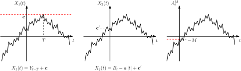
Figure 2: Illustration of the processes from Proposition 2.14 and Lemma 2.15. Left: The maximal value of $X_{1}(t)$ is $\mathbf{c}$. It is achieved at time $T$ whose law is the Lebesgue measure on $\mathbbm{R}$. Middle: On both $[0,\infty)$ and $(-\infty,0]$, the process $X_{2}(t)$ is a drifted Brownian motion starting from $\mathbf{c}^{\prime}$. Right: The process $\{A^{M}_{t}\}_{t\leq 0}$ is a drifted Brownian motion conditioned on staying below $-M$, and $\{A^{M}_{t}\}_{t\geq 0}$ is a drifted Brownian motion starting from $-M$.

Lemma 2.16.

The law of $X_{1}(0)$ in Proposition 2.14 is $\frac{1}{2a^{2}}e^{-2ac}dc$.

Proof.

We write $\mathbbm{M}_{1}$ for the measure on the sample space that generates $X_{1}$. We must show that $\mathbbm{M}_{1}[X_{1}(0)>-M]=\int_{-M}^{\infty}\frac{1}{2a^{2}}e^{-2ac}\,dc=\frac{1}{4a^{3}}e^{2aM}$ for any $M\in\mathbbm{R}$. By Lemma 2.15 and with the notations $A^{M}$ and $x$ defined there, we have

$$\mathbbm{M}_{1}[X_{1}(0)>-M\mid\mathbf{c}>-M]=\int_{\mathbbm{R}}\mathbbm{P}[A^{M}_{x+t}>-M]\,dt=\int_{\mathbbm{R}}\mathbbm{P}[A^{M}_{t}>-M]\,dt,$$

where the last equality follows from Fubini’s Theorem and the translation invariance of Lebesgue measure. For each $t>0$ we have $\mathbbm{P}[A^{M}_{t}>-M]=\mathbbm{P}[W_{t}>at]=\mathbbm{P}[Z>a\sqrt{t}]$ where $\{W_{s}:s\geq 0\}$ is standard Brownian motion and $Z\sim N(0,1)$, and for $t<0$ we a.s. have $A^{M}_{t}\leq-M$. Therefore

$$\int_{\mathbbm{R}}\mathbbm{P}[A^{M}_{t}>-M]\,dt=\int_{0}^{\infty}\int_{a\sqrt{t}}^{\infty}\frac{1}{\sqrt{2\pi}}e^{-x^{2}/2}\,dx\,dt=\int_{0}^{\infty}\frac{x^{2}}{a^{2}}\frac{1}{\sqrt{2\pi}}e^{-x^{2}/2}\,dx=\frac{1}{2a^{2}}.$$

Since $\mathbbm{M}_{1}[\mathbf{c}>-M]=\int_{-M}^{\infty}e^{-2ac}\,dc=\frac{1}{2a}e^{2aM}$, we conclude

$$\mathbbm{M}_{1}[X_{1}(0)>-M]=\mathbbm{M}_{1}[X_{1}(0)>-M\mid\mathbf{c}>-M]\mathbbm{M}_{1}[\mathbf{c}>-M]=\frac{1}{4a^{3}}e^{2aM}.\qed$$

Using Lemmas 2.15 and 2.16 we can show that the laws of $X_{1}(0)$ and $X_{2}(0)$ agree.

Proof of Proposition 2.14.

In the setting of Lemma 2.15, given $A^{M}$, let $\tau$ be sampled from Lebesgue measure on $\mathbbm{R}$. Then by Lemma 2.15, the conditional law of $\{X_{1}(t):t\in\mathbbm{R}\}$ given $\mathbf{c}>-M$ is the same as the law of $\{A^{M}_{t+\tau}:t\in\mathbbm{R}\}$. Consequently, the conditional law of $\{X_{1}(t):t\in\mathbbm{R}\}$ given $X_{1}(0)>-M$ is the same as the conditional law of $\{A^{M}_{t+\tau}:t\in\mathbbm{R}\}$ given $A^{M}_{\tau}>-M$. By definition, on the event that $A^{M}_{\tau}>-M$, we must have $\tau>0$. By the Markov property of Brownian motion, conditioning on the event that $A^{M}_{\tau}>-M$ and the value of $A^{M}_{\tau}$, the processes $\{A^{M}_{t+\tau}-A^{M}_{\tau}:t\geq 0\}$ and $\{A^{M}_{t+\tau}-A^{M}_{\tau}:t\leq 0\}$ are conditionally independent. Moreover, the conditional law of $\{A^{M}_{t+\tau}-A^{M}_{\tau}:t\geq 0\}$ equals the law of $(B_{t}-at)_{t\geq 0}$ where $B_{t}$ is a standard Brownian motion. Varying $M$, we see that conditioning on $X_{1}(0)$, the conditional law of $\{X_{1}(t)-X_{1}(0):t\geq 0\}$ and $\{X_{1}(t)-X_{1}(0):t\leq 0\}$ are conditionally independent. Moreover, the conditional law of $\{X_{1}(t)-X_{1}(0):t\geq 0\}$ equals the law of $(B_{t}-at)_{t\geq 0}$.

On the other hand, by the symmetry built into the definition of $X_{1}$, we see that $\{X_{1}(-t):t\in\mathbbm{R}\}$ has the same law as $\{X_{1}(t):t\in\mathbbm{R}\}$. Therefore conditioning on $X_{1}(0)$, the conditional law of $\{X_{1}(-t)-X_{1}(0):t\geq 0\}$ is also given by $(B_{t}-at)_{t\geq 0}$. Since by Lemma 2.16 the law of $X_{1}(0)$ is the same as $X_{2}(0)$, by the definition of $X_{2}$ we see that the law of $X_{1}$ is the same as that of $X_{2}$. ∎

Proof of Theorem 2.13.

Consider Proposition 2.14 where we have replaced $e^{-2ac}\,dc\,dt$ with $\frac{\gamma}{4}e^{-2ac}\,dc\,dt$ in the definition of $X_{1}$, and replaced $\frac{1}{2a^{2}}e^{-2ac}\,dc$ with $\frac{\gamma}{8a^{2}}e^{-2ac}\,dc$ in the definition of $X_{2}$. The proposition still holds since we are merely scaling both laws by $\frac{\gamma}{4}$. Choose $a=\frac{1}{2}(Q-\beta)$ and let $X_{1}$ and $X_{2}$ be defined as in this modified setting.

Recall $h^{1},h^{2}_{\mathcal{S}},\mathbf{c}$ from Definition 2.1 so that $\phi=h^{1}+h^{2}_{\mathcal{S}}+\mathbf{c}$. By definition, the law of $\{h^{1}(z+T)+\mathbf{c}\}_{z\in\mathcal{S}}$ equals that of $\{X_{1}(2\operatorname{Re}z)\}_{z\in\mathcal{S}}$; the prefactor $\frac{\gamma}{4}$ in $\frac{\gamma}{4}e^{-2ac}\,dc\,dt$ matches the product of $\frac{\gamma}{2}$ (from Definition 2.1) and $\frac{1}{2}$ (reparametrized Lebesgue measure in definition of $X_{1}$). Since the law of $h^{2}_{\mathcal{S}}$ is translation invariant, the law of $\{\widetilde{\phi}(z)=\phi(z+T):z\in\mathcal{S}\}$ agrees with $\{X_{1}(2\operatorname{Re}z)+h^{2}_{\mathcal{S}}(z):z\in\mathcal{S}\}$, where $h^{2}_{\mathcal{S}}$ is independently sampled from $X_{1}$.

On the other hand, by Definition 2.10, suppose $X_{2}(t)$ is independent of $h^{2}_{\mathcal{S}}$, then the law of $\{X_{2}(2\operatorname{Re}z)+h^{2}_{\mathcal{S}}(z):z\in\mathcal{C}\}$ is $\frac{\gamma}{8a^{2}}\mathrm{LF}_{\mathcal{S}}^{(\beta,\pm\infty)}$. Since $\frac{\gamma}{8a^{2}}=\frac{\gamma}{2(Q-\beta)^{2}}$, and the laws of $X_{1}$ and $X_{2}$ agree by Proposition 2.14, the law of $\widetilde{\phi}$ is $\frac{\gamma}{2(Q-\beta)^{2}}\mathrm{LF}_{\mathcal{S}}^{(\beta,\pm\infty)}$ as desired. ∎

2.4 Adding a third point to a two-pointed quantum disk

In this section we show that $\mathrm{LF}_{\mathcal{S}}^{(\beta,-\infty),(\beta,+\infty),(\gamma,0)}$ describes a two-pointed quantum disk with an additional marked point defined as follows.

Definition 2.17.

Fix $W>\frac{\gamma^{2}}{2}$. Let $(D,\phi,a,b)$ be an embedding of a sample from $\mathcal{M}_{2}^{\mathrm{disk}}(W)$ and $\nu_{\phi}$ be the quantum length measure. Let $L$ be the $\nu_{\phi}$-length of the right boundary of $(D,a,b)$, namely the counterclockwise arc from $a$ to $b$. Now suppose $(D,\phi,a,b)$ is from the reweighted measure $L\mathcal{M}_{2}^{\mathrm{disk}}(W)$. Given $\phi$, sample $\mathbf{z}$ from the probability measure proportional to the restriction of $\nu_{\phi}$ to the right boundary. We write $\mathcal{M}_{2,\bullet}^{\mathrm{disk}}(W)$ as the law of the marked quantum surface $(D,\phi,a,b,\mathbf{z})/{\sim_{\gamma}}$.

Proposition 2.18.

For $W>\frac{\gamma^{2}}{2}$, let $\phi$ be sampled from $\frac{\gamma}{2(Q-\beta)^{2}}\mathrm{LF}_{\mathcal{S}}^{(\beta,-\infty),(\beta,+\infty),(\gamma,0)}$ where $\beta=\gamma+\frac{2}{\gamma}-\frac{W}{\gamma}$. Then $(\mathcal{S},\phi,-\infty,+\infty,0)/{\sim_{\gamma}}$ is a sample from $\mathcal{M}_{2,\bullet}^{\mathrm{disk}}(W)$.

Remark 2.19.

Our $\mathcal{M}_{2,\bullet}^{\mathrm{disk}}(2)$ equals $\mathrm{QD}_{0,3}$ restricted to the event $E$ that the three boundary points are in the clockwise order. Setting $\alpha=\gamma$ in Proposition 2.18 and using the change of coordinate from Proposition 2.7 and Lemma 2.11 gives the following. Suppose $(\mathbbm{H},\phi,s_{1},s_{2},s_{3})$ is an embedding of $\mathrm{QD}_{0,3}|_{E}$, where $s_{1},s_{2},s_{3}$ are three fixed distinct clockwise-oriented points on $\partial\mathbbm{H}$. Then the law of $\phi$ is $C\mathrm{LF}_{\mathbbm{H}}^{(\gamma,s_{1}),(\gamma,s_{2}),(\gamma,s_{3})}$ with $C=\frac{\gamma}{2(Q-\gamma)^{2}}$. The main result of [Cer19] is equivalent to this statement without identifying $C$. We can also recover the result of [AHS17] on $\mathrm{QS}_{3}$, see Proposition 2.26.

To prove Proposition 2.18, we start with an infinite-measure variant of the rooted measure in LQG. The argument via Girsanov’s theorem is standard we give the full detail as variants of it will be used repeatedly. In the statement we recall Remark 2.3 that $P_{\mathcal{S}}$ is understood as a measure on $H^{-1}(\mathcal{S})$. Moreover, we write $\mathbbm{E}_{\mathcal{S}}$ as the expectation over $P_{\mathcal{S}}$.

Lemma 2.20.

Let $Q(dh,du)=\nu_{h}(du)P_{\mathcal{S}}(dh)$ for $(h,u)\in H^{-1}(\mathcal{S})\times\mathbbm{R}$. Namely, $Q$ is the (infinite) measure on $H^{-1}(\mathcal{S})\times\mathbbm{R}$ such that for non-negative measurable functions $f$ on $H^{-1}(\mathcal{S})$ and $g$ on $\mathbbm{R}$ we have

$$\int f(h)g(u)\,Q(dh,du)=\int f(h)\mathopen{}\mathclose{{}\left(\int_{\mathbbm{R}}g(u)\nu_{h}(du)}\right)\,P_{\mathcal{S}}(dh).$$

Let $\rho$ be such that $\rho(u)du=\mathbbm{E}_{\mathcal{S}}[\nu_{h}(du)]$ with the latter measure defined in Lemma 2.12. Then

$$\int f(h)g(u)\,Q(dh,du)=\int_{\mathbbm{R}}\mathbbm{E}_{\mathcal{S}}\mathopen{}\mathclose{{}\left[f(h+\frac{\gamma}{2}G_{\mathcal{S}}(\cdot,u))}\right]g(u)\rho(u)\,du.$$

Proof.

It suffices to assume that $g$ is a compactly supported continuous function on $\mathbbm{R}$ and $f$ is a bounded and continuous function on $H^{-1}(\mathcal{S})$. For $\varepsilon>0$, let $\nu_{h,\varepsilon}(dx)=\varepsilon^{\gamma^{2}/4}e^{\frac{\gamma}{2}h_{\varepsilon}(x)}dx$. Since $\lim\limits_{\varepsilon\to 0}\int_{\mathbbm{R}}g(u)\,\nu_{h,\varepsilon}(du)=\int_{\mathbbm{R}}g(u)\,\nu_{h}(du)$ in $L^{1}$ with respect to $P_{\mathcal{S}}$ (see e.g. [Ber17, Theorem 1.1]), we have

$$\begin{split}\lim_{\varepsilon\to 0}\int f(h)\mathopen{}\mathclose{{}\left(\int_{\mathbbm{R}}g(u)\,\nu_{h,\varepsilon}(du)}\right)\,P_{\mathcal{S}}(dh)&=\int f(h)\mathopen{}\mathclose{{}\left(\int_{\mathbbm{R}}g(u)\,\nu_{h}(du)}\right)\,P_{\mathcal{S}}(dh)\\ &=\int f(h)g(u)\,Q(dh,du).\end{split}$$ (2.5)

Let $G_{\mathcal{S},\varepsilon}(z,u)=\mathbbm{E}_{\mathcal{S}}[h(z)h^{\varepsilon}(u)]$, where the latter is understood via the $\varepsilon$-circle average of $G_{\mathcal{S}}(z,)$. By Girsanov’s theorem, the left side of (2.5) equals

$$\int_{\mathbbm{R}}\mathbbm{E}_{\mathcal{S}}\mathopen{}\mathclose{{}\left[f(h+\frac{\gamma}{2}G_{\mathcal{S},\varepsilon}(\cdot,u))}\right]g(u)\mathbbm{E}_{\mathcal{S}}[\varepsilon^{\gamma^{2}/4}e^{\frac{\gamma}{2}h_{\varepsilon}(u)}]\,du.$$

Since $\rho(u)du=\lim\limits_{\varepsilon\to 0}\mathbbm{E}_{\mathcal{S}}[\varepsilon^{\gamma^{2}/4}e^{\frac{\gamma}{2}h_{\varepsilon}(u)}]du$ and $\lim_{\varepsilon\to 0}G_{\mathcal{S},\varepsilon}(\cdot,u)=G_{\mathcal{S}}(\cdot,u)$ in $H^{-1}(\mathcal{S})$, we get the desired result. ∎

The following lemma is a variant of Lemma 2.20 for Liouville fields. For notational convenience we use the notion $M[f(\phi)]=\int f(\phi)M(d\phi)$.

Lemma 2.21.

Let $\mathrm{LF}_{\mathcal{S}}^{(\beta,\pm\infty),(\beta_{j},s_{j})_{j}}$ be as in Definition 2.10. Let $f$ and $g$ be non-negative measurable functions as in Lemma 2.20. Then

$$\mathrm{LF}_{\mathcal{S}}^{(\beta,\pm\infty)}\mathopen{}\mathclose{{}\left[f(\phi)\int_{\mathbbm{R}}g(u)\nu_{\phi}\,(du)}\right]=\int_{\mathbbm{R}}\mathrm{LF}_{\mathcal{S}}^{(\beta,\pm\infty),(\gamma,u)}[f(\phi)]g(u)\,du.$$ (2.6)

Proof.

By Definition 2.10 the left side of (2.6) can be written as

$$\iint f(h-(Q-\beta)\mathopen{}\mathclose{{}\left|\operatorname{Re}\cdot}\right|+c)\mathopen{}\mathclose{{}\left(\int_{\mathbbm{R}}g(u)e^{\frac{\gamma}{2}\mathopen{}\mathclose{{}\left(-(Q-\beta)\mathopen{}\mathclose{{}\left|\operatorname{Re}u}\right|+c}\right)}\,\nu_{h}(du)}\right)\,P_{\mathcal{S}}(dh)e^{(\beta-Q)c}\,dc.$$

By Lemma 2.20, the integration over $P_{\mathcal{S}}$ with a fixed $c$ is given by

$$\iint f(h+\frac{\gamma}{2}G_{\mathcal{S}}(\cdot,u)-(Q-\beta)\mathopen{}\mathclose{{}\left|\operatorname{Re}\cdot}\right|+c)g(u)e^{\frac{\gamma}{2}(-(Q-\beta)\mathopen{}\mathclose{{}\left|\operatorname{Re}u}\right|+c)}\rho(u)\cdot e^{(\beta-Q)c}P_{\mathcal{S}}(dh)du$$ (2.7)

where $\rho(u)$ is as in Lemma 2.20. Recall $C^{(\beta,\pm\infty),(\gamma,u)}_{\mathcal{S}}$ in the definition of $\mathrm{LF}_{\mathcal{S}}^{(\beta,\pm\infty),(\gamma,u)}$. By Lemma 2.12 we have

$$C^{(\beta,\pm\infty),(\gamma,u)}_{\mathcal{S}}du=e^{\frac{\gamma}{2}(-(Q-\beta)\mathopen{}\mathclose{{}\left|\operatorname{Re}u}\right|)}\rho(u)du.$$

Therefore the integral in (2.7) becomes

$$\iint f(h-(Q-\beta)\mathopen{}\mathclose{{}\left|\operatorname{Re}\cdot}\right|+\frac{\gamma}{2}G_{\mathcal{S}}(\cdot,u)+c)g(u)e^{\frac{\gamma}{2}c}\cdot e^{(\beta-Q)c}\cdot C^{(\beta,\pm\infty),(\gamma,u)}_{\mathcal{S}}P_{\mathcal{S}}(dh)du.$$

Further integrating over $c$ we get $\int_{\mathbbm{R}}\mathrm{LF}_{\mathcal{S}}^{(\beta,\pm\infty),(\gamma,u)}[f(\phi)]g(u)\,du$ as desired. ∎

Proof of Proposition 2.18.

Our proof is based on Theorem 2.13 and (2.6). For $u\in\mathbbm{R}$, let $M^{u}_{\bullet}$ be such that $(\mathcal{S},\phi,-\infty+\infty,u)/{\sim_{\gamma}}$ is a sample from $\mathcal{M}_{2,\bullet}^{\mathrm{disk}}$ if $\phi$ is a sample from $M^{u}_{\bullet}$. We must show that $M^{0}_{\bullet}=\frac{\gamma}{2(Q-\beta)^{2}}\mathrm{LF}_{\mathcal{S}}^{(\beta,\pm\infty),(\gamma,0)}$.

Let $M_{0}$ be the law of $\phi$ in Definition 2.1 where $(\mathcal{S},\phi,+\infty,-\infty)/{\sim_{\gamma}}$ is a sample from $\mathcal{M}_{2}^{\mathrm{disk}}(W)$. Let $Q_{0}$ be the measure on $\{(\phi,z):h\textrm{ is a distribution on }\mathcal{S},u\in\mathbbm{R}\}$ such that for non-negative measurable functions $f$ and $g$ we have

$$\int f(\phi)g(z)\,Q_{0}(d\phi,dz)=\int f(\phi)\mathopen{}\mathclose{{}\left(\int_{\mathbbm{R}}g(z)\,\nu_{\phi}(dz)}\right)\,M_{0}(d\phi).$$

Then the $Q_{0}$-law of $(\mathcal{S},\phi,-\infty,+\infty,z)/{\sim_{\gamma}}$ is $\mathcal{M}_{2,\bullet}^{\mathrm{disk}}(W)$. Let $(\phi,\mathbf{z})$ and $T$ be sampled from $Q_{0}\times dt$, where $dt$ is the Lebesgue measure on $\mathbbm{R}$. Set $\mathbf{u}=\mathbf{z}-T$ and $\widetilde{\phi}(\cdot)=\phi(\cdot+T)$. Let $M$ be the law of $(\widetilde{\phi},\mathbf{u})$. Then by definition

$$M[f(\widetilde{\phi})g(u)]=\int_{\mathbbm{R}}M^{u}_{\bullet}[f(\widetilde{\phi})]g(u)\,du.$$ (2.8)

On the other hand, note that the $\nu_{\phi}(\mathbbm{R})^{-1}Q_{0}$-law of $\phi$ is $M_{0}$. Therefore, by Theorem 2.13, the law of $\widetilde{\phi}$ under $\nu_{\widetilde{\phi}}(\mathbbm{R})^{-1}M$ is $\frac{\gamma}{2(Q-\beta)^{2}}\mathrm{LF}_{\mathcal{S}}^{(\beta,\pm\infty)}$. Moreover, conditioning on $\widetilde{\phi}$, the conditional law of $\mathbf{u}$ is the probability measure proportional to $\nu_{\widetilde{\phi}}|_{\mathbbm{R}}$. Therefore,

$$M[f(\widetilde{\phi})g(u)]=\frac{\gamma}{2(Q-\beta)^{2}}\mathrm{LF}_{\mathcal{S}}^{(\beta,\pm\infty)}\mathopen{}\mathclose{{}\left[f(\widetilde{\phi})\int_{\mathbbm{R}}g(u)\,\nu_{\widetilde{\phi}}(du)}\right].$$

By Lemma 2.21, we have

$$M[f(\widetilde{\phi})g(u)]=\frac{\gamma}{2(Q-\beta)^{2}}\int_{\mathbbm{R}}\mathrm{LF}_{\mathcal{S}}^{(\beta,\pm\infty),(\gamma,u)}[f(\phi)]g(u)\,du.$$ (2.9)

Combining (2.8) and (2.9) we get $M^{u}_{\bullet}[f(\widetilde{\phi})]=\frac{\gamma}{2(Q-\beta)^{2}}\mathrm{LF}_{\mathcal{S}}^{(\beta,\pm\infty),(\gamma,u)}[f(\widetilde{\phi})]$, since $g$ can be arbitrary. Setting $u=0$ and varying $f$ we conclude the proof. ∎

2.5 Uniform embedding of the quantum sphere and quantum disk

With notation as in Section 1.2, Theorem 2.13 says that the uniform embedding of $\mathcal{M}_{2}^{\mathrm{disk}}(W)$ in $(\mathcal{S},-\infty,+\infty)$ is given by a constant multiple of $\mathrm{LF}_{\mathcal{S}}^{(\beta,\pm\infty)}$. More precisely

$$\begin{split}&\mathbf{m}_{\mathcal{S},-\infty,+\infty}\ltimes\mathcal{M}_{2}^{\mathrm{disk}}(W)=\frac{\gamma}{2(Q-\beta)^{2}}\mathrm{LF}_{\mathcal{S}}^{(\beta,\pm\infty)},\qquad\beta=Q+\frac{\gamma}{2}-\frac{W}{\gamma}.\end{split}$$

It is in fact a general phenomenon that uniform embedding of random surfaces appearing in the framework of [DMS14] are given by a Liouville field. In this section we demonstrate this point by proving Theorem 1.2, which concerns the uniform embedding of the quantum sphere and disk. Unlike the rest of the paper, which focuses on LQG surfaces with disk topology, in this subsection we treat the sphere and disk in parallel.

We first give a precise definition of the notation $\ltimes$ that represents uniform embedding. Let $G$ be a locally compact Lie group. Suppose $\Omega$ is a Polish space with a continuous $G$-action $(g,x)\mapsto g\cdot x$. Namely, $g_{1}\cdot(g_{2}\cdot x)=(g_{1}\cdot g_{2})\cdot x$ for all $g_{1},g_{2}\in G$ and $x\in\Omega$; moreover, $(g,x)\mapsto g\cdot x$ is continuous. Let $\Omega/G$ be such that $y\in\Omega/G$ if and only if $y=\{gx:g\in G\}$ for some $x\in\Omega$. We let $\pi:\Omega\rightarrow\Omega/G$ be the quotient map and endow $\Omega/G$ with the quotient topology. We endow the Borel $\sigma$-algebra on $G,\Omega$ and $\Omega/G$. Suppose $\mathbf{m}$ is a right invariant Haar measure. That is, $\int_{G}f(gh)\,\mathbf{m}(dg)=\int_{G}f(g)\,\mathbf{m}(dg)$ for each non-negative measurable function $f$ on $G$ and each $h\in G$.

Definition 2.22.

For each $y\in\Omega/G$, choose $x\in\pi^{-1}(y)$. We write $\mathbf{m}\ltimes y$ for the pushforward measure of $\mathbf{m}$ under $G\ni g\mapsto g\cdot x\in\Omega$, i.e. for each Borel $E\subset\Omega$ we have $\mathbf{m}\ltimes y(E)=\int_{\Omega}1_{g\cdot x\in E}\mathbf{\,}m(dg)$. For a $\sigma$-finite measure $\widetilde{\nu}$ on $\Omega/G$, we write the measure $\int_{\Omega/G}[\mathbf{m}\ltimes y]\,\widetilde{\nu}(dy)$ as $\mathbf{m}\ltimes\widetilde{\nu}$. Namely, $\mathbf{m}\ltimes\widetilde{\nu}(E)=\int_{\Omega/G}[\mathbf{m}\ltimes y](E)\,\widetilde{\nu}(dy)$ for each Borel set $E\subset\Omega$.

Lemma 2.23.

For each $\sigma$-finite measure $\nu$ on $\Omega$, let $\pi_{*}\nu$ be the pushforward of $\nu$ by $\pi$. Then the pushforward of $\mathbf{m}\times\nu$ under $(g,x)\mapsto g\cdot x$ equals $\mathbf{m}\ltimes\pi_{*}\nu$.

Proof.

For each non-negative continuous function $f$ on $\Omega$, let $I_{f}(x)=\int_{G}f(g\cdot x)\,\mathbf{m}(dg)$. Since $\mathbf{m}$ is right invariant, $I_{f}(x)$ only depends on $\pi(x)$. Equivalently, there exists a non-negative continuous function $\widetilde{I}_{f}$ on $\Omega/G$ such that $I_{f}=\widetilde{I}_{f}\circ\pi$. For each $\sigma$-finite measure $\nu$ on $(\Omega,\mathcal{F})$, by Fubini’s Theorem,

$$\int_{G\times\Omega}f(g\cdot x)\,\mathbf{m}(dg)\nu(dx)=\int_{\Omega}I_{f}(x)\,\nu(dx)=\int_{\Omega/G}\widetilde{I}_{f}(y)\,\pi_{*}\nu(dy).$$ (2.10)

The last integral in (2.10) is precisely $\int_{\Omega/G}\mathopen{}\mathclose{{}\left(\int f(x^{\prime})\,\mathbf{m}\ltimes y(dx^{\prime})}\right)\,\pi_{*}\nu(dy)$. This concludes the proof. ∎

The proof of Theorem 1.2 relies on the LCFT description of the three-pointed quantum disk $\mathrm{QD}_{0,3}$ and sphere $\mathrm{QS}_{3}$. The description of $\mathrm{QD}_{0,3}$ was obtained in [Cer19] which we recovered and refined in Proposition 2.18 and Remark 2.19. In Appendix B, following the same proof we recover and refine the LCFT description of $\mathrm{QS}_{3}$ obtained in [AHS17]. In particular, we prove a more general result (Proposition B.7) in analogy to Proposition 2.18. The original definition of $\mathrm{QS}_{3}$ is recalled in Appendix B but the LCFT description in Proposition 2.26 is what we need for the rest of this section. The unpointed quantum sphere $\mathrm{QS}$ in Theorem 1.2 can be obtained by deweighting the cubic power of the total quantum area of a sample from $\mathrm{QS}_{3}$ and forgetting the three marked points; see Definition B.2.

We first recall the basic setup of LCFT on $\mathbbm{C}$ following [DKRV16, KRV20, Var17], and then state the LCFT description of $\mathrm{QS}_{3}$ as Proposition 2.26 (see Appendix B for the proof). Let $P_{\mathbbm{C}}$ be the law of the GFF on $\mathbbm{C}$ normalized to have average zero on the unit circle, which has covariance kernel (see [KRV20, (2.1), Remark 2.1])

$$G_{\mathbbm{C}}(z,w) =-\log|z-w|+\log|z|_{+}+\log|w|_{+}.$$

Definition 2.24.

Let $(h,\mathbf{c})$ be sampled from $P_{\mathbbm{C}}\times[e^{-2Qc}dc]$ and set $\phi=h(z)-2Q\log|z|_{+}+\mathbf{c}$. We write $\mathrm{LF}_{\mathbbm{C}}$ as the law of $\phi$ and call a sample from $\mathrm{LF}_{\mathbbm{C}}$ a Liouville field on $\mathbbm{C}$.

Definition 2.25.

Let $(\alpha_{i},z_{i})\in\mathbbm{R}\times\mathbbm{C}$ for $i=1,\dots,m$, where $m\geq 1$ and the $z_{i}$ are distinct. Let $(h,\mathbf{c})$ be sampled from $C_{\mathbbm{C}}^{(\alpha_{i},z_{i})_{i}}P_{\mathbbm{C}}\times[e^{(\sum_{i}\alpha_{i}-2Q)c}dc]$ where

$$C_{\mathbbm{C}}^{(\alpha_{i},z_{i})_{i}}=\prod_{i=1}^{m}|z_{i}|_{+}^{-\alpha_{i}(2Q-\alpha_{i})}e^{\sum_{j=i+1}^{m}\alpha_{i}\alpha_{j}G_{\mathbbm{C}}(z_{i},z_{j})}.$$

Let $\phi(z)=h(z)-2Q\log|z|_{+}+\sum_{i=1}^{m}\alpha_{i}G_{\mathbbm{C}}(z,z_{i})+\mathbf{c}$. We write $\mathrm{LF}_{\mathbbm{C}}^{(\alpha_{i},z_{i})_{i}}$ for the law of $\phi$ and call a sample from $\mathrm{LF}_{\mathbbm{C}}^{(\alpha_{i},z_{i})_{i}}$ the Liouville field on $\mathbbm{C}$ with insertions $(\alpha_{i},z_{i})_{1\leq i\leq m}$.

Proposition 2.26.

Suppose $(\mathbbm{C},\phi,u_{1},u_{2},u_{3})$ is an embedding of $\mathrm{QS}_{3}$, where $u_{1},u_{2},u_{3}$ are three fixed distinct points on $\mathbbm{C}$. Then the law of $\phi$ is $\frac{\pi\gamma}{2(Q-\gamma)^{2}}\mathrm{LF}_{\mathbbm{C}}^{(\gamma,u_{1}),(\gamma,u_{2}),(\gamma,u_{3})}$.

To make sense of $\mathbf{m}_{\widehat{\mathbbm{C}}}\ltimes\mathrm{QS}$, consider the function space $H^{-1}(\mathbbm{C})$ defined as $H^{-1}(\mathbbm{H})$ in Remark 2.3 with $\mathbbm{C}$ in place of $\mathbbm{H}$. The conformal coordinate change $f\bullet_{\gamma}\phi=\phi\circ f^{-1}+Q\log\mathopen{}\mathclose{{}\left|(f^{-1})^{\prime}}\right|$ defines a continuous group action of $\operatorname{conf}(\widehat{\mathbbm{C}})$ on $H^{-1}(\mathbbm{C})$, where $\operatorname{conf}(\widehat{\mathbbm{C}})$ is conformal automorphism group on $\widehat{\mathbbm{C}}$. By the definition of quantum surface, we can view $\mathrm{QS}$ as a measure on $H^{-1}(\mathbbm{C})/\operatorname{conf}(\widehat{\mathbbm{C}})$. Since $\operatorname{conf}(\widehat{\mathbbm{C}})$ is a locally compact Lie group, it has a unique right invariant Haar measure modulo a multiplicative constant, and moreover, the measure is left invariant as well since $\operatorname{conf}(\widehat{\mathbbm{C}})$ is unimodular; (see e.g. [Far08, Corollary 5.5.5]). From Definition 2.22, we get the precise meaning of $\mathbf{m}_{\widehat{\mathbbm{C}}}\ltimes\mathrm{QS}$. The uniform embedding $\mathbf{m}_{\mathbbm{H}}\ltimes\mathrm{QD}$ of $\mathrm{QD}$ is defined in the same way.

The starting point of the proof of Theorem 1.2 is the LCFT description of the uniform embedding of $\mathrm{QS}_{3}$ and $\mathrm{QD}_{0,3}$ instead of $\mathrm{QS}$ and $\mathrm{QD}$. To make sense of $\mathbf{m}_{\widehat{\mathbbm{C}}}\ltimes\mathrm{QS}_{3}$, we view $\mathrm{QS}_{3}$ as a measure on the quotient space of $\Omega_{\mathbbm{C}}\times\mathbbm{C}^{3}$ under the $\operatorname{conf}(\widehat{\mathbbm{C}})$-action $(h,a,b,c)\mapsto(f\bullet_{\gamma}h,f(a),f(b),f(c))$. Then $\mathbf{m}_{\widehat{\mathbbm{C}}}\ltimes\mathrm{QS}_{3}$ is a measure on $\Omega_{\mathbbm{C}}\times\mathbbm{C}^{3}$. We similarly define $\mathbf{m}_{\widehat{\mathbbm{C}}}\ltimes\mathrm{QS}_{3}$. The following lemma gives a concrete realization of $\mathbf{m}_{\mathbbm{H}}\ltimes\mathrm{QD}_{0,3}$ and $\mathbf{m}_{\widehat{\mathbbm{C}}}\ltimes\mathrm{QS}_{3}$.

Lemma 2.27.

Let $(\mathbb{\mathbbm{C}},\phi,a,b,c)$ be an embedding of a sample from $\mathrm{QS}_{3}$. Let $\mathfrak{f}$ be a sample from a Haar measure $\mathbf{m}_{\widehat{\mathbbm{C}}}$ on $\operatorname{conf}(\widehat{\mathbbm{C}})$ that is independent of $(\phi,a,b,c)$. Then the law of $(\mathfrak{f}\bullet_{\gamma}\phi,\mathfrak{f}(a),\mathfrak{f}(b),\mathfrak{f}(c))$ is $\mathbf{m}_{\widehat{\mathbbm{C}}}\ltimes\mathrm{QS}_{3}$. In particular, it does not depend on the law of $(\phi,a,b,c)$. Similarly, let $(\mathbbm{H},\phi,a,b,c)$ be an embedding of a sample from $\mathrm{QD}_{0,3}$, and $\mathfrak{g}$ an independent sample from a Haar measure $\mathbf{m}_{\mathbbm{H}}$ on $\mathrm{conf}(\mathbbm{H})$. Then the law of $(\mathfrak{g}\bullet_{\gamma}\phi,\mathfrak{g}(a),\mathfrak{g}(b),\mathfrak{g}(c))$ is $\mathbf{m}_{\mathbbm{H}}\ltimes\mathrm{QD}_{0,3}$.

Proof.

This immediately follows from Lemma 2.23. ∎

We now give an explicit description of $\mathbf{m}_{\widehat{\mathbbm{C}}}$ and $\mathbf{m}_{\mathbbm{H}}$.

Lemma 2.28.

Let $\mathfrak{f}$ be sampled from a Haar measure $\mathbf{m}_{\widehat{\mathbbm{C}}}$ of $\operatorname{conf}(\widehat{\mathbbm{C}})$. Then there exists a constant $C\in(0,\infty)$ such that the law of $(\mathfrak{f}(0),\mathfrak{f}(1),\mathfrak{f}(-1))$ is $C|(p-q)(q-r)(r-p)|^{-2}\,d^{2}p\,d^{2}q\,d^{2}r$.

Similarly, let $\mathfrak{g}$ be sampled from a Haar measure $\mathbf{m}_{\mathbbm{H}}$ of $\operatorname{conf}(\mathbbm{H})$. Then there exists a constant $C\in(0,\infty)$ such that the law of $(\mathfrak{g}(0),\mathfrak{g}(1),\mathfrak{g}(-1))$ is $C|(p-q)(q-r)(r-p)|^{-1}\,dp\,dq\,dr$ restricted to the set of triples $(p,q,r)\in\mathbbm{R}^{3}$ that are counterclockwise aligned on $\partial\mathbbm{H}$.

Proof.

We prove the first assertion; the second follows from the same arguments. By the uniqueness of Haar measure, it suffices to show that if $(\mathbf{p},\mathbf{q},\mathbf{r})$ is sampled from $|(p-q)(q-r)(r-p)|^{-2}\,d^{2}p\,d^{2}q\,d^{2}r$ and $\mathfrak{f}$ is the unique Mobius transformation mapping $(0,1,-1)$ to $(\mathbf{p},\mathbf{q},\mathbf{r})$, then the law of $\mathfrak{f}$ is a Haar measure on $\operatorname{conf}(\widehat{\mathbbm{C}})$. Namely for each $g\in\operatorname{conf}(\widehat{\mathbbm{C}})$, $g\circ\mathfrak{f}$ agrees in law with $\mathfrak{f}$. This is equivalent to the statement that $(g(\mathbf{p}),g(\mathbf{q}),g(\mathbf{r}))$ agrees in law with $(\mathbf{p},\mathbf{q},\mathbf{r})$. This is straightforward to check when $g$ is a translation, dilation, or inversion. Since these generate $\operatorname{conf}(\widehat{\mathbbm{C}})$, we are done. ∎

We will give the LCFT description of $\mathbf{m}_{\widehat{\mathbbm{C}}}\ltimes\mathrm{QS}_{3}$ and $\mathbf{m}_{\mathbbm{H}}\ltimes\mathrm{QD}_{0,3}$ in Proposition 2.30 below. In its proof we need Proposition 2.7 and its sphere counterpart, which we recall now.

Proposition 2.29 ([DKRV16, Theorem 3.5]).

For $\alpha\in\mathbbm{R}$, set $\Delta_{\alpha}:=\frac{\alpha}{2}(Q-\frac{\alpha}{2})$. Let $f\in\operatorname{conf}(\widehat{\mathbbm{C}})$ and $(\alpha_{i},z_{i})\in\mathbbm{R}\times\mathbbm{C}$ be such that $f(z_{i})\neq\infty$ for all $1\leq i\leq m$. Recall the notation $f_{*}$ in Proposition 2.7. Then

$$\mathrm{LF}_{\mathbbm{C}}=f_{*}\mathrm{LF}_{\mathbbm{C}}\quad\textrm{and}\quad\mathrm{LF}_{\mathbbm{C}}^{(\alpha_{i},f(z_{i}))_{i}}=\prod_{i=1}^{m}|f^{\prime}(z_{i})|^{-2\Delta_{\alpha_{i}}}f_{*}\mathrm{LF}_{\mathbbm{C}}^{(\alpha_{i},z_{i})_{i}}.$$

Proposition 2.30.

Suppose the Haar measures $\mathbf{m}_{\widehat{\mathbbm{C}}},\mathbf{m}_{\mathbbm{H}}$ are such that the constant $C$ in Lemma 2.28 is equal to 1. Then for non-negative measurable functions $f$ and $g$ on $H^{-1}(\mathbbm{C})$ and $\mathbbm{C}^{3}$, respectively,

$$\begin{split}&\mathbf{m}_{\widehat{\mathbbm{C}}}\ltimes\mathrm{QS}_{3}[f(\phi)g(p,q,r)]\\ &\qquad=\frac{\pi\gamma}{2(Q-\gamma)^{2}}\int_{\mathbbm{C}^{3}}\mathrm{LF}_{\mathbbm{C}}^{(\gamma,p),(\gamma,q),(\gamma,r)}[f(\phi)]g(p,q,r)\,d^{2}p\,d^{2}q\,d^{2}r,\end{split}$$ (2.11)

and for non-negative measurable functions $f$ and $g$ on $H^{-1}(\mathbbm{H})$ and $\mathbbm{R}^{3}$, respectively,

$$\begin{split}&\mathbf{m}_{\mathbbm{H}}\ltimes\mathrm{QD}_{0,3}[f(\phi)g(p,q,r)]\\ &\qquad=\frac{\gamma}{2(Q-\gamma)^{2}}\int_{\mathbbm{R}^{3}}\mathrm{LF}_{\mathbbm{H}}^{(\gamma,p),(\gamma,q),(\gamma,r)}[f(\phi)]g(p,q,r)\,dp\,dq\,dr.\end{split}$$ (2.12)

Proof.

We prove (2.11); the proof of (2.12) is similar. In Lemma 2.27, we choose $(a,b,c)=(0,1,-1)$. By Proposition B.7, the law of $\phi$ is $\frac{2\pi\gamma}{(Q-\gamma)^{2}}\cdot\mathrm{LF}_{\mathbbm{C}}^{(\gamma,0),(\gamma,1),(\gamma,-1)}$. Given three distinct points $p,q,r$ in $\mathbbm{C}^{3}$. Suppose $f\in\operatorname{conf}(\widehat{\mathbbm{C}})$ maps $(0,1,-1)$ to $(p,q,r)$. Then we can explicit get $f(z)=\frac{(pq-2qr+rp)z+p(q-r)}{(2p-q-r)z+q-r}$ and

$$\begin{split}&f^{\prime}(0)=\frac{2(p-q)(q-r)(r-p)}{(q-r)^{2}},\qquad f^{\prime}(1)=\frac{2(p-q)(q-r)(r-p)}{4(r-p)^{2}},\\ &f^{\prime}(-1)=\frac{2(p-q)(q-r)(r-p)}{4(p-q)^{2}}.\end{split}$$ (2.13)

Recall notations from Proposition 2.29. Since $\Delta_{\gamma}=1$, we have

$$\begin{split}f_{*}\mathrm{LF}_{\mathbbm{C}}^{(\gamma,0),(\gamma,1),(\gamma,-1)}&=|f^{\prime}(0)f^{\prime}(1)f^{\prime}(-1)|^{2}\mathrm{LF}_{\mathbbm{C}}^{(\gamma,p),(\gamma,q),(\gamma,r)}\\ &=C|(p-q)(q-r)(r-p)|^{2}\mathrm{LF}_{\mathbbm{C}}^{(\gamma,p),(\gamma,q),(\gamma,r)}.\end{split}$$

Since the law of $(\mathfrak{f}(0),\mathfrak{f}(1),\mathfrak{f}(-1))$ is $|(p-q)(q-r)(r-p)|^{-2}\,d^{2}p\,d^{2}q\,d^{2}r$, and $\mathbf{m}_{\widehat{\mathbbm{C}}}\ltimes\mathrm{QS}_{3}$ describes the law of $(\mathfrak{f}\bullet_{\gamma}\phi,\mathfrak{f}(0),\mathfrak{f}(1),\mathfrak{f}(-1))$, we obtain (2.11). ∎

To pass from the uniform embedding of $\mathrm{QD}_{0,3}$ and $\mathrm{QS}_{3}$ to that of $\mathrm{QD}$ and $\mathrm{QS}$, we need Lemma 2.21 and its sphere counterpart, which we state below and prove in Appendix B.

Lemma 2.31.

We have

$$\mathrm{LF}_{\mathbbm{C}}^{(\alpha_{i},z_{i})_{i}}\mathopen{}\mathclose{{}\left[f(\phi)\int_{\mathbbm{C}}g(u)\,\mu_{\phi}(du)}\right]=\int_{\mathbbm{C}}\mathrm{LF}_{\mathbbm{C}}^{(\alpha_{i},z_{i})_{i},(\gamma,u)}[f(\phi)]g(u)\,d^{2}u.$$

for non-negative measurable functions $f$ and $g$.

Proposition 2.32.

Suppose the Haar measures $\mathbf{m}_{\widehat{\mathbbm{C}}},\mathbf{m}_{\mathbbm{H}}$ are such that the constant $C$ in Lemma 2.28 is equal to 1, then

$$\mathbf{m}_{\widehat{\mathbbm{C}}}\ltimes\mathrm{QS}=\frac{\pi\gamma}{2(Q-\gamma)^{2}}\mathrm{LF}_{\mathbbm{C}}\quad\text{ and }\quad\mathbf{m}_{\mathbbm{H}}\ltimes\mathrm{QD}=\frac{\gamma}{2(Q-\gamma)^{2}}\mathrm{LF}_{\mathbbm{H}}.$$

Proof.

Repeatedly applying Lemma 2.31, we get

$$\begin{split}&\mathrm{LF}_{\mathbbm{C}}\mathopen{}\mathclose{{}\left[f(\phi)\int_{\mathbbm{C}^{3}}g(p,q,r)\mu_{\phi}(dp)\mu_{\phi}(dq)\mu_{\phi}(dr)}\right]\\ &\qquad\qquad=\int_{\mathbbm{C}^{3}}\mathrm{LF}_{\mathbbm{C}}^{(\gamma,p),(\gamma,q),(\gamma,r)}[f(\phi)]g(p,q,r)\,d^{2}p\,d^{2}q\,d^{2}r.\end{split}$$ (2.14)

Setting $g=1$ in Proposition 2.30 and (2.14), we have $\mathbf{m}_{\widehat{\mathbbm{C}}}\ltimes\mathrm{QS}_{3}[f(\phi)]=\frac{\pi\gamma}{2(Q-\gamma)^{2}}\mathrm{LF}_{\mathbbm{C}}\mathopen{}\mathclose{{}\left[f(\phi)\mu_{\phi}(\mathbbm{C})^{3}}\right]$. By the definition of $\mathbf{m}_{\widehat{\mathbbm{C}}}\ltimes\mathrm{QS}_{3}$ in Lemma 2.27 the marginal law of the field under $\mathbf{m}_{\widehat{\mathbbm{C}}}\ltimes\mathrm{QS}_{3}$ is $\mu_{\phi}(\mathbbm{C})^{3}\mathbf{m}_{\widehat{\mathbbm{C}}}\ltimes\mathrm{QS}$. Therefore $\mathbf{m}_{\widehat{\mathbbm{C}}}\ltimes\mathrm{QS}=\frac{\pi\gamma}{2(Q-\gamma)^{2}}\mathrm{LF}_{\mathbbm{C}}$. The proof of $\mathbf{m}_{\mathbbm{H}}\ltimes\mathrm{QD}=\frac{\gamma}{2(Q-\gamma)^{2}}\mathrm{LF}_{\mathbbm{H}}$ is identical. ∎

Proof of Theorem 1.2.

This follows from Proposition 2.32 by the uniqueness of Haar measure modulo multiplication by a constant. ∎

Our proof of Theorem 1.2 demonstrates how to go from $\mathrm{QS}_{3}=C\mathrm{LF}_{\mathbbm{C}}^{(\gamma,0),(\gamma,1),(\gamma,-1)}$ to $\mathbf{m}_{\widehat{\mathbbm{C}}}\ltimes\mathrm{QS}=C\mathrm{LF}_{\mathbbm{C}}$ through Proposition 2.30 and de-weighting. Similar arguments can also give results such as $\mathbf{m}_{\widehat{\mathbbm{C}},0}\ltimes\mathrm{QS}_{1}=C\mathrm{LF}_{\mathbbm{C}}^{(\gamma,0)}$, where $\mathbf{m}_{\widehat{\mathbbm{C}},0}$ is a Haar measure on the subgroup of $\operatorname{conf}(\widehat{\mathbbm{C}})$ fixing $0$. We do not need these statements so we omit the details.

3 Quantum surface and Liouville correlation function

In this section we consider disks with two or three marked boundary points and we derive the law of boundary lengths of these surfaces. More specifically, we consider surfaces sampled from $\mathcal{M}_{0,2}^{\mathrm{disk}}(W)$ and $\mathcal{M}_{2,\bullet}^{\mathrm{disk}}(W;\alpha)$, both thick and thin variants. The proofs are based on the integrability of boundary LCFT from [RZ20b]. Interestingly, we will see in Propositions 3.6 and 3.12 below that the same formulas apply for thick and thin variants of the same disk, which provides a probabilistic interpretation of identities satisfied by the reflection coefficient of boundary LCFT.

3.1 Reflection coefficient and thick quantum disk

We recall the double gamma function $\Gamma_{b}(z)$ which is prevalent in LCFT. See e.g. [Spr09] for more detail. For $b>0$, $\Gamma_{b}(z)$ is the meromorphic function in $\mathbbm{C}$ such that for $\operatorname{Re}z>0$,

$$\ln\Gamma_{b}(z)=\int_{0}^{\infty}\frac{1}{t}\mathopen{}\mathclose{{}\left(\frac{e^{-zt}-e^{-(b+\frac{1}{b})t/2}}{(1-e^{-bt})(1-e^{-\frac{1}{b}t})}-\frac{(\frac{1}{2}(b+\frac{1}{b})-z)^{2}}{2}e^{-t}+\frac{z-\frac{1}{2}(b+\frac{1}{b})}{t}}\right)\,dt$$ (3.1)

and it satisfies the shift equations

$$\frac{\Gamma_{b}(z)}{\Gamma_{b}(z+b)}:=\frac{1}{\sqrt{2\pi}}\Gamma(bz)b^{-bz+\frac{1}{2}},\qquad\frac{\Gamma_{b}(z)}{\Gamma_{b}(z+\frac{1}{b})}=\frac{1}{\sqrt{2\pi}}\Gamma(\frac{1}{b}z)(\frac{1}{b})^{-\frac{1}{b}z+\frac{1}{2}}.$$ (3.2)

These shift equations allow us to meromorphically extend $\Gamma_{b}(z)$ from $\{\operatorname{Re}z>0\}$ to $\mathbbm{C}$, where it has simple poles at $-nb-m\frac{1}{b}$ for nonnegative integers $m,n$. We also define the double sine function

$$S_{b}(z):=\frac{\Gamma_{b}(z)}{\Gamma_{b}(b+\frac{1}{b}-z)}.$$

We will only work with $\Gamma_{\frac{\gamma}{2}}$, except in the proof of Lemma 5.12, where $\Gamma_{\frac{2}{\gamma}}$ also appears. Inspecting (3.1), we see that $\Gamma_{\frac{2}{\gamma}}=\Gamma_{\frac{\gamma}{2}}$.

We can now recall the boundary Liouville reflection coefficient from [RZ20b]. For $\mu_{1},\mu_{2}>0$, let $\sigma_{j}\in\mathbbm{C}$ be such that $\mu_{j}=e^{i\pi\gamma(\sigma_{j}-\frac{Q}{2})}$ and $\operatorname{Re}\sigma_{j}=\frac{Q}{2}$ for $j=1,2$. Let

$$\begin{split}\overline{R}(\beta,\mu_{1},\mu_{2})=&\,\frac{(2\pi)^{\frac{2}{\gamma}(Q-\beta)-\frac{1}{2}}(\frac{2}{\gamma})^{\frac{\gamma}{2}(Q-\beta)-\frac{1}{2}}}{(Q-\beta)\Gamma(1-\frac{\gamma^{2}}{4})^{\frac{2}{\gamma}(Q-\beta)}}\\ &\qquad\cdot\frac{\Gamma_{\frac{\gamma}{2}}(\beta-\frac{\gamma}{2})e^{i\pi(\sigma_{1}+\sigma_{2}-Q)(Q-\beta)}}{\Gamma_{\frac{\gamma}{2}}(Q-\beta)S_{\frac{\gamma}{2}}(\frac{\beta}{2}+\sigma_{2}-\sigma_{1})S_{\frac{\gamma}{2}}(\frac{\beta}{2}+\sigma_{1}-\sigma_{2})}.\end{split}$$ (3.3)

For $\mu>0$, let

$$\overline{R}(\beta,\mu,0)=\overline{R}(\beta,0,\mu)=\mu^{\frac{2}{\gamma}(Q-\beta)}\frac{(2\pi)^{\frac{2}{\gamma}(Q-\beta)-\frac{1}{2}}(\frac{2}{\gamma})^{\frac{\gamma}{2}(Q-\beta)-\frac{1}{2}}}{(Q-\beta)\Gamma(1-\frac{\gamma^{2}}{4})^{\frac{2}{\gamma}(Q-\beta)}}\frac{\Gamma_{\frac{\gamma}{2}}(\beta-\frac{\gamma}{2})}{\Gamma_{\frac{\gamma}{2}}(Q-\beta)}.$$ (3.4)

For $\mu_{1},\mu_{2}\geq 0$ not both zero, the meromorphic function $\beta\mapsto\overline{R}(\beta,\mu_{1},\mu_{2})$ is positive and finite in $(\frac{\gamma}{2},Q+\frac{\gamma}{2})$, has a pole at $\frac{\gamma}{2}$ and a zero at $Q+\frac{\gamma}{2}$ (along with other poles and zeros). In particular, although the term $\frac{1}{Q-\beta}$ suggests that there should be a pole at $\beta=Q$, this cancels with a zero coming from $\frac{1}{\Gamma_{\frac{\gamma}{2}}(Q-\beta)}$ to give $\overline{R}(Q,\mu_{1},\mu_{2})=1$. The function $\overline{R}$ is called the normalized reflection coefficient. The unnormalized version is defined by

$$R(\beta,\mu_{1},\mu_{2})=-\Gamma(1-\frac{2}{\gamma}(Q-\beta))\overline{R}(\beta,\mu_{1},\mu_{2}).$$ (3.5)

The following solvability result was proved in [RZ20b]; see Theorem 1.7 and Section 1.3 there.

Proposition 3.1 ([RZ20b]).

Let $\beta\in(\frac{\gamma}{2},Q)$ and $W=\gamma(\gamma+\frac{2}{\gamma}-\beta)$, and let $\mu_{1},\mu_{2}\geq 0$ not both be zero. Recall the field $\widehat{h}$ from the definition of $\mathcal{M}^{\mathrm{disk}}_{2}(W)$ in Definition 2.1. We have

$$\mathbbm{E}\mathopen{}\mathclose{{}\left[\mathopen{}\mathclose{{}\left(\mu_{1}\nu_{\widehat{h}}(\mathbbm{R})+\mu_{2}\nu_{\widehat{h}}(\mathbbm{R}+\pi i)}\right)^{\frac{2}{\gamma}(Q-\beta)}}\right]=\overline{R}(\beta,\mu_{1},\mu_{2}).$$

Remark 3.2.

Proposition 3.1 is only stated in [RZ20b] for $\beta\in(\frac{\gamma}{2},Q)$. However, it extends to the case $\beta=Q$, where $W=\frac{\gamma^{2}}{2}$. In this case, it simply says that a zeroth moment is equal to $1=\overline{R}(Q,\mu_{1},\mu_{2})$. When $\beta\leq\frac{\gamma}{2}$ the expectation is infinite, since $\frac{2}{\gamma}(Q-\beta)\geq\frac{4}{\gamma^{2}}$ and the moment of the Gaussian multiplicative chaos of order at least $\frac{4}{\gamma^{2}}$ is infinite [RV14, Section 2].

Lemma 3.3.

For $W\in[\frac{\gamma^{2}}{2},\gamma Q)$ and $\beta=\gamma+\frac{2}{\gamma}-\frac{W}{\gamma}$, writing $L_{1},L_{2}$ for the left and right boundary lengths of a quantum disk from $\mathcal{M}_{0,2}^{\mathrm{disk}}(W)$, the law of $\mu_{1}L_{1}+\mu_{2}L_{2}$ is

$$\mathbf{1}_{\ell>0}\overline{R}(\beta;\mu_{1},\mu_{2})\ell^{-\frac{2}{\gamma^{2}}W}\,d\ell.$$

Proof.

To simplify notation we explain the proof for $\mu_{1}=1$ and $\mu_{2}=0$ — the general case follows identically. For $0<\ell<\ell^{\prime}$ we have

$$\begin{split}\mathcal{M}_{0,2}^{\mathrm{disk}}[\nu_{{\widehat{h}}+c}(\mathbbm{R})\in(\ell,\ell^{\prime})]&=\mathbbm{E}\mathopen{}\mathclose{{}\left[\int_{-\infty}^{\infty}\mathbf{1}_{e^{\frac{\gamma}{2}c}\nu_{\widehat{h}}(\mathbbm{R})\in(\ell,\ell^{\prime})}\frac{\gamma}{2}e^{(\beta-Q)c}dc}\right]\\ &=\mathbbm{E}\mathopen{}\mathclose{{}\left[\int_{\ell}^{\ell^{\prime}}\nu_{\widehat{h}}(\mathbbm{R})^{\frac{2}{\gamma}(Q-\beta)}y^{\frac{2}{\gamma}(\beta-Q)}\cdot y^{-1}\,dy}\right],\end{split}$$ (3.6)

where we have used the change of variables $y=e^{\frac{\gamma}{2}c}\nu_{\widehat{h}}(\mathbbm{R})$ (so $dc=\frac{2}{\gamma}y^{-1}dy$). Interchanging integral and expectation and applying Proposition 3.1 and Remark 3.2, we obtain the result. ∎

For $W>\frac{\gamma^{2}}{2}$, the integral $\mathcal{M}_{2}^{\mathrm{disk}}(W)[e^{-\mu_{1}L_{1}-\mu_{2}L_{2}}]$ is infinite. The below proposition shows that we can obtain a finite integral by subtracting an appropriate polynomial which makes the integrand sufficiently small for small boundary lengths. Furthermore, the integral can be expressed in terms of the reflection coefficient $R$. We will see in Proposition 3.6 below that the formula also extends to the case of thin disks, in which case it is not necessary to subtract a polynomial.

Proposition 3.4.

For $W\in(\frac{\gamma^{2}}{2},\gamma^{2})$ and $\beta=\gamma+\frac{2}{\gamma}-\frac{W}{\gamma}$, and writing $L_{1},L_{2}$ for the left and right boundary lengths of a quantum disk from $\mathcal{M}_{2}^{\mathrm{disk}}(W)$, we have

$$\mathcal{M}_{2}^{\mathrm{disk}}(W)[e^{-\mu_{1}L_{1}-\mu_{2}L_{2}}-1]=\frac{\gamma}{2(Q-\beta)}R(\beta;\mu_{1},\mu_{2}).$$ (3.7)

More generally, suppose $W\in(\frac{\gamma^{2}}{2},\gamma Q)$ and there is a positive integer $n$ such that $W\in(n\frac{\gamma^{2}}{2},(n+1)\frac{\gamma^{2}}{2})$. Let $P_{n}(x)=\sum_{k=0}^{n-1}\frac{x^{k}}{k!}$ be the $n$-term Taylor polynomial of $e^{x}$. Then

$$\mathcal{M}_{2}^{\mathrm{disk}}(W)[e^{-\mu_{1}L_{1}-\mu_{2}L_{2}}-P_{n}(-\mu_{1}L_{1}-\mu_{2}L_{2})]=\frac{\gamma}{2(Q-\beta)}R(\beta,\mu_{1},\mu_{2}).$$

Proof.

Write $\alpha=\frac{2W}{\gamma^{2}}\in(1,2)$. Using integration by parts, we have

$$\int_{0}^{\infty}(1-e^{-\ell})\cdot\ell^{-\alpha}\,d\ell=\frac{1}{\alpha-1}\int_{0}^{\infty}e^{-\ell}\ell^{-(\alpha-1)}\,d\ell=\frac{\Gamma(2-\alpha)}{\alpha-1}.$$

Thus, by Lemma 3.3, we have

$$\begin{split}\mathcal{M}_{2}^{\mathrm{disk}}(W)[1-e^{-\mu_{1}L_{1}-\mu_{2}L_{2}}]&=\overline{R}(\beta,\mu_{1},\mu_{2})\int_{0}^{\infty}(1-e^{-\ell})\cdot\ell^{-\alpha}\,d\ell\\ &=\frac{\Gamma(2-\alpha)}{\alpha-1}\overline{R}(\beta,\mu_{1},\mu_{2}).\end{split}$$

The more general version similarly follows from the following identity for $n$ a positive integer and $p\in(n,n+1)$

$$\int_{0}^{\infty}(e^{-\ell}-P_{n}(\ell))\ell^{-p}\,d\ell=\Gamma(1-p).$$

Indeed, repeatedly integrating by parts gives

$$\begin{split}\int_{0}^{\infty}(e^{-\ell}-P_{n}(\ell))\ell^{-p}\,d\ell&=\frac{1}{1-p}\int_{0}^{\infty}(e^{-\ell}-P_{n-1}(\ell))\ell^{-(p-1)}\,d\ell=\dots\\ &=\frac{1}{\prod_{k=1}^{n}(k-p)}\int_{0}^{\infty}e^{-\ell}\ell^{(p-n)}\,d\ell,\end{split}$$

and since the last integral equals $\Gamma(n+1-p)$, repeatedly using $\Gamma(x+1)=x\Gamma(x)$ yields the result. ∎

3.2 Thin quantum disks and thick/thin duality

The reflection coefficient $R$ satisfies the following reflection identity; see [RZ20b, Eq (3.28)].

$$R(\beta;\mu_{1},\mu_{2})R(2Q-\beta;\mu_{1},\mu_{2})=1.$$ (3.8)

In Section 3.1, we saw that for $\beta\in(\frac{\gamma}{2},Q)$ the function $R$ describes quantum lengths for the thick quantum disk. In this section, we give an analogous interpretation for $R$ in the regime $\beta\in(Q,Q+\frac{\gamma}{2})$ via the thin quantum disk defined in [AHS20]. See Figure 3.

Definition 3.5 (Thin quantum disk).

For $W\in(0,\frac{\gamma^{2}}{2})$, we can define the infinite measure $\mathcal{M}_{2}^{\mathrm{disk}}(W)$ on two-pointed beaded surfaces as follows. Sample $T$ from $(1-\frac{2}{\gamma^{2}}W)^{-2}\mathrm{Leb}_{\mathbbm{R}_{+}}$, then sample a Poisson point process $\{(u,\mathcal{D}_{u})\}$ from the measure $\mathbf{1}_{t\in[0,T]}dt\times\mathcal{M}_{2}^{\mathrm{disk}}(\gamma^{2}-W)$, and concatenate the $\mathcal{D}_{u}$’s according to the ordering induced by $u$. We call a sample from $\mathcal{M}_{2}^{\mathrm{disk}}(W)$ a thin quantum disk with weight $W$. We call the total sum of the left (resp., right) boundary lengths of all the $\mathcal{D}_{u}$’s the left (resp., right) boundary length of the thin quantum disk.

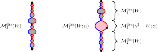
Figure 3: Suppose $0<W<\frac{\gamma^{2}}{2}$. Left: In Definition 3.5, we define the weight $W$ thin quantum disk with weight $W$ via concatenation of an ordered Poissonian collection of weight $(\gamma^{2}-W)$ thick quantum disks. Right: In Definition 3.11 we define the measure $\mathcal{M}_{2,\bullet}^{\mathrm{disk}}(W;\alpha)$ on quantum surfaces obtained by sampling three quantum surfaces from $(1-\frac{2}{\gamma^{2}}W)^{2}\mathcal{M}_{2}^{\mathrm{disk}}(W)\times\mathcal{M}_{2,\bullet}^{\mathrm{disk}}(\gamma^{2}-W;\alpha)\times\mathcal{M}_{2}^{\mathrm{disk}}(W)$ (depicted in grey, pink, grey) and concatenating them. Both: The length of the left boundary (depicted in blue) is given by the sum of the left boundary lengths of the constituent components, and the analogous statement is true for the length of the right boundary (depicted in red).

The choice of the constant $(1-\frac{2}{\gamma^{2}}W)^{-2}$ above is justified by the following proposition, which states that the quantum disk boundary length distribution extends analytically from thick to thin quantum disks, hence giving a probabilistic meaning to $\overline{R}$ and $R$ for $\beta\in(Q,Q+\frac{\gamma}{2})$.

Proposition 3.6.

For $W\in(0,\frac{\gamma^{2}}{2})$ and $\beta=\gamma+\frac{2}{\gamma}-\frac{W}{\gamma}\in(Q,Q+\frac{\gamma}{2})$, let $L_{1}$ and $L_{2}$ be the left and right boundary lengths of a thin quantum disk from $\mathcal{M}_{2}^{\mathrm{disk}}(W)$. For constants $\mu_{1},\mu_{2}\geq 0$ not both zero, the law of $\mu_{1}L_{1}+\mu_{2}L_{2}$ is

$$\mathbf{1}_{\ell>0}\overline{R}(\beta,\mu_{1},\mu_{2})\ell^{-\frac{2}{\gamma^{2}}W}\,d\ell,$$

and

$$\mathcal{M}_{2}^{\mathrm{disk}}(W)[e^{-\mu_{1}L_{1}-\mu_{2}L_{2}}]=\frac{\gamma}{2(Q-\beta)}R(\beta;\mu_{1},\mu_{2}).$$

Proof.

Note that $\mathcal{M}_{2}^{\mathrm{disk}}(W)$ is defined using Poisson point processes. Our proposition will be an immediate consequence of Campbell’s formula for the Laplace functional for Poisson point processes (see e.g.  [Kin93, Section 3.2]): For any measure space $(S,m)$ and measurable function $f:S\to(0,\infty)$ such that $\int_{S}\min(f(x),1)\,m(dx)<\infty$, we have for a Poisson point process $\Pi$ on $(S,m)$ that

$$\mathbbm{E}[\exp(-\sum_{X\in\Pi}f(X))]=\exp\mathopen{}\mathclose{{}\left(\int_{S}(e^{-f(x)}-1)\,m(dx)}\right).$$

For fixed $T>0$ we can set $S_{T}=[0,T]\times\widetilde{S}$ where $\widetilde{S}$ is the space of two-pointed quantum disks, and $m_{T}=\mathrm{Leb}_{[0,T]}\times\mathcal{M}_{2}^{\mathrm{disk}}(\gamma^{2}-W)$. Letting $\Pi_{T}$ be a Poisson point process on $(S_{T},m_{T})$ and $f(\mathcal{D})=\mu_{1}\ell_{1}+\mu_{2}\ell_{2}$ where $\ell_{1},\ell_{2}$ are the quantum lengths of the boundary arcs of $\mathcal{D}$, we have

$$\mathbbm{E}[\exp(-\sum_{(t,\mathcal{D})\in\Pi_{T}}f(\mathcal{D}))]=\exp\mathopen{}\mathclose{{}\left(-T\mathcal{M}_{2}^{\mathrm{disk}}(\gamma^{2}-W)[1-e^{-f(\mathcal{D})}]}\right).$$

Integrating against $\mathbf{1}_{T>0}(1-\frac{2}{\gamma^{2}}W)^{-2}\,dT$, we get

$$\mathcal{M}_{2}^{\mathrm{disk}}(W)[e^{-\mu_{1}L_{1}-\mu_{2}L_{2}}]=\frac{1}{(1-\frac{2}{\gamma^{2}}W)^{2}\mathcal{M}_{2}^{\mathrm{disk}}(\gamma^{2}-W)[1-e^{-f(\mathcal{D})}])}.$$

Proposition 3.4 gives $\mathcal{M}_{2}^{\mathrm{disk}}(\gamma^{2}-W)[1-e^{-f(\mathcal{D})}])=\frac{\gamma}{2(Q-\beta)}R(2Q-\beta;\mu_{1},\mu_{2})$, and combining with the reflection identity (3.8) and $1-\frac{2W}{\gamma^{2}}=\frac{2(\beta-Q)}{\gamma}$ yields the second claim.

The first assertion then follows from the fact that $\mu_{1}L_{1}+\mu_{2}L_{2}$ has a power law with exponent $-\frac{2}{\gamma^{2}}W$ [AHS20, Lemma 2.17], and a similar computation as in Proposition 3.4 to derive the coefficient of the power law. ∎

3.3 Quantum disk with a third marked boundary point

We consider the following variant of $R$ and $\overline{R}$ which has an additional parameter $\alpha$.

$$\overline{H}^{(\beta,\beta,\alpha)}_{(0,1,0)} =\mathopen{}\mathclose{{}\left(\frac{2\pi}{(\frac{\gamma}{2})^{\frac{\gamma^{2}}{4}}\Gamma(1-\frac{\gamma^{2}}{4})}}\right)^{\frac{2}{\gamma}(Q-\beta-\frac{1}{2}\alpha)}\frac{\Gamma_{\frac{\gamma}{2}}(\frac{1}{2}\alpha)^{2}\Gamma_{\frac{\gamma}{2}}(Q-\beta+\frac{1}{2}\alpha)\Gamma_{\frac{\gamma}{2}}(\beta+\frac{1}{2}\alpha-\frac{\gamma}{2})}{\Gamma_{\frac{\gamma}{2}}(\frac{2}{\gamma})\Gamma_{\frac{\gamma}{2}}(Q-\beta)^{2}\Gamma_{\frac{\gamma}{2}}(\alpha)},$$

$$H^{(\beta,\beta,\alpha)}_{(0,1,0)} =\frac{2}{\gamma}\Gamma(\frac{2}{\gamma}(\frac{1}{2}\alpha+\beta-Q))\overline{H}^{(\beta,\beta,\alpha)}_{(0,1,0)}.$$

The notations $\overline{H}^{(\beta,\beta,\alpha)}_{(0,1,0)}$ and $H^{(\beta,\beta,\alpha)}_{(0,1,0)}$ are inherited from [RZ20b] where more general more parameters are considered. The following proposition is proved in [RZ20a].

Proposition 3.7.

Suppose $\alpha>0,\frac{\alpha}{2}+\beta>\frac{\gamma}{2}$, and $\beta<Q$. Let $\widetilde{\psi}=h+(\alpha-2Q)\log|\cdot|_{+}+\frac{\beta}{2}G_{\mathbbm{H}}(\cdot,0)+\frac{\beta}{2}G_{\mathbbm{H}}(\cdot,1)$, with $h$ sampled from $P_{\mathbbm{H}}$. Then

$$\mathbbm{E}\mathopen{}\mathclose{{}\left[\nu_{\widetilde{\psi}}((0,1))^{\frac{2}{\gamma}(Q-\beta-\frac{1}{2}\alpha)}}\right]=\overline{H}^{(\beta,\beta,\alpha)}_{(0,1,0)}.$$

Proof.

The restriction of $\widetilde{\psi}$ to $(0,1)$ agrees with that of $h-\beta\log\mathopen{}\mathclose{{}\left|\cdot}\right|-\beta\log\mathopen{}\mathclose{{}\left|\cdot-1}\right|$, so $\nu_{\widetilde{\psi}}(dx)|_{[0,1]}=x^{-\frac{\gamma}{2}\beta}(1-x)^{-\frac{\gamma}{2}\beta}\mu_{h}(dx)|_{[0,1]}$. Thus the moment we consider agrees with $M(\gamma,p,a,b)$ of [RZ20a] with $a=b=-\frac{\gamma}{2}\beta$ and $p=\frac{2}{\gamma}(Q-\beta-\frac{1}{2}\alpha)$, and [RZ20a, Theorem 1.1] shows this quantity equals $\overline{H}^{(\beta,\beta,\alpha)}_{(0,1,0)}$. ∎

Recall $\mathcal{M}_{2,\bullet}^{\mathrm{disk}}(W)$ from Definition 2.17. We now extend $\mathcal{M}_{2,\bullet}^{\mathrm{disk}}(W)$ when $W>\frac{\gamma^{2}}{2}$ to have a third marked point with general $\alpha$ insertion.

Definition 3.8.

For $W>\frac{\gamma^{2}}{2}$ and $\alpha\in\mathbbm{R}$, let $\mathcal{M}_{2,\bullet}^{\mathrm{disk}}(W;\alpha)$ be the law on quantum surfaces $(\mathcal{S},\phi,-\infty,+\infty,0)$ with $\phi$ sampled from $\frac{\gamma}{2}(Q-\beta)^{-2}\mathrm{LF}_{\mathcal{S}}^{(\beta,-\infty),(\beta,+\infty),(\alpha,0)}$. We call the boundary arc between the two $\beta$ singularities which contains (resp. does not contain) the $\alpha$ singularity the marked (resp. unmarked) boundary arc.

By Proposition 2.18 we have $\mathcal{M}_{2,\bullet}^{\mathrm{disk}}(W;\gamma)=\mathcal{M}_{2,\bullet}^{\mathrm{disk}}(W)$. The next proposition describes the law of the unmarked boundary arc of $\mathcal{M}_{2,\bullet}^{\mathrm{disk}}(W;\alpha)$ for some range of $\alpha,\beta$.

Proposition 3.9.

Suppose $\alpha>0,\frac{\alpha}{2}+\beta>\frac{\gamma}{2}$, and $\beta<Q$ are as in Proposition 3.7. When a quantum disk is sampled from $\mathcal{M}_{2,\bullet}^{\mathrm{disk}}(W;\alpha)$, the law of its unmarked boundary length is

$$\mathbf{1}_{\ell>0}(Q-\beta)^{-2}\overline{H}^{(\beta,\beta,\alpha)}_{(0,1,0)}\ell^{\frac{2}{\gamma}(\beta+\frac{1}{2}\alpha-Q)-1}\,d\ell.$$ (3.9)

Proof.

By Lemma 2.11 we have $\mathrm{LF}_{\mathbbm{H}}^{(\beta,\infty),(\beta,0),(\alpha,1)}=\exp_{*}\mathrm{LF}_{\mathcal{S}}^{(\beta,\pm\infty),(\alpha,0)}$, and by Lemma 2.11 and Proposition 2.7 we have $\mathrm{LF}_{\mathbbm{H}}^{(\alpha,\infty),(\beta,0),(\beta,1)}=f_{*}\mathrm{LF}_{\mathbbm{H}}^{(\beta,\infty),(\beta,0),(\alpha,1)}$ where $f\in\mathrm{Conf}(\mathbbm{H})$ is the conformal map with $f(0)=1,f(1)=\infty,f(\infty)=0$. Therefore, the law of $\nu_{\phi}(\mathbbm{R}+\pi i)$ with $\phi$ sampled from $\mathrm{LF}_{\mathcal{S}}^{(\beta,\pm\infty),(\alpha,0)}$ agrees with the law of $\nu_{\psi}((0,1))$ with $\psi$ sampled from $\mathrm{LF}_{\mathbbm{H}}^{(\alpha,\infty),(\beta,0),(\beta,1)}$. Proposition 3.7 and the argument of Lemma 3.3 show that $\nu_{\psi}((0,1))$ has law given by $\mathbf{1}_{\ell>0}\frac{2}{\gamma}\overline{H}^{(\beta,\beta,\alpha)}_{(0,1,0)}\ell^{\frac{2}{\gamma}(\beta+\frac{1}{2}\alpha-Q)-1}\,d\ell$, so recalling the factor $\frac{\gamma}{2}(Q-\beta)^{-2}$ in the definition of $\mathcal{M}_{2,\bullet}^{\mathrm{disk}}(W;\alpha)$, we obtain the stated result. ∎

We note that if $\alpha\geq Q$, then the quantum length of the marked boundary arc is a.s. infinite because the field blows up sufficiently quickly near the marked point. Nevertheless, the unmarked boundary arc a.s. has finite quantum length as shown in Proposition 3.9.

The functions $R$ and $H$ are closely related as shown in [RZ20b, Lemma 3.4]. As a corollary of that relation we have

$$H^{(\beta,\beta,\alpha)}_{(0,1,0)}=R(\beta,1,0)^{2}H^{(2Q-\beta,2Q-\beta,\alpha)}_{(0,1,0)}\quad\text{for all }\alpha,\beta\in\mathbbm{R}.$$ (3.10)

We now give probabilistic meaning to (3.10) for some range of $\alpha$ and $\beta$.

We first recall a fact from [AHS20] which will help us define a variant of the thin quantum disk with an additional $\alpha$-insertion.

Lemma 3.10 ([AHS20, Proposition 4.4]).

For $W\in(0,\frac{\gamma^{2}}{2})$ we have

$$\mathcal{M}_{2,\bullet}^{\mathrm{disk}}(W)=(1-\frac{2}{\gamma^{2}}W)^{2}\mathcal{M}_{2}^{\mathrm{disk}}(W)\times\mathcal{M}_{2,\bullet}^{\mathrm{disk}}(\gamma^{2}-W)\times\mathcal{M}_{2}^{\mathrm{disk}}(W),$$

where the right hand side is the infinite measure on ordered collection of quantum surfaces obtained by concatenating samples from the three measures.

Definition 3.11.

Suppose $W\in(0,\frac{\gamma^{2}}{2})$ and $\alpha\in\mathbbm{R}$. Given a sample $(S_{1},S_{2},S_{3})$ from

$$(1-\frac{2}{\gamma^{2}}W)^{2}\mathcal{M}_{2}^{\mathrm{disk}}(W)\times\mathcal{M}_{2,\bullet}^{\mathrm{disk}}(\gamma^{2}-W;\alpha)\times\mathcal{M}_{2}^{\mathrm{disk}}(W),$$

let $S$ be their concatenation in the sense of Lemma 3.10 with $\alpha$ in place of $\gamma$. We define the infinite measure $\mathcal{M}_{2,\bullet}^{\mathrm{disk}}(W;\alpha)$ to be the law of $S$. Let $L$ be the sum of the left boundary lengths of $S_{1}$ and $S_{3}$, and the unmarked boundary length of $S_{2}$. We call $L$ the unmarked boundary length of $S$.

See Figure 3 for an illustration of Definition 3.11. The measure $\mathcal{M}_{2,\bullet}^{\mathrm{disk}}(W;\alpha)$ does not naturally arise in either the quantum surface or the LCFT perspective, but is quite natural in our context. The next proposition says that $\overline{H}^{(\beta,\beta,\alpha)}_{(0,1,0)}$ describes the law of its unmarked boundary length and gives a probabilistic realization of (3.10).

Proposition 3.12.

For $W\in(0,\frac{\gamma^{2}}{2})$, let $\beta=\gamma+\frac{2}{\gamma}-\frac{W}{\gamma}\in(Q,Q+\frac{\gamma}{2})$. Suppose $\alpha>2(\beta-Q)$. Then the law of the unmarked boundary length $L$ of a sample from $\mathcal{M}_{2,\bullet}^{\mathrm{disk}}(W;\alpha)$ is

$$\mathbf{1}_{\ell>0}(Q-\beta)^{-2}\overline{H}^{(\beta,\beta,\alpha)}_{(0,1,0)}\ell^{\frac{2}{\gamma}(\beta+\frac{1}{2}\alpha-Q)-1}\,d\ell.$$ (3.11)

Moreover, for $\mu>0$, we have

$$\mathcal{M}_{2,\bullet}^{\mathrm{disk}}(W;\alpha)[e^{-\mu L}]=\frac{\gamma}{2}(Q-\beta)^{-2}H^{(\beta,\beta,\alpha)}_{(0,1,0)}\mu^{-\frac{2}{\gamma}(\beta+\frac{1}{2}\alpha-Q)}$$ (3.12)

Proof.

By Proposition 3.9 the law of the unmarked boundary length $L^{\prime}$ of a sample from $\mathcal{M}_{2,\bullet}^{\mathrm{disk}}(\gamma^{2}-W;\alpha)$ is $\frac{2}{\gamma}\overline{H}^{(2Q-\beta,2Q-\beta,\alpha)}_{(0,1,0)}\ell^{b-1}\,d\ell$ with $b=\frac{2}{\gamma}(\frac{1}{2}\alpha+Q-\beta)>0$. Therefore for $\mu>0$ we have

$$\mathcal{M}_{2,\bullet}^{\mathrm{disk}}(\gamma^{2}-W;\alpha)[e^{-\mu L^{\prime}}]$$

$$\qquad=(Q-\beta)^{-2}\overline{H}^{(2Q-\beta,2Q-\beta,\alpha)}_{(0,1,0)}\Gamma(\frac{2}{\gamma}(\frac{1}{2}\alpha+Q-\beta))\mu^{\frac{2}{\gamma}(\frac{1}{2}\alpha+Q-\beta)}$$

$$\qquad=\frac{\gamma}{2}(Q-\beta)^{-2}H^{(2Q-\beta,2Q-\beta,\alpha)}_{(0,1,0)}\mu^{\frac{2}{\gamma}(\beta-Q-\frac{1}{2}\alpha)}.$$

Now by Definition 3.11, for $\mu>0$ we have

$$\begin{split}\mathcal{M}_{2,\bullet}^{\mathrm{disk}}(W;\alpha)[e^{-\mu L}]=&\,(1-\frac{2}{\gamma^{2}}W)^{2}\mathcal{M}_{2}^{\mathrm{disk}}(W)[e^{-\mu L_{2}}]\\ &\times\mathcal{M}_{2,\bullet}^{\mathrm{disk}}(\gamma^{2}-W;\alpha)[e^{-\mu L^{\prime}}]\times\mathcal{M}_{2}^{\mathrm{disk}}(W)[e^{-\mu L_{2}}],\end{split}$$

where $L_{2}$ in $\mathcal{M}_{2}^{\mathrm{disk}}(W)[e^{-\mu L_{2}}]$ means the right boundary length of a sample from $\mathcal{M}_{2}^{\mathrm{disk}}(W)$. By Proposition 3.6, we have

$$\mathcal{M}_{2}^{\mathrm{disk}}(W)[e^{-\mu L_{2}}]=\frac{\gamma}{2(Q-\beta)}R(\beta;0,\mu)=\frac{\gamma}{2(Q-\beta)}R(\beta;0,1)\mu^{\frac{2}{\gamma}(Q-\beta)}.$$

Using (3.10) we get (3.12), which further implies (3.11). ∎

4 SLE observables via conformal welding

In this section, we prove Proposition 4.5, which is a conformal welding result. Although the measures involved are infinite, a constant of proportionality that arises is finite and encodes the information of the SLE observable in Theorem 1.1.

4.1 Conformal welding of quantum disks

In this section we recall the main result from our companion paper [AHS20], saying that $\operatorname{SLE}_{\kappa}(\rho_{-};\rho_{+})$ arise as the interface between two quantum disks conformally welded together.

We start by extending the definition of a quantum surface to the case where the surface is decorated by a curve. Recall from Section 2.1 that a $\gamma$-LQG surface with $n$ marked points is defined to be an equivalence class of tuples $(D,h,z_{1},\dots,z_{n})$ where $D\subset\mathbbm{C}$ is a domain, $h$ is a distribution on $D$, and $z_{j}\in\partial D\cup D$ for $j=1,\dots,n$. A curve-decorated quantum surface with $n$ marked points is similarly defined to be an equivalence class of tuples $(D,h,z_{1},\dots,z_{n},\eta)$ where $\eta:[0,t_{\eta}]\to D$ is a curve on $D$ and $t_{\eta}$ is the duration of $\eta$. More precisely, we say that $(D,h,z_{1},\dots,z_{n},\eta)\sim_{\gamma}(\widetilde{D},\widetilde{h},\widetilde{z}_{1},\dots,\widetilde{z}_{n},\widetilde{\eta})$ if there is a conformal map $f:D\to\widetilde{D}$ such that $\widetilde{h}=f\bullet_{\gamma}h$, $\widetilde{z}_{j}=f(z_{j})$ for $j=1,\dots,n$, and $\widetilde{\eta}(t)=f(\eta(t))$.

For $W>0$, let $\mathcal{M}_{2}^{\mathrm{disk}}(W;\ell,r)$ be the measure on weight $W$ quantum disks restricting to the event that the left and right boundary arcs have lengths $\ell$ and $r$, respectively. More precisely,

$$\mathcal{M}_{2}^{\mathrm{disk}}(W)=\iint_{0}^{\infty}\mathcal{M}_{2}^{\mathrm{disk}}(W;\ell,r)\,d\ell\,dr.$$ (4.1)

In particular, $|\mathcal{M}_{2}^{\mathrm{disk}}(W;\ell,r)|d\ell\,dr$ is the law of the left and right boundary lengths, and the normalized probability measure $\mathcal{M}_{2}^{\mathrm{disk}}(W;\ell,r)^{\#}$ is $\mathcal{M}_{2}^{\mathrm{disk}}(W)$ conditioned on the boundary lengths being $\ell,r$. The identity (4.1) a priori only specifies $\mathcal{M}_{2}^{\mathrm{disk}}(W;\ell,r)$ for almost every $\ell,r$. But a canonical version of $\{\mathcal{M}_{2}^{\mathrm{disk}}(W;\ell,r):\ell,r>0\}$ can be chosen such that it is continuous in $\ell,r$ in a proper topology. See [AHS20, Section 2.6] for details.

For fixed $\ell,r,x$, a pair of quantum disks from $\mathcal{M}_{2}^{\mathrm{disk}}(W_{1};\ell,x)\times\mathcal{M}_{2}^{\mathrm{disk}}(W_{2};x,r)$ can a.s. be conformally welded along their length $x$ boundary arcs according to quantum length, yielding a quantum surface with two boundary marked points joined by an interface. This follows from the local absolute continuity of weight $W$ quantum disks with respect to weight $W$ quantum wedges, and the conformal welding theorem for quantum wedges [DMS14, Theorem 1.2]. See e.g. [She16a], [DMS14, Section 3.5], or [GHS19, Section 4.1] for more information on conformal welding in the setting of LQG surfaces.

For $W_{1},W_{2}>0$, we now define an infinite measure $\mathcal{M}_{2}^{\mathrm{disk}}(W_{1}+W_{2};\ell,r)\otimes\operatorname{SLE}_{\kappa}(W_{1}-2;W_{2}-2)$ on curve-decorated quantum surfaces. When $W_{1}+W_{2}\geq\frac{\gamma^{2}}{2}$, we first sample $\phi$ such that the law of the $(\mathcal{S},\phi,-\infty,+\infty)$ viewed as a quantum surface is $\mathcal{M}_{2}^{\mathrm{disk}}(W_{1}+W_{2};\ell,r)$ and then independently sampling an independent $\operatorname{SLE}_{\kappa}(W_{1}-2;W_{2}-2)$ curve $\eta$ in $(\mathcal{S},-\infty,+\infty)$ and parametrize $\eta$ by its quantum length. We denote the law of the curve-decorated surface $(\mathcal{S},\phi,\eta,-\infty,+\infty)$ by $\mathcal{M}_{2}^{\mathrm{disk}}(W_{1}+W_{2};\ell,r)\otimes\operatorname{SLE}_{\kappa}(W_{1}-2;W_{2}-2)$. When $W_{1}+W_{2}<\frac{\gamma^{2}}{2}$, we first sample a quantum surface with the topology of a chain of beads from $\mathcal{M}_{2}^{\mathrm{disk}}(W_{1}+W_{2};\ell,r)$, then decorate each bead by an independent $\operatorname{SLE}_{\kappa}(W_{1}-2;W_{2}-2)$ between the two marked points of the bead. We denote the law of this chain of curve-decorated surfaces $\mathcal{M}_{2}^{\mathrm{disk}}(W_{1}+W_{2};\ell,r)\otimes\operatorname{SLE}_{\kappa}(W_{1}-2;W_{2}-2)$.

The next result shows that the conformal welding of two quantum disks gives the type of curve-decorated surface defined above. For $W_{-},W_{+}>0$ and $\ell,x,r>0$, we write

$$\mathrm{Weld}(\mathcal{M}_{2}^{\mathrm{disk}}(W_{-};\ell,x),\mathcal{M}_{2}^{\mathrm{disk}}(W_{+};x,r))$$

for the measure on curve-decorated quantum surfaces obtained by first sampling $(\mathcal{D}_{-},\mathcal{D}_{+})$ from $\mathcal{M}_{2}^{\mathrm{disk}}(W_{-};\ell,x)\times\mathcal{M}_{2}^{\mathrm{disk}}(W_{+};x,r)$ and then conformally welding $\mathcal{D}_{-},\mathcal{D}_{+}$ along their length $x$ boundary arcs. This conformal welding is a.e. well defined; see [AHS20, Theorem 2.2] for details.

Proposition 4.1 ([AHS20, Theorem 2.2]).

Suppose $W_{-},W_{+}>0$. There exists a constant $c_{W_{-},W_{+}}\in(0,\infty)$ such that for all $\ell,r>0$ the following identity holds as measures on the space of curve-decorated quantum surfaces:

$$\begin{split}&\mathcal{M}_{2}^{\mathrm{disk}}(W_{-}+W_{+};\ell,r)\otimes\operatorname{SLE}_{\kappa}(W_{-}-2;W_{+}-2)\\ &\qquad\qquad=c_{W_{-},W_{+}}\int_{0}^{\infty}\mathrm{Weld}\mathopen{}\mathclose{{}\left(\mathcal{M}_{2}^{\mathrm{disk}}(W_{-};\ell,x),\mathcal{M}_{2}^{\mathrm{disk}}(W_{+};x,r)}\right)\,dx.\end{split}$$

4.2 Conformal welding of $\mathcal{M}_{2}^{\mathrm{disk}}$ and $\mathcal{M}_{2,\bullet}^{\mathrm{disk}}$

For $W>0$ with $W\neq\frac{\gamma^{2}}{2}$, let $\mathcal{M}_{2}^{\mathrm{disk}}(W;\ell):=\int_{0}^{\infty}\mathcal{M}_{2}^{\mathrm{disk}}(W;\ell,r)\,dr$. Then $\{\mathcal{M}_{2}^{\mathrm{disk}}(W;\ell)\}_{\ell>0}$ is the disintegration of $\mathcal{M}_{2}^{\mathrm{disk}}(W)$ over its left boundary length. Namely samples from $\mathcal{M}_{2}^{\mathrm{disk}}(W;\ell)$ have left boundary length $\ell$ and $\mathcal{M}_{2}^{\mathrm{disk}}(W)=\int_{0}^{\infty}\mathcal{M}_{2}^{\mathrm{disk}}(W;\ell)\,d\ell$. Recall $\mathcal{M}_{2,\bullet}^{\mathrm{disk}}(W;\alpha)$ from Definitions 3.8 and 3.11, where we insert a third boundary marked point. We now gives a concrete description of its disintegration over the unmarked boundary arc length. We start from the thick disk case $W>\frac{\gamma^{2}}{2}$.

Lemma 4.2.

For $W>\frac{\gamma^{2}}{2}$, $\beta=Q+\frac{\gamma}{2}-\frac{W}{\gamma}$, and $\alpha>\max(0,\gamma-2\beta)$, sample $h$ from $P_{\mathcal{S}}$ (the GFF on $\mathcal{S}$). Let $\widetilde{h}=h-(Q-\beta)\mathopen{}\mathclose{{}\left|\operatorname{Re}\cdot}\right|+\frac{\alpha}{2}G_{\mathcal{S}}(\cdot,0)$ and $L=\nu_{\widetilde{h}}(\mathbbm{R}+\pi i)$. For $\ell>0$, let $\mathrm{LF}_{\mathcal{S},\ell}^{(\beta,\pm\infty),(\alpha,0)}$ be the law of $\widetilde{h}+\frac{2}{\gamma}\log\frac{\ell}{L}$ under the reweighted measure $\frac{2}{\gamma}\frac{\ell^{\frac{2}{\gamma}(\beta+\frac{\alpha}{2}-Q)-1}}{L^{\frac{2}{\gamma}(\beta+\frac{\alpha}{2}-Q)}}P_{\mathcal{S}}(dh)$. Let $\mathcal{M}_{2,\bullet}^{\mathrm{disk}}(W;\alpha;\ell)$ be law of the marked quantum surface $(\mathcal{S},\phi,-\infty,+\infty,0)$ where $\phi$ is sampled from $\frac{\gamma}{2}(Q-\beta)^{-2}\mathrm{LF}_{\mathcal{S},\ell}^{(\beta,\pm\infty),(\alpha,0)}$. Then samples from $\mathcal{M}_{2,\bullet}^{\mathrm{disk}}(W;\alpha;\ell)$ have unmarked boundary arc length $\ell$ and

$$\begin{split}&\mathcal{M}_{2,\bullet}^{\mathrm{disk}}(W;\alpha)=\int_{0}^{\infty}\mathcal{M}_{2,\bullet}^{\mathrm{disk}}(W;\alpha;\ell)\,d\ell\qquad\textrm{and}\,\,\\ &|\mathcal{M}_{2,\bullet}^{\mathrm{disk}}(W;\alpha;\ell)|=(Q-\beta)^{-2}\overline{H}^{(\beta,\beta,\alpha)}_{(0,1,0)}\ell^{\frac{2}{\gamma}(\beta+\frac{1}{2}\alpha-Q)-1}.\end{split}$$ (4.2)

Proof.

The first assertion is clear since $\nu_{\widetilde{h}+\frac{2}{\gamma}\log\frac{\ell}{L}}(\mathbbm{R}+\pi i)=\frac{\ell}{L}\nu_{\widetilde{h}}(\mathbbm{R}+\pi i)=\ell$. We now prove that

$$\mathrm{LF}_{\mathcal{S}}^{(\beta,\pm\infty),(\alpha,0)}=\int_{0}^{\infty}\mathrm{LF}_{\mathcal{S},\ell}^{(\beta,\pm\infty),(\alpha,0)}\,d\ell.$$ (4.3)

For any nonnegative measurable function $F$ on $H^{-1}(\mathcal{S})$ we have

$$\begin{split}&\int_{0}^{\infty}\int F(\widetilde{h}+\frac{2}{\gamma}\log\frac{\ell}{L})\frac{2}{\gamma}\frac{\ell^{\frac{2}{\gamma}(\beta+\frac{\alpha}{2}-Q)-1}}{L^{\frac{2}{\gamma}(\beta+\frac{\alpha}{2}-Q)}}\,P_{\mathcal{S}}(dh)\,d\ell\\ &\qquad\qquad\qquad\qquad=\int\int_{\mathbbm{R}}F(\widetilde{h}+c)e^{(\beta+\frac{\alpha}{2}-Q)c}\,dc\,P_{\mathcal{S}}(dh)\end{split}$$

using Fubini’s theorem and the change of variables $c=\frac{2}{\gamma}\log\frac{\ell}{L}$. Therefore (4.3) holds. By Definition 3.8 of $\mathcal{M}_{2,\bullet}^{\mathrm{disk}}(W;\alpha)$, we have $\mathcal{M}_{2,\bullet}^{\mathrm{disk}}(W;\alpha)=\int_{0}^{\infty}\mathcal{M}_{2,\bullet}^{\mathrm{disk}}(W;\alpha;\ell)\,d\ell$. The second identify in (4.2) then directly follows from Proposition 3.9. ∎

If $W\in(0,\frac{\gamma^{2}}{2})$, $\beta=Q+\frac{\gamma}{2}-\frac{W}{\gamma}$, $\alpha>0$ and $\frac{1}{2}\alpha>\beta-Q$, then for each $\ell>0$ we can similarly define the corresponding measure $\mathcal{M}_{2,\bullet}^{\mathrm{disk}}(W;\alpha;\ell)$ on quantum surfaces with unmarked boundary arc length $\ell$ via

$$\begin{split}&\mathcal{M}_{2,\bullet}^{\mathrm{disk}}(W;\alpha;\ell):=(1-\frac{2}{\gamma^{2}}W)^{2}\int_{0}^{\ell}\int_{0}^{\ell-x}\mathcal{M}_{2}^{\mathrm{disk}}(W;x)\times\mathcal{M}_{2,\bullet}^{\mathrm{disk}}(\gamma^{2}-W;\alpha;y)\\ &\qquad\qquad\qquad\qquad\qquad\qquad\qquad\qquad\qquad\times\mathcal{M}_{2}^{\mathrm{disk}}(W;\ell-x-y)\,dy\,dx\end{split}$$ (4.4)

where the integrand is understood as concatenation of surfaces in the sense of Lemma 3.10.

Lemma 4.3.

For $W\in(0,\frac{\gamma^{2}}{2})$, (4.2) still holds with the $\mathcal{M}_{2,\bullet}^{\mathrm{disk}}(W;\alpha;\ell)$ defined above.

Proof.

The first claim is immediate from Definition 3.11, and the second then follows from Proposition 3.12. ∎

Recall that the special case of $\mathcal{M}_{2,\bullet}^{\mathrm{disk}}(W;\alpha)$ with $\alpha=\gamma$ is $\mathcal{M}_{2,\bullet}^{\mathrm{disk}}(W)$ from Definition 2.17. We now give a variant of Proposition 4.1 for $\mathcal{M}_{2,\bullet}^{\mathrm{disk}}(W;\gamma)$. The $\mathrm{Weld}$ notation in our next two results is used analogously as in Proposition 4.1.

Lemma 4.4.

For $W_{-},W_{+}>0$ with $W_{+},W_{-}+W_{+}\neq\frac{\gamma^{2}}{2}$, there is a constant $c_{W_{-},W_{+}}\in(0,\infty)$ such that for each $\ell>0$

$$\begin{split}&\mathcal{M}_{2,\bullet}^{\mathrm{disk}}(W_{-}+W_{+};\gamma;\ell)\otimes\operatorname{SLE}_{\kappa}(W_{-}-2;W_{+}-2)\\ &=c_{W_{-},W_{+}}\int_{0}^{\infty}\mathrm{Weld}\mathopen{}\mathclose{{}\left(\mathcal{M}_{2}^{\mathrm{disk}}(W_{-};\ell,x),\mathcal{M}_{2,\bullet}^{\mathrm{disk}}(W_{+};\gamma;x)}\right)\,dx.\end{split}$$ (4.5)

Proof.

In Proposition 4.1, sample a marked point from quantum length measure on the boundary arc of length $r$ (thus weighting by $r$). The result then follows from Proposition 2.18 or Lemma 3.10, depending on whether the quantum disks are thick or thin. ∎

We now extend Lemma 4.4 to $\mathcal{M}_{2,\bullet}^{\mathrm{disk}}(W;\alpha)$; see Figure 4 for an illustration. We first introduction an $\alpha$ variant of $\operatorname{SLE}_{\kappa}(W_{-}-2;W_{+}-2)$. Given a curve $\eta$ on $\mathcal{S}$ from $-\infty$ to $\infty$, let $D$ be the connected component of $\mathcal{S}\backslash\eta$ containing $0$ on its boundary, and let $\psi_{\eta}:D\to\mathcal{S}$ be the conformal map fixing $0$ and sending the first (resp. last) point on $\partial D$ hit by $\eta$ to $-\infty$ (resp. $+\infty$). For $\alpha\in\mathbbm{R}$, let $\Delta(\alpha)=\frac{\alpha}{2}(Q-\frac{\alpha}{2})$. For $W_{-},W_{+}>0$, we define the measure $\mathsf{m}(W_{-},W_{+},\alpha)$ on curves on $\mathcal{S}$ such that its Radon-Nikodym derivative with respect to $\operatorname{SLE}_{\kappa}(W_{-}-2;W_{+}-2)$ is:

$$\frac{d\mathsf{m}(W_{-},W_{+},\alpha)}{d\operatorname{SLE}_{\kappa}(W_{-}-2;W_{+}-2)}(\eta)=\psi_{\eta}^{\prime}(0)^{1-\Delta(\alpha)}.$$

When $W_{-}+W_{+}\geq\frac{\gamma^{2}}{2}$, we define $\mathcal{M}_{2,\bullet}^{\mathrm{disk}}(W_{-}+W_{+};\alpha;\ell)\otimes\mathsf{m}(W_{-},W_{+},\alpha)$ in the exact same way as $\mathcal{M}_{2,\bullet}^{\mathrm{disk}}(W_{-}+W_{+};\gamma;\ell)\otimes\operatorname{SLE}_{\kappa}(W_{-}-2;W_{+}-2)$ in Lemma 4.4 with $\mathsf{m}(W_{-},W_{+},\alpha)$ in place of $\operatorname{SLE}_{\kappa}(W_{-}-2;W_{+}-2)$. When $W_{-}+W_{+}<\frac{\gamma^{2}}{2}$, we still define $\mathcal{M}_{2,\bullet}^{\mathrm{disk}}(W_{-}+W_{+};\alpha;\ell)\otimes\mathsf{m}(W_{-},W_{+},\alpha)$ as a chain of curve-decorated quantum surfaces as $\mathcal{M}_{2,\bullet}^{\mathrm{disk}}(W_{-}+W_{+};\gamma;\ell)\otimes\operatorname{SLE}_{\kappa}(W_{-}-2;W_{+}-2)$, except that for the quantum surface containing the additional boundary marked point, we use $\mathsf{m}(W_{-},W_{+},\alpha)$ instead of $\operatorname{SLE}_{\kappa}(W_{-}-2;W_{+}-2)$ to decorate that surface.

Proposition 4.5.

For $W_{-}\geq\frac{\gamma^{2}}{2}$ and $W_{+}>0$ with $W_{+}\neq\frac{\gamma^{2}}{2}$, there is a constant $c_{W_{-},W_{+}}\in(0,\infty)$ such that for all $\alpha\in\mathbbm{R}$ and $\ell>0$

$$\begin{split}&\mathcal{M}_{2,\bullet}^{\mathrm{disk}}(W_{-}+W_{+};\alpha;\ell)\otimes\mathsf{m}(W_{-},W_{+},\alpha)\\ &=c_{W_{-},W_{+}}\int_{0}^{\infty}\mathrm{Weld}\mathopen{}\mathclose{{}\left(\mathcal{M}_{2}^{\mathrm{disk}}(W_{-};\ell,x),\mathcal{M}_{2,\bullet}^{\mathrm{disk}}(W_{+};\alpha;x)}\right)\,dx.\end{split}$$ (4.6)

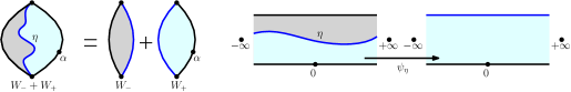
Figure 4: Proposition 4.5 when $W_{+}>\frac{\gamma^{2}}{2}$. Left: Illustration of (4.6). Right: Definition of $\psi_{\eta}$.

In the next section we will use Proposition 4.5 to compute $|\mathsf{m}(W_{-},W_{+},\alpha)|$, which equals $\mathbbm{E}[\psi^{\prime}(0)^{1-\Delta(\alpha)}]$ by definition. The key to the proof of Proposition 4.5 is the following lemma based on Girsanov theorem.

Lemma 4.6.

Let $\alpha_{1},\alpha_{2},\beta\in\mathbbm{R}$ and $\ell>0$. Then we have the weak convergence of measures

$$\lim_{\varepsilon\to 0}\varepsilon^{\frac{1}{4}(\alpha_{2}^{2}-\alpha_{1}^{2})}e^{\frac{(\alpha_{2}-\alpha_{1})}{2}\phi_{\varepsilon}(0)}\mathrm{LF}_{\mathcal{S},\ell}^{(\beta,\pm\infty),(\alpha_{1},0)}(d\phi)=\mathrm{LF}_{\mathcal{S},\ell}^{(\beta,\pm\infty),(\alpha_{2},0)},$$ (4.7)

and moreover $\mathopen{}\mathclose{{}\left|\varepsilon^{\frac{1}{4}(\alpha_{2}^{2}-\alpha_{1}^{2})}e^{\frac{(\alpha_{2}-\alpha_{1})}{2}\phi_{\varepsilon}(0)}\mathrm{LF}_{\mathcal{S},\ell}^{(\beta,\pm\infty),(\alpha_{1},0)}(d\phi)}\right|\big{/}\mathopen{}\mathclose{{}\left|\mathrm{LF}_{\mathcal{S},\ell}^{(\beta,\pm\infty),(\alpha_{2},0)}}\right|=1+o_{\varepsilon}(1)$ where the error $o_{\varepsilon}(1)$ converge to 0 uniformly in $\ell$.

Proof.

When $\phi$ is sampled from $(\mathrm{LF}_{\mathcal{S},1}^{(\beta,\pm\infty),(\alpha,0)})^{\#}$, the law of $\phi+\frac{2}{\gamma}\log\ell$ is $(\mathrm{LF}_{\mathcal{S},\ell}^{(\beta,\pm\infty),(\alpha,0)})^{\#}$. Moreover, by Lemma 4.2

$$\frac{\mathopen{}\mathclose{{}\left|e^{\frac{(\alpha_{2}-\alpha_{1})}{2}\phi_{\varepsilon}(0)}\mathrm{LF}_{\mathcal{S},\ell}^{(\beta,\pm\infty),(\alpha_{1},0)}(d\phi)}\right|}{\mathopen{}\mathclose{{}\left|e^{\frac{(\alpha_{2}-\alpha_{1})}{2}\phi_{\varepsilon}(0)}\mathrm{LF}_{\mathcal{S},1}^{(\beta,\pm\infty),(\alpha_{1},0)}(d\phi)}\right|}=\frac{\mathopen{}\mathclose{{}\left|\mathrm{LF}_{\mathcal{S},\ell}^{(\beta,\pm\infty),(\alpha_{2},0)}}\right|}{\mathopen{}\mathclose{{}\left|\mathrm{LF}_{\mathcal{S},1}^{(\beta,\pm\infty),(\alpha_{2},0)}}\right|}=\ell^{\frac{2}{\gamma}(\beta+\frac{\alpha_{2}}{2}-Q)-1.}$$

Therefore, it suffices to prove (4.7) for $\ell=1$. To this end, for $\varepsilon>0$, let $G_{\mathcal{S},\varepsilon}(z,0):=\mathbbm{E}[h(z)h_{\varepsilon}(0)]$. For a distribution $h$, let $\widetilde{h}^{j}:=h-(Q-\beta)\mathopen{}\mathclose{{}\left|\operatorname{Re}\cdot}\right|+\frac{\alpha_{j}}{2}G_{\mathcal{S}}(\cdot,0)$ for $j=1,2$, and let $\widetilde{h}^{2,\varepsilon}:=\widetilde{h}^{1}+\frac{\alpha_{2}-\alpha_{1}}{2}G_{\mathcal{S},\varepsilon}$. Let $f$ be a bounded and continuous functional on $H^{-1}(\mathcal{S})$ (see Remark 2.3). Then

$$\int\varepsilon^{\frac{1}{4}(\alpha_{2}^{2}-\alpha_{1}^{2})}e^{\frac{(\alpha_{2}-\alpha_{1})}{2}(\widetilde{h}^{1}_{\varepsilon}(0)-\frac{2}{\gamma}\log{\nu_{\widetilde{h}^{1}}(\mathbbm{R}+\pi i)})}f(\widetilde{h}^{1}-\frac{2}{\gamma}\log{\nu_{\widetilde{h}^{1}}(\mathbbm{R}+\pi i)})$$

$$\qquad\qquad\frac{2}{\gamma}\nu_{\widetilde{h}^{1}}(\mathbbm{R}+\pi i)^{-\frac{2}{\gamma}(\beta+\frac{\alpha_{1}}{2}-Q)}P_{\mathcal{S}}(dh)$$

$$=\int(1+o_{\varepsilon}(1))\mathbbm{E}[e^{\frac{\alpha_{2}-\alpha_{1}}{2}h_{\varepsilon}(0)}]^{-1}e^{\frac{\alpha_{2}-\alpha_{1}}{2}h_{\varepsilon}(0)}f(\widetilde{h}^{1}-\frac{2}{\gamma}\log{\nu_{\widetilde{h}^{1}}(\mathbbm{R}+\pi i)})$$

$$\qquad\qquad\frac{2}{\gamma}{\nu_{\widetilde{h}^{1}}(\mathbbm{R}+\pi i)^{-\frac{2}{\gamma}(\beta+\frac{\alpha_{2}}{2}-Q)}}P_{\mathcal{S}}(dh)$$

$$=\int(1+o_{\varepsilon}(1))f(\widetilde{h}^{2,\varepsilon}-\frac{2}{\gamma}\log{\nu_{\widetilde{h}^{2,\varepsilon}}(\mathbbm{R}+\pi i)})\frac{2}{\gamma}{\nu_{\widetilde{h}^{2,\varepsilon}}(\mathbbm{R}+\pi i)^{-\frac{2}{\gamma}(\beta+\frac{\alpha_{2}}{2}-Q)}}P_{\mathcal{S}}(dh)$$

$$\stackrel{{\scriptstyle\varepsilon\to 0}}{{\longrightarrow}}\int f(\widetilde{h}^{2}-\frac{2}{\gamma}\log{\nu_{\widetilde{h}^{2}}(\mathbbm{R}+\pi i)})\frac{2}{\gamma}{\nu_{\widetilde{h}^{2}}(\mathbbm{R}+\pi i)^{-\frac{2}{\gamma}(\beta+\frac{\alpha_{2}}{2}-Q)}}P_{\mathcal{S}}(dh)$$

$$=\int f(\phi)\mathrm{LF}_{\mathcal{S},\ell}^{(\beta,\pm\infty),(\alpha_{2},0)}(d\phi).$$

In the first equality, we are using that the average of $-(Q-\beta)\mathopen{}\mathclose{{}\left|\operatorname{Re}\cdot}\right|+\frac{\alpha_{1}}{2}G_{\mathcal{S}}(\cdot,0)$ on $\partial B_{\varepsilon}(0)\cap\mathcal{S}$ is $-\alpha_{1}\log\varepsilon+o_{\varepsilon}(1)$, and $\mathbbm{E}[e^{\frac{\alpha_{2}-\alpha_{1}}{2}h_{\varepsilon}(0)}]=(1+o_{\varepsilon}(1))\varepsilon^{-\frac{1}{4}(\alpha_{2}-\alpha_{1})^{2}}$. The second equality uses Girsanov’s theorem, and the final limit uses the dominated convergence theorem and $\nu_{\widetilde{h}^{2}}(\mathbbm{R}+\pi i)=(1+o_{\varepsilon}(1))\nu_{\widetilde{h}^{2,\varepsilon}}(\mathbbm{R}+\pi i)$ with error $o_{\varepsilon}(1)$ uniform in $h$ (indeed $\sup_{z\in\mathbbm{R}+\pi i}|G_{\mathcal{S}}(z,0)-G_{\mathcal{S},\varepsilon}(z,0)|=o_{\varepsilon}(1)$). Since $f$ can be arbitrary we obtain (4.7) for $\ell=1$. ∎

Proof of Proposition 4.5.

We will weight (4.5) to obtain the proposition. We explain first the case $W_{+}>\frac{\gamma^{2}}{2}$, then the modifications needed for $W_{+}<\frac{\gamma^{2}}{2}$.

Consider $W_{+}>\frac{\gamma^{2}}{2}$ and let $\beta_{+}=Q+\frac{\gamma}{2}-\frac{W_{+}}{\gamma},\beta=Q+\frac{\gamma}{2}-\frac{W}{\gamma}$. Sample $(Y,\eta)$ from $\frac{\gamma}{2}(Q-\beta)^{-2}\mathrm{LF}_{\mathcal{S},\ell}^{(\beta,\pm\infty),(\gamma,0)}\times\operatorname{SLE}_{\kappa}(W_{-}-2;W_{+}-2)$, so $(\mathcal{S},Y,-\infty,+\infty,0)/{\sim_{\gamma}}$ has law given by the left hand side of (4.5). Let $\xi_{\eta}$ be the map from the connected component of $\mathcal{S}\backslash\eta$ containing the boundary arc $\mathbbm{R}\pi i$ to $\mathcal{S}$ such that $\xi_{\eta}$ fixes $\pm\infty$ and $\pi i$. Set

$$X=Y\circ\psi_{\eta}^{-1}+Q\log\mathopen{}\mathclose{{}\left|(\psi_{\eta}^{-1})^{\prime}}\right|,\quad Z=Y\circ\xi_{\eta}^{-1}+Q\log\mathopen{}\mathclose{{}\left|(\xi_{\eta}^{-1})^{\prime}}\right|.$$ (4.8)

By Lemma 4.4, the conditional law of $(\mathcal{S},Z,\pm\infty)/{\sim_{\gamma}}$ given $X$ is $\mathcal{M}_{2}^{\mathrm{disk}}(\frac{\gamma^{2}}{2};\ell,\nu_{X}(\mathbbm{R}+\pi i))^{\#}$, and the marginal law of $X$ is

$$c_{W_{-},W_{+}}\int_{0}^{\infty}\int_{0}^{\infty}\overline{R}(\beta_{1};1,0)x^{-\frac{2}{\gamma}W_{-}}\frac{\gamma}{2}(Q-\beta)^{-2}\mathrm{LF}_{\mathcal{S},x}^{(\beta_{+},-\infty),(\beta_{+},+\infty),(\gamma,0)}\,dx.$$ (4.9)

Here, the expression $\frac{\gamma}{2}(Q-\beta)^{-2}\mathrm{LF}_{\mathcal{S}}^{(\beta_{+},-\infty),(\beta_{+},+\infty),(\gamma,0)}$ comes from Proposition 2.18, and the prefactor arises from the weighting induced by welding since $|\mathcal{M}_{2}^{\mathrm{disk}}(W_{-};\ell)|=\overline{R}(\beta_{1};1,0)\ell^{-\frac{2}{\gamma}W_{-}}$.

By Lemma 4.6, if we weight the law of $(X,Z)$ by $\varepsilon^{\frac{1}{4}(\alpha^{2}-\gamma^{2})}e^{\frac{\alpha-\gamma}{2}X_{\varepsilon}(0)}$, as $\varepsilon\to 0$ the marginal law of $X$ converges to

$$c_{W_{-},W_{+}}\int_{0}^{\infty}\overline{R}(\beta_{1};1,0)x^{-\frac{2}{\gamma}W_{-}}\frac{\gamma}{2}(Q-\beta)^{-2}\mathrm{LF}_{\mathcal{S},x}^{(\beta_{+},-\infty),(\beta_{+},+\infty),(\alpha,0)}\,dx,$$ (4.10)

and moreover the conditional law of $(\mathcal{S},Z,\pm\infty)/{\sim_{\gamma}}$ given $X$ is still $\mathcal{M}_{2}^{\mathrm{disk}}(\frac{\gamma^{2}}{2};\ell,\nu_{X}(\mathbbm{R}+\pi i))^{\#}$ in the limit.

For $\varepsilon\in(0,1)$ let $\theta_{\varepsilon}$ denote the uniform probability measure on $B_{\varepsilon}(0)\cap\mathcal{S}$ such that we have $h_{\varepsilon}(0)=(h,\theta_{\varepsilon})$. Let $\theta^{\eta}_{\varepsilon}=(\psi_{\eta}^{-1})_{*}\theta_{\varepsilon}$ denote the pushforward of $\theta$ under $\psi_{\eta}^{-1}$. By Schwarz reflection we can extend $\psi_{\eta}^{-1}:\mathcal{S}\to\mathcal{S}$ to a holomorphic map $f$ from $\mathbbm{R}\times(-\pi,\pi)$ to itself. Since $f^{\prime}$ is holomorphic, $\log|f^{\prime}|$ is harmonic and hence $(\log|f^{\prime}|,\theta_{\varepsilon})=\log|f^{\prime}(0)|$ by the mean value property of harmonic functions. Thus, by (4.8)

$$X_{\varepsilon}(0)=(Y\circ\psi^{-1}+Q\log|(\psi_{\eta}^{-1})^{\prime}|,\theta_{\varepsilon})=(Y,\theta^{\eta}_{\varepsilon})+Q\log|(\psi_{\eta}^{-1})^{\prime}(0)|,$$ (4.11)

and so weighting $X$ by $\varepsilon^{\frac{1}{4}(\alpha^{2}-\gamma^{2})}e^{\frac{\alpha-\gamma}{2}X_{\varepsilon}(0)}$ corresponds to weighting $(Y,\eta)$ by

$$\varepsilon^{\frac{1}{4}(\alpha^{2}-\gamma^{2})}e^{\frac{\alpha-\gamma}{2}((Y,\theta^{\eta}_{\varepsilon})-Q\log|\psi_{\eta}^{\prime}(0)|)}=\mathopen{}\mathclose{{}\left(\frac{\varepsilon}{\psi_{\eta}^{\prime}(0)}}\right)^{\frac{1}{4}(\alpha^{2}-\gamma^{2})}e^{\frac{\alpha-\gamma}{2}(Y,\theta^{\eta}_{\varepsilon})}\cdot|\psi_{\eta}^{\prime}(0)|^{\frac{1}{4}\alpha^{2}-\frac{Q}{2}\alpha+1}.$$ (4.12)

Now we note that for any fixed curve $\eta_{0}$ in $\overline{\mathcal{S}}$ from $-\infty$ to $+\infty$ that does not hit $0$, we have a distortion estimate $|(\psi_{\eta_{0}}^{-1})^{\prime}(z)-(\psi_{\eta_{0}}^{-1})^{\prime}(0)|/|(\psi_{\eta_{0}}^{-1})^{\prime}(0)|=o_{\varepsilon}(1)$ for $|z|<\varepsilon$, with $o_{\varepsilon}(1)$ not depending on $\eta_{0}$. This follows e.g. from [Law05, Theorem 3.21], which gives the analogous bound for interior points and can be applied to $\psi_{\eta_{0}}^{-1}$ after extension by Schwarz reflection. Thus, when $h$ is sampled from $P_{\mathcal{S}}$ we have $\mathbbm{E}[e^{\frac{\alpha-\gamma}{2}(h,\theta^{\eta_{0}}_{\varepsilon})}]=(1+o_{\varepsilon}(1))\mathopen{}\mathclose{{}\left(\frac{\varepsilon}{\psi^{\prime}_{\eta_{0}}(0)}}\right)^{-(\frac{\alpha-\gamma}{2})^{2}}$, where $o_{\varepsilon}(1)$ does not depend on $\eta_{0}$. Using this fact and the argument of Lemma 4.6, we obtain Lemma 4.6 with $\varepsilon$ replaced by $\varepsilon/\psi_{\eta_{0}}^{\prime}(0)$ and $\phi_{\varepsilon}$ replaced by $(\phi,\theta_{\varepsilon}^{\eta_{0}})$, where the $o_{\varepsilon}(1)$ errors do not depend on $\eta_{0}$. Therefore, for any bounded measurable function $g$ on the space of curves in $\mathcal{S}$ from $-\infty$ to $+\infty$ equipped with the Hausdorff topology and any bounded continuous function $F:(H^{-1}(\mathcal{S}))^{3}\to\mathbbm{R}$ we have

$$\lim_{\varepsilon\to 0}\int\mathopen{}\mathclose{{}\left(\int\mathopen{}\mathclose{{}\left(\frac{\varepsilon}{\psi_{\eta}^{\prime}(0)}}\right)^{\frac{1}{4}(\alpha^{2}-\gamma^{2})}e^{\frac{\alpha-\gamma}{2}(Y,\theta^{\eta}_{\varepsilon})}F(X,Y,Z)\frac{\gamma}{2}(Q-\beta)^{-2}\mathrm{LF}_{\mathcal{S},\ell}^{(\beta,\pm\infty),(\gamma,0)}(dY)}\right)$$

$$\qquad\qquad\qquad\qquad\qquad\qquad\qquad\qquad\qquad\qquad\qquad g(\eta)\mathsf{m}(W_{-},W_{+},\alpha)(d\eta)$$

$$=\int\mathopen{}\mathclose{{}\left(\int F(\widetilde{X},\widetilde{Y},\widetilde{Z})\frac{\gamma}{2}(Q-\beta)^{-2}\mathrm{LF}_{\mathcal{S},\ell}^{(\beta,\pm\infty),(\alpha,0)}(d\widetilde{Y})}\right)g(\widetilde{\eta})\mathsf{m}(W_{-},W_{+},\alpha)(d\widetilde{\eta})$$

where $X,Z$ (resp. $\widetilde{X},\widetilde{Z}$) are the functions of $(Y,\eta)$ (resp. $(\widetilde{Y},\widetilde{\eta})$) given by (4.8). That is, as $\varepsilon\to 0$ the weighted law of $(X,Y,Z,\eta)$ converges to the law of $(\widetilde{X},\widetilde{Y},\widetilde{Z},\widetilde{\eta})$. Thus, when $(\widetilde{Y},\widetilde{\eta})$ is sampled from $\frac{\gamma}{2}(Q-\beta)^{-2}\mathrm{LF}_{\mathcal{S},\ell}^{(\beta,\pm\infty),(\alpha,0)}\times\mathsf{m}(W_{-},W_{+},\alpha)$, the law of $\widetilde{X}$ is (4.10), and the conditional law of $(\mathcal{S},\widetilde{Z},\pm\infty)$ given $\widetilde{X}$ is $\mathcal{M}_{2}^{\mathrm{disk}}(\frac{\gamma^{2}}{2};\ell,\nu_{X}(\mathbbm{R}+\pi i))^{\#}$. This concludes the proof in the case $W_{+}>\frac{\gamma^{2}}{2}$.

For the case $W_{+}<\frac{\gamma^{2}}{2}$, the quantum surface to the right of the curve is no longer simply connected. By Lemma 3.10, this quantum surface can be described as the concatenation of $(\mathcal{D}_{1},\mathcal{D}_{\bullet},\mathcal{D}_{2})$ sampled from

$$\overline{R}(\beta_{1};1,0)L^{-\frac{2}{\gamma}W_{-}}(1-\frac{2}{\gamma^{2}}W_{+})^{2}\mathcal{M}_{2}^{\mathrm{disk}}(W_{+})\times\mathcal{M}_{2,\bullet}^{\mathrm{disk}}(\gamma^{2}-W_{+})\times\mathcal{M}_{2}^{\mathrm{disk}}(W_{+}),$$ (4.13)

where $L$ is the sum of the left boundary lengths of $(\mathcal{D}_{1},\mathcal{D}_{\bullet},\mathcal{D}_{2})$. Parametrizing $\mathcal{D}_{\bullet}$ as $(\mathcal{S},X,-\infty,+\infty,0)$, and arguing exactly as before, we obtain the proposition. ∎

5 The shift relations and proof of Theorem 1.1

In this section we use the welding equation from Proposition 4.5 and the integrability for quantum disks from LCFT and mating-of-trees to prove Theorem 1.1 as outlined in Section 1.3. In Section 5.1, we recall the mating-of-trees theorem for the quantum disk which gives the joint law of the boundary lengths in $\mathcal{M}_{2}^{\mathrm{disk}}(2)$. Using this theorem we further derive the analogous result for $\mathcal{M}_{2}^{\mathrm{disk}}(\frac{\gamma^{2}}{2})$. In Section 5.2 we obtain Theorem 1.1 in the cases where $\beta_{-}$ corresponds to $W_{-}\in\{\frac{\gamma^{2}}{2},2\}$ and $\beta_{+}$ to generic $W_{+}$. This is based on exact results on the length distribution of quantum disks from Section 5.1 for the two special weights, and the ones from Section 3 via LCFT for generic weight. Finally, we derive shift relations in Section 5.3 and complete the proof of Theorem 1.1.

5.1 Integrability of weights $2$ and $\gamma^{2}/2$ quantum disk via mating of trees

Although Lemma 3.3 and Proposition 3.4 and their thin quantum disk counterparts uniquely characterize the total mass of $\mathcal{M}_{2}^{\mathrm{disk}}(W;\ell,r)$ in terms of the reflection coefficient $R$, it is quite complicated in general. For $W\in\{2,\gamma^{2}/2\}$, we have a much simpler description from [AHS20].

Proposition 5.1 ([AHS20, Propositions 7.7 and 7.8]).

For $\ell,r>0$ we have

$$|\mathcal{M}_{2}^{\mathrm{disk}}(2;\ell,r)|=C_{1}(\ell+r)^{-\frac{4}{\gamma^{2}}-1}\quad\textrm{and}\quad|\mathcal{M}_{2}^{\mathrm{disk}}(\frac{\gamma^{2}}{2};\ell,r)|=C_{2}\frac{(\ell r)^{4/\gamma^{2}-1}}{(\ell^{4/\gamma^{2}}+r^{4/\gamma^{2}})^{2}}.$$

We do not need the values of $C_{1}$ and $C_{2}$, but they are easy to derive using results from Section 3.

Proposition 5.2.

For $\ell,r>0$ we have

$$|\mathcal{M}_{2}^{\mathrm{disk}}(2;\ell,r)|=\frac{(2\pi)^{\frac{4}{\gamma^{2}}-1}}{(1-\frac{\gamma^{2}}{4})\Gamma(1-\frac{\gamma^{2}}{4})^{\frac{4}{\gamma^{2}}}}(\ell+r)^{-\frac{4}{\gamma^{2}}-1},$$

$$|\mathcal{M}_{2}^{\mathrm{disk}}(\frac{\gamma^{2}}{2};\ell,r)|=\frac{4}{\gamma^{2}}\frac{(\ell r)^{4/\gamma^{2}-1}}{(\ell^{4/\gamma^{2}}+r^{4/\gamma^{2}})^{2}}.$$

Proof.

By Lemma 3.3 with $W=2$ , the law of the quantum length of the left boundary arc of $\mathcal{M}_{2}^{\mathrm{disk}}(2)$ is $\mathbf{1}_{\ell>0}\overline{R}(\gamma,1,0)\ell^{-\frac{4}{\gamma^{2}}}$ with $\overline{R}(\gamma,1,0)$ as in (3.4). By Proposition 5.1, we have

$$\begin{split}\overline{R}(\gamma,1,0)=\int_{0}^{\infty}C_{1}(1+r)^{-\frac{4}{\gamma^{2}}-1}\,dr=\frac{C_{1}\gamma^{2}}{4},\end{split}$$

and applying the shift equations (3.2) to (3.4), we have

$$\begin{split}\overline{R}(\gamma,1,0)&=\frac{(2\pi)^{\frac{4}{\gamma^{2}}-\frac{3}{2}}(\frac{2}{\gamma})^{-\frac{1}{2}-\frac{\gamma^{2}}{4}}}{(1-\frac{\gamma^{2}}{4})\Gamma(1-\frac{\gamma^{2}}{4})^{\frac{4}{\gamma^{2}}-1}}\frac{\Gamma_{\frac{\gamma}{2}}(\frac{\gamma}{2})}{\Gamma_{\frac{\gamma}{2}}(Q)}\frac{\Gamma_{\frac{\gamma}{2}}(Q)}{\Gamma_{\frac{\gamma}{2}}(\frac{2}{\gamma})}\frac{\Gamma_{\frac{\gamma}{2}}(\frac{2}{\gamma})}{\Gamma_{\frac{\gamma}{2}}(\frac{2}{\gamma}-\frac{\gamma}{2})}\\ &=\frac{\gamma^{2}}{4}\frac{(2\pi)^{\frac{4}{\gamma^{2}}-1}}{(1-\frac{\gamma^{2}}{4})\Gamma(1-\frac{\gamma^{2}}{4})^{\frac{4}{\gamma^{2}}}}.\end{split}$$

This gives $C_{1}$. Similarly, by Lemma 3.3 with $W=\frac{\gamma^{2}}{2}$, the law of the quantum length of the left boundary arc of $\mathcal{M}_{2}^{\mathrm{disk}}(\frac{\gamma^{2}}{2})$ is $\mathbf{1}_{\ell>0}\ell^{-1}d\ell$. By Proposition 5.1 and using the change of variables $t=r^{4/\gamma^{2}}$, we have

$$1=\int_{0}^{\infty}C_{2}\frac{r^{4/\gamma^{2}-1}}{(1+r^{4/\gamma^{2}})^{2}}\,dr=\frac{C_{2}\gamma^{2}}{4}\int_{0}^{\infty}\frac{1}{(1+t)^{2}}=\frac{C_{2}\gamma^{2}}{4}.\qed$$

5.2 Special cases of Theorem 1.1

In this section, we leverage exact formulas for $|\mathcal{M}_{2}^{\mathrm{disk}}(2;\ell,r)|$ and $|\mathcal{M}_{2}^{\mathrm{disk}}(\frac{\gamma^{2}}{2};\ell,r)|$ to show Proposition 5.6, which is Theorem 1.1 in the cases where $\kappa\in(0,4)$ and $\rho_{-}\in\{0,\frac{\kappa}{2}\}$.

We will use the parameters from LQG and conformal welding to express the moment in Theorem 1.1. More precisely, for $\gamma\in(0,2),\lambda\in\mathbbm{R}$ and $\beta_{-},\beta_{+}<Q+\frac{\gamma}{2}$ we set

$$m^{\lambda}_{\gamma}(\beta_{-},\beta_{+}):=\mathbbm{E}[\psi^{\prime}(1)^{\lambda}]$$ (5.1)

where $\mathbbm{E}[\psi^{\prime}(1)^{\lambda}]$ is the moment in Theorem 1.1 with

$$\kappa=\gamma^{2}\in(0,4),\quad\rho_{-}=\gamma^{2}-\gamma\beta_{-}>-2,\quad\textrm{and}\quad\rho_{+}=\gamma^{2}-\gamma\beta_{+}>-2.$$ (5.2)

We first make some basic observations on $m^{\lambda}_{\gamma}(\beta_{-},\beta_{+})$.

Lemma 5.3.

If $m^{\lambda}_{\gamma}(\beta_{-},\beta_{+})<\infty$ and $\lambda<\lambda^{\prime}$ then $m^{\lambda}_{\gamma}(\beta_{-},\beta_{+})<m^{\lambda^{\prime}}_{\gamma}(\beta_{-},\beta_{+})$. Moreover, $m^{0}_{\gamma}(\beta_{-},\beta_{+})=1$.

Proof.

From the definition of $\psi$, we see that $\psi^{\prime}(1)>1$ a.s., giving the monotonicity property. The second observation is trivial. ∎

Since we can conformally map from $(\mathbbm{H},0,\infty,1)$ to $(\mathcal{S},-\infty,+\infty,0)$, from the definition of $\mathsf{m}(W_{-},W_{+},\alpha)$ above Proposition 4.5, we see that

$$|\mathsf{m}(W_{-},W_{+},\alpha)|=m^{\lambda}_{\gamma}(\beta_{-},\beta_{+})\quad\textrm{with }W_{\pm}=\gamma(\gamma+\frac{2}{\gamma}-\beta_{\pm})$$ (5.3)

Now we can compute $m^{\lambda}_{\gamma}(\beta_{-},\beta_{+})$ by computing $|\mathsf{m}(W_{-},W_{+},\alpha)|$ via Proposition 4.5. Based on this idea, the following lemma computes $m^{\lambda}_{\gamma}(\gamma,\beta_{+})$ for $\beta_{+}\neq Q$ and a certain range of $\lambda$, modulo a $\beta_{+}$-dependent multiplicative constant. The range of $\lambda$ below does not contain $0$. Later we will remove this restriction so that the constant can be recovered from $m^{0}_{\gamma}(\beta_{-},\beta_{+})=1$.

Lemma 5.4.

For any $\beta_{+}\in(-\infty,Q)\cup(Q,Q+\frac{\gamma}{2})$ and $\alpha\in(2|\beta_{+}-Q|,4Q-2\beta_{+})$, set $\lambda=1-\frac{\alpha}{2}(Q-\frac{\alpha}{2})$. Then there is a constant $C=C_{\gamma}(\beta_{+})\in(0,\infty)$ not depending on $\alpha$ such that

$$m^{\lambda}_{\gamma}(\gamma,\beta_{+})=C_{\gamma}(\beta_{+})\,\Gamma(\frac{2}{\gamma}(Q-\beta_{+}+\frac{1}{2}\alpha))\Gamma(\frac{2}{\gamma}(2Q-\beta_{+}-\frac{1}{2}\alpha)).$$ (5.4)

Proof.

Set $W_{-}=2$ and $W_{+}=\gamma(\gamma+\frac{2}{\gamma}-\beta_{+})$ and consider Proposition 4.5 with these parameters. Set $\beta=\beta_{+}-\frac{2}{\gamma}$ so that $W_{-}+W_{+}=\gamma(\gamma+\frac{2}{\gamma}-\beta)$. By Proposition 3.9 and (5.3), since $\alpha>0\vee 2(Q-\beta_{+})$, the unmarked boundary arc’s length of a sample from $\mathcal{M}_{2,\bullet}^{\mathrm{disk}}(W_{-}+W_{+};\alpha;\ell)\otimes\mathsf{m}(W_{-},W_{+},\alpha)$ has the power law distribution $\mathbf{1}_{x>0}\mathfrak{C}x^{\frac{2}{\gamma}(\beta+\frac{1}{2}\alpha-Q)-1}dx$ where

$$\mathfrak{C}=(Q-\beta)^{-2}\overline{H}^{(\beta,\beta,\alpha)}_{(0,1,0)}|\mathsf{m}(W_{-},W_{+},\alpha)|=(Q-\beta)^{-2}\overline{H}^{(\beta,\beta,\alpha)}_{(0,1,0)}m^{\lambda}_{\gamma}(\gamma,\beta_{+}).$$ (5.5)

We now evaluate $\mathfrak{C}$ via the right hand side of (4.6). By Proposition 3.9 if $\beta_{+}<Q$ or Proposition 3.12 if $\beta_{+}\in(Q,Q+\frac{\gamma}{2})$, the right hand side of (4.6) gives, with $\widetilde{C}={\widetilde{C}}_{\gamma}(\beta_{+})$ a constant not depending on $\alpha$,

$$\mathfrak{C} =c_{W_{-},W_{+}}\int_{0}^{\infty}|\mathcal{M}_{2}^{\mathrm{disk}}(2;1,\ell)|\cdot(Q-\beta_{+})^{-2}\overline{H}^{(\beta_{+},\beta_{+},\alpha)}_{(0,1,0)}\ell^{\frac{2}{\gamma}(\beta_{+}+\frac{1}{2}\alpha-Q)-1}\,d\ell$$

$$={\widetilde{C}}_{\gamma}(\beta_{+})\,\overline{H}^{(\beta_{+},\beta_{+},\alpha)}_{(0,1,0)}\Gamma(\frac{2}{\gamma}(\beta_{+}+\frac{1}{2}\alpha-Q))\Gamma(\frac{2}{\gamma}(2Q-\beta_{+}-\frac{1}{2}\alpha)).$$ (5.6)

The second equality follows from $|\mathcal{M}_{2}^{\mathrm{disk}}(2;1,\ell)|\propto(1+\ell)^{-\frac{4}{\gamma^{2}}-1}$ (Proposition 5.1) and the beta function integral $\frac{\Gamma(x)\Gamma(y)}{\Gamma(x+y)}=\int_{0}^{\infty}\frac{\ell^{x-1}}{(1+\ell)^{x+y}}\,d\ell$ for $x=\frac{2}{\gamma}(\beta_{+}+\frac{1}{2}\alpha-Q)>0$ and $y=\frac{2}{\gamma}(2Q-\beta_{+}-\frac{1}{2}\alpha)>0$. Note that the hypotheses of Proposition 3.9 (if $\beta_{+}<Q$) or Proposition 3.12 (if $\beta_{+}\in(Q,Q+\frac{\gamma}{2})$) and the inequalities $x,y>0$ all hold because of our conditions on $\alpha,\beta_{+}$.

Comparing (5.5) and (5.6), we get

$$m^{\lambda}_{\gamma}(\gamma,\beta_{+})={\widetilde{C}}_{\gamma}(\beta_{+})\,(Q-\beta)^{2}\Gamma(\frac{2}{\gamma}(\beta_{+}+\frac{1}{2}\alpha-Q))\Gamma(\frac{2}{\gamma}(2Q-\beta_{+}-\frac{1}{2}\alpha))\frac{\overline{H}^{(\beta_{+},\beta_{+},\alpha)}_{(0,1,0)}}{\overline{H}^{(\beta,\beta,\alpha)}_{(0,1,0)}}.$$

Using the shift relation (3.2) for $\Gamma_{\frac{\gamma}{2}}$ and $\beta_{+}=\beta+\frac{2}{\gamma}$, we can express $\overline{H}^{(\beta_{+},\beta_{+},\alpha)}_{(0,1,0)}\big{/}\overline{H}^{(\beta,\beta,\alpha)}_{(0,1,0)}$ as

$$\begin{split}&\mathopen{}\mathclose{{}\left(\frac{2\pi}{(\frac{\gamma}{2})^{\frac{\gamma^{2}}{4}}\Gamma(1-\frac{\gamma^{2}}{4})}}\right)^{\frac{4}{\gamma^{2}}}\frac{\Gamma_{\frac{\gamma}{2}}(Q-\beta)^{2}}{\Gamma_{\frac{\gamma}{2}}(Q-\beta_{+})^{2}}\frac{\Gamma_{\frac{\gamma}{2}}(Q-\beta_{+}+\frac{1}{2}\alpha)}{\Gamma_{\frac{\gamma}{2}}(Q-\beta+\frac{1}{2}\alpha)}\frac{\Gamma_{\frac{\gamma}{2}}(\beta_{+}+\frac{1}{2}\alpha-\frac{\gamma}{2})}{\Gamma_{\frac{\gamma}{2}}(\beta+\frac{1}{2}\alpha-\frac{\gamma}{2})}\\ &\qquad\qquad\qquad\qquad\qquad\qquad={\widehat{C}}_{\gamma}(\beta_{+})\frac{\Gamma(\frac{2}{\gamma}(Q-\beta_{+}+\frac{1}{2}\alpha))}{\Gamma(\frac{2}{\gamma}(\beta_{+}+\frac{1}{2}\alpha-Q))}\\ &\text{where }{\widehat{C}}_{\gamma}(\beta_{+})=\mathopen{}\mathclose{{}\left(\frac{2\pi}{(\frac{\gamma}{2})^{\frac{\gamma^{2}}{4}}\Gamma(1-\frac{\gamma^{2}}{4})}}\right)^{\frac{4}{\gamma^{2}}}\frac{\Gamma_{\frac{\gamma}{2}}(Q-\beta_{+}+\frac{2}{\gamma})^{2}}{\Gamma_{\frac{\gamma}{2}}(Q-\beta_{+})^{2}}\mathopen{}\mathclose{{}\left(\frac{2}{\gamma}}\right)^{\frac{4}{\gamma}(\beta_{+}-Q)}.\end{split}$$

Setting $C_{\gamma}(\beta)={\widetilde{C}}_{\gamma}(\beta_{+}){\widehat{C}}_{\gamma}(\beta_{+})(Q-\beta)^{2}$ we conclude the proof. ∎

The following lemma is the counterpart of Lemma 5.4 with $\beta_{-}=Q$ instead of $\beta_{-}=\gamma$. The proof follows the exact same steps as that of Lemma 5.4, with $\mathcal{M}_{2}^{\mathrm{disk}}(\frac{\gamma^{2}}{2})$ in place of $\mathcal{M}_{2}^{\mathrm{disk}}(2)$.

Lemma 5.5.

Let $\beta_{+}\in(-\infty,Q)\cup(Q,Q+\frac{\gamma}{2})$. Let $\alpha\in(2|\beta_{+}-Q|,4Q-2\beta_{+})$ and $\lambda=1-\frac{\alpha}{2}(Q-\frac{\alpha}{2})$. Then there is a constant $C=C_{\gamma}(\beta_{+})\in(0,\infty)$ not depending on $\alpha$ such that

$$m^{\lambda}_{\gamma}(Q,\beta_{+})=C_{\gamma}(\beta_{+})\,\Gamma(\frac{\gamma}{2}(Q-\beta_{+}+\frac{1}{2}\alpha))\Gamma(\frac{\gamma}{2}(2Q-\beta_{+}-\frac{1}{2}\alpha)).$$

Proof.

This proof is essentially the same as Lemma 5.4. We consider the density of the unmarked boundary arc length of a sample from $\mathcal{M}_{2,\bullet}^{\mathrm{disk}}(W_{-}+W_{+};\alpha;\ell)\otimes\mathsf{m}(W_{-},W_{+},\alpha)$, which is given by $\mathbf{1}_{x>0}\mathfrak{C}x^{\frac{2}{\gamma}(\beta+\frac{1}{2}\alpha-Q)-1}dx$ with

$$\mathfrak{C}=(Q-\beta)^{-2}\overline{H}^{(\beta,\beta,\alpha)}_{(0,1,0)}m^{\lambda}_{\gamma}(Q,\beta_{+}),\quad\text{where }\beta=\beta_{+}-\frac{\gamma}{2}.$$

We now use Propositions 4.5 and 5.1 to compute the $\mathfrak{C}$ from the right side of (4.6). By Proposition 3.9 if $\beta_{+}<Q$ or Proposition 3.12 if $\beta_{+}\in(Q,Q+\frac{\gamma}{2})$, the right hand side of (4.6) gives, with $\widetilde{C}={\widetilde{C}}_{\gamma}(\beta_{+})$ a constant not depending on $\alpha$,

$$\mathfrak{C} =c_{W_{-},W_{+}}\int_{0}^{\infty}|\mathcal{M}_{2}^{\mathrm{disk}}(\frac{\gamma^{2}}{2};1,\ell)|\cdot(Q-\beta_{+})^{-2}\overline{H}^{(\beta_{+},\beta_{+},\alpha)}_{(0,1,0)}\ell^{\frac{2}{\gamma}(\beta_{+}+\frac{1}{2}\alpha-Q)-1}\,d\ell$$

$$={\widetilde{C}}_{\gamma}(\beta_{+})\,\overline{H}^{(\beta_{+},\beta_{+},\alpha)}_{(0,1,0)}\Gamma(\frac{\gamma}{2}(\beta_{+}+\frac{1}{2}\alpha-\gamma))\Gamma(\frac{\gamma}{2}(2Q-\beta_{+}-\frac{1}{2}\alpha)),$$

where the second equality follows from $|\mathcal{M}_{2}^{\mathrm{disk}}(\frac{\gamma^{2}}{2};1,\ell)|\propto\frac{\ell^{\frac{4}{\gamma^{2}}-1}}{(1+\ell^{\frac{4}{\gamma^{2}}})^{2}}$ (Proposition 5.1) and the beta function integral $\frac{\Gamma(x)\Gamma(2-x)}{\Gamma(2)}=\int_{0}^{\infty}\frac{t^{x-1}}{(1+t)^{2}}\,dt=\frac{4}{\gamma^{2}}\int_{0}^{\infty}\frac{\ell^{\frac{4}{\gamma^{2}}x-1}}{(1+\ell^{\frac{4}{\gamma^{2}}})^{2}}\,d\ell$ with the change of variables $t=\ell^{4/\gamma^{2}}$ and with $x=\frac{\gamma}{2}(\beta_{+}+\frac{1}{2}\alpha-\gamma)\in(0,2)$. Note that the hypotheses of Proposition 3.9 (if $\beta_{+}<Q$) or Proposition 3.12 (if $\beta_{+}\in(Q,Q+\frac{\gamma}{2})$) and the bound $x\in(0,2)$ all hold because of our conditions on $\alpha,\beta_{+}$.

The rest of the argument is identical to the proof of Lemma 5.4 except this time

$$\begin{split}\frac{\overline{H}^{(\beta_{+},\beta_{+},\alpha)}_{(0,1,0)}}{\overline{H}^{(\beta,\beta,\alpha)}_{(0,1,0)}}=&\,\frac{2\pi}{(\frac{\gamma}{2})^{\frac{\gamma^{2}}{4}}\Gamma(1-\frac{\gamma^{2}}{4})}\frac{\Gamma_{\frac{\gamma}{2}}(Q-\beta_{+}+\frac{\gamma}{2})^{2}}{\Gamma_{\frac{\gamma}{2}}(Q-\beta_{+})^{2}}\mathopen{}\mathclose{{}\left(\frac{\gamma}{2}}\right)^{\frac{\gamma}{2}(2\beta_{+}-\gamma-Q)}\\ &\qquad\cdot\frac{\Gamma(\frac{\gamma}{2}(Q-\beta_{+}+\frac{1}{2}\alpha))}{\Gamma(\frac{\gamma}{2}(\beta_{+}+\frac{1}{2}\alpha-\gamma))}\end{split}$$

since $\beta_{+}-\beta=\frac{\gamma}{2}$ instead of $\frac{2}{\gamma}$. We omit the rest of the details. ∎

The following is equivalent to Theorem 1.1 for $\kappa<4$ and $\rho_{-}\in\{0,\frac{\kappa}{2}-2\}$.

Proposition 5.6.

Let $\beta_{+}<Q+\frac{\gamma}{2}$, and let $\lambda_{0}=\frac{1}{\kappa}(\rho_{+}+2)(\rho_{+}+4-\frac{\kappa}{2})$ where $\kappa=\gamma^{2}$ and $\rho_{+}=\gamma^{2}-\gamma\beta_{+}$. For $\lambda<\lambda_{0}$, let $\alpha$ be either solution to $1-\frac{\alpha}{2}(Q-\frac{\alpha}{2})=\lambda$. Then

$$m^{\lambda}_{\gamma}(\gamma,\beta_{+}) =\frac{\Gamma(\frac{2}{\gamma}(Q-\beta_{+}+\frac{1}{2}\alpha))\Gamma(\frac{2}{\gamma}(2Q-\beta_{+}-\frac{1}{2}\alpha))}{\Gamma(\frac{2}{\gamma}(Q-\beta_{+}+\frac{\gamma}{2}))\Gamma(\frac{2}{\gamma}(Q-\beta_{+}+\frac{2}{\gamma}))},$$

$$m^{\lambda}_{\gamma}(Q,\beta_{+}) =\frac{\Gamma(\frac{\gamma}{2}(Q-\beta_{+}+\frac{1}{2}\alpha))\Gamma(\frac{\gamma}{2}(2Q-\beta_{+}-\frac{1}{2}\alpha))}{\Gamma(\frac{\gamma}{2}(Q-\beta_{+}+\frac{\gamma}{2}))\Gamma(\frac{\gamma}{2}(Q-\beta_{+}+\frac{2}{\gamma}))}.$$

Proof.

We prove the $m^{\lambda}_{\gamma}(\gamma,\beta_{+})$ identity using Lemma 5.4; the proof of the $m^{\lambda}_{\gamma}(Q,\beta_{+})$ identity using Lemma 5.5 is the same.

First fix any $\beta_{+}\neq Q$. By Proposition A.1 $m^{\lambda}_{\gamma}(\gamma,\beta_{+})<\infty$ for all $\lambda<\lambda_{0}$, so we can apply Morera’s theorem and Fubini’s theorem to see that $\lambda\mapsto m^{\lambda}_{\gamma}(\gamma,\beta_{+})$ is holomorphic on $\{\lambda\in\mathbbm{C}\>:\>\operatorname{Re}\lambda<\lambda_{0}\}$. By Lemma 5.4, this function agrees with the right hand side of (5.4) for some interval in $\mathbbm{R}$, so by the uniqueness of holomorphic extensions (5.4) is true for all $\lambda\in\mathbbm{R}$ with $\lambda<\lambda_{0}$. Setting $\lambda=0$ and $\alpha=\gamma$, we deduce that $C(\beta_{+})$ in Lemma 5.4 equals $\Gamma(\frac{2}{\gamma}(Q-\beta_{+}+\frac{\gamma}{2}))^{-1}\Gamma(\frac{2}{\gamma}(Q-\beta_{+}+\frac{2}{\gamma}))^{-1}$, completing the proof for $\beta_{+}\neq Q$.

When $\beta_{+}=Q$ and $\lambda<0$ we obtain the result from the $\beta_{+}\neq Q$ case by taking the approximating sequence $(\kappa^{n},\rho_{-}^{n},\rho_{+}^{n})=(\kappa,\gamma^{2}-\gamma\beta_{-},\gamma^{2}-\gamma\beta_{+}^{n})$ with $\beta_{+}:=Q-\frac{1}{n}$ in Lemma A.3. Then the same holomorphic extension argument as above allows us to address all $\lambda<\lambda_{0}$. ∎

Remark 5.7.

The expressions in Proposition 5.6 can be written as hypergeometric functions:

$$m_{\gamma}^{\lambda}(\gamma,\beta_{+}) ={{}_{2}}F_{1}\mathopen{}\mathclose{{}\left(\frac{2}{\gamma}(\frac{\alpha}{2}-\frac{\gamma}{2}),\frac{2}{\gamma}(\frac{\alpha}{2}-\frac{2}{\gamma}),\frac{2}{\gamma}(Q-\beta_{+}+\frac{\alpha}{2});1}\right),$$

$$m_{\gamma}^{\lambda}(Q,\beta_{+}) ={{}_{2}}F_{1}\mathopen{}\mathclose{{}\left(\frac{\gamma}{2}(\frac{\alpha}{2}-\frac{\gamma}{2}),\frac{\gamma}{2}(\frac{\alpha}{2}-\frac{2}{\gamma}),\frac{\gamma}{2}(Q-\beta_{+}+\frac{\alpha}{2});1}\right).$$

5.3 Proof of Theorem 1.1 via shift equations

In this section we complete the proof of Theorem 1.1. We first state a composition relation for $m^{\lambda}_{\gamma}$, then derive shift relations, and finally show that these relations determine $m^{\lambda}_{\gamma}$.

Lemma 5.8 (Composition relation).

For $\beta,\beta_{-},\beta_{+}<Q+\frac{\gamma}{2}$ and $\lambda<0$, we have

$$m^{\lambda}_{\gamma}(\beta+\beta_{-}-Q-\frac{\gamma}{2},\beta_{+})=m^{\lambda}_{\gamma}(\beta,\beta_{-}+\beta_{+}-Q-\frac{\gamma}{2})m^{\lambda}_{\gamma}(\beta_{-},\beta_{+}).$$

Proof.

Let $\rho=\gamma^{2}-\gamma\beta$, $\rho_{\pm}=\gamma^{2}-\gamma\beta_{\pm}$. Independently sample an $\operatorname{SLE}_{\kappa}(\rho;\rho_{-}+\rho_{+}+2)$ curve $\eta_{1}$ and an $\operatorname{SLE}_{\kappa}(\rho_{-};\rho_{+})$ curve $\eta_{2}$ in $\mathbbm{H}$ from $0$ to $\infty$, let $D_{j}$ be the connected component of $\mathbbm{H}\backslash\eta_{j}$ containing $1$ on its boundary for $j=1,2$, and let $\psi_{j}:D_{j}\to\mathbbm{H}$ be the conformal map such that $\psi_{j}(1)=1$ and the first (resp. last) point on $\partial D_{j}$ traced by $\eta_{j}$ is mapped to $0$ (resp. $\infty$). Let $\eta:=\psi_{1}^{-1}(\eta_{2})$ and $\psi:=\psi_{2}\circ\psi_{1}$. The theory of imaginary geometry [MS16, Proposition 7.4] tells us that the law of $\eta$ is $\operatorname{SLE}_{\kappa}(\rho+\rho_{-}+2;\rho_{+})$. Thus, since $\psi^{\prime}(1)=\psi_{1}^{\prime}(1)\psi_{2}^{\prime}(1)$ and $\psi_{1},\psi_{2}$ are independent,

$$\begin{split}m^{\lambda}_{\gamma}(\beta+\beta_{-}-Q-\frac{\gamma}{2},\beta_{+})&=\mathbbm{E}[\psi^{\prime}(1)^{\lambda}]=\mathbbm{E}[\psi_{1}^{\prime}(1)^{\lambda}]\mathbbm{E}[\psi_{2}^{\prime}(1)^{\lambda}]\\ &=m^{\lambda}_{\gamma}(\beta,\beta_{-}+\beta_{+}-Q-\frac{\gamma}{2})m^{\lambda}_{\gamma}(\beta_{-},\beta_{+}).\end{split}$$

Here the assumption $\lambda<0$ ensures the finiteness of the two sides. ∎

We immediately deduce the following shift relations.

Lemma 5.9 (Shift relations for $m^{\lambda}_{\gamma}$).

For $\beta_{-},\beta_{+}<Q+\frac{\gamma}{2}$, $\lambda<0$ and $\alpha$ a solution to $1-\frac{\alpha}{2}(Q-\frac{\alpha}{2})=\lambda$,

$$\frac{m^{\lambda}_{\gamma}(\beta_{-}-\frac{2}{\gamma},\beta_{+})}{m^{\lambda}_{\gamma}(\beta_{-},\beta_{+})} =\frac{\Gamma(\frac{2}{\gamma}(2Q+\frac{\gamma}{2}-\beta_{-}-\beta_{+}+\frac{1}{2}\alpha))\Gamma(\frac{2}{\gamma}(3Q+\frac{\gamma}{2}-\beta_{-}-\beta_{+}-\frac{1}{2}\alpha))}{\Gamma(\frac{2}{\gamma}(2Q+\gamma-\beta_{-}-\beta_{+}))\Gamma(\frac{2}{\gamma}(3Q-\beta_{-}-\beta_{+}))},$$

$$\frac{m^{\lambda}_{\gamma}(\beta_{-}-\frac{\gamma}{2},\beta_{+})}{m^{\lambda}_{\gamma}(\beta_{-},\beta_{+})} =\frac{\Gamma(\frac{\gamma}{2}(2Q+\frac{\gamma}{2}-\beta_{-}-\beta_{+}+\frac{1}{2}\alpha))\Gamma(\frac{\gamma}{2}(3Q+\frac{\gamma}{2}-\beta_{-}-\beta_{+}-\frac{1}{2}\alpha))}{\Gamma(\frac{\gamma}{2}(2Q+\gamma-\beta_{-}-\beta_{+}))\Gamma(\frac{\gamma}{2}(3Q-\beta_{-}-\beta_{+}))}.$$

Proof.

For the first identity, set $\beta=\gamma$ in Lemma 5.8, then use Proposition 5.6 to eliminate the term $m^{\lambda}_{\gamma}(\gamma,\beta_{-}+\beta_{+}-Q-\frac{\gamma}{2})$. For the second identity, set $\beta=Q$ in Lemma 5.8, then use Proposition 5.6 to eliminate the term $m^{\lambda}_{\gamma}(Q,\beta_{-}+\beta_{+}-Q-\frac{\gamma}{2})$. ∎

We now use the shift relations to prove Theorem 1.1 in some regime.

Proposition 5.10.

Theorem 1.1 holds when $\kappa\in(0,4)\backslash\mathbbm{Q}$ and $\lambda<0$. Namely, using the identification of parameters from (5.2), for $\gamma^{2}=\kappa\in(0,4)\backslash\mathbbm{Q}$, $\beta_{-},\beta_{+}<Q+\frac{\gamma}{2}$, $\lambda<0$ and $\alpha$ a solution to $1-\frac{\alpha}{2}(Q-\frac{\alpha}{2})=\lambda$, we have

$$\begin{split}m^{\lambda}_{\gamma}(\beta_{-},\beta_{+})=&\,\frac{\Gamma_{\frac{\gamma}{2}}(2Q+\gamma-\beta_{-}-\beta_{+})\Gamma_{\frac{\gamma}{2}}(3Q-\beta_{-}-\beta_{+})}{\Gamma_{\frac{\gamma}{2}}(2Q+\frac{\gamma}{2}-\beta_{-}-\beta_{+}+\frac{1}{2}\alpha)\Gamma_{\frac{\gamma}{2}}(3Q+\frac{\gamma}{2}-\beta_{-}-\beta_{+}-\frac{1}{2}\alpha)}\\ &\qquad\cdot\frac{\Gamma_{\frac{\gamma}{2}}(Q-\beta_{+}+\frac{1}{2}\alpha)\Gamma_{\frac{\gamma}{2}}(2Q-\beta_{+}-\frac{1}{2}\alpha)}{\Gamma_{\frac{\gamma}{2}}(Q-\beta_{+}+\frac{\gamma}{2})\Gamma_{\frac{\gamma}{2}}(Q-\beta_{+}+\frac{2}{\gamma})}.\end{split}$$ (5.7)

Proof.

We first show that there is a function $c(\beta_{+},\alpha)$ such that

$$\begin{split}&m^{\lambda}_{\gamma}(\beta_{-},\beta_{+})\\ &\qquad=c(\beta_{+},\alpha)\frac{\Gamma_{\frac{\gamma}{2}}(2Q+\gamma-\beta_{-}-\beta_{+})\Gamma_{\frac{\gamma}{2}}(3Q-\beta_{-}-\beta_{+})}{\Gamma_{\frac{\gamma}{2}}(2Q+\frac{\gamma}{2}-\beta_{-}-\beta_{+}+\frac{1}{2}\alpha)\Gamma_{\frac{\gamma}{2}}(3Q+\frac{\gamma}{2}-\beta_{-}-\beta_{+}-\frac{1}{2}\alpha)}.\end{split}$$ (5.8)

Let $\widetilde{m}^{\lambda}_{\gamma}(\beta_{-},\beta_{+})$ denote the right hand side of (5.8) divided by $c(\beta_{+},\alpha)$. Using the shift relations of $\Gamma_{\frac{\gamma}{2}}$ (3.2) it is easy to check that the equations of Lemma 5.9 still hold when $m^{\lambda}_{\gamma}$ is replaced by $\widetilde{m}^{\lambda}_{\gamma}$. Consequently, for all $\beta_{+},\beta_{-}<Q+\frac{\gamma}{2}$ we have

$$\frac{m^{\lambda}_{\gamma}(\beta_{-}-\frac{2}{\gamma},\beta_{+})}{\widetilde{m}^{\lambda}_{\gamma}(\beta_{-}-\frac{2}{\gamma},\beta_{+})}=\frac{m^{\lambda}_{\gamma}(\beta_{-},\beta_{+})}{\widetilde{m}^{\lambda}_{\gamma}(\beta_{-},\beta_{+})}=\frac{m^{\lambda}_{\gamma}(\beta_{-}-\frac{\gamma}{2},\beta_{+})}{\widetilde{m}^{\lambda}_{\gamma}(\beta_{-}-\frac{\gamma}{2},\beta_{+})}.$$

Keep $\beta_{+}$ fixed. Since $\gamma^{2}\not\in\mathbbm{Q}$, starting from $\beta_{-}=0$ and making upward jumps $\beta_{-}\mapsto\beta_{-}+\frac{2}{\gamma}$ and downward jumps $\beta_{-}\mapsto\beta_{-}-\frac{\gamma}{2}$, we conclude that for $\beta_{-}$ in a dense subset of $(-\infty,Q+\frac{\gamma}{2})$ we have $m^{\lambda}_{\gamma}(\beta_{-},\beta_{+})/\widetilde{m}^{\lambda}_{\gamma}(\beta_{-},\beta_{+})=m^{\lambda}_{\gamma}(0,\beta_{+})/\widetilde{m}^{\lambda}_{\gamma}(0,\beta_{+})=:c(\beta_{+},\alpha)$, i.e. (5.8) holds for a dense set of $\beta_{-}\in(-\infty,Q+\frac{\gamma}{2})$.

Since $\lambda<0$, by Lemmas 5.3 and 5.8 we have $m^{\lambda}_{\gamma}(\beta_{-}-(Q+\frac{\gamma}{2}-\beta),\beta_{+})=m^{\lambda}_{\gamma}(\beta,\beta_{-}+\beta_{+}-Q-\frac{\gamma}{2})m^{\lambda}_{\gamma}(\beta_{-},\beta_{+})<m^{\lambda}_{\gamma}(\beta_{-},\beta_{+})$ for all $\beta<Q+\frac{\gamma}{2}$, so $m^{\lambda}_{\gamma}(\beta_{-},\beta_{+})$ is monotone in $\beta_{-}$. The right hand side of (5.8) is continuous in $\beta_{-}$, so by monotonicity we can extend (5.8) from a dense set to the full range $\beta_{-}\in(-\infty,Q+\frac{\gamma}{2})$. Thus we have shown (5.8).

Now, both Proposition 5.6 and (5.8) give expressions for $m^{\lambda}_{\gamma}(Q,\beta_{+})$, in the latter case, in terms of $c(\beta_{+},\alpha)$. Comparing these yields

$$\begin{split}&c(\beta_{+},\alpha)\frac{\Gamma_{\frac{\gamma}{2}}(Q+\gamma-\beta_{+})\Gamma_{\frac{\gamma}{2}}(2Q-\beta_{+})}{\Gamma_{\frac{\gamma}{2}}(Q+\frac{\gamma}{2}-\beta_{+}+\frac{1}{2}\alpha)\Gamma_{\frac{\gamma}{2}}(2Q+\frac{\gamma}{2}-\beta_{+}-\frac{1}{2}\alpha)}\\ &\qquad\qquad\qquad\qquad\qquad=\frac{\Gamma(\frac{\gamma}{2}(Q-\beta_{+}+\frac{1}{2}\alpha))\Gamma(\frac{\gamma}{2}(2Q-\beta_{+}-\frac{1}{2}\alpha))}{\Gamma(\frac{\gamma}{2}(Q-\beta_{+}+\frac{\gamma}{2}))\Gamma(\frac{\gamma}{2}(Q-\beta_{+}+\frac{2}{\gamma}))}.\end{split}$$

We may simplify this using the shift relations for $\Gamma_{\frac{\gamma}{2}}$ to get

$$c(\beta_{+},\alpha)=\frac{\Gamma_{\frac{\gamma}{2}}(Q-\beta_{+}+\frac{1}{2}\alpha)\Gamma_{\frac{\gamma}{2}}(2Q-\beta_{+}-\frac{1}{2}\alpha)}{\Gamma_{\frac{\gamma}{2}}(Q-\beta_{+}+\frac{\gamma}{2})\Gamma_{\frac{\gamma}{2}}(Q-\beta_{+}+\frac{2}{\gamma})},$$

and eliminating $c(\beta_{+},\alpha)$ from (5.8) gives (5.7). ∎

Given Proposition 5.10, we extend Theorem 1.1 to all rational $\kappa\in(0,4]$ by continuity, to all $\lambda<\lambda_{0}$ by holomorphicity, and to all $\kappa>4$ by SLE duality.

Lemma 5.11.

Theorem 1.1 holds for $\kappa\in(0,4]$ and $\rho_{-},\rho_{+}>-2$.

Proof.

We first prove the result for $\lambda<0$. Extend the definition of $m^{\lambda}_{\gamma}$ in (5.1) to $\gamma=2$; this is the only place in the paper where we consider $\gamma=2$ (corresponding to $\kappa=4$ and $Q=2$). As before, for each $\gamma\in(0,2]$ it suffices to prove (5.7) for all $\beta_{-},\beta_{+}<Q+\frac{\gamma}{2}$.

We first show that

$$\text{\eqref{eq-lem-SLE-moment-main} holds for }\kappa\in(0,4],\lambda<0,\{\beta_{-},\beta_{+}\leq Q\}\cup\{\beta_{-}=\gamma,\beta_{+}<Q+\frac{\gamma}{2}\}.$$ (5.9)

For $\kappa=\gamma^{2}\in(0,4]$, $\lambda<0$, and $\beta_{\pm}\leq Q$, (5.7) follows from Proposition 5.10 and Lemma A.3 applied to the sequence $(\kappa^{n},\rho_{-}^{n},\rho_{+}^{n})=(\kappa^{n},\rho_{-},\rho_{+})$, where $(\kappa^{n})_{n\geq 1}$ is an increasing sequence of irrational numbers with limit $\kappa$, and $\rho_{\pm}^{n}=\rho_{\pm}=\gamma^{2}-\gamma\beta_{\pm}$. Likewise, when $\kappa\in(0,4]$, $\lambda<0$, and $\rho_{-}=0,\rho_{+}\in(0,\frac{\kappa}{2}-2)$, (5.7) follows from Proposition 5.10 and Lemma A.6. Thus we have verified (5.9).

Now consider any $\beta_{-},\beta_{+}<Q+\frac{\gamma}{2}$ and $\lambda<0$. Using Lemma 5.8 yields $m^{\lambda}_{\gamma}(\gamma,\beta_{-}+\beta_{+}-Q-\frac{\gamma}{2})m^{\lambda}_{\gamma}(\beta_{-},\beta_{+})=m^{\lambda}_{\gamma}(\beta_{-}-\frac{2}{\gamma},\beta_{+})$ and, for any sufficiently negative $\beta\ll 0$,

$$\begin{split}m^{\lambda}_{\gamma}(\beta,\beta_{+}-\frac{2}{\gamma})&m^{\lambda}_{\gamma}(\gamma,\beta_{+})=m^{\lambda}_{\gamma}(\beta-\frac{2}{\gamma},\beta_{+})\\ &=m^{\lambda}_{\gamma}(\gamma+\frac{2}{\gamma}+\beta-\beta_{-},\beta_{-}+\beta_{+}-2Q)m^{\lambda}_{\gamma}(\beta_{-}-\frac{2}{\gamma},\beta_{+}).\end{split}$$

Eliminating $m^{\lambda}_{\gamma}(\beta_{-}-\frac{2}{\gamma},\beta_{+})$ yields

$$m^{\lambda}_{\gamma}(\beta_{-},\beta_{+})=\frac{m^{\lambda}_{\gamma}(\beta,\beta_{+}-\frac{2}{\gamma})m^{\lambda}_{\gamma}(\gamma,\beta_{+})}{m^{\lambda}_{\gamma}(\gamma+\frac{2}{\gamma}+\beta-\beta_{-},\beta_{-}+\beta_{+}-2Q)m^{\lambda}_{\gamma}(\gamma,\beta_{-}+\beta_{+}-Q-\frac{\gamma}{2})}.$$ (5.10)

For $\beta$ negative enough, each of the four factors on the right side of (5.10) can be evaluated by (5.9), which gives meromorphic functions in $\beta_{-}$ and $\beta_{+}$ on a complex neighborhood of $(-\infty,Q+\frac{\gamma}{2})$. This means that $m^{\lambda}_{\gamma}(\beta_{-},\beta_{+})$ is meromorphic in $\beta_{-}$ and $\beta_{+}$ on a complex neighborhood of $(-\infty,Q+\frac{\gamma}{2})$. This shows that (5.7) holds for all $\beta_{-},\beta_{+}<Q+\frac{\gamma}{2}$ and $\lambda<0$.

Now, we extend from $\lambda<0$ to the full result. Indeed, as in the proof of Proposition 5.6, by holomorphic extension in $\lambda$ (5.7) holds for all $\lambda<\lambda_{0}=\frac{1}{\kappa}(\rho_{+}+2)(\rho_{+}+4-\frac{\kappa}{2})$. For $\lambda\geq\lambda_{0}$ and $\varepsilon>0$, by Lemma 5.3 we have $m^{\lambda}_{\gamma}(\beta_{-},\beta_{+})\geq m^{\lambda_{0}-\varepsilon}_{\gamma}(\beta_{-},\beta_{+})$. Since $\lambda_{0}$ is achieved when $\alpha=2(\beta_{+}-Q)$, by the explicit formula in (5.7), we have $\lim_{\varepsilon\to 0+}m^{\lambda_{0}-\varepsilon}_{\gamma}(\beta_{-},\beta_{+})=\infty$ hence $m^{\lambda}_{\gamma}(\beta_{-},\beta_{+})=\infty$. ∎

The following lemma treats the case $\kappa>4$ using SLE duality.

Lemma 5.12.

Theorem 1.1 holds for $\kappa\in(4,\infty)$, $\rho_{-}>-2$ and $\rho_{+}>\frac{\kappa}{2}-4$.

Proof.

By SLE duality (see [Zha08, Theorem 5.1] and [MS16, Theorem 1.4]) the right boundary of an $\operatorname{SLE}_{\kappa}(\rho_{-};\rho_{+})$ has the law of an $\operatorname{SLE}_{\widetilde{\kappa}}(\widetilde{\rho}_{-};\widetilde{\rho}_{+})$ curve, where $\widetilde{\kappa}=\frac{16}{\kappa}<4$, $\widetilde{\rho}_{-}=\frac{\widetilde{\kappa}}{2}-2+\frac{\widetilde{\kappa}}{4}\rho_{-}$ and $\widetilde{\rho}_{+}=\widetilde{\kappa}+\frac{\widetilde{\kappa}}{4}\rho_{+}-4$. Hence when $\lambda<\widetilde{\lambda}_{0}=\frac{1}{\widetilde{\kappa}}(\widetilde{\rho}_{+}+2)(\widetilde{\rho}_{+}+4-\frac{\widetilde{\kappa}}{2})$, by Lemma 5.11 we have

$$\mathbbm{E}[\psi^{\prime}(1)^{\lambda}] =\frac{F(\widetilde{\alpha},\widetilde{\kappa},\widetilde{\rho}_{-},\widetilde{\rho}_{+})}{F(\sqrt{\widetilde{\kappa}},\widetilde{\kappa},\widetilde{\rho}_{-},\widetilde{\rho}_{+})},\quad\text{ where }\widetilde{\alpha}\text{ solves }1-\frac{\widetilde{\alpha}}{2}(\frac{\sqrt{\widetilde{\kappa}}}{2}+\frac{2}{\sqrt{\widetilde{\kappa}}}-\frac{\widetilde{\alpha}}{2})=\lambda.$$

Once can easily verify that $\lambda_{0}=\widetilde{\lambda}_{0}$, and

$$\frac{2}{\sqrt{\kappa}}+\frac{\rho_{-}}{\sqrt{\kappa}}=\frac{2}{\sqrt{\widetilde{\kappa}}}+\frac{\widetilde{\rho}_{-}}{\sqrt{\widetilde{\kappa}}},\quad\frac{4}{\sqrt{\kappa}}+\frac{\rho_{+}}{\sqrt{\kappa}}=\frac{4}{\sqrt{\widetilde{\kappa}}}+\frac{\widetilde{\rho}_{+}}{\sqrt{\widetilde{\kappa}}},\quad\frac{2}{\sqrt{\kappa}}+\frac{\sqrt{\kappa}}{2}=\frac{2}{\sqrt{\widetilde{\kappa}}}+\frac{\sqrt{\widetilde{\kappa}}}{2}.$$ (5.11)

The last identity above means we can take $\alpha=\widetilde{\alpha}$. Comparing $F(\alpha,\kappa,\rho_{-},\rho_{+})$ and $F(\widetilde{\alpha},\widetilde{\kappa},\widetilde{\rho}_{-},\widetilde{\rho}_{+})$, using (5.11) we can pair up their terms so their arguments agree. Since $\Gamma_{\sqrt{\kappa}/2}=\Gamma_{\sqrt{\widetilde{\kappa}}/2}$ as $\frac{\sqrt{\kappa}}{2}=\frac{2}{\sqrt{\widetilde{\kappa}}}$, we get termwise equality. Thus $F(\alpha,\kappa,\rho_{-},\rho_{+})=F(\widetilde{\alpha},\widetilde{\kappa},\widetilde{\rho}_{-},\widetilde{\rho}_{+})$, and similarly $F(\sqrt{\kappa},\kappa,\rho_{-},\rho_{+})=F(\sqrt{\widetilde{\kappa}},\widetilde{\kappa},\widetilde{\rho}_{-},\widetilde{\rho}_{+})$. We conclude that

$$\mathbbm{E}[\psi^{\prime}(1)^{\lambda}]=\frac{F(\widetilde{\alpha},\widetilde{\kappa},\widetilde{\rho}_{-},\widetilde{\rho}_{+})}{F(\sqrt{\widetilde{\kappa}},\widetilde{\kappa},\widetilde{\rho}_{-},\widetilde{\rho}_{+})}=\frac{F(\alpha,\kappa,\rho_{-},\rho_{+})}{F(\sqrt{\kappa},\kappa,\rho_{-},\rho_{+})},$$

hence Theorem 1.1 holds for $\kappa\in(4,\infty)$, $\rho_{-}>-2$, $\rho_{+}>\frac{\kappa}{2}-4$ and $\lambda<\lambda_{0}$.

It remains to check that $\mathbbm{E}[\psi^{\prime}(1)^{\lambda}]=\infty$ for all $\lambda\geq\lambda_{0}$. As before, we have $\psi^{\prime}(1)>1$ a.s., so the function $x\mapsto\mathbbm{E}[\psi^{\prime}(1)^{x}]$ is increasing on $\mathbbm{R}$, and from the explicit formula we have just shown, we see that $\mathbbm{E}[\psi^{\prime}(1)^{\lambda}]\geq\lim_{\varepsilon\to 0^{+}}\mathbbm{E}[\psi^{\prime}(1)^{\lambda_{0}-\varepsilon}]=\infty$. ∎

Proof of Theorem 1.1.

The heart of the argument is Proposition 5.10, and Lemmas 5.11 and 5.12 tie up the remaining details. ∎

Appendix A Backgrounds on Schramm-Loewner evolutions

In this section we provide further background on SLE${}_{\kappa}(\rho_{-};\rho_{+})$ that is relevant to Theorem 1.1.

A.1 The Loewner evolution definition of SLE${}_{\kappa}(\rho_{-};\rho_{+})$

Let $\mathbbm{H}$ be the upper half-plane. For a continuous function $(W_{t})_{t\geq 0}$ that we call the driving function consider the solution $g_{t}(z)$ of the Loewner differential equation

$$g_{t}(z)=\int_{0}^{t}\frac{2}{g_{s}(z)-W_{s}}\,ds,\qquad g_{0}(z)=z,\,z\in\mathbbm{H}.$$

For each $z\in\mathbbm{H}$ let $\tau_{z}$ denote the supremum of times $t>0$ such that $g_{t}(z)$ is well-defined. For certain choices of $W$ one can show that there exists a unique continuous curve $\eta$ in $\mathbbm{H}$ from 0 to $\infty$ such that if $K_{t}\subset\mathbbm{H}$ denotes the set of points in $\mathbbm{H}$ which are disconnected from $\infty$ by $\eta([0,t])$ then $K_{t}=\{z\in\mathbbm{H}\,:\,\tau_{z}\leq t\}$. We say that $W$ is the Loewner driving function of $\eta$. By setting $W_{t}=\sqrt{\kappa}B_{t}$ for a standard Brownian motion $(B_{t})_{t\geq 0}$ and $\kappa>0$ we get the curve $\eta$ which is known as a Schramm-Loewner evolution with parameter $\kappa$ (SLE_κ). See e.g. [Law05, Sch00] for more details.

SLE${}_{\kappa}(\rho_{-};\rho_{+})$ is the natural generalization of SLE_κ when we keep track of two additional marked points on the domain boundary. Let $\rho_{-},\rho_{+}>-2$. Given a standard Brownian motion $(B_{t})_{t\geq 0}$ consider the solutions $W,V^{\pm}$ of the following stochastic differential equations

$$W_{t}=\sqrt{\kappa}B_{t}+\int_{0}^{t}\frac{\rho_{-}}{W_{s}-V_{s}^{-}}\,ds+\int_{0}^{t}\frac{\rho_{+}}{W_{s}-V_{s}^{+}}\,ds,\qquad V_{t}^{\pm}=\int_{0}^{t}\frac{2}{V_{s}^{\pm}-W_{s}}\,ds$$ (A.1)

with initial condition $(W_{0},V_{0}^{-},V_{0}^{+})=(0,0,0)$. The uniqueness in law of the solution was proved in [MS16, Theorem 2.2]. Moreover, one can show that there is a unique curve $\eta$ from 0 to $\infty$ in $\mathbbm{H}$ which has Loewner driving function given by $W$. We call $\eta$ an SLE${}_{\kappa}(\rho_{-};\rho_{+})$. See [LSW03, Dub05, MS16] for further details.

A.2 Finiteness of moments

In this section we prove the following finiteness of moment statement.

Proposition A.1.

For $\kappa\in(0,4)$ and $\rho_{-},\rho_{+}>-2$, sample $\eta\sim\operatorname{SLE}_{\kappa}(\rho_{-};\rho_{+})$ in $\mathbbm{H}$ from $0$ to $\infty$. Let $\lambda_{0}=\frac{1}{\kappa}(\rho_{+}+2)(\rho_{+}+4-\frac{\kappa}{2})$. Let $D$ be the connected component of $\mathbbm{H}\backslash\eta$ containing $1$ on its boundary, and let $\psi$ be the conformal map from $D$ to $\mathbbm{H}$ with $\psi(1)=1$ and mapping the first (resp. last) point on $\partial D$ traced by $\eta$ to 0 (resp. $\infty$). Then $\mathbbm{E}[\psi^{\prime}(1)^{\lambda}]<\infty$ when $\lambda<\lambda_{0}$.

Lemma A.2.

Proposition A.1 holds when $\rho_{-}=0$.

Proof.

By [MW17, Theorem 1.8], we have $\mathbbm{P}[\psi^{\prime}(1)>y]=y^{-\lambda_{0}+o(1)}$ as $y\to\infty$. Since $\mathbbm{E}[\psi^{\prime}(1)^{\lambda}]=\lambda^{-1}\int_{0}^{\infty}y^{\lambda-1}\mathbbm{P}[\psi^{\prime}(1)>y]\,dy$, we conclude. ∎

Proof of Proposition A.1.

We first inductively show that Proposition A.1 holds for $\rho_{-}=2n$ for nonnegative integers $n$. The case $n=0$ is shown in Lemma A.2, and if we have proved the statement for some $n$, then we obtain it for $n+1$ by using Lemma 5.8 with $\beta=\gamma,\beta_{-}=\gamma-\frac{2}{\gamma}n$ and $\beta_{+}=\gamma-\frac{\rho_{+}}{\gamma}$. Here we use that $f(x)=\frac{1}{\kappa}(x+2)(x+4-\frac{\kappa}{2})$ is increasing on $[\frac{\kappa}{2}-2,\infty)$.

Now, we extend the proof to arbitrary $\rho_{-}>-2$. Pick $n\in\mathbbm{N}$ with $2n>\rho_{-}+2$, and apply Lemma 5.8 with $\beta=\gamma+\frac{2}{\gamma}-\frac{2n-2-\rho_{-}}{\gamma}$ and $\beta_{\pm}=\gamma-\frac{\rho_{\pm}}{\gamma}$ to get $m^{\lambda}(\beta+\beta_{-}-\gamma-\frac{2}{\gamma};\beta_{+})=m^{\lambda}(\beta,\beta_{-}+\beta_{-}-\gamma-\frac{2}{\gamma})m^{\lambda}(\beta_{-},\beta_{+}).$ By our inductive argument, the left hand side is finite for $\lambda<\lambda_{0}$, and hence so is $m^{\lambda}(\beta_{-},\beta_{+})$. This translates to the desired finiteness. ∎

A.3 Continuity of moments in SLE parameters

Now, we prove continuity results (Lemmas A.3 and A.6) used in the proof of Theorem 1.1. We start from the case when the curve does not touch the domain boundary.

Lemma A.3.

Consider a sequence $(\kappa^{n},\rho_{-}^{n},\rho_{+}^{n})_{n\geq 1}$ such that $\kappa^{n}\in(0,4],\rho_{-}^{n},\rho_{+}^{n}\geq\frac{\kappa^{n}}{2}-2$, and which converges componentwise to $(\kappa,\rho_{-},\rho_{+})$. Let $\eta$ be sampled from $\operatorname{SLE}_{\kappa}(\rho_{-};\rho_{+})$ and let $\psi$ be the mapping out function of the domain to the right of $\eta$ fixing $0,1,\infty$. Define $\eta_{n}$ and $\psi_{n}$ similarly for the parameters $\kappa^{n},\rho^{n}_{-},\rho^{n}_{+}$. Then there is a coupling of $\eta,\eta_{n}$ such that $\psi_{n}^{\prime}(1)\to\psi^{\prime}(1)$ in probability.

To prove Lemma A.3, we recall [AHS20, Lemma A.5], whose proof builds on [Kem17]. It gives continuity of the mapping out function $g_{t}$ in the Loewner driving function $W$.

Lemma A.4 (Lemma A.5 in [AHS20]).

Let $\eta$ and $\widetilde{\eta}$ be curves in $\mathbbm{H}$ from 0 to $\infty$ with Loewner driving function $(W_{t})_{t\geq 0}$ and $(\widetilde{W}_{t})_{t\geq 0}$, respectively, and let $(g_{t})_{t\geq 0}$ and $(\widetilde{g}_{t})_{t\geq 0}$ denote the Loewner maps. For any $\varepsilon\in(0,1)$ there is a $\delta\in(0,1)$ such that if

$$A=\{(t,z)\in[0,T]\times\overline{\mathbbm{H}}\,:\,\inf_{s\in[0,t]}|g_{s}(z)-W_{s}|>\varepsilon\}\quad\text{and}\quad\sup_{t\in[0,T]}|W_{t}-\widetilde{W}_{t}|\leq\delta.$$

then $\sup_{(t,z)\in A}|g_{t}(z)-\widetilde{g}_{t}(z)|<\varepsilon.$

Lemma A.5.

Consider a sequence $(\kappa^{n},\rho_{-}^{n},\rho_{+}^{n})_{n\geq 1}$ such that $\kappa^{n}\in(0,4],\rho_{-}^{n},\rho_{+}^{n}\geq\frac{\kappa^{n}}{2}-2$, and which converges componentwise to $(\kappa,\rho_{-},\rho_{+})$. As $n\to\infty$, the driving function of $\operatorname{SLE}_{\kappa^{n}}(\rho_{-}^{n};\rho_{+}^{n})$ converges in law to that of $\operatorname{SLE}_{\kappa}(\rho_{-};\rho_{+})$ in the uniform topology on compact sets.

Proof.

Let $(B_{t})_{t\geq 0}$ be a standard Brownian motion and let $(W_{t},V_{t}^{-},V_{t}^{+})$ be the solution to (A.1) as defined and constructed in [MS16, Definition 2.1, Theorem 2.2]. Similarly let $(B_{t}^{n})_{t\geq 0}$ be standard Brownian motion and $(W_{t}^{n},V_{t}^{n,-},V_{t}^{n,+})$ the corresponding stochastic process for $\operatorname{SLE}_{\kappa^{n}}(\rho_{-}^{n};\rho_{+}^{n})$. We claim that there exists a coupling of these processes such that for fixed $T>0$ we have $\sup_{t\in[0,T]}|W_{t}-W_{t}^{n}|\to 0$ in probability as $n\to\infty$. This claim immediately yields the lemma. This claim would follow from easy stochastic calculus arguments if we consider $\operatorname{SLE}_{\kappa}(\rho^{-};\rho^{+})$ with force points away from zero. The adaptation from non-zero force points to the $0^{\pm}$ case is also considered in the proof of the uniqueness in law of the solution to the SDE system ([MS16, Theorem 2.2]). A minor modification of that argument gives the result so we omit the details. ∎

Proof of Lemma A.3.

Consider a coupling such that the convergence in Lemma A.5 in almost sure. By the argument of [AHS20, Lemma A.4], for any compact $K\subset(\mathbbm{H}\backslash\eta)\cup\mathbbm{R}_{+}$ we have $\psi_{n}\to\psi$ uniformly on $K$ in probability. By Schwarz reflection, $\psi$ (resp. $\psi_{n}$) can be extended to a conformal map $\widetilde{\psi}$ (resp. $\widetilde{\psi}_{n}$) from the right connected component of $\mathbbm{C}\setminus(\eta\cup\overline{\eta})$ (resp. $\mathbbm{C}\setminus(\eta_{n}\cup\overline{\eta}_{n})$) to $\mathbbm{C}\setminus\mathbbm{R}_{-}$. Cauchy’s integral formula then gives convergence of $\psi_{n}^{\prime}(1)$ to $\psi^{\prime}(1)$ in probability. ∎

The following lemma gives the counterpart of Lemma A.3 in the boundary touching case. In this case, we only consider curves with a single force point at $0^{+}$, namely $\operatorname{SLE}_{\kappa}(\rho_{+}):=\operatorname{SLE}_{\kappa}(0;\rho_{+})$. This simplifies the analysis of the driving function in Lemma A.7 and also suffices for our application.

Lemma A.6.

Suppose $\kappa\leq 4$ and $\rho_{+}\in(-2,\frac{\kappa}{2}-2)$, and let $\eta$ be sampled from $\operatorname{SLE}_{\kappa}(\rho_{+})$. Let $D$ be the connected component of component of $\mathbbm{H}\backslash\eta$ with 1 on its boundary, and let $\psi:D\to\mathbbm{H}$ be the conformal map fixing $1$ and mapping the first (resp. last) boundary point traced by $\eta$ to $0$ (resp. $\infty$). Letting $(\kappa^{n})_{n\geq 1}$ be a sequence tending to $\kappa$ and sampling $\eta_{n}\sim\operatorname{SLE}_{\kappa^{n}}(\rho_{+})$ with force point at $0^{+}$, we likewise define domains $D_{n}$ and maps $\psi_{n}:D_{n}\to\mathbbm{H}$. Then there is a coupling of $\eta,\eta_{n}$ such that $\psi_{n}^{\prime}(1)\to\psi^{\prime}(1)$ in probability.

Lemma A.7.

In the setting of Lemma A.6 we can couple $(W^{n},V^{+,n})$ and $(W,V^{+})$ such that for any $T$, $\sup_{t\in[0,T]}|W^{n}_{t}-W_{t}|+|V^{+,n}_{t}-V^{+}_{t}|$ converges a.s. to 0 and the zero set of $(W^{n}_{t}-V^{+,n}_{t})_{t\in[0,T]}$ converges a.s. to the zero set of $(W_{t}-V^{+}_{t})_{t\in[0,T]}$ for the Hausdorff topology.

Proof.

Since $\rho_{-}=0$ the law of $V^{+}_{t}-W_{t}$ is given by a multiple of a Bessel process. Using this and the continuity property of Bessel processes in its dimension we get the lemma. ∎

Proof of Lemma A.6.

Consider a coupling such that the convergence in Lemma A.7 is a.s. Let $\tau_{n},\tau$ (resp. $\sigma_{n},\sigma$) be such that

$$\partial D=\eta([\tau,\sigma])\cup[\eta(\tau),\eta(\sigma)],\qquad\partial D_{n}=\eta_{n}([\tau_{n},\sigma_{n}])\cup[\eta_{n}(\tau_{n}),\eta_{n}(\sigma_{n})].$$

Lemma A.7 implies that $\tau_{n}\rightarrow\tau$ and $\sigma_{n}\rightarrow\sigma$ a.s. Let $\widetilde{\psi}:g_{\tau}(D)\to\mathbbm{H}$ be such that $\psi=\widetilde{\psi}\circ g_{\tau}$ and define $\widetilde{\psi}_{n}$ similarly. Then the chain rule for differentiation gives the following

$$\psi^{\prime}_{n}(1)=(g^{n}_{\tau_{n}})^{\prime}(1)\cdot\widetilde{\psi}^{\prime}_{n}(g^{n}_{\tau_{n}}(1)),\qquad\psi^{\prime}(1)=g^{\prime}_{\tau}(1)\cdot\widetilde{\psi}^{\prime}(g_{\tau}(1)).$$ (A.2)

Extending [Law05, equation (4.5)] to points on $\mathbbm{R}$ we get

$$\dot{g}^{\prime}_{t}(1)=-\frac{g^{\prime}_{t}(1)}{(g_{t}(1)-W_{t})^{2}},$$

and the analogous equation for $g^{n}_{t}$. By using this, $\tau_{n}\rightarrow\tau$, $(W^{n}_{t})\rightarrow(W_{t})$, and the fact that the denominator on the right side of (LABEL:eq:psi-prod1) is bounded away from 0 during $[0,\tau]$, we get that a.s.,

$$(g^{n}_{\tau_{n}})^{\prime}(1)\rightarrow g^{\prime}_{\tau}(1).$$

Combining this with (A.2), in order to conclude the proof of the lemma it is sufficient to show that $\widetilde{\psi}^{\prime}_{n}(g^{n}_{\tau_{n}}(1))\rightarrow\widetilde{\psi}^{\prime}(g_{\tau}(1))$ a.s.

Let $\widetilde{\eta}:[\tau,\infty)\to\mathbbm{H}\cup\{0\}$ be defined by $\widetilde{\eta}(t)=g_{\tau}(\eta(t))$, and define $\widetilde{\eta}_{n}:[\tau_{n},\infty)\to\mathbbm{H}\cup\{0\}$ by $\widetilde{\eta}_{n}(t)=g^{n}_{\tau_{n}}(\eta_{n}(t))$. We will now argue that $\widetilde{\eta}_{n}([\tau_{n},\sigma_{n}])$ converges in Hausdorff topology to $\widetilde{\eta}([\tau,\sigma])$, which is sufficient to conclude the proof of the lemma since it implies $\widetilde{\psi}^{\prime}_{n}(g^{n}_{\tau_{n}}(1))\rightarrow\widetilde{\psi}^{\prime}(g_{\tau}(1))$ a.s. Let $h_{\operatorname{max}}=\sup\{\operatorname{Im}(\widetilde{\eta}(t))\,:\,t\in[\tau,\sigma]\}$. For $\varepsilon\in(0,1)$ pick $\bar{s}(\varepsilon),s(\varepsilon)>0$ such that $\widetilde{\eta}_{n}([\tau_{n}+\bar{s}(\varepsilon),\sigma_{n}-s(\varepsilon)])$ is an excursion above the line $\{z\,:\,\operatorname{Im}(z)=\varepsilon h_{\operatorname{max}}\}$ which attains the value $h_{\operatorname{max}}$. Notice that this a.s. uniquely specifies $\bar{s}(\varepsilon),s(\varepsilon)$.

Since $\widetilde{\eta}([\tau,\sigma-s(\varepsilon)])$ is a simple curve, Lemma A.4 implies that for any neighborhood $A$ of $\widetilde{\eta}([\tau,\sigma-s(\varepsilon)])$ we will have $\widetilde{\eta}_{n}([\tau_{n},\sigma_{n}-s(\varepsilon)])\subset A$ for all sufficiently large $n$. Since the half-plane capacity of $\widetilde{\eta}_{n}([\tau_{n},\sigma_{n}-s(\varepsilon)])$ converges to the half-plane capacity of $\widetilde{\eta}([\tau,\sigma-s(\varepsilon)])$, this implies that $\widetilde{\eta}_{n}([\tau_{n},\sigma_{n}-s(\varepsilon)])$ converges to $\widetilde{\eta}([\tau,\sigma-s(\varepsilon)])$ for the Hausdorff distance, and that $\widetilde{\eta}_{n}(\sigma_{n}-s(\varepsilon))$ converges to $\widetilde{\eta}(\sigma-s(\varepsilon))$. To conclude that $\widetilde{\eta}_{n}([\tau_{n},\sigma_{n}])$ converges to $\widetilde{\eta}([\tau,\sigma])$ for the Hausdorff distance it thus suffices to prove

$$\lim_{\varepsilon\rightarrow 0}\sup_{n\in\mathbbm{N}}\operatorname{diam}(\widetilde{\eta}_{n}([\sigma_{n}-s(\varepsilon),\sigma_{n}]))\rightarrow 0.$$ (A.3)

Let $L^{\varepsilon}_{n}$ be a simple curve of diameter $o_{\varepsilon}(1)$ which connects $\widetilde{\eta}_{n}(\sigma_{n}-s(\varepsilon))$ to $\mathbbm{R}$ and is disjoint from $\widetilde{\eta}_{n}([\tau_{n},\sigma_{n}-s(\varepsilon)])$ except at its end-points. The curve $L^{\varepsilon}_{n}\cup\widetilde{\eta}_{n}([\tau_{n},\sigma_{n}-s(\varepsilon)])$ is simple and divides $\mathbbm{H}$ into a bounded and an unbounded set; let $\widetilde{D}^{\varepsilon}_{n}$ denote the bounded set. To prove (A.3) it is sufficient to argue

$$\begin{split}&(i)\,\lim_{\varepsilon\rightarrow 0}\sup_{n\in\mathbbm{N}}\operatorname{diam}(\widetilde{\eta}_{n}([\sigma_{n}-s(\varepsilon),\sigma_{n}])\cap\widetilde{D}^{\varepsilon}_{n})\rightarrow 0\,\,\,\text{and}\,\,\,\\ &(ii)\,\lim_{\varepsilon\rightarrow 0}\sup_{n\in\mathbbm{N}}\operatorname{diam}(\widetilde{\eta}_{n}([\sigma_{n}-s(\varepsilon),\sigma_{n}])\setminus\widetilde{D}^{\varepsilon}_{n})\rightarrow 0.\end{split}$$ (A.4)

We see that (ii) holds since otherwise there would be a (random) constant $c>0$ independent of $\varepsilon$ such that for arbitrarily large $n$ and all $y>1$ sufficiently large, $y$ times the harmonic measure of $\widetilde{\eta}_{n}([\sigma_{n}-s(\varepsilon),\sigma_{n}])$ seen from $iy$ in $\mathbbm{H}\setminus\widetilde{\eta}_{n}([\tau_{n},\sigma_{n}])$ would be at least $c$; this contradicts the assumed convergence of $(W^{n},V^{n,+})$.

To prove that (i) holds we can first proceed similarly as in the proof of (ii) and use harmonic measure considerations and convergence of $(W^{n},V^{n,+})$ to conclude that

$$\lim_{\varepsilon\rightarrow 0}\sup_{n\in\mathbbm{N}}\operatorname{diam}(\widetilde{\eta}_{n}([\tau_{n},\tau_{n}+\bar{s}(\varepsilon)]))\rightarrow 0.$$ (A.5)

By Lemma A.4 the map $g^{n}_{\tau_{n}}$ converges uniformly to $g_{\tau}$ away from the hull of $\eta_{n}|_{[0,\tau_{n}]}$. Combining this with (A.5) we get that for any $\delta>0$ we can find a sufficiently small $\varepsilon>0$, such that $\eta_{n}([\tau_{n},\tau_{n}+\bar{s}(\varepsilon)])$ is contained in the $\delta$-neighborhood of the hull of $\eta_{n}|_{[0,\tau_{n}]}$. By reversibility of SLE${}_{\kappa_{n}}(\rho_{+})$ the same property holds for $\eta_{n}([\sigma_{n}-s(\varepsilon),\sigma_{n}])$ and the hull created by $\eta_{n}|_{[\sigma_{n},\infty)}$. Applying the map $g^{n}_{\tau_{n}}$ this gives (i). ∎

Appendix B The LCFT description of $\mathrm{QS}_{3}$

In this section we prove Proposition 2.26 and Lemma 2.31. Our proofs closely follow those of Proposition 2.18 and Lemma 2.21, respectively, which are the corresponding statements for the disk case.

It will be convenient to work on the cylinder rather than $\mathbbm{C}$. Define the cylinder $\mathcal{C}$ by $\mathcal{C}:=([0,2\pi]\times\mathbbm{R})/{\sim}$ where $(x,0)\sim(x,2\pi)$ for all $x\in\mathbbm{R}$, and let $P_{\mathcal{C}}$ be the law of the GFF $h_{\mathcal{C}}$ on $\mathcal{C}$ normalized to have average zero on $(0,2\pi)$. This way, $h_{\mathbbm{C}}\sim P_{\mathbbm{C}}$ and $h_{\mathcal{C}}$ are related by the exponential map between $\mathbbm{C}$ and $\mathcal{C}$. We can then deduce the covariance kernel of $h_{\mathcal{C}}$ from that of $h_{\mathbbm{C}}$: $G_{\mathcal{C}}(z,w)=-\log|e^{z}-e^{w}|+\max(\operatorname{Re}z,0)+\max(\operatorname{Re}w,0).$

As in the horizontal strip case, we have a radial-lateral decomposition of $h_{\mathcal{C}}$. We write $H_{1}(\mathcal{C})\subset H(\mathcal{C})$ (resp. $H_{2}(\mathcal{C})\subset H(\mathcal{C})$) for the subspace of functions which are constant (resp. have mean zero) on $\{t\}\times[0,2\pi]$ for each $t\in\mathbbm{R}$. We have the orthogonal decomposition $H(\mathcal{C})=H_{1}(\mathcal{C})\oplus H_{2}(\mathcal{C})$. In this case the projection of $h_{\mathcal{C}}$ onto $H_{1}(\mathcal{C})$ has the distribution of $\{B_{t}\}_{t\in\mathbbm{R}}$.

Now, we introduce the weight-$W$ quantum sphere of [DMS14].

Definition B.1.

For $W>0$ and $\alpha=Q-\frac{W}{2\gamma}<Q$, let

$$Y_{t}=\mathopen{}\mathclose{{}\left\{\begin{array}[]{ll}B_{t}-(Q-\alpha)t&\mbox{if }t\geq 0\\ \widetilde{B}_{-t}+(Q-\alpha)t&\mbox{if }t<0\end{array}}\right.,$$

where $(B_{s})_{s\geq 0}$ is a standard Brownian motion conditioned on $B_{s}-(Q-\alpha)s<0$ for all $s>0$, and $(\widetilde{B}_{s})_{s\geq 0}$ is an independent copy of $(B_{s})_{s\geq 0}$. Let $h^{1}(z)=Y_{\operatorname{Re}z}$ for each $z\in\mathcal{C}$. Let $h^{2}_{\mathcal{C}}$ be independent of $h^{1}$ and have the law of the projection of $h_{\mathcal{C}}$ onto $H_{2}(\mathcal{C})$. Let $\widehat{h}=h^{1}+h^{2}_{\mathcal{C}}$. Let $\mathbf{c}$ be a real number sampled from $\frac{\gamma}{2}e^{2(\alpha-Q)c}dc$ independent of $\widehat{h}$ and $\phi=\widehat{h}+\mathbf{c}$. Let $\mathcal{M}_{2}^{\mathrm{sph}}(W)$ be the infinite measure describing the law of $(\mathcal{C},\phi,-\infty,+\infty)/{\sim_{\gamma}}$. We call a sample from $\mathcal{M}_{2}^{\mathrm{sph}}(W)$ a (two-pointed) quantum sphere of weight $W$.

The case where $W=4-\gamma^{2}$ is special since conditioned on the quantum surface, the two marked points are independently distributed according to the quantum area measure, motivating the following definition.

Definition B.2.

Let $(\mathcal{C},\phi,+\infty,-\infty)/{\sim_{\gamma}}$ be a sample from $\mathcal{M}^{\mathrm{sph}}_{2}(4-\gamma^{2})$. Let $\mathrm{QS}$ be the law of $(\mathcal{C},\phi)/{\sim_{\gamma}}$ under the reweighted measure $\mu_{\phi}(\mathcal{C})^{-2}\mathcal{M}^{\mathrm{sph}}(4-\gamma^{2})$. For $m\geq 0$, let $(\mathcal{C},\phi)$ be a sample from $\mu_{\phi}(\mathcal{C})^{m}\mathrm{QS}$, and then independently sample $z_{1},\cdots,z_{m}$ according to $\mu_{\phi}^{\#}$. Let $\mathrm{QS}_{m}$ be the law of $(\mathcal{C},\phi,z_{1},\cdots,z_{m})/{\sim_{\gamma}}$. We call a sample from $\mathrm{QS}_{m}$ a quantum sphere with $m$ marked points.

We have $\mathcal{M}_{2}^{\mathrm{sph}}(4-\gamma^{2})=\mathrm{QS}_{2}$ [DMS14, Proposition A.11].

Recall the Liouville field on the plane defined in Definition 2.10. When $\alpha_{1}=\alpha_{2}$ we often prefer to put the field on the cylinder.

Definition B.3.

Let $(h,\mathbf{c})$ be sampled from $C_{\mathcal{C}}^{(\alpha,\pm\infty),(\alpha_{3},z_{3})}P_{\mathcal{C}}\times[e^{(2\alpha+\alpha_{3}-2Q)c}dc]$ where $\alpha\in\mathbbm{R}$, $(\alpha_{3},z_{3})\in\mathbbm{R}\times\mathcal{C}$, and

$$C_{\mathcal{C}}^{(\alpha,\pm\infty),(\alpha_{3},z_{3})}=e^{(-\alpha_{3}(Q-\frac{\alpha_{3}}{2})+\alpha\alpha_{3})\mathopen{}\mathclose{{}\left|\operatorname{Re}z_{3}}\right|}.$$

Let $\phi(z)=h(z)-(Q-\alpha)\mathopen{}\mathclose{{}\left|\operatorname{Re}z}\right|+\alpha_{3}G_{\mathcal{C}}(z,z_{3})+\mathbf{c}$. We write $\mathrm{LF}_{\mathcal{C}}^{(\alpha,\pm\infty),(\alpha_{3},z_{3})}$ as the law of $\phi$. When $\alpha_{3}=0$, we write it as $\mathrm{LF}_{\mathcal{C}}^{(\alpha,\pm\infty)}$.

Our next lemma relates the fields of Definitions 2.25 and B.3 under change of coordinates for one choice of conformal map. The proof is identical to that of Lemma 2.11.

Lemma B.4.

Let $\alpha\in\mathbbm{R}$ and $(\alpha_{3},z_{3})\in\mathbbm{R}\times\mathcal{C}$. Let $f:\mathcal{C}\to\mathbbm{C}$ be the unique conformal map satisfying $f(-\infty)=0,f(+\infty)=-1$ and $f(z_{3})=1$. Then

$$\mathrm{LF}_{\mathbbm{C}}^{(\alpha,-1),(\alpha,0),(\alpha_{3},1)}=2^{-2\Delta_{\alpha_{3}}}\cdot f_{*}\mathrm{LF}_{\mathcal{C}}^{(\alpha,\pm\infty),(\alpha_{3},z_{3})}.$$

We give an LCFT description of the quantum sphere.

Theorem B.5.

Fix $W>0$ and let $\phi$ be as in Definition B.1 so that $(\mathcal{C},\phi,+\infty,-\infty)$ is an embedding of a sample from $\mathcal{M}_{2}^{\mathrm{sph}}(W)$. Let $T\in\mathbbm{R}$ be sampled from the Lebesgue measure $dt$ independently of $\phi$. Let $\widetilde{\phi}(z)=\phi(z+T)$. Then the law of $\widetilde{\phi}$ is given by $\frac{\gamma}{4(Q-\alpha)^{2}}\mathrm{LF}_{\mathcal{C}}^{(\alpha,\pm\infty)}$ where $\alpha=Q-\frac{W}{2\gamma}$.

Proof.

We follow the proof of Theorem 2.13, except that we set $a=(Q-\alpha)$, and no factor of $\frac{1}{2}$ is incurred since the projection of $h\sim P_{\mathcal{C}}$ to $\mathcal{H}_{1}(\mathcal{C})$ is standard Brownian motion with no factor of 2 in its time parametrization. So the prefactor is instead $\frac{\gamma}{4a^{2}}=\frac{\gamma}{4(Q-\alpha)^{2}}$. ∎

Now, we give an LCFT description of a weight $W$ quantum sphere with a marked point added.

Definition B.6.

Fix $W>0$. Let $(D,\phi,a,b)$ be an embedding of a sample from $\mathcal{M}_{2}^{\mathrm{sph}}(W)$ and $\mu_{\phi}$ be the quantum are measure. Let $A$ be the total $\mu_{\phi}$-area of $D$. Now consider $(D,\phi,a,b)$ from the reweighted measure $A\mathcal{M}_{2}^{\mathrm{sph}}(W)$. Given $\phi$, sample $\mathbf{z}$ from the probability measure proportional to $\mu_{\phi}$. We write $\mathcal{M}_{2,\bullet}^{\mathrm{sph}}(W)$ as the law of the marked quantum surface $(D,\phi,a,b,\mathbf{z})/{\sim_{\gamma}}$.

Proposition B.7.

For $W>0$, let $\phi$ be sampled from $\frac{\pi\gamma}{2(Q-\alpha)^{2}}\cdot\mathrm{LF}_{\mathcal{C}}^{(\alpha,\pm\infty),(\gamma,0)}$ where $\alpha=Q-\frac{W}{2\gamma}$. Then $(\mathcal{C},\phi,-\infty,+\infty,0)/{\sim_{\gamma}}$ is a sample from $\mathcal{M}_{2,\bullet}^{\mathrm{sph}}(W)$.

Proof.

The argument is identical to that of Proposition 2.18, except that we use the following in place of Lemma 2.21.

$$\mathrm{LF}_{\mathcal{C}}^{(\alpha,\pm\infty)}\mathopen{}\mathclose{{}\left[f(\phi)\int_{\mathcal{C}}g(u)\,\mu_{\phi}(du)}\right]=\int_{\mathcal{C}}\mathrm{LF}_{\mathcal{C}}^{(\alpha,\pm\infty),(\gamma,u)}[f(\phi)]g(u)\,\mathrm{Leb}_{\mathcal{C}}(du).$$ (B.1)

In Proposition 2.18, the prefactor $\frac{\gamma}{2(Q-\beta)^{2}}$ agrees with that of Theorem 2.13. The prefactor $\frac{\pi\gamma}{2(Q-\alpha)^{2}}$ in this proposition instead differs from that of Theorem B.5 by a factor of $2\pi$, because $\mathcal{C}$ is defined from $\mathbbm{R}\times[0,2\pi]$ hence $\mathrm{Leb}_{\mathcal{C}}$ in (B.1) contributes a factor of $2\pi$. ∎

Finally, we prove Proposition 2.26 and Lemma 2.31.

Proof of Proposition 2.26.

By definition, $\mathcal{M}_{2,\bullet}^{\mathrm{sph}}(4-\gamma^{2})=\mathrm{QS}_{3}$. Thus the result follows by setting $\alpha=\gamma$ in Proposition B.7 and using the change of coordinate from Proposition 2.29 and Lemma B.4. ∎

Proof of Lemma 2.31.

We focus on proving

$$\mathrm{LF}_{\mathbbm{C}}\mathopen{}\mathclose{{}\left[f(\phi)\int_{\mathbbm{C}}g(u)\,\mu_{\phi}(du)}\right]=\int_{\mathbbm{C}}\mathrm{LF}_{\mathbbm{C}}^{(\gamma,u)}[f(\phi)]g(u)\,d^{2}u.$$ (B.2)

Once this is done, we can add insertions $(\alpha_{i},z_{i})_{i}$ to both sides of (B.2) using the sphere analog of Lemma 2.6 and its proof. This gives the general case.

The proof of (B.2) is almost identical to that of Lemma 2.21 so we only point out the modifications. First, as in Lemma 2.20, by the Girsanov theorem we have

$$\int f(h)\mathopen{}\mathclose{{}\left(\int_{\mathbbm{C}}g(u)\,\mu_{h}(du)}\right)\,P_{\mathbbm{C}}(dh)=\int_{\mathbbm{C}}\mathbbm{E}_{\mathbbm{C}}\mathopen{}\mathclose{{}\left[f(h+\gamma G_{\mathbbm{C}}(\cdot,u))}\right]g(u)\rho(u)\,du.$$

where $\mathbbm{E}_{\mathbbm{C}}$ is the expectation over $P_{\mathbbm{C}}$ and $\rho(u)$ is defined by $\rho(u)du=\mathbbm{E}_{\mathbbm{C}}[\mu_{h}(du)]$. On the other hand, the sphere analog of Lemma 2.12 gives $C^{(\gamma,u)}_{\mathbbm{C}}du=e^{-2\gamma Q\log|z|_{+}}\rho(u)du$. Now the same argument as in the proof of Lemma 2.21 gives (B.2). ∎

References

- [AG21] M. Ang and E. Gwynne. Liouville quantum gravity surfaces with boundary as matings of trees. Annales de l’Institut Henri Poincaré, Probabilités et Statistiques, 57(1):1 – 53, 2021.
- [AHS] M. Ang, N. Holden, and X. Sun. The SLE loop via conformal welding of quantum disks. In preparation.
- [AHS17] J. Aru, Y. Huang, and X. Sun. Two perspectives of the 2D unit area quantum sphere and their equivalence. Comm. Math. Phys., 356(1):261–283, 2017, 1512.06190. MR3694028
- [AHS20] M. Ang, N. Holden, and X. Sun. Conformal welding of quantum disks. arXiv e-prints, September 2020, 2009.08389.
- [ALS20] J. Aru, T. Lupu, and A. Sepúlveda. Extremal distance and conformal radius of a CLE4 loop, 2020, 2004.13570.
- [ARS21] M. Ang, G. Remy, and X. Sun. FZZ formula of boundary Liouville CFT via conformal welding. ArXiv e-prints, Apr 2021, 2104.09478.
- [AS21] M. Ang and X. Sun. Integrability of the conformal loop ensemble. arXiv e-print, 2021.
- [Ber17] N. Berestycki. An elementary approach to Gaussian multiplicative chaos. Electron. Commun. Probab., 22:Paper No. 27, 12, 2017, 1506.09113. MR3652040
- [BP21] N. Berestycki and E. Powell. Introduction to the Gaussian Free Field and Liouville Quantum Gravity. Available at https://homepage.univie.ac.at/nathanael.berestycki/articles.html, 2021.
- [BPZ84] A. A. Belavin, A. M. Polyakov, and A. B. Zamolodchikov. Infinite conformal symmetry in two-dimensional quantum field theory. Nuclear Phys. B, 241(2):333–380, 1984. MR757857
- [CDCH+14] D. Chelkak, H. Duminil-Copin, C. Hongler, A. Kemppainen, and S. Smirnov. Convergence of Ising interfaces to Schramm’s SLE curves. C. R. Math. Acad. Sci. Paris, 352(2):157–161, 2014. MR3151886
- [Cer19] B. Cerclé. Unit boundary length quantum disk: a study of two different perspectives and their equivalence. ArXiv e-prints, Dec 2019, 1912.08012.
- [DDDF20] J. Ding, J. Dubédat, A. Dunlap, and H. Falconet. Tightness of Liouville first passage percolation for . Publ. Math. Inst. Hautes Études Sci., 132:353–403, 2020. MR4179836
- [DKRV16] F. David, A. Kupiainen, R. Rhodes, and V. Vargas. Liouville quantum gravity on the Riemann sphere. Comm. Math. Phys., 342(3):869–907, 2016, 1410.7318. MR3465434
- [DMS14] B. Duplantier, J. Miller, and S. Sheffield. Liouville quantum gravity as a mating of trees. ArXiv e-prints, Sep 2014, 1409.7055.
- [DO94] H. Dorn and H.-J. Otto. Two- and three-point functions in Liouville theory. Nuclear Physics B, 429:375–388, October 1994, hep-th/9403141.
- [DRV16] F. David, R. Rhodes, and V. Vargas. Liouville quantum gravity on complex tori. J. Math. Phys., 57(2):022302, 25, 2016, 1504.00625. MR3450564
- [DS11] B. Duplantier and S. Sheffield. Liouville quantum gravity and KPZ. Invent. Math., 185(2):333–393, 2011, 1206.0212. MR2819163 (2012f:81251)
- [Dub05] J. Dubédat. martingales and duality. Ann. Probab., 33(1):223–243, 2005. MR2118865
- [Dub06] J. Dubédat. Excursion decompositions for SLE and Watts’ crossing formula. Probab. Theory Related Fields, 134(3):453–488, 2006. MR2226888
- [Dub09a] J. Dubédat. Duality of Schramm-Loewner evolutions. Ann. Sci. Éc. Norm. Supér. (4), 42(5):697–724, 2009, 0711.1884. MR2571956 (2011g:60151)
- [Dub09b] J. Dubédat. SLE and the free field: partition functions and couplings. J. Amer. Math. Soc., 22(4):995–1054, 2009, 0712.3018. MR2525778 (2011d:60242)
- [Far08] J. Faraut. Analysis on Lie groups, volume 110 of Cambridge Studies in Advanced Mathematics. Cambridge University Press, Cambridge, 2008. An introduction. MR2426516
- [FZZ00] V. Fateev, A. Zamolodchikov, and A. Zamolodchikov. Boundary Liouville field theory I. Boundary state and boundary two-point function. arXiv preprint hep-th/0001012, 2000.
- [GHM20] E. Gwynne, N. Holden, and J. Miller. Dimension transformation formula for conformal maps into the complement of an SLE curve. Probab. Theory Related Fields, 176(1-2):649–667, 2020. MR4055197
- [GHS19] E. Gwynne, N. Holden, and X. Sun. Mating of trees for random planar maps and Liouville quantum gravity: a survey. ArXiv e-prints, Oct 2019, 1910.04713.
- [GKRV20] C. Guillarmou, A. Kupiainen, R. Rhodes, and V. Vargas. Conformal bootstrap in Liouville Theory. arXiv e-prints, page arXiv:2005.11530, May 2020, 2005.11530.
- [GM16] E. Gwynne and J. Miller. Convergence of the self-avoiding walk on random quadrangulations to SLE8/3 on -Liouville quantum gravity. Annales de l’ENS, to appear, 2016, 1608.00956.
- [GM21] E. Gwynne and J. Miller. Existence and uniqueness of the Liouville quantum gravity metric for . Invent. Math., 223(1):213–333, 2021. MR4199443
- [GRV19] C. Guillarmou, R. Rhodes, and V. Vargas. Polyakov’s formulation of bosonic string theory. Publ. Math. Inst. Hautes Études Sci., 130:111–185, 2019. MR4028515
- [Gwy20] E. Gwynne. Random surfaces and Liouville quantum gravity. Notices Amer. Math. Soc., 67(4):484–491, 2020. MR4186266
- [HRV18] Y. Huang, R. Rhodes, and V. Vargas. Liouville quantum gravity on the unit disk. Ann. Inst. Henri Poincaré Probab. Stat., 54(3):1694–1730, 2018, 1502.04343. MR3825895
- [HS19] N. Holden and X. Sun. Convergence of uniform triangulations under the Cardy embedding. ArXiv e-prints, May 2019, 1905.13207.
- [IJS16] Y. Ikhlef, J. L. Jacobsen, and H. Saleur. Three-Point Functions in c1 Liouville Theory and Conformal Loop Ensembles. Phys. Rev. Lett., 116(13):130601, 2016, 1509.03538.
- [Kem17] A. Kemppainen. Schramm-Loewner evolution, volume 24 of SpringerBriefs in Mathematical Physics. Springer, Cham, 2017. MR3751352
- [Kin93] J. F. C. Kingman. Poisson processes, volume 3 of Oxford Studies in Probability. The Clarendon Press, Oxford University Press, New York, 1993. Oxford Science Publications. MR1207584
- [KRV20] A. Kupiainen, R. Rhodes, and V. Vargas. Integrability of Liouville theory: proof of the DOZZ formula. Ann. of Math. (2), 191(1):81–166, 2020. MR4060417
- [Law05] G. F. Lawler. Conformally invariant processes in the plane, volume 114 of Mathematical Surveys and Monographs. American Mathematical Society, Providence, RI, 2005. MR2129588 (2006i:60003)
- [LSW03] G. Lawler, O. Schramm, and W. Werner. Conformal restriction: the chordal case. J. Amer. Math. Soc., 16(4):917–955 (electronic), 2003, math/0209343v2. MR1992830 (2004g:60130)
- [LSW04] G. F. Lawler, O. Schramm, and W. Werner. Conformal invariance of planar loop-erased random walks and uniform spanning trees. Ann. Probab., 32(1B):939–995, 2004, math/0112234. MR2044671 (2005f:82043)
- [MS16] J. Miller and S. Sheffield. Imaginary geometry I: interacting SLEs. Probab. Theory Related Fields, 164(3-4):553–705, 2016, 1201.1496. MR3477777
- [MS19] J. Miller and S. Sheffield. Liouville quantum gravity spheres as matings of finite-diameter trees. Ann. Inst. Henri Poincaré Probab. Stat., 55(3):1712–1750, 2019, 1506.03804. MR4010949
- [MSW20] J. Miller, S. Sheffield, and W. Werner. Simple Conformal Loop Ensembles on Liouville Quantum Gravity. arXiv e-prints, page arXiv:2002.05698, February 2020, 2002.05698.
- [MW17] J. Miller and H. Wu. Intersections of SLE Paths: the double and cut point dimension of SLE. Probab. Theory Related Fields, 167(1-2):45–105, 2017, 1303.4725. MR3602842
- [Pol81] A. M. Polyakov. Quantum geometry of bosonic strings. Phys. Lett. B, 103(3):207–210, 1981. MR623209 (84h:81093a)
- [Rem18] G. Remy. Liouville quantum gravity on the annulus. J. Math. Phys., 59(8):082303, 26, 2018, 1711.06547. MR3843631
- [Rem20] G. Remy. The Fyodorov-Bouchaud formula and Liouville conformal field theory. Duke Math. J., 169(1):177–211, 2020. MR4047550
- [RV14] R. Rhodes and V. Vargas. Gaussian multiplicative chaos and applications: A review. Probab. Surv., 11:315–392, 2014, 1305.6221. MR3274356
- [RZ20a] G. Remy and T. Zhu. The distribution of Gaussian multiplicative chaos on the unit interval. Ann. Probab., 48(2):872–915, 2020. MR4089497
- [RZ20b] G. Remy and T. Zhu. Integrability of boundary Liouville conformal field theory. arXiv preprint arXiv:2002.05625, 2020.
- [Sch00] O. Schramm. Scaling limits of loop-erased random walks and uniform spanning trees. Israel J. Math., 118:221–288, 2000, math/9904022. MR1776084 (2001m:60227)
- [Sch01] O. Schramm. A percolation formula. Electronic Communications in Probability, 6:115–120, 2001.
- [She07] S. Sheffield. Gaussian free fields for mathematicians. Probab. Theory Related Fields, 139(3-4):521–541, 2007, math/0312099. MR2322706 (2008d:60120)
- [She16a] S. Sheffield. Conformal weldings of random surfaces: SLE and the quantum gravity zipper. Ann. Probab., 44(5):3474–3545, 2016, 1012.4797. MR3551203
- [She16b] S. Sheffield. Quantum gravity and inventory accumulation. Ann. Probab., 44(6):3804–3848, 2016, 1108.2241. MR3572324
- [Smi01] S. Smirnov. Critical percolation in the plane: conformal invariance, Cardy’s formula, scaling limits. C. R. Acad. Sci. Paris Sér. I Math., 333(3):239–244, 2001, 0909.4499. MR1851632 (2002f:60193)
- [Spr09] M. Spreafico. On the barnes double zeta and gamma functions. Journal of Number Theory, 129(9):2035–2063, 2009.
- [SS09] O. Schramm and S. Sheffield. Contour lines of the two-dimensional discrete Gaussian free field. Acta Math., 202(1):21–137, 2009, math/0605337. MR2486487 (2010f:60238)
- [SSW09] O. Schramm, S. Sheffield, and D. B. Wilson. Conformal radii for conformal loop ensembles. Comm. Math. Phys., 288(1):43–53, 2009, math/0611687. MR2491617 (2010g:60218)
- [SW11] S. Sheffield and D. B. Wilson. Schramm’s proof of Watts’ formula. Ann. Probab., 39(5):1844–1863, 2011. MR2884875
- [SW16] S. Sheffield and M. Wang. Field-measure correspondence in Liouville quantum gravity almost surely commutes with all conformal maps simultaneously. ArXiv e-prints, May 2016, 1605.06171.
- [Tes95] J. Teschner. On the Liouville three point function. Phys. Lett. B, 363:65–70, 1995, hep-th/9507109.
- [Var17] V. Vargas. Lecture notes on Liouville theory and the DOZZ formula. ArXiv e-prints, Dec 2017, 1712.00829.
- [Zha08] D. Zhan. Duality of chordal SLE. Invent. Math., 174(2):309–353, 2008, 0712.0332. MR2439609 (2010f:60239)
- [ZZ96] A. Zamolodchikov and A. Zamolodchikov. Conformal bootstrap in Liouville field theory. Nuclear Physics B, 477:577–605, February 1996, hep-th/9506136.