tt nonterminals/.style=for tree=if=n_children==0font=
Linguistic Dependencies and Statistical Dependence
Abstract
Are pairs of words that tend to occur together also likely to stand in a linguistic dependency? This empirical question is motivated by a long history of literature in cognitive science, psycholinguistics, and NLP. In this work we contribute an extensive analysis of the relationship between linguistic dependencies and statistical dependence between words. Improving on previous work, we introduce the use of large pretrained language models to compute contextualized estimates of the pointwise mutual information between words (CPMI). For multiple models and languages, we extract dependency trees which maximize CPMI, and compare to gold standard linguistic dependencies. Overall, we find that CPMI dependencies achieve an unlabelled undirected attachment score of at most . While far above chance, and consistently above a non-contextualized PMI baseline, this score is generally comparable to a simple baseline formed by connecting adjacent words. We analyze which kinds of linguistic dependencies are best captured in CPMI dependencies, and also find marked differences between the estimates of the large pretrained language models, illustrating how their different training schemes affect the type of dependencies they capture.
1 Introduction
A fundamental aspect of natural language structure is the set of dependency relations which hold between pairs of words in a sentence. Such dependencies indicate how the sentence is to be interpreted and mediate other aspects of its structure, such as agreement. Consider the sentence: Several ravens flew out of their nests to confront the invading mongoose. In this example, there is a dependency between the verb flew and its subject ravens, capturing the role this subject plays in the flying event, and how it controls number agreement. All modern linguistic theories recognize the centrality of such word-word relationships, despite considerable differences in detail in how they are treated (for a review of linguistic dependency grammar literature see de Marneffe and Nivre, 2019).
In addition to linguistic dependencies between words, there are also clear and robust statistical relationships. A noun like ravens is likely to occur with a verb like flew. In short, the presence or absence of certain words in certain positions in a sentence is informative about the presence or absence of certain other words in other positions. This raises the question: Do words that are strongly statistically dependent tend to be those related by linguistic dependency (and vice versa)? In everyday language, a sentence like the example above is probably more likely than Several pigs flew out of their nests to confront the invading shrubbery, despite this second example being syntactically identical to the first.
The long tradition of both supervised and unsupervised learning of grammars and parsers in computational linguistics suggests a strong link between dependency structure and statistical dependence. Works such as Magerman and Marcus (1990) and de Paiva Alves (1996) introduced the use of pointwise mutual information (PMI) as a measure of the strength of statistical dependence between words, for the purpose of inferring linguistic structures from corpus statistics. The link between PMI and linguistic dependency has been studied and affirmed in Futrell et al. (2019). They show that for words linked by linguistic dependencies, the estimated mutual information between POS tags (and distributional clusters) is higher than that between non-dependent word pairs, matched for linear distance.
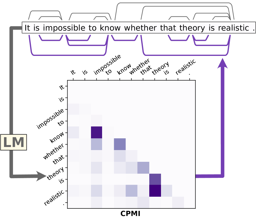
In this work, we dig further into the question of the correspondence between statistical and linguistic dependencies using modern pretrained language models (LMs) to compute estimates of conditional PMI between words given context, which we term contextualized pointwise mutual information (CPMI). For each sentence we extract a CPMI dependency tree, the spanning tree with maximum total CPMI, and compare these trees with gold standard linguistic dependency trees.111We release our code at https://github.com/mcqll/cpmi-dependencies.
We find that CPMI trees correspond better to gold standard trees than non context-dependent PMI trees. However our analysis shows that CPMI dependencies and linguistic dependencies correspond only roughly 50% of the time, even when we introduce a number of strong controls. Notably, we do not see better correspondence when we examine CPMI trees inferred by models that are explicitly trained to recover syntactic structure during training. Likewise, we see no increase in correspondence when we calculate CPMI over part-of-speech (POS) tags, a control designed to examine a less fine-grained statistical dependency than that between actual word forms. In fact, CPMI arcs broadly correspond to linguistic dependencies slightly less often than a simple baseline that just connects all and only adjacent words. We see similar overall unlabeled undirected attachment score (UUAS) when evaluated across a variety of pretrained models and different languages. However, a close analysis shows noteworthy differences between the different LMs, in particular revealing that BERT-based models are markedly more sensitive to adjacent words than XLNet. These differences yield insights about how different LM pretraining regimes result in differences in how the models allocate statistical dependencies between words in a sentence.
2 Background
Pointwise mutual information (PMI; Fano, 1961) is commonly used as a measure of the strength of statistical dependence between two words. Formally, PMI is a symmetric function of the probabilities of the outcomes of two random variables , which quantifies the amount of information about one outcome that is gained by learning the other:
In our case, the observations are two words in a sentence (drawn from discrete random variables indexed by position in the sentence, ranging over the vocabulary). PMI has been used in computational linguistic studies as a measure of how words inform each other’s probabilities since Church and Hanks (1989).222They used the term word association, which had a more subjective meaning in the psycholinguistic literature, to refer specifically to PMI.
Much earlier work on unsupervised dependency parsing (e.g., Van Der Mude and Walker, 1978; Magerman and Marcus, 1990; Carroll and Charniak, 1992; Yuret, 1998; Paskin, 2001) used techniques involving maximizing estimates of total pointwise mutual information between heads and dependents, or maximizing the conditional probability of dependents given heads (these two objectives can be shown to be equivalent under certain assumptions; see §C). While such PMI-induced dependencies proved useful for certain tasks (such as identifying the correct modifier for a word among a selection of possible choices; de Paiva Alves, 1996), purely PMI-based dependency parsers did not perform well at the general task of recovering linguistic structures overall (see discussion in Klein and Manning, 2004).
The recent advent of pretrained contextualized LMs (such as BERT, XLNet; Devlin et al., 2019; Yang et al., 2019) provides an opportunity to revisit the relationship between PMI-induced dependencies and linguistic dependencies. These networks are pretrained on very large amounts of natural language text using masked language modelling objectives to be accurate estimators of conditional probabilities of words given context, and thus are natural tools for investigating the statistical relationships between words.
3 Contextualized PMI dependencies
Linguistic dependencies are highly sensitive to context. For example, consider the following two sentences: I see that the crows retreated, and The mongoose pursued by crows retreated. In the first there is a dependency between retreated and crows, and in the second there is not. However, PMI between two words in a sentence is strictly independent of the other words in that sentence.
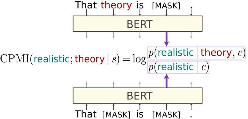
Here we define contextualized pointwise mutual information (CPMI) as the conditional PMI given context, which we estimate using pretrained contextualized LMs. A contextualized LM provides an estimate for the probability of words given context, which we use to define CPMIM between two words and in a sentence as
where the is the sentence with word masked, and is the sentence with words masked. To demonstrate the computation of this quantity, Figure 2 illustrates how BERT is used to obtain a CPMI score between the words theory and realistic in the sentence That theory is realistic.
3.1 Dependency tree induction
Given a sentence, we compute a matrix consisting of the CPMI between each pair of words. We then symmetrize this matrix by summing across the diagonal, so that we have a single score for each pair of words (omitting this step led to extremely similar results).333Note that while theoretically CPMI should be symmetric, nothing in the pretraining of the LMs we use enforces this identity (see §A.3.2 for details). We then extract tree structures which maximize total CPMI. Since natural language dependencies are overwhelmingly projective (see Kuhlmann, 2010) we extract maximum projective spanning trees using the dynamic programming algorithm from Eisner (1996, 1997).444Eisner’s algorithm recovers the optimal projective directed dependency structure from a weighted ordered graph, but with a symmetric weight matrix, the output dependency trees may be interpreted as undirected. Results for dependency trees alternatively extracted without the projectivity constraint, using Prim’s maximum spanning tree (MST) algorithm (Prim, 1957), are similar, and results using both algorithms are provided in §D for comparison. For further details on the extraction of CPMI dependencies, see §A.3.
Gold& was& nowhere& the& spectacular& performer& it& was& two& years& ago& on& Black& Monday& .
\depedge61nsubj
\depedge62cop
\depedge63advmod
\depedge64det
\depedge65amod
\depedge87nsubj
\depedge68rcmod
\depedge109num
\depedge1110npadvmod
\depedge811advmod
\depedge812prep
\depedge1413nn
\depedge1214pobj
\depedge[hide label, edge below, edge style=-, blue, opacity=0.5]1011
\depedge[hide label, edge below, edge style=-, blue, opacity=0.5]46
\depedge[hide label, edge below, edge style=-, blue, opacity=0.5]56
\depedge[hide label, edge below, edge style=-, blue, opacity=0.5]1314
\depedge[hide label, edge below, edge style=-, blue, opacity=0.5]910
\depedge[hide label, edge below, edge style=-, blue, opacity=0.5]78
\depedge[hide label, edge below, edge style=-, red, opacity=0.5]12
\depedge[hide label, edge below, edge style=-, red, opacity=0.5]67
\depedge[hide label, edge below, edge style=-, red, opacity=0.5]1213
\depedge[hide label, edge below, edge style=-, red, opacity=0.5]89
\depedge[hide label, edge below, edge style=-, red, opacity=0.5]23
\depedge[hide label, edge below, edge style=-, red, opacity=0.5]34
\depedge[hide label, edge below, edge style=-, red, opacity=0.5]1112
\node(R) at (\matrixref.east) ;
\node(R1) [right of = R] BERT-large;
\node(R4) at (R1.south) ;
{dependency}
{deptext}
Gold& was& nowhere& the& spectacular& performer& it& was& two& years& ago& on& Black& Monday& .
\depedge[hide label, edge below, edge style=-, blue, opacity=0.5]1011
\depedge[hide label, edge below, edge style=-, blue, opacity=0.5]1214
\depedge[hide label, edge below, edge style=-, blue, opacity=0.5]46
\depedge[hide label, edge below, edge style=-, blue, opacity=0.5]56
\depedge[hide label, edge below, edge style=-, blue, opacity=0.5]1314
\depedge[hide label, edge below, edge style=-, blue, opacity=0.5]910
\depedge[hide label, edge below, edge style=-, blue, opacity=0.5]78
\depedge[hide label, edge below, edge style=-, red, opacity=0.5]12
\depedge[hide label, edge below, edge style=-, red, opacity=0.5]67
\depedge[hide label, edge below, edge style=-, red, opacity=0.5]23
\depedge[hide label, edge below, edge style=-, red, opacity=0.5]1114
\depedge[edge unit distance=0.55ex,
hide label, edge below, edge style=-, red, opacity=0.5]711
\depedge[hide label, edge below, edge style=-, red, opacity=0.5]34
\node(R) at (\matrixref.east) ;
\node(R1) [right of = R] DistilBERT;
\node(R4) at (R1.south) ;
{dependency}
{deptext}
Gold& was& nowhere& the& spectacular& performer& it& was& two& years& ago& on& Black& Monday& .
\depedge[hide label, edge below, edge style=-, blue, opacity=0.5]1314
\depedge[hide label, edge below, edge style=-, blue, opacity=0.5]1214
\depedge[hide label, edge below, edge style=-, blue, opacity=0.5]46
\depedge[hide label, edge below, edge style=-, blue, opacity=0.5]910
\depedge[hide label, edge below, edge style=-, red, opacity=0.5]12
\depedge[hide label, edge below, edge style=-, red, opacity=0.5]67
\depedge[hide label, edge below, edge style=-, red, opacity=0.5]45
\depedge[edge unit distance=0.45ex,
hide label, edge below, edge style=-, red, opacity=0.5]38
\depedge[edge unit distance=0.55ex,
hide label, edge below, edge style=-, red, opacity=0.5]1014
\depedge[hide label, edge below, edge style=-, red, opacity=0.5]23
\depedge[hide label, edge below, edge style=-, red, opacity=0.5]34
\depedge[hide label, edge below, edge style=-, red, opacity=0.5]1112
\depedge[edge unit distance=0.35ex,
hide label, edge below, edge style=-, red, opacity=0.5]314
\node(R) at (\matrixref.east) ;
\node(R1) [right of = R] XLNet-base;
\node(R4) at (R1.south) ;
4 Evaluating CPMI dependencies
In this section, we analyze the degree to which CPMI-inferred dependencies from pretrained LMs resemble linguistic dependencies.
4.1 Method
We use gold dependencies for sentences from the Wall Street Journal (WSJ), from the Penn Treebank (PTB) corpus of English text hand-annotated for syntactic constituency parses (Marcus et al., 1994), converted into Stanford Dependencies (de Marneffe et al., 2006; de Marneffe and Manning, 2008b).555We use Stanford CoreNLP v3.9.2 to convert. We evaluate all extracted dependency trees on the full development split (WSJ section 22, consisting of 1700 sentences). For comparison with other work in unsupervised grammar induction, we also report results on the WSJ10 (all 389 sentences of length from section 23, the test split, as used in e.g. Yang et al. (2020)) in §D.1.
To compare results across languages we use the Parallel Universal Dependencies treebanks subset of Universal Dependencies (Nivre et al., 2020, v2.7). These consist of 1000 sentences translated into 20 languages.
Pretrained contextualized LMs
We compute CPMI scores using a number of transformer-based pretrained LMs for English (BERT, XLNet, XLM, BART, DistilBERT; Devlin et al., 2019; Yang et al., 2019; Conneau and Lample, 2019; Lewis et al., 2020; Sanh et al., 2019). For other languages (and English) we use pretrained multilingual BERT base; see D.2 for details. All pretrained contextualized LMs we use are provided by Hugging Face transformers (Wolf et al., 2020).
Syntactically aware models
We likewise compute CPMI estimates using models explicitly designed to have a linguistically-oriented inductive bias, by taking syntax into account in their training objectives and architecture. Following Du et al. (2020), we include two pretrained versions of an ordered-neuron LSTM (Shen et al., 2019)—a language model designed to have a hierarchical structural bias. The first (ONLSTM) is pretrained on raw text data, the second (ONLSTM-SYD) is pretrained on the same data but with an additional auxiliary objective to reconstruct PTB syntax trees. As a control, we also include a vanilla LSTM model. All three models are trained on the PTB training split. Example parses extracted from these models are given in the appendix (Figure 16). We extract CPMI estimates from these models similarly to the above, but we condition only on preceding material, since these LSTM-based models operate left-to-right. See §A.2 for details.666Note that results of the (ON)LSTM models are not directly comparable to the transformer-based models, as these models are trained on much less data.
Noncontextualized PMI control
We also compute a non-contextualized PMI estimate using a pretrained global word embedding model (Word2Vec; Mikolov et al., 2013), to capture word-to-word statistical relationships present in global distributional information, not sensitive to the context of particular sentences. This control is calculated as the inner product of Word2Vec’s target and context embeddings, , since its training objective is optimized when this quantity equals the PMI plus a global constant (as explained in Levy and Goldberg, 2014; Allen and Hospedales, 2019). Details are given in §A.1.
Baselines
A random baseline is obtained by extracting a parse for each sentence from a random matrix (so each pair of words is equally likely to be connected). We also include a ‘connect-adjacent’ baseline—degenerate trees formed by simply connecting the words in order—a simple, strong, and linguistically plausible baseline for English.
In addition to these baselines, we will compare unlabelled undirected accuracy score (UUAS) with that reported for the Dependency Model with Valence (DMV; Klein and Manning, 2004), a classic dependency parsing model. Note, importantly, the DMV is not fully unsupervised, as it relies on gold POS tags, but it is still a useful benchmark, with UUAS 54.4% on the entire WSJ corpus, and 63.7% on WSJ10 (as reported in Klein and Manning, 2004, Fig. 3).
4.2 Results
| all | len | len | |
|---|---|---|---|
| prec. rec. | prec. rec. | ||
| random | .22 | .49 .34 | .08 .10 |
| connect-adjacent | .49 | .49 1 | – 0 |
| Word2Vec | .39 | .61 .59 | .19 .19 |
| BERT base | .46 | .57 .72 | .27 .21 |
| BERT large | .47 | .55 .81 | .24 .13 |
| DistilBERT | .48 | .57 .72 | .32 .24 |
| Bart large | .38 | .52 .64 | .16 .13 |
| XLM | .42 | .60 .64 | .23 .22 |
| XLNet base | .45 | .59 .66 | .29 .25 |
| XLNet large | .41 | .59 .61 | .23 .22 |
| vanilla LSTM | .44 | .54 .70 | .26 .19 |
| ONLSTM | .44 | .55 .71 | .27 .19 |
| ONLSTM-SYD | .45 | .55 .71 | .27 .19 |
| language | rand. | connect-adj. | BERT base |
|---|---|---|---|
| Chinese | .23 | .45 | .40 |
| Czech | .25 | .48 | .48 |
| English | .22 | .42 | .43 |
| French | .23 | .45 | .47 |
| German | .22 | .42 | .46 |
| Korean | .28 | .58 | .49 |
| Polish | .27 | .54 | .52 |
| Russian | .26 | .51 | .51 |
| Spanish | .23 | .45 | .48 |
| Turkish | .27 | .55 | .48 |
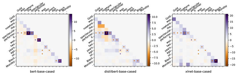
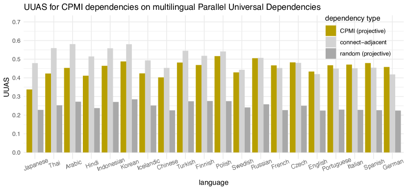
Example CPMI dependencies and extracted projective trees are given in Figure 3, with gold dependencies for comparison. Table 1 gives the UUAS results.777The overall UUAS constitutes both precision and recall, since the number of gold edges and CPMI edges are the same: for a sentence of length , the denominator is . Overall UUAS is given in the first column. The remaining columns give the UUAS for the subset of edges of length 1 and longer, in terms of precision and recall respectively.888For the connect-adjacent baseline, note: for length 1, the recall score is perfect, because all gold arcs of length 1 are predicted correctly by this trivial baseline; for the length subset, precision is undefined since there are no predicted edges of length , and recall is 0. Table 2 gives overall UUAS from multilingual BERT for a selection of languages from the PUD treebanks (for full results see Table 13, Figure 13).
The overall results show broadly that CPMI dependencies correspond to linguistic dependencies better than the noncontextual PMI-dependencies estimated from Word2Vec. However, across the models, and across languages, UUAS in general is in the range 40–50%. Degenerate trees formed by connecting words in linear order (the connect-adjacent baseline) achieve similar UUAS. Additionally, for the ONLSTM models, which have a hierarchical bias in their design, we see that accuracy of the CPMI-induced dependencies is the essentially the same with or without the auxiliary syntactic objective. Overall accuracy for both syntactically aware models is the same as for the vanilla LSTM. Further analysis of these results is in §6.
5 Delexicalized POS-CPMI dependencies
In this second experiment we estimate CPMI-dependencies over part-of-speech (POS) tags, rather than words. In the unsupervised dependency parsing literature there is an ample history of approaches making use of gold POS tags (see e.g., Bod, 2006; Cramer, 2007; Klein and Manning, 2004). Additionally, a traditional objection to the idea of deducing dependency structures directly from cooccurrence statistics, beyond data sparsity issues, is the possibility that “actual lexical items are too semantically charged to represent workable units of syntactic structure” (as phrased by Klein and Manning, 2004, p.3). That is, perhaps words’ patterns of co-occurrence contain simply too much information about factors irrelevant to dependency parsing, so as to drown out the information that would be useful for recovering dependency structure. According to this line of thinking, we might expect linguistic dependency structure to be better related to the statistical dependencies between the categories of words, rather than lexical items themselves. Thus a version of CPMI calculated over POS tags would be predicted to achieve higher accuracy than the CPMI calculated over lexical item probabilities above.
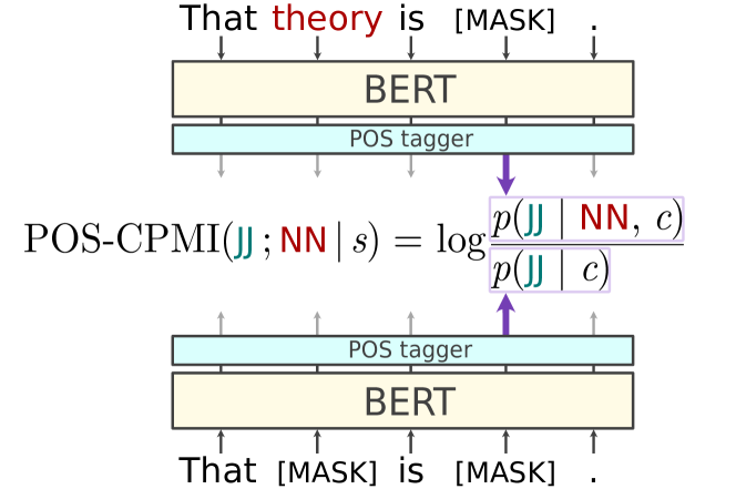
A straightforward but unfeasible way to investigate this idea would be to obtain contextualized POS-embeddings by re-training all the LMs from scratch on large delexicalized corpora only consisting of POS tags. Instead, for efficiency, follow LM probing literature (Hewitt and Manning, 2019) and train a small POS probe on top of a pretrained LM, which estimates the probability of the POS tag at a given position in a sentence. After training this probe, we can extract a POS-based CPMI score between words. We define this POS-CPMI analogously to CPMI, but using conditional probabilities of POS tags, rather than word tokens:
where are the gold POS tags of in sentence , and is the contextualized LM with a pretrained POS embedding network on top. This is illustrated in Figure 4. We then extract POS-CPMI dependencies to compare to gold dependencies.
5.1 Method
We implement a POS probe as a linear transformation on top of the final hidden layer of a fixed pretrained LM. We train two versions of this probe: one trained simply to minimize cross entropy loss (simple POS probe), the other trained using the information bottleneck technique (following Tishby et al., 2000; Li and Eisner, 2019), to maximize accuracy while minimizing extra information included in the representation (IB POS probe). Using LMs BERT and XLNet (both base and large, each), we train each type of probe, to recover PTB gold POS tags. All eight probes achieve between 92% and 98% training accuracy.
We extract parses from POS-CPMI matrices just for CPMI (described above in §4). Below, we refer to the estimates extracted using the simple POS probe as simple-POS-CPMI, and those extracted using the IB POS probe as IB-POS-CPMI.
5.2 Results
| all | len | len | ||
|---|---|---|---|---|
| prec. rec. | prec. rec. | |||
| BERT base | .48 | .56 .79 | .32 .19 | |
| BERT large | .45 | .53 .75 | .27 .16 | |
| XLNet base | .36 | .55 .56 | .17 .17 | |
| simple-POS | XLNet large | .32 | .56 .51 | .14 .15 |
| BERT base | .41 | .58 .65 | .20 .18 | |
| BERT large | .41 | .55 .69 | .18 .14 | |
| XLNet base | .40 | .55 .60 | .22 .20 | |
| IB-POS | XLNet large | .36 | .56 .56 | .16 .16 |
Using the POS-CPMI dependencies does not result in higher accuracy. This provides evidence that the correlation between linguistic dependencies and CPMI dependencies is not merely artificially low due to distracting lexical information.
Table 3 shows the UUAS of the simple-POS-CPMI and IB-POS-CPMI trees. Compared to the lexicalized CPMI trees discussed in the previous section, for BERT models, the simple-POS-CPMI dependencies have rather comparable overall UUAS, while for XLNet it is markedly lower. For both models, IB-POS-CPMI dependencies have lower UUAS. While these results are somewhat mixed, it is clear that, in our experimental setting, POS-CPMI dependencies correspond to gold dependencies no more than the CPMI dependencies do, performing at best roughly as well as the connect-adjacent baseline.
6 Analysis
In this section we outline main takeaways from a more detailed examination of the results from §§4–5, including additional analysis in §A.4.
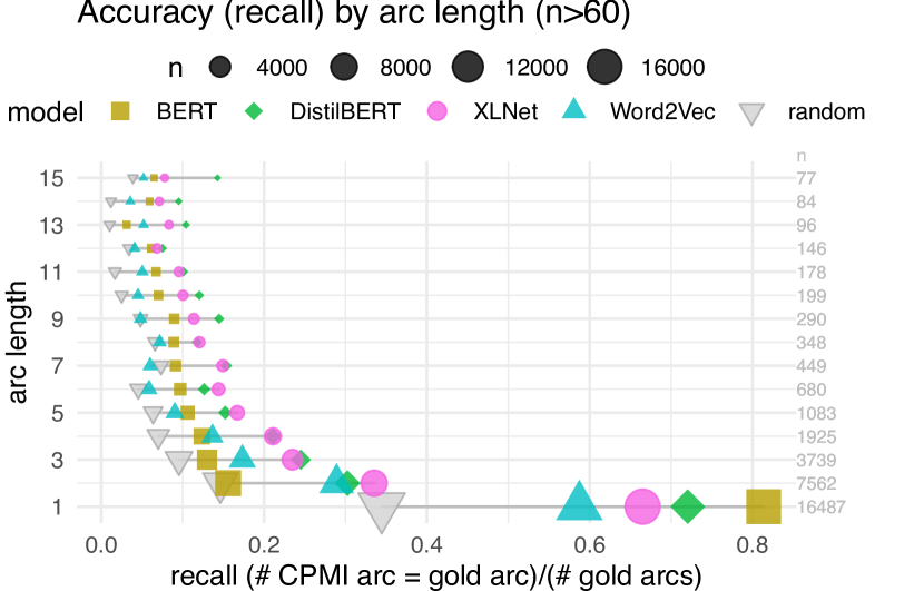
UUAS is higher for length 1 arcs
Breaking down the results by dependency length, Figure 8 (in appendix) shows the recall accuracy of CPMI dependencies, grouped by length of gold arc. Length 1 arcs have the highest accuracy, and longer dependencies have lower accuracy. This trend holds for CPMI from all LMs. For BERT large, in particular, arcs of length 1 have recall accuracy of 80%, while longer arcs are near random. For XLNet, this trend is less pronounced.
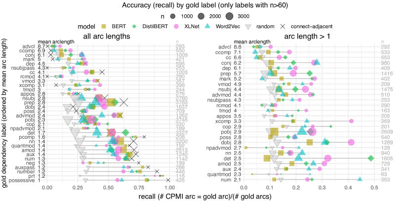
No relation label has high UUAS
In Figure 5, recall accuracy is plotted against gold dependency arc label.999For descriptions of labels see the Stanford Dependencies manual (de Marneffe and Manning, 2008a) When examining all lengths of dependency together (left) recall accuracy would seem to be correlated with mean arc length. But, filtering out all the gold arcs of length 1 (49% of arcs), we see that there is not a strong overall effect of arclength on mean accuracy for lengths > 1.
For most dependency labels, CPMI accuracy from each of the models is above the random baseline, but at or below to the connect-adjacent baseline. Exceptions to this trend include dependency labels dobj (direct object), xcomp (which connects a verb or adjective to the root of its clausal complement). For wordpairs in these relations, CPMI estimates (XLNet in particular) achieve higher accuracy than the baselines. However, even in these cases, CPMI dependencies do not perform at a level that could be considered successful for an unsupervised parser. This is contrary to what would be expected if CPMI-dependencies were in a strong correspondence with linguistic dependencies, even if this only held for certain types of linguistic dependency.
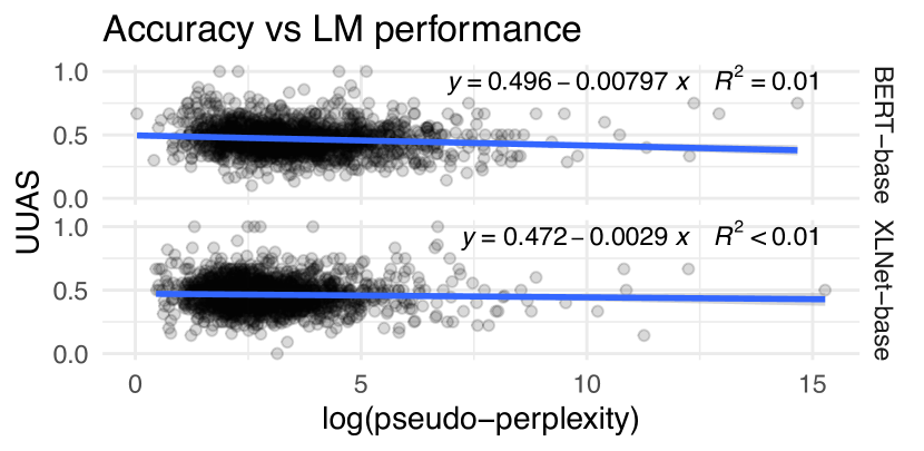
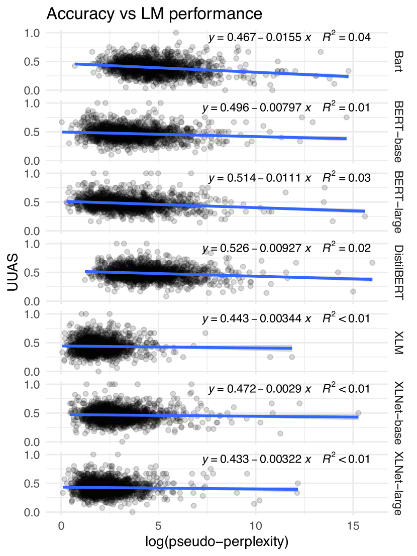
UUAS is not correlated with LM performance
Figure 6 shows per-sentence UUAS plotted against log pseudo-perplexity (PPL) for BERT and XLNet models (results are similar for other models; see §A.4.3, Figure 9). These results show that correspondence between CPMI-dependencies and linguistic dependencies isn’t higher on sentences on which the models are more confident.
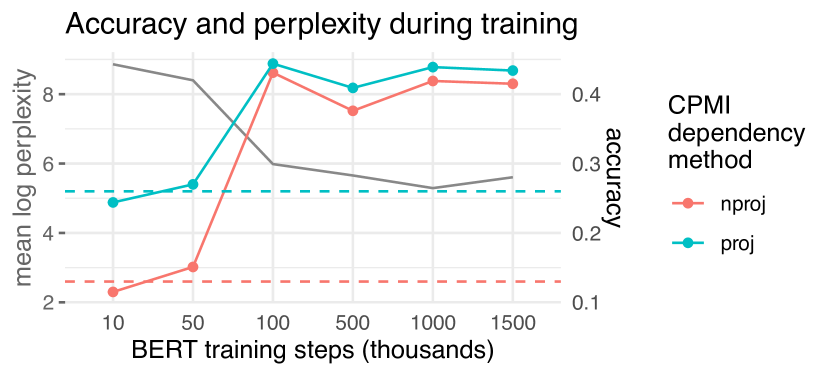
We also examined the accuracy of CPMI dependencies during training of BERT (base uncased) from scratch. Figure 11 (in appendix) shows the average perplexity of this model at checkpoints during training, along with average UUAS of induced CPMI structures. UUAS reaches its highest value before perplexity plateaus.
We should also stress that, throughout this paper, UUAS is not a measure of LM quality. Rather, it simply measures how well patterns of statistical dependence captured by the LM align with linguistic dependencies. Better alignment may not be related to better language modelling.
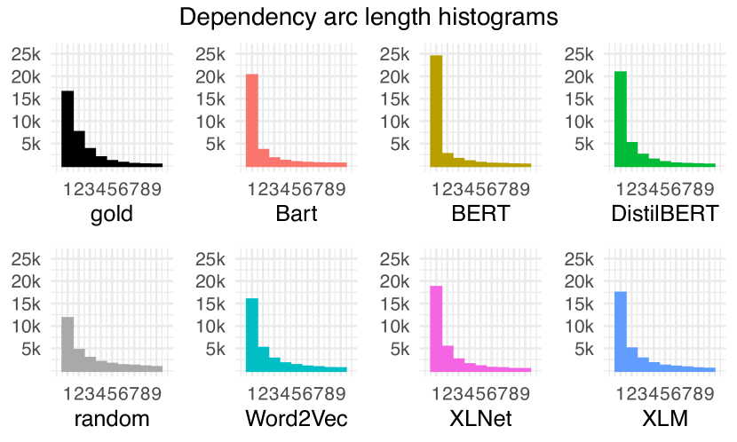
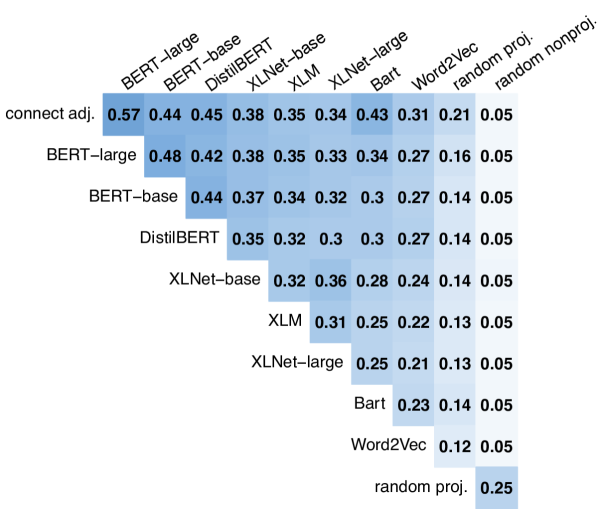
Dependencies differ between LMs
Dependency structures extracted from the different pretrained LMs show roughly similar overall UUAS, though the models agree with each other on only 25–48% of edges. They agree with the noncontextualized word embedding model Word2Vec at just slightly lower rates (21–27%), while agreeing with the linear baseline at higher rates (34–57%). See §A.4.1 and for these details.
In particular, CPMI dependencies from all the models connect adjacent words more often than the gold dependencies do, but this effect is much more pronounced for BERT models than for XLM, and XLNet models (Figure 7). A possible reason for this difference lies in the way these models are trained. XLNet is trained to predict words according to randomly sampled chain rule decompositions, enforcing a bias to be able to predict words in any order, including longer dependencies. XLNet’s probability estimates for words may therefore be sensitive to a larger set of words, rather than mostly the adjacent ones. Whereas BERT, trained with a less constrained masked LM objective, has probability estimates that are evidently more sensitive to adjacent words.
7 Related work
Probing pretrained embeddings
In the past few years, a substantial amount of literature has emerged on probing pretrained language models (in the sense of e.g. Conneau et al., 2018; Manning et al., 2020), wherein a presumably weak network (a probe) is trained to extract linguistic information (in particular, dependency information, in e.g. Hewitt and Manning, 2019; Clark et al., 2019) from pretrained embeddings. Extracting CPMI-dependencies differs from training a dependency probe in that it is entirely unsupervised, and is motivated by a specific hypothesis—about the relationship linguistic dependencies have with statistical dependence.
Nonparametric probing
A number of other recent works have taken an unsupervised approach to investigating syntactic structure encoded by pretrained LMs, largely focusing on self-attention weights (e.g. Mareček and Rosa, 2018, 2019; Kim et al., 2020a, b; Htut et al., 2019). Very recently, Zhang and Hashimoto (2021, concurrent with this paper) examined conditional dependencies implied by masked language modelling using a nonparametric method similar to our CPMI, using BERT to estimate Conditional PMI (and Conditional MI) between words. They extract maximum spanning trees, and report UUAS on WSJ dependency data. Their results are similar to those reported here: namely, scores are much higher than a chance baseline, but close to a connect-adjacent baseline. While their numerical results are similar, their interpretation differs somewhat. Given our analysis, we find less reason for optimism about the prospects of unsupervised dependency parsing directly from probability estimates by pretrained LMs.
Perturbation impact
The experiments in the current paper extracting CPMI can be seen as an application of the token perturbation approach of Wu et al. (2020). They describe general nonparametric method to examine the impact, , of a word on another word in the sentence, where is some difference function between the embedding of (masked in the input) with and without the word also being masked. In their experiments, they use two examples of impact-measuring functions (see Wu et al., 2020, §2.2). The first, the Dist metric, is simply Euclidean distance between embeddings. The second, the Prob metric, is defined as , using the masked LM’s probability estimates (notation as defined in §3). The latter impact metric is quite similar to CPMI, the difference being only that Prob impact is the difference in probabilities, while CPMI is the difference in log probabilities.
Table 4 compares the reported UUAS of maximum projective spanning trees from CPMI matrices, to those from Dist impact matrices on the English PUD data set. They do not report UUAS for the Prob metric or release code for it, but mention that it is significantly outperformed by the Dist method. Wu et al. (2020, p.1) note that their “best performing method does not go much beyond the strong right-chain baseline”. While it may be seen as an application of perturbed masking technique, CPMI is motivated as a method to test a specific hypothesis about the relationship between linguistic and statistical dependence. Extracting matrices using another impact metric (such as Euclidean distance between embeddings, Dist) may indeed achieve higher attachment scores, as Wu et al. (2020) demonstrate, but this does not bear on the hypothesis we focus on in this paper.
8 Discussion
In this paper we explored the connection between linguistic dependency and statistical dependence. We contribute a method to use modern pretrained language models to compute CPMI, a context-dependent estimate of PMI, and infer maximum CPMI dependency trees over sentences.
We find that these trees correlate with linguistic dependencies better than trees extracted from a noncontextual PMI estimate trained on similar data. However, we do not see evidence of a systematic correspondence between dependency arc label and the accuracy of CPMI arcs, nor do we see evidence that the correspondence increases when using models explicitly designed to encode linguistically-motivated inductive biases, nor when estimated between POS embeddings instead of word forms. Overall, CPMI-inferred dependencies correspond to gold dependencies no more than a simple baseline connecting adjacent words. This is our first main takeaway: statistical dependence (as modelled by these pretrained LMs) is not a good predictor of linguistic dependencies. Second, our analysis shows that CPMI trees extracted from different LMs differ to an extent that is perhaps surpising, given the similarity in spirit of their training regimes. The difference in accuracy when broken down with respect to linear distance between words offers information about the ways in which these models’ inductive and structural biases inform the way they perform the task of prediction. BERT aligns better overall, but this is driven by its being more like the linear baseline. For longer arcs, XLNet aligns a bit better with linguistic structure. Compared to BERT, XLNet can be seen as imposing a constraint on the language modelling objective by forcing the model to have accurate predictions under different permutation masks.
Generalizing this observation, we ask whether linguistic dependencies would correspond to the patterns of statistical dependence in a model trained with a language modelling loss while concurrently minimizing the amount of contextual information used to perform predictions. Finding ways of expressing such constraints on the amount of information used during prediction, and verifying the ways in which this can affect our results and LM pretraining in general constitutes material for future work.
| connect-adj. baseline | .42 |
| CPMI (proj.) BERT base multilingual cased | .43 |
| right-chain baseline | .40* |
| Dist impact (proj.) BERT base uncased | .52* |
| *As reported in Wu et al. (2020, Table 2) |
Acknowledgements
We thank anonymous reviewers, in particular the reviewer who alerted us to the work of Wu et al. (2020), and also Richard Futrell for helpful discussions and feedback. We also gratefully acknowledge support from the Centre for Research on Brain, Language & Music, the Natural Sciences and Engineering Research Council of Canada, the Fonds de Recherche du Québec, Nature et Technologies and Société et Culture, and the Canada CIFAR AI Chairs Program.
References
- Allen and Hospedales (2019) Carl Allen and Timothy M. Hospedales. 2019. Analogies explained: Towards understanding word embeddings. In Proceedings of the 36th International Conference on Machine Learning, ICML 2019, 9-15 June 2019, Long Beach, California, USA, volume 97 of Proceedings of Machine Learning Research, pages 223–231. PMLR.
- Bod (2006) Rens Bod. 2006. An all-subtrees approach to unsupervised parsing. In Proceedings of the 21st International Conference on Computational Linguistics and 44th Annual Meeting of the Association for Computational Linguistics, pages 865–872, Sydney, Australia. Association for Computational Linguistics.
- Carroll and Charniak (1992) Glenn Carroll and Eugene Charniak. 1992. Two experiments on learning probabilistic dependency grammars from corpora. AAAI Technical Report WS-92-01, AAAI.
- Church and Hanks (1989) Kenneth Ward Church and Patrick Hanks. 1989. Word association norms, mutual information, and lexicography. In 27th Annual Meeting of the Association for Computational Linguistics, pages 76–83, Vancouver, British Columbia, Canada. Association for Computational Linguistics.
- Clark et al. (2019) Kevin Clark, Urvashi Khandelwal, Omer Levy, and Christopher D. Manning. 2019. What does BERT look at? an analysis of BERT’s attention. In Proceedings of the 2019 ACL Workshop BlackboxNLP: Analyzing and Interpreting Neural Networks for NLP, pages 276–286, Florence, Italy. Association for Computational Linguistics.
- Conneau et al. (2018) Alexis Conneau, German Kruszewski, Guillaume Lample, Loïc Barrault, and Marco Baroni. 2018. What you can cram into a single $&!#* vector: Probing sentence embeddings for linguistic properties. In Proceedings of the 56th Annual Meeting of the Association for Computational Linguistics (Volume 1: Long Papers), pages 2126–2136, Melbourne, Australia. Association for Computational Linguistics.
- Conneau and Lample (2019) Alexis Conneau and Guillaume Lample. 2019. Cross-lingual language model pretraining. In Advances in Neural Information Processing Systems 32: Annual Conference on Neural Information Processing Systems 2019, NeurIPS 2019, December 8-14, 2019, Vancouver, BC, Canada, pages 7057–7067.
- Cramer (2007) Bart Cramer. 2007. Limitations of current grammar induction algorithms. In Proceedings of the ACL 2007 Student Research Workshop, pages 43–48, Prague, Czech Republic. Association for Computational Linguistics.
- de Marneffe et al. (2006) Marie-Catherine de Marneffe, Bill MacCartney, and Christopher D. Manning. 2006. Generating typed dependency parses from phrase structure parses. In Proceedings of the Fifth International Conference on Language Resources and Evaluation (LREC’06), Genoa, Italy. European Language Resources Association (ELRA).
- de Marneffe and Manning (2008a) Marie-Catherine de Marneffe and Christopher Manning. 2008a. Stanford typed dependencies manual. Stanford NLP.
- de Marneffe and Manning (2008b) Marie-Catherine de Marneffe and Christopher D. Manning. 2008b. The Stanford typed dependencies representation. In Coling 2008: Proceedings of the workshop on Cross-Framework and Cross-Domain Parser Evaluation, pages 1–8, Manchester, UK. Coling 2008 Organizing Committee.
- de Marneffe and Nivre (2019) Marie-Catherine de Marneffe and Joakim Nivre. 2019. Dependency grammar. Annual Review of Linguistics, 5(1):197–218.
- de Paiva Alves (1996) Eduardo de Paiva Alves. 1996. The selection of the most probable dependency structure in Japanese using mutual information. In 34th Annual Meeting of the Association for Computational Linguistics, pages 372–374, Santa Cruz, California, USA. Association for Computational Linguistics.
- Devlin et al. (2019) Jacob Devlin, Ming-Wei Chang, Kenton Lee, and Kristina Toutanova. 2019. BERT: Pre-training of deep bidirectional transformers for language understanding. In Proceedings of the 2019 Conference of the North American Chapter of the Association for Computational Linguistics: Human Language Technologies, Volume 1 (Long and Short Papers), pages 4171–4186, Minneapolis, Minnesota. Association for Computational Linguistics.
- Du et al. (2020) Wenyu Du, Zhouhan Lin, Yikang Shen, Timothy J. O’Donnell, Yoshua Bengio, and Yue Zhang. 2020. Exploiting syntactic structure for better language modeling: A syntactic distance approach. In Proceedings of the 58th Annual Meeting of the Association for Computational Linguistics, pages 6611–6628, Online. Association for Computational Linguistics.
- Eisner (1997) Jason Eisner. 1997. An empirical comparison of probability models for dependency grammar. Technical Report IRCS-96-11, Institute for Research in Cognitive Science, University of Pennsylvania.
- Eisner (1996) Jason M. Eisner. 1996. Three new probabilistic models for dependency parsing: An exploration. In COLING 1996 Volume 1: The 16th International Conference on Computational Linguistics.
- Fano (1961) Robert M Fano. 1961. Transmission of information: a statistical theory of communications. MIT Press.
- Futrell et al. (2019) Richard Futrell, Peng Qian, Edward Gibson, Evelina Fedorenko, and Idan Blank. 2019. Syntactic dependencies correspond to word pairs with high mutual information. In Proceedings of the Fifth International Conference on Dependency Linguistics (Depling, SyntaxFest 2019), pages 3–13, Paris, France. Association for Computational Linguistics.
- Hewitt and Liang (2019) John Hewitt and Percy Liang. 2019. Designing and interpreting probes with control tasks. In Proceedings of the 2019 Conference on Empirical Methods in Natural Language Processing and the 9th International Joint Conference on Natural Language Processing (EMNLP-IJCNLP), pages 2733–2743, Hong Kong, China. Association for Computational Linguistics.
- Hewitt and Manning (2019) John Hewitt and Christopher D. Manning. 2019. A structural probe for finding syntax in word representations. In Proceedings of the 2019 Conference of the North American Chapter of the Association for Computational Linguistics: Human Language Technologies, Volume 1 (Long and Short Papers), pages 4129–4138, Minneapolis, Minnesota. Association for Computational Linguistics.
- Htut et al. (2019) Phu Mon Htut, Jason Phang, Shikha Bordia, and Samuel R. Bowman. 2019. Do attention heads in BERT track syntactic dependencies?
- Kim et al. (2020a) Taeuk Kim, Jihun Choi, Daniel Edmiston, and Sang-goo Lee. 2020a. Are pre-trained language models aware of phrases? simple but strong baselines for grammar induction. In 8th International Conference on Learning Representations, ICLR 2020, Addis Ababa, Ethiopia, April 26-30, 2020. OpenReview.net.
- Kim et al. (2020b) Taeuk Kim, Bowen Li, and Sang goo Lee. 2020b. Chart-based zero-shot constituency parsing on multiple languages.
- Klein and Manning (2004) Dan Klein and Christopher Manning. 2004. Corpus-based induction of syntactic structure: Models of dependency and constituency. In Proceedings of the 42nd Annual Meeting of the Association for Computational Linguistics (ACL-04), pages 478–485, Barcelona, Spain.
- Kuhlmann (2010) Marco Kuhlmann. 2010. Dependency Structures and Lexicalized Grammars: An Algebraic Approach, volume 6270. Springer.
- Levy and Goldberg (2014) Omer Levy and Yoav Goldberg. 2014. Neural word embedding as implicit matrix factorization. In Advances in Neural Information Processing Systems 27: Annual Conference on Neural Information Processing Systems 2014, December 8-13 2014, Montreal, Quebec, Canada, pages 2177–2185.
- Lewis et al. (2020) Mike Lewis, Yinhan Liu, Naman Goyal, Marjan Ghazvininejad, Abdelrahman Mohamed, Omer Levy, Veselin Stoyanov, and Luke Zettlemoyer. 2020. BART: Denoising sequence-to-sequence pre-training for natural language generation, translation, and comprehension. In Proceedings of the 58th Annual Meeting of the Association for Computational Linguistics, pages 7871–7880, Online. Association for Computational Linguistics.
- Li and Eisner (2019) Xiang Lisa Li and Jason Eisner. 2019. Specializing word embeddings (for parsing) by information bottleneck. In Proceedings of the 2019 Conference on Empirical Methods in Natural Language Processing and the 9th International Joint Conference on Natural Language Processing (EMNLP-IJCNLP), pages 2744–2754, Hong Kong, China. Association for Computational Linguistics.
- Magerman and Marcus (1990) David M Magerman and Mitchell P Marcus. 1990. Parsing a natural language using mutual information statistics. In AAAI, volume 90, pages 984–989.
- Manning et al. (2020) Christopher D. Manning, Kevin Clark, John Hewitt, Urvashi Khandelwal, and Omer Levy. 2020. Emergent linguistic structure in artificial neural networks trained by self-supervision. Proceedings of the National Academy of Sciences, 117(48):30046–30054.
- Marcus et al. (1994) Mitchell Marcus, Grace Kim, Mary Ann Marcinkiewicz, Robert MacIntyre, Ann Bies, Mark Ferguson, Karen Katz, and Britta Schasberger. 1994. The Penn Treebank: Annotating predicate argument structure. In Human Language Technology: Proceedings of a Workshop held at Plainsboro, New Jersey, March 8-11, 1994.
- Mareček (2012) David Mareček. 2012. Unsupervised Dependency Parsing. MFF UK, Prague, Czech Republic. PhD Thesis.
- Mareček and Rosa (2018) David Mareček and Rudolf Rosa. 2018. Extracting syntactic trees from transformer encoder self-attentions. In Proceedings of the 2018 EMNLP Workshop BlackboxNLP: Analyzing and Interpreting Neural Networks for NLP, pages 347–349, Brussels, Belgium. Association for Computational Linguistics.
- Mareček and Rosa (2019) David Mareček and Rudolf Rosa. 2019. From balustrades to pierre vinken: Looking for syntax in transformer self-attentions. In Proceedings of the 2019 ACL Workshop BlackboxNLP: Analyzing and Interpreting Neural Networks for NLP, pages 263–275, Florence, Italy. Association for Computational Linguistics.
- Mikolov et al. (2013) Tomás Mikolov, Ilya Sutskever, Kai Chen, Gregory S. Corrado, and Jeffrey Dean. 2013. Distributed representations of words and phrases and their compositionality. In Advances in Neural Information Processing Systems 26: 27th Annual Conference on Neural Information Processing Systems 2013. Proceedings of a meeting held December 5-8, 2013, Lake Tahoe, Nevada, United States, pages 3111–3119.
- Nivre et al. (2020) Joakim Nivre, Marie-Catherine de Marneffe, Filip Ginter, Jan Hajič, Christopher D. Manning, Sampo Pyysalo, Sebastian Schuster, Francis Tyers, and Daniel Zeman. 2020. Universal Dependencies v2: An evergrowing multilingual treebank collection. In Proceedings of the 12th Language Resources and Evaluation Conference, pages 4034–4043, Marseille, France. European Language Resources Association.
- Paskin (2001) Mark A. Paskin. 2001. Grammatical bigrams. In Advances in Neural Information Processing Systems 14 [Neural Information Processing Systems: Natural and Synthetic, NIPS 2001, December 3-8, 2001, Vancouver, British Columbia, Canada], pages 91–97. MIT Press.
- Prim (1957) R. C. Prim. 1957. Shortest connection networks and some generalizations. The Bell System Technical Journal, 36(6):1389–1401.
- Řehůřek and Sojka (2010) Radim Řehůřek and Petr Sojka. 2010. Software Framework for Topic Modelling with Large Corpora. In Proceedings of the LREC 2010 Workshop on New Challenges for NLP Frameworks, pages 45–50, Valletta, Malta. ELRA.
- Salle and Villavicencio (2019) Alexandre Salle and Aline Villavicencio. 2019. Why so down? the role of negative (and positive) pointwise mutual information in distributional semantics.
- Sanh et al. (2019) Victor Sanh, Lysandre Debut, Julien Chaumond, and Thomas Wolf. 2019. DistilBERT, a distilled version of BERT: smaller, faster, cheaper and lighter.
- Shen et al. (2019) Yikang Shen, Shawn Tan, Alessandro Sordoni, and Aaron C. Courville. 2019. Ordered neurons: Integrating tree structures into recurrent neural networks. In 7th International Conference on Learning Representations, ICLR 2019, New Orleans, LA, USA, May 6-9, 2019. OpenReview.net.
- Tishby et al. (2000) Naftali Tishby, Fernando C. Pereira, and William Bialek. 2000. The information bottleneck method.
- Van Der Mude and Walker (1978) Antony Van Der Mude and Adrian Walker. 1978. On the inference of stochastic regular grammars. Information and Control, 38(3):310–329.
- Wolf et al. (2020) Thomas Wolf, Lysandre Debut, Victor Sanh, Julien Chaumond, Clement Delangue, Anthony Moi, Pierric Cistac, Tim Rault, Remi Louf, Morgan Funtowicz, Joe Davison, Sam Shleifer, Patrick von Platen, Clara Ma, Yacine Jernite, Julien Plu, Canwen Xu, Teven Le Scao, Sylvain Gugger, Mariama Drame, Quentin Lhoest, and Alexander Rush. 2020. Transformers: State-of-the-art natural language processing. In Proceedings of the 2020 Conference on Empirical Methods in Natural Language Processing: System Demonstrations, pages 38–45, Online. Association for Computational Linguistics.
- Wu et al. (2020) Zhiyong Wu, Yun Chen, Ben Kao, and Qun Liu. 2020. Perturbed masking: Parameter-free probing for analyzing and interpreting BERT. In Proceedings of the 58th Annual Meeting of the Association for Computational Linguistics, pages 4166–4176, Online. Association for Computational Linguistics.
- Yang et al. (2020) Songlin Yang, Yong Jiang, Wenjuan Han, and Kewei Tu. 2020. Second-order unsupervised neural dependency parsing. In Proceedings of the 28th International Conference on Computational Linguistics, pages 3911–3924, Barcelona, Spain (Online). International Committee on Computational Linguistics.
- Yang et al. (2019) Zhilin Yang, Zihang Dai, Yiming Yang, Jaime G. Carbonell, Ruslan Salakhutdinov, and Quoc V. Le. 2019. XLNet: Generalized autoregressive pretraining for language understanding. In Advances in Neural Information Processing Systems 32: Annual Conference on Neural Information Processing Systems 2019, NeurIPS 2019, December 8-14, 2019, Vancouver, BC, Canada, pages 5754–5764.
- Yuret (1998) Deniz Yuret. 1998. Discovery of Linguistic Relations Using Lexical Attraction. Ph.D. thesis, Massachusetts Institute of Technology, Dept. of Electrical Engineering and Computer Science.
- Zhang and Hashimoto (2021) Tianyi Zhang and Tatsunori Hashimoto. 2021. On the inductive bias of masked language modeling: From statistical to syntactic dependencies. Proceedings of the 2021 Conference of the North American Chapter of the Association for Computational Linguistics: Human Language Technologies.
Appendix A CPMI-dependency implementation details
A.1 Word2Vec as noncontextual PMI control
We use Word2Vec (Mikolov et al., 2013) to obtain a non-conditional PMI measure as a control/baseline. Additionally, in contrast with the CPMI values extracted from contextual language models, this estimate does not take into account the positions of the words in a particular sentence, but otherwise reflects global distributional information similarly to the contextualized models. Word2Vec should therefore function as a control with which to compare the PMI estimates derived from the contextualized models.
Word2Vec maps a given word in the vocabulary it to a ‘target’ embedding vector , as well as an ‘context’ embedding vector (used during training). As demonstrated by Levy and Goldberg (2014); Allen and Hospedales (2019), Word2Vec’s training objective is optimized when the inner product of the target and context embeddings equals the PMI, shifted by a global constant (determined by , the number of negative samples): This type of embedding model thus provides a non-contextual PMI estimator. A global shift will not change the resulting PMI-dependency trees, so we simply take , with embeddings calculated using a Word2Vec model trained on the same data as BERT.101010We use the implementation in Gensim (Řehůřek and Sojka, 2010), trained on BookCorpus and English Wikipedia, and use a global average vector for out-of-vocabulary words. Note: since we are ignoring the global shift of , an absolute valued version of PMI estimate will not be meaningful, and for this reason we only ever extract dependencies from the Word2Vec PMI estimate without taking the absolute value.
A.2 LtoR-CPMI for one-directional models
Our CPMI measure as defined above requires a bidirectional model (to calculate probabilities of words given their context, both preceding and following). The LSTM models we test in this study are left-to-right, so we define an slightly modified version of CPMI, to use with such unidirectional language models. That is, for a left to right model
where is the sentence up to before , and is the sentence up to before, with masked.
A.3 Calculating CPMI scores
A.3.1 Subtokenization
We must formulate the CPMI measure between sequences of subtokens, rather than tokens (words), because the large pretrained language models we use break down words into subtokens, for which gold dependencies and part of speech tags are not defined.
The calculation of CPMI between two lists of subtokens and in sentence is
where and are spans of (sub)token indices, is the set of subtokens with indices in (likewise for ), is the entire sentence without subtokens whose indices are in , and is the sentence without subtokens whose indices are in or .
Likewise, POS-CPMI is defined in terms of subtokens. Note that gold POS tags are defined for PTB word tokens, which may correspond to multiple subtokens. POS-CPMI is calculated as:
where is the contextual embedding model with a POS embedding network on top, and is the POS tag of (the set of subtokens with indices in , as in the definition of CPMI above).
To get the probability estimate for a multiple-subtoken word, we use a left-to-right chain rule decomposition. To get an estimate for a probability of a subtokenized word (that is, a joint probability, which we cannot get straight from a language model), we use a left-to-right chain rule decomposition of conditional probability estimates within the word:
This decomposition allows us to estimate conditional pointwise information between words made of multiple subtokens, at the expense of specifying a left-to-right order within those words.
A.3.2 Symmetrizing matrices
PMI is a symmetric function, but the estimated CPMI scores are not guaranteed to be symmetric, since nothing in the models’ training explicitly forces their conditionaly probability estimates of words given context to respect the identity . For this reason, we have a choice when assigning a score to a pair of words , whether we use the model’s estimate of , which compares the probability of with conditioner masked and unmasked, or of . In our implementation of CPMI we calculate scores in both directions, and use their sum (as mentioned in the main text §3.1), though experiments using one or the other (using just the upper or lower triangular of the matrix), or the max (equivalent to extracting a tree from the unsymmetrized matrix) led to very similar overall results. Likewise for the Word2Vec PMI estimate, and the POS-CPMI estimates.
A.3.3 Negative PMI values
PMI may be positive or negative. Results in the main text are all computed for CPMI dependencies extracted from signed matrices (so arcs with large negative CPMI will be rarely included). However, there is some discussion of interpreting the magnitude of PMI as indicating dependency, independent of sign (see Salle and Villavicencio, 2019). The choice to use an absolute-valued version of CPMI might be justified by arguing that words which influence each other’s distribution should be connected, whether this influence is positive or negative.
In §D.1 we include full results both with and without taking the absolute value of the CPMI matrices before extracting trees. The absolute-valued CPMI dependencies show a models increase in UUAS over the corresponding matrices without taking the absolute value in general. But, it is not clear whether the choice to use absolute-valued CPMI would be justified conceptually. Contrary to the conceptual motivation for CPMI dependencies, in which words which often occur together should be linked, an absolute-valued version links words which are highly informative of each others’ not being present. For this reason we do not choose to use an absolute-valued version of CPMI by default, but report those results for comparison, note that the UUAS is in fact higher with the absolute value, and refrain from further speculation.
A.4 Additional analysis of CPMI dependencies
A.4.1 Similarity between models
Figure 10 shows the similarity of the CPMI dependency structures extracted from the different contextual embedding models. We measure similarity of dependency structures with the Jaccard index for the sets of the predicted edges by two models. Jaccard index measures similarity of two sets and is defined as . The contextualized models agree with each other on around 30–50% of the edges, and agree with the the noncontextual baseline W2V slightly less. In general, they agree with the linear baseline at somewhat higher rates.
A.4.2 Accuracy versus arc length
Breaking down the results by dependency length, Figure 8 shows the recall accuracy of CPMI dependencies, grouped by length of gold arc. In general, length 1 arcs have the highest accuracy; longer dependencies have lower accuracy. CPMI dependencies from BERT (large) have 81% recall accuracy on length 1 arcs, with arcs longer than 1 having much lower recall (13% overall) near random (10%). In other models, XLNet in particular, this distinction is less of a binary distinction, but the trend is still for lower recall on longer arcs.
A.4.3 Accuracy versus perplexity
Here we investigate the correlation between language model performance and CPMI-dependency accuracy. If models’ confidence in predicting were tied to accuracy, it would be hard to argue that the relatively low accuracy score we see was due to the lack of connection between syntactic dependency and statistical dependency, rather than to the models’ struggling to recover such a structure. Here we measure model confidence by obtaining a perplexity score for each sentence, calculated as the negative mean of the pseudo log-likelihood, that is, for a sentence of length ,
Figure 9 shows that accuracy is not correlated with sentence-level perplexity for any of the models (fitting a linear regression, for each model). That is, the accuracy of CPMI-dependency structures is roughly the same on the sentences which the model predicts confidently (lower perplexity) as on the sentences which it predicts less confidently (higher perplexity).
A.4.4 UUAS during training
We examined the accuracy of CPMI dependencies during training of BERT (base uncased) from scratch. Figure 11 shows the average perplexity of this model, along with the sentence-wise average accuracy of CPMI structures at selected checkpoints during training. After about one million training steps the model has reached a plateau in terms of performance (perplexity stops decreasing), and we see that the peak UUAS has also plateaued at that point, but in fact reached its highest value after one hundred thousand training steps.
A.4.5 UUAS by dependency label
Table 5 gives per-dependency label recall accuracy of CPMI-dependencies extracted from the subset of dependency labels for which XLNet (base) achieves UUAS higher than both the linear and a random (projective) baselines.
| relation | meanlen | n | BERT | DistilBERT | Bart | XLNet | XLM | W2V | connect adj. | rand proj. |
|---|---|---|---|---|---|---|---|---|---|---|
| xcomp | 3.1 | 398 | 0.24 | 0.23 | 0.18 | 0.43 | 0.40 | 0.26 | 0.07 | 0.13 |
| mark | 5.0 | 421 | 0.18 | 0.29 | 0.11 | 0.30 | 0.20 | 0.09 | 0.05 | 0.10 |
| conj | 6.1 | 1009 | 0.12 | 0.19 | 0.21 | 0.28 | 0.26 | 0.29 | 0.03 | 0.10 |
| ccomp | 6.9 | 550 | 0.11 | 0.15 | 0.07 | 0.19 | 0.14 | 0.06 | 0.03 | 0.08 |
| dobj | 2.4 | 1637 | 0.37 | 0.38 | 0.33 | 0.47 | 0.42 | 0.35 | 0.21 | 0.16 |
| advcl | 8.7 | 293 | 0.05 | 0.04 | 0.05 | 0.11 | 0.07 | 0.06 | 0.00 | 0.06 |
| nsubjpass | 4.3 | 253 | 0.13 | 0.15 | 0.12 | 0.21 | 0.26 | 0.19 | 0.00 | 0.13 |
| rcmod | 4.1 | 290 | 0.11 | 0.07 | 0.12 | 0.12 | 0.14 | 0.11 | 0.00 | 0.08 |
| poss | 2.4 | 709 | 0.30 | 0.28 | 0.21 | 0.32 | 0.31 | 0.30 | 0.24 | 0.17 |
| pobj | 2.3 | 3745 | 0.33 | 0.39 | 0.28 | 0.36 | 0.32 | 0.30 | 0.30 | 0.17 |
| tmod | 3.0 | 244 | 0.31 | 0.35 | 0.30 | 0.39 | 0.40 | 0.18 | 0.33 | 0.18 |
| cop | 2.1 | 330 | 0.39 | 0.49 | 0.39 | 0.42 | 0.33 | 0.33 | 0.39 | 0.22 |
| det | 1.7 | 3327 | 0.52 | 0.64 | 0.24 | 0.53 | 0.43 | 0.41 | 0.52 | 0.23 |
Appendix B Information Bottleneck for POS probe
The simple POS probe is a -by--matrix, where the input dimension is the contextual embedding network’s hidden layer dimension, and the output dimension is the number of different POS tags in the tagset. Interpreting the output as an unnormalized probability distribution over POS tags, we train the layer to minimize the cross-entropy loss between the predicted and observed POS (using the labels from the Treebank). Training a simple linear probe is a rough way to get a compressed representations from contextual embeddings, but it has limitations (Hewitt and Liang, 2019).
A more correct way of extracting these representations is by a variational information bottleneck technique Tishby et al. (2000). We implement this technique (roughly following Li and Eisner, 2019), as follows. Optimization is to minimize , where is the input embedding, the latent representation and the true label. This technique trains two sets of parameters: the decoder, a linear model just as in the simple linear POS probe, and the encoder, another linear model, whose output in our case is interpreted as means and log-variances of a multivariate Gaussian (a simplifying assumption). Minimizing this loss maximizes information in the compressed representations about the output labels given a constraint on the amount of information that the compressed representations carry about the original embeddings.
Appendix C Equivalence of max pmi and max conditional probability objectives
Mareček (2012) describes the equivalence of optimizing for trees with maximum conditional probability of dependents given heads and optimizing for the maximum PMI between dependents and heads. This equivalence relies on an assumption that the marginal probability of words is independent of the parse tree.
For a corpus , a dependency structure can be described as a function which maps the index of a word to the index of its head. If net mutual information between dependents and heads according to dependency structure is , and the log conditional probability of dependents given heads is , the optimum is the same:
| (1) | ||||
| (2) | ||||
| (3) | ||||
| (4) |
The step taken in (3) follows only under the assumption that the marginal probability of dependent words is independent of the structure . That is, that “probabilities of the dependent words … are the same for all possible trees corresponding to a given sentence” (Mareček, 2012, §5.1.2). This must be stipulated as an assumption in a probabilistic model for the above derivation to hold.
Appendix D Augmented tables of results
We give results in further detail for the CPMI-dependencies on the English PTB Wall Street Journal (WSJ) and on the multilingual PUD treebanks. Tables described below follow this appendix.
D.1 Results on WSJ data
Results presented in this section repeat those given in the main text, with two independent additional parameters: projectivity and absolute value.
Projectivity
As described in §3.1, in the main text we report results for projective CPMI dependency trees extracted from CPMI matrices using Eisner’s algorithm Eisner (1996, 1997). These results are also repeated below, but we additionally present UUAS results for maximum spanning trees (MSTs) extracted from CPMI matrices using Prim’s algorithm (Prim, 1957), following Hewitt and Manning (2019).
Absolute value
In the main text we consider dependencies extracted from signed CPMI matrices. As described in §A.3.3, we also compute UUAS from absolute-valued matrices, and report them here.
In these tables, we also include the UUAS of randomized ‘lengthmatched’ control. For each sentence, this control consists of a randomized tree whose distribution of arc lengths is identical to the gold tree (obtained by rejection sampling).
D.1.1 WSJ10
Tables 9 and 9 give augmented UUAS results as in to Tables 7 and 7, resp., but for only the sentences of length from the test split (section 23) of the WSJ corpus (WSJ10). We include these results for comparison with much of the unsupervised dependency parsing literature following Klein and Manning (2004), which reports results on that subset. Note that the UUAS is naturally higher across the board on this corpus of shorter sentences.
| MSTs | Projective MSTs | |||||
| all | len | len | all | len | len | |
| prec. recall | prec. recall | prec. recall | prec. recall | |||
| random | .09 | .49 .10 | .05 .09 | .22 | .49 .34 | .08 .10 |
| connect-adjacent | .49 | .49 1 | – 0 | .49 | .49 1 | – 0 |
| lengthmatched | .37 | |||||
| Word2Vec | .27 | .67 .36 | .13 .19 | .39 | .61 .59 | .19 .19 |
| BERT base | .44 | .59 .68 | .26 .22 | .46 | .57 .72 | .27 .21 |
| BERT large | .46 | .56 .79 | .23 .14 | .47 | .55 .81 | .24 .13 |
| DistilBERT | .46 | .58 .68 | .30 .25 | .48 | .57 .72 | .32 .24 |
| Bart large | .36 | .53 .60 | .15 .14 | .38 | .52 .64 | .16 .13 |
| XLM | .38 | .64 .55 | .20 .22 | .42 | .60 .64 | .23 .22 |
| XLNet base | .42 | .61 .59 | .25 .26 | .45 | .59 .66 | .29 .25 |
| XLNet large | .36 | .63 .51 | .19 .22 | .41 | .59 .61 | .23 .22 |
| vanilla LSTM | .40 | .56 .60 | .23 .22 | .44 | .54 .70 | .26 .19 |
| ONLSTM | .41 | .57 .61 | .23 .22 | .44 | .55 .71 | .27 .19 |
| ONLSTM-SYD | .41 | .57 .61 | .23 .22 | .45 | .55 .71 | .27 .19 |
| MSTs | Projective MSTs | |||||
| all | len | len | all | len | len | |
| prec. recall | prec. recall | prec. recall | prec. recall | |||
| BERT base | .48 | .60 .75 | .29 .22 | .49 | .59 .78 | .31 .21 |
| BERT large | .48 | .56 .84 | .25 .13 | .48 | .56 .86 | .26 .13 |
| DistilBERT | .48 | .58 .73 | .32 .25 | .50 | .58 .77 | .35 .24 |
| Bart large | .38 | .55 .59 | .19 .17 | .40 | .54 .64 | .20 .16 |
| XLM | .41 | .65 .59 | .22 .24 | .44 | .63 .67 | .25 .23 |
| XLNet base | .44 | .61 .62 | .27 .26 | .47 | .60 .70 | .30 .25 |
| XLNet large | .37 | .63 .53 | .19 .23 | .42 | .61 .62 | .22 .22 |
| vanilla LSTM | .42 | .55 .63 | .25 .22 | .45 | .54 .73 | .28 .18 |
| ONLSTM | .42 | .56 .63 | .25 .22 | .45 | .54 .73 | .29 .19 |
| ONLSTM-SYD | .42 | .56 .64 | .25 .22 | .46 | .54 .74 | .29 .19 |
| MSTs | Projective MSTs | |||||
| all | len | len | all | len | len | |
| prec. recall | prec. recall | prec. recall | prec. recall | |||
| random | .29 | .56 .30 | .18 .28 | .34 | .54 .45 | .18 .21 |
| adjacent | .53 | .53 1 | – 0 | .53 | .53 1 | – 0 |
| lengthmatched | .51 | |||||
| Word2Vec | .42 | .61 .51 | .28 .32 | .46 | .60 .63 | .29 .27 |
| BERT base | .51 | .60 .69 | .36 .29 | .52 | .59 .72 | .38 .28 |
| BERT large | .52 | .59 .81 | .34 .20 | .53 | .59 .82 | .36 .20 |
| DistilBERT | .51 | .59 .71 | .38 .29 | .52 | .58 .75 | .40 .27 |
| Bart large | .44 | .54 .63 | .27 .21 | .45 | .54 .66 | .28 .21 |
| XLM | .48 | .61 .61 | .32 .32 | .49 | .60 .66 | .34 .31 |
| XLNet base | .51 | .61 .64 | .38 .35 | .53 | .60 .69 | .42 .35 |
| XLNet large | .46 | .61 .57 | .32 .34 | .48 | .59 .64 | .34 .31 |
| MSTs | Projective MSTs | |||||
| all | len | len | all | len | len | |
| prec. recall | prec. recall | prec. recall | prec. recall | |||
| BERT base | .53 | .60 .75 | .39 .28 | .54 | .60 .78 | .41 .27 |
| BERT large | .54 | .60 .85 | .37 .19 | .54 | .59 .86 | .38 .19 |
| DistilBERT | .54 | .60 .77 | .41 .28 | .55 | .60 .79 | .43 .27 |
| Bart large | .47 | .58 .63 | .31 .28 | .48 | .58 .67 | .33 .27 |
| XLM | .50 | .64 .65 | .33 .32 | .51 | .63 .69 | .35 .31 |
| XLNet base | .52 | .62 .68 | .39 .34 | .55 | .62 .73 | .42 .34 |
| XLNet large | .48 | .62 .61 | .33 .34 | .51 | .61 .66 | .37 .33 |
| MSTs | Projective MSTs | ||||||
| all | len | len | all | len | len | ||
| prec. recall | prec. recall | prec. recall | prec. recall | ||||
| BERT base | .47 | .57 .77 | .29 .20 | .48 | .56 .79 | .32 .19 | |
| BERT large | .44 | .54 .73 | .25 .17 | .45 | .53 .75 | .27 .16 | |
| XLNet base | .29 | .56 .41 | .14 .17 | .36 | .55 .56 | .17 .17 | |
| simple-POS | XLNet large | .26 | .59 .38 | .11 .15 | .32 | .56 .51 | .14 .15 |
| BERT base | .38 | .60 .58 | .18 .18 | .41 | .58 .65 | .20 .18 | |
| BERT large | .39 | .56 .64 | .17 .14 | .41 | .55 .69 | .18 .14 | |
| XLNet base | .36 | .57 .52 | .19 .20 | .40 | .55 .60 | .22 .20 | |
| IB-POS | XLNet large | .30 | .60 .44 | .13 .17 | .36 | .56 .56 | .16 .16 |
| MSTs | Projective MSTs | ||||||
| all | len | len | all | len | len | ||
| prec. recall | prec. recall | prec. recall | prec. recall | ||||
| BERT base | .49 | .57 .78 | .32 .21 | .50 | .57 .80 | .34 .21 | |
| BERT large | .47 | .56 .79 | .28 .17 | .48 | .55 .81 | .30 .16 | |
| XLNet base | .31 | .57 .44 | .15 .18 | .36 | .56 .56 | .17 .17 | |
| simple-POS | XLNet large | .27 | .59 .40 | .12 .15 | .31 | .57 .49 | .13 .14 |
| BERT base | .35 | .60 .52 | .16 .18 | .39 | .59 .61 | .19 .18 | |
| BERT large | .40 | .58 .67 | .17 .15 | .43 | .57 .72 | .19 .14 | |
| XLNet base | .38 | .58 .56 | .20 .21 | .42 | .57 .63 | .23 .21 | |
| IB-POS | XLNet large | .30 | .59 .44 | .13 .16 | .35 | .57 .55 | .16 .16 |
D.2 Results on multilingual PUD data
Table 13 gives results on the 20 languages of the Parallel Universal Dependencies (PUD) treebanks. These parallel treebanks were included in the CoNLL 2017 shared task on Multilingual Parsing from Raw Text to Universal Dependencies. The PUD treebank for each language consists of 1000 sentences annotated for Universal Dependencies. The sentences are translated into each of the languages, with the majority (750) being originally in English.
We compute CPMI for these sentences using the multilingual pretrained BERT-base model made available by Hugging Face Transformers (Wolf et al., 2020).111111https://huggingface.co/bert-base-multilingual-cased This model was trained using masked language modelling and next sentence prediction on the 104 languages with the largest Wikipedias, including all 20 in the PUD. UUAS for CPMI dependency trees for all languages is plotted in Figure 13.
| UUAS | ||||||||
|---|---|---|---|---|---|---|---|---|
| MSTs | Projective MSTs | |||||||
| language | mean sent. length | connect-adjacent | random | CPMI | CPMI (abs) | random | CPMI | CPMI (abs) |
| Arabic | 17.52 | .58 | .11 | .43 | .48 | .27 | .45 | .51 |
| Chinese | 17.51 | .45 | .11 | .38 | .39 | .23 | .40 | .42 |
| Czech | 14.99 | .48 | .12 | .47 | .48 | .25 | .48 | .50 |
| English | 17.73 | .42 | .10 | .41 | .43 | .22 | .43 | .45 |
| Finnish | 12.47 | .52 | .15 | .45 | .46 | .28 | .47 | .48 |
| French | 21.18 | .45 | .08 | .44 | .46 | .23 | .47 | .49 |
| German | 17.56 | .42 | .11 | .44 | .46 | .22 | .46 | .48 |
| Hindi | 20.53 | .51 | .09 | .38 | .39 | .24 | .41 | .42 |
| Icelandic | 15.88 | .49 | .12 | .40 | .41 | .25 | .42 | .44 |
| Indonesian | 16.06 | .56 | .12 | .44 | .46 | .27 | .46 | .49 |
| Italian | 20.43 | .45 | .09 | .45 | .46 | .23 | .47 | .48 |
| Japanese | 24.73 | .48 | .08 | .30 | .39 | .23 | .34 | .43 |
| Korean | 13.99 | .58 | .13 | .46 | .48 | .28 | .49 | .50 |
| Polish | 14.73 | .54 | .12 | .50 | .51 | .27 | .52 | .53 |
| Portuguese | 19.83 | .45 | .10 | .44 | .46 | .23 | .47 | .48 |
| Russian | 15.38 | .51 | .12 | .49 | .50 | .26 | .51 | .51 |
| Spanish | 20.00 | .45 | .09 | .46 | .47 | .23 | .48 | .50 |
| Swedish | 16.14 | .44 | .11 | .41 | .43 | .24 | .43 | .45 |
| Thai | 21.05 | .56 | .09 | .39 | .38 | .25 | .42 | .42 |
| Turkish | 13.73 | .55 | .14 | .46 | .48 | .27 | .48 | .50 |
It& is& impossible& to& know& whether& that& theory& is& realistic& .
\depedge31nsubj
\depedge32cop
\depedge54dep
\depedge35ccomp
\depedge106mark
\depedge87det
\depedge108nsubj
\depedge109cop
\depedge510ccomp
\depedge[hide label, edge below, edge style=-, blue, opacity=0.5]45
\depedge[hide label, edge below, edge style=-, blue, opacity=0.5]78
\depedge[hide label, edge below, edge style=-, blue, opacity=0.5]23
\depedge[hide label, edge below, edge style=-, blue, opacity=0.5]910
\depedge[hide label, edge below, edge style=-, red, opacity=0.5]12
\depedge[hide label, edge below, edge style=-, red, opacity=0.5]68
\depedge[hide label, edge below, edge style=-, red, opacity=0.5]56
\depedge[hide label, edge below, edge style=-, red, opacity=0.5]89
\depedge[hide label, edge below, edge style=-, red, opacity=0.5]34
\node(R) at (\matrixref.east) ;
\node(R1) [right of = R] Bart;
\node(R4) at (R1.south) ;
{dependency}
{deptext}
It& is& impossible& to& know& whether& that& theory& is& realistic& .
\depedge[hide label, edge below, edge style=-, blue, opacity=0.5]78
\depedge[hide label, edge below, edge style=-, blue, opacity=0.5]810
\depedge[hide label, edge below, edge style=-, blue, opacity=0.5]23
\depedge[hide label, edge below, edge style=-, red, opacity=0.5]68
\depedge[hide label, edge below, edge style=-, red, opacity=0.5]56
\depedge[hide label, edge below, edge style=-, red, opacity=0.5]89
\depedge[edge unit distance=0.5ex,
hide label, edge below, edge style=-, red, opacity=0.5]18
\depedge[hide label, edge below, edge style=-, red, opacity=0.5]36
\depedge[hide label, edge below, edge style=-, red, opacity=0.5]34
\node(R) at (\matrixref.east) ;
\node(R1) [right of = R] BERT-base;
\node(R4) at (R1.south) ;
{dependency}
{deptext}
It& is& impossible& to& know& whether& that& theory& is& realistic& .
\depedge[hide label, edge below, edge style=-, blue, opacity=0.5]45
\depedge[hide label, edge below, edge style=-, blue, opacity=0.5]610
\depedge[hide label, edge below, edge style=-, blue, opacity=0.5]23
\depedge[hide label, edge below, edge style=-, blue, opacity=0.5]910
\depedge[hide label, edge below, edge style=-, red, opacity=0.5]12
\depedge[hide label, edge below, edge style=-, red, opacity=0.5]67
\depedge[hide label, edge below, edge style=-, red, opacity=0.5]68
\depedge[hide label, edge below, edge style=-, red, opacity=0.5]56
\depedge[hide label, edge below, edge style=-, red, opacity=0.5]36
\node(R) at (\matrixref.east) ;
\node(R1) [right of = R] DistilBERT;
\node(R4) at (R1.south) ;
{dependency}
{deptext}
It& is& impossible& to& know& whether& that& theory& is& realistic& .
\depedge[hide label, edge below, edge style=-, blue, opacity=0.5]610
\depedge[hide label, edge below, edge style=-, blue, opacity=0.5]810
\depedge[hide label, edge below, edge style=-, blue, opacity=0.5]23
\depedge[hide label, edge below, edge style=-, blue, opacity=0.5]78
\depedge[hide label, edge below, edge style=-, blue, opacity=0.5]35
\depedge[hide label, edge below, edge style=-, red, opacity=0.5]56
\depedge[hide label, edge below, edge style=-, red, opacity=0.5]15
\depedge[hide label, edge below, edge style=-, red, opacity=0.5]34
\depedge[hide label, edge below, edge style=-, red, opacity=0.5]89
\node(R) at (\matrixref.east) ;
\node(R1) [right of = R] XLM;
\node(R4) at (R1.south) ;
{dependency}
{deptext}
It& is& impossible& to& know& whether& that& theory& is& realistic& .
\depedge[hide label, edge below, edge style=-, blue, opacity=0.5]45
\depedge[hide label, edge below, edge style=-, blue, opacity=0.5]610
\depedge[hide label, edge below, edge style=-, blue, opacity=0.5]810
\depedge[hide label, edge below, edge style=-, blue, opacity=0.5]910
\depedge[hide label, edge below, edge style=-, blue, opacity=0.5]23
\depedge[hide label, edge below, edge style=-, blue, opacity=0.5]78
\depedge[hide label, edge below, edge style=-, blue, opacity=0.5]35
\depedge[hide label, edge below, edge style=-, red, opacity=0.5]12
\depedge[hide label, edge below, edge style=-, red, opacity=0.5]56
\node(R) at (\matrixref.east) ;
\node(R1) [right of = R] XLNet-base;
\node(R4) at (R1.south) ;
{dependency}
{deptext}
It& is& impossible& to& know& whether& that& theory& is& realistic& .
\depedge[hide label, edge below, edge style=-, blue, opacity=0.5]910
\depedge[hide label, edge below, edge style=-, blue, opacity=0.5]78
\depedge[hide label, edge below, edge style=-, red, opacity=0.5]12
\depedge[hide label, edge below, edge style=-, red, opacity=0.5]69
\depedge[hide label, edge below, edge style=-, red, opacity=0.5]56
\depedge[hide label, edge below, edge style=-, red, opacity=0.5]89
\depedge[edge unit distance=0.45ex,
hide label, edge below, edge style=-, red, opacity=0.5]19
\depedge[hide label, edge below, edge style=-, red, opacity=0.5]36
\depedge[hide label, edge below, edge style=-, red, opacity=0.5]34
\node(R) at (\matrixref.east) ;
\node(R1) [right of = R] W2V-signed;
\node(R4) at (R1.south) ;
Gold& was& nowhere& the& spectacular& performer& it& was& two& years& ago& on& Black& Monday& .
\depedge61nsubj
\depedge62cop
\depedge63advmod
\depedge64det
\depedge65amod
\depedge87nsubj
\depedge68rcmod
\depedge109num
\depedge1110npadvmod
\depedge811advmod
\depedge812prep
\depedge1413nn
\depedge1214pobj
\depedge[hide label, edge below, edge style=-, blue, opacity=0.5]1011
\depedge[hide label, edge below, edge style=-, blue, opacity=0.5]46
\depedge[hide label, edge below, edge style=-, blue, opacity=0.5]56
\depedge[hide label, edge below, edge style=-, blue, opacity=0.5]1314
\depedge[hide label, edge below, edge style=-, blue, opacity=0.5]910
\depedge[hide label, edge below, edge style=-, blue, opacity=0.5]78
\depedge[hide label, edge below, edge style=-, red, opacity=0.5]12
\depedge[hide label, edge below, edge style=-, red, opacity=0.5]47
\depedge[edge unit distance=0.45ex,
hide label, edge below, edge style=-, red, opacity=0.5]313
\depedge[hide label, edge below, edge style=-, red, opacity=0.5]1213
\depedge[hide label, edge below, edge style=-, red, opacity=0.5]89
\depedge[hide label, edge below, edge style=-, red, opacity=0.5]23
\depedge[hide label, edge below, edge style=-, red, opacity=0.5]1112
\node(R) at (\matrixref.east) ;
\node(R1) [right of = R] Bart;
\node(R4) at (R1.south) ;
{dependency}
{deptext}
Gold& was& nowhere& the& spectacular& performer& it& was& two& years& ago& on& Black& Monday& .
\depedge[hide label, edge below, edge style=-, blue, opacity=0.5]1011
\depedge[hide label, edge below, edge style=-, blue, opacity=0.5]1214
\depedge[hide label, edge below, edge style=-, blue, opacity=0.5]46
\depedge[hide label, edge below, edge style=-, blue, opacity=0.5]56
\depedge[hide label, edge below, edge style=-, blue, opacity=0.5]1314
\depedge[hide label, edge below, edge style=-, blue, opacity=0.5]910
\depedge[hide label, edge below, edge style=-, blue, opacity=0.5]16
\depedge[hide label, edge below, edge style=-, blue, opacity=0.5]36
\depedge[hide label, edge below, edge style=-, blue, opacity=0.5]78
\depedge[hide label, edge below, edge style=-, red, opacity=0.5]611
\depedge[hide label, edge below, edge style=-, red, opacity=0.5]1112
\depedge[hide label, edge below, edge style=-, red, opacity=0.5]67
\depedge[hide label, edge below, edge style=-, red, opacity=0.5]23
\node(R) at (\matrixref.east) ;
\node(R1) [right of = R] BERT-base;
\node(R4) at (R1.south) ;
{dependency}
{deptext}
Gold& was& nowhere& the& spectacular& performer& it& was& two& years& ago& on& Black& Monday& .
\depedge[hide label, edge below, edge style=-, blue, opacity=0.5]1011
\depedge[hide label, edge below, edge style=-, blue, opacity=0.5]1214
\depedge[hide label, edge below, edge style=-, blue, opacity=0.5]46
\depedge[hide label, edge below, edge style=-, blue, opacity=0.5]56
\depedge[hide label, edge below, edge style=-, blue, opacity=0.5]1314
\depedge[hide label, edge below, edge style=-, blue, opacity=0.5]910
\depedge[hide label, edge below, edge style=-, blue, opacity=0.5]78
\depedge[hide label, edge below, edge style=-, red, opacity=0.5]12
\depedge[hide label, edge below, edge style=-, red, opacity=0.5]67
\depedge[hide label, edge below, edge style=-, red, opacity=0.5]23
\depedge[hide label, edge below, edge style=-, red, opacity=0.5]1114
\depedge[edge unit distance=0.55ex,
hide label, edge below, edge style=-, red, opacity=0.5]711
\depedge[hide label, edge below, edge style=-, red, opacity=0.5]34
\node(R) at (\matrixref.east) ;
\node(R1) [right of = R] DistilBERT;
\node(R4) at (R1.south) ;
{dependency}
{deptext}
Gold& was& nowhere& the& spectacular& performer& it& was& two& years& ago& on& Black& Monday& .
\depedge[hide label, edge below, edge style=-, blue, opacity=0.5]68
\depedge[hide label, edge below, edge style=-, blue, opacity=0.5]46
\depedge[hide label, edge below, edge style=-, blue, opacity=0.5]56
\depedge[hide label, edge below, edge style=-, blue, opacity=0.5]1314
\depedge[hide label, edge below, edge style=-, blue, opacity=0.5]16
\depedge[hide label, edge below, edge style=-, blue, opacity=0.5]36
\depedge[hide label, edge below, edge style=-, red, opacity=0.5]913
\depedge[hide label, edge below, edge style=-, red, opacity=0.5]67
\depedge[hide label, edge below, edge style=-, red, opacity=0.5]1213
\depedge[hide label, edge below, edge style=-, red, opacity=0.5]1013
\depedge[hide label, edge below, edge style=-, red, opacity=0.5]23
\depedge[hide label, edge below, edge style=-, red, opacity=0.5]1112
\depedge[hide label, edge below, edge style=-, red, opacity=0.5]614
\node(R) at (\matrixref.east) ;
\node(R1) [right of = R] XLM;
\node(R4) at (R1.south) ;
{dependency}
{deptext}
Gold& was& nowhere& the& spectacular& performer& it& was& two& years& ago& on& Black& Monday& .
\depedge[hide label, edge below, edge style=-, blue, opacity=0.5]1314
\depedge[hide label, edge below, edge style=-, blue, opacity=0.5]1214
\depedge[hide label, edge below, edge style=-, blue, opacity=0.5]46
\depedge[hide label, edge below, edge style=-, blue, opacity=0.5]910
\depedge[hide label, edge below, edge style=-, red, opacity=0.5]12
\depedge[hide label, edge below, edge style=-, red, opacity=0.5]67
\depedge[hide label, edge below, edge style=-, red, opacity=0.5]45
\depedge[edge unit distance=0.45ex,
hide label, edge below, edge style=-, red, opacity=0.5]38
\depedge[edge unit distance=0.55ex,
hide label, edge below, edge style=-, red, opacity=0.5]1014
\depedge[hide label, edge below, edge style=-, red, opacity=0.5]23
\depedge[hide label, edge below, edge style=-, red, opacity=0.5]34
\depedge[hide label, edge below, edge style=-, red, opacity=0.5]1112
\depedge[edge unit distance=0.35ex,
hide label, edge below, edge style=-, red, opacity=0.5]314
\node(R) at (\matrixref.east) ;
\node(R1) [right of = R] XLNet-base;
\node(R4) at (R1.south) ;
{dependency}
{deptext}
Gold& was& nowhere& the& spectacular& performer& it& was& two& years& ago& on& Black& Monday& .
\depedge[edge unit distance=0.55ex,
hide label, edge below, edge style=-, blue, opacity=0.5]26
\depedge[hide label, edge below, edge style=-, blue, opacity=0.5]1011
\depedge[hide label, edge below, edge style=-, blue, opacity=0.5]46
\depedge[hide label, edge below, edge style=-, blue, opacity=0.5]56
\depedge[hide label, edge below, edge style=-, blue, opacity=0.5]910
\depedge[hide label, edge below, edge style=-, blue, opacity=0.5]78
\depedge[edge unit distance=0.55ex,
hide label, edge below, edge style=-, red, opacity=0.5]27
\depedge[edge unit distance=0.35ex,
hide label, edge below, edge style=-, red, opacity=0.5]112
\depedge[edge unit distance=0.35ex,
hide label, edge below, edge style=-, red, opacity=0.5]113
\depedge[edge unit distance=0.35ex,
hide label, edge below, edge style=-, red, opacity=0.5]114
\depedge[edge unit distance=0.55ex,
hide label, edge below, edge style=-, red, opacity=0.5]810
\depedge[hide label, edge below, edge style=-, red, opacity=0.5]23
\depedge[edge unit distance=0.35ex,
hide label, edge below, edge style=-, red, opacity=0.5]212
\node(R) at (\matrixref.east) ;
\node(R1) [right of = R] W2V-signed;
\node(R4) at (R1.south) ;
“& We& have& sufficient& cash& flow& to& handle& that& ,& ”& he& said& .
\depedge32nsubj
\depedge[edge unit distance=0.45ex]133ccomp
\depedge64amod
\depedge65nn
\depedge36dobj
\depedge87aux
\depedge68vmod
\depedge89dobj
\depedge1312nsubj
\depedge[hide label, edge below, edge style=-, blue, opacity=0.5]56
\depedge[hide label, edge below, edge style=-, blue, opacity=0.5]78
\depedge[hide label, edge below, edge style=-, blue, opacity=0.5]1213
\depedge[hide label, edge below, edge style=-, blue, opacity=0.5]23
\depedge[hide label, edge below, edge style=-, red, opacity=0.5]913
\depedge[hide label, edge below, edge style=-, red, opacity=0.5]49
\depedge[hide label, edge below, edge style=-, red, opacity=0.5]67
\depedge[hide label, edge below, edge style=-, red, opacity=0.5]45
\depedge[hide label, edge below, edge style=-, red, opacity=0.5]34
\node(R) at (\matrixref.east) ;
\node(R1) [right of = R] Bart;
\node(R4) at (R1.south) ;
{dependency}
{deptext}
“& We& have& sufficient& cash& flow& to& handle& that& ,& ”& he& said& .
\depedge[hide label, edge below, edge style=-, blue, opacity=0.5]46
\depedge[hide label, edge below, edge style=-, blue, opacity=0.5]56
\depedge[hide label, edge below, edge style=-, blue, opacity=0.5]1213
\depedge[hide label, edge below, edge style=-, blue, opacity=0.5]23
\depedge[hide label, edge below, edge style=-, blue, opacity=0.5]78
\depedge[hide label, edge below, edge style=-, red, opacity=0.5]34
\depedge[hide label, edge below, edge style=-, red, opacity=0.5]67
\depedge[edge unit distance=0.45ex,
hide label, edge below, edge style=-, red, opacity=0.5]212
\depedge[edge unit distance=0.45ex,
hide label, edge below, edge style=-, red, opacity=0.5]29
\node(R) at (\matrixref.east) ;
\node(R1) [right of = R] BERT-base;
\node(R4) at (R1.south) ;
{dependency}
{deptext}
“& We& have& sufficient& cash& flow& to& handle& that& ,& ”& he& said& .
\depedge[hide label, edge below, edge style=-, blue, opacity=0.5]46
\depedge[hide label, edge below, edge style=-, blue, opacity=0.5]56
\depedge[hide label, edge below, edge style=-, blue, opacity=0.5]1213
\depedge[hide label, edge below, edge style=-, blue, opacity=0.5]89
\depedge[hide label, edge below, edge style=-, blue, opacity=0.5]23
\depedge[hide label, edge below, edge style=-, blue, opacity=0.5]78
\depedge[hide label, edge below, edge style=-, red, opacity=0.5]34
\depedge[hide label, edge below, edge style=-, red, opacity=0.5]47
\depedge[hide label, edge below, edge style=-, red, opacity=0.5]813
\node(R) at (\matrixref.east) ;
\node(R1) [right of = R] DistilBERT;
\node(R4) at (R1.south) ;
{dependency}
{deptext}
“& We& have& sufficient& cash& flow& to& handle& that& ,& ”& he& said& .
\depedge[hide label, edge below, edge style=-, blue, opacity=0.5]56
\depedge[hide label, edge below, edge style=-, blue, opacity=0.5]78
\depedge[hide label, edge below, edge style=-, blue, opacity=0.5]46
\depedge[hide label, edge below, edge style=-, blue, opacity=0.5]23
\depedge[edge unit distance=0.6ex,
hide label, edge below, edge style=-, red, opacity=0.5]48
\depedge[edge unit distance=0.45ex,
hide label, edge below, edge style=-, red, opacity=0.5]413
\depedge[edge unit distance=0.45ex,
hide label, edge below, edge style=-, red, opacity=0.5]412
\depedge[hide label, edge below, edge style=-, red, opacity=0.5]34
\depedge[edge unit distance=0.45ex,
hide label, edge below, edge style=-, red, opacity=0.5]912
\node(R) at (\matrixref.east) ;
\node(R1) [right of = R] XLM;
\node(R4) at (R1.south) ;
{dependency}
{deptext}
“& We& have& sufficient& cash& flow& to& handle& that& ,& ”& he& said& .
\depedge[hide label, edge below, edge style=-, blue, opacity=0.5]46
\depedge[hide label, edge below, edge style=-, blue, opacity=0.5]56
\depedge[hide label, edge below, edge style=-, blue, opacity=0.5]1213
\depedge[hide label, edge below, edge style=-, blue, opacity=0.5]23
\depedge[hide label, edge below, edge style=-, blue, opacity=0.5]78
\depedge[hide label, edge below, edge style=-, red, opacity=0.5]26
\depedge[hide label, edge below, edge style=-, red, opacity=0.5]67
\depedge[hide label, edge below, edge style=-, red, opacity=0.5]912
\depedge[hide label, edge below, edge style=-, red, opacity=0.5]79
\node(R) at (\matrixref.east) ;
\node(R1) [right of = R] XLNet-base;
\node(R4) at (R1.south) ;
{dependency}
{deptext}
“& We& have& sufficient& cash& flow& to& handle& that& ,& ”& he& said& .
\depedge[hide label, edge below, edge style=-, blue, opacity=0.5]46
\depedge[edge unit distance=0.4ex,
hide label, edge below, edge style=-, blue, opacity=0.5]313
\depedge[hide label, edge below, edge style=-, blue, opacity=0.5]56
\depedge[hide label, edge below, edge style=-, blue, opacity=0.5]1213
\depedge[hide label, edge below, edge style=-, blue, opacity=0.5]23
\depedge[edge unit distance=0.45ex,
hide label, edge below, edge style=-, red, opacity=0.5]913
\depedge[hide label, edge below, edge style=-, red, opacity=0.5]47
\depedge[hide label, edge below, edge style=-, red, opacity=0.5]34
\depedge[hide label, edge below, edge style=-, red, opacity=0.5]48
\node(R) at (\matrixref.east) ;
\node(R1) [right of = R] W2V-signed;
\node(R4) at (R1.south) ;
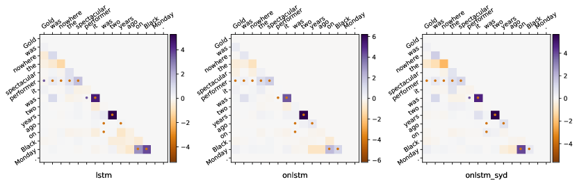
It& is& impossible& to& know& whether& that& theory& is& realistic& .
\depedge31nsubj
\depedge32cop
\depedge54dep
\depedge35ccomp
\depedge106mark
\depedge87det
\depedge108nsubj
\depedge109cop
\depedge510ccomp
\depedge[hide label, edge below, edge style=-, blue, opacity=0.5]13
\depedge[hide label, edge below, edge style=-, blue, opacity=0.5]610
\depedge[hide label, edge below, edge style=-, blue, opacity=0.5]910
\depedge[hide label, edge below, edge style=-, blue, opacity=0.5]78
\depedge[hide label, edge below, edge style=-, blue, opacity=0.5]35
\depedge[hide label, edge below, edge style=-, red, opacity=0.5]12
\depedge[hide label, edge below, edge style=-, red, opacity=0.5]89
\depedge[hide label, edge below, edge style=-, red, opacity=0.5]34
\depedge[hide label, edge below, edge style=-, red, opacity=0.5]56
\node(R) at (\matrixref.east) ;
\node(R1) [right of = R] LSTM;
\node(R4) at (R1.south) ;
{dependency}
{deptext}
It& is& impossible& to& know& whether& that& theory& is& realistic& .
\depedge[hide label, edge below, edge style=-, blue, opacity=0.5]910
\depedge[hide label, edge below, edge style=-, blue, opacity=0.5]13
\depedge[hide label, edge below, edge style=-, blue, opacity=0.5]35
\depedge[hide label, edge below, edge style=-, red, opacity=0.5]12
\depedge[hide label, edge below, edge style=-, red, opacity=0.5]67
\depedge[hide label, edge below, edge style=-, red, opacity=0.5]68
\depedge[hide label, edge below, edge style=-, red, opacity=0.5]56
\depedge[hide label, edge below, edge style=-, red, opacity=0.5]89
\depedge[hide label, edge below, edge style=-, red, opacity=0.5]34
\node(R) at (\matrixref.east) ;
\node(R1) [right of = R] ONLSTM;
\node(R4) at (R1.south) ;
{dependency}
{deptext}
It& is& impossible& to& know& whether& that& theory& is& realistic& .
\depedge[hide label, edge below, edge style=-, blue, opacity=0.5]910
\depedge[hide label, edge below, edge style=-, blue, opacity=0.5]13
\depedge[hide label, edge below, edge style=-, blue, opacity=0.5]78
\depedge[hide label, edge below, edge style=-, blue, opacity=0.5]35
\depedge[hide label, edge below, edge style=-, red, opacity=0.5]12
\depedge[hide label, edge below, edge style=-, red, opacity=0.5]69
\depedge[hide label, edge below, edge style=-, red, opacity=0.5]56
\depedge[hide label, edge below, edge style=-, red, opacity=0.5]89
\depedge[hide label, edge below, edge style=-, red, opacity=0.5]34
\node(R) at (\matrixref.east) ;
\node(R1) [right of = R] ONLSTM-SYD;
\node(R4) at (R1.south) ;
Gold& was& nowhere& the& spectacular& performer& it& was& two& years& ago& on& Black& Monday& .
\depedge61nsubj
\depedge62cop
\depedge63advmod
\depedge64det
\depedge65amod
\depedge87nsubj
\depedge68rcmod
\depedge109num
\depedge1110npadvmod
\depedge811advmod
\depedge812prep
\depedge1413nn
\depedge1214pobj
\depedge[hide label, edge below, edge style=-, blue, opacity=0.5]1214
\depedge[hide label, edge below, edge style=-, blue, opacity=0.5]46
\depedge[hide label, edge below, edge style=-, blue, opacity=0.5]56
\depedge[hide label, edge below, edge style=-, blue, opacity=0.5]1314
\depedge[hide label, edge below, edge style=-, blue, opacity=0.5]910
\depedge[hide label, edge below, edge style=-, blue, opacity=0.5]78
\depedge[hide label, edge below, edge style=-, red, opacity=0.5]12
\depedge[hide label, edge below, edge style=-, red, opacity=0.5]28
\depedge[hide label, edge below, edge style=-, red, opacity=0.5]810
\depedge[hide label, edge below, edge style=-, red, opacity=0.5]1012
\depedge[hide label, edge below, edge style=-, red, opacity=0.5]23
\depedge[hide label, edge below, edge style=-, red, opacity=0.5]34
\depedge[hide label, edge below, edge style=-, red, opacity=0.5]1112
\node(R) at (\matrixref.east) ;
\node(R1) [right of = R] LSTM;
\node(R4) at (R1.south) ;
{dependency}
{deptext}
Gold& was& nowhere& the& spectacular& performer& it& was& two& years& ago& on& Black& Monday& .
\depedge[hide label, edge below, edge style=-, blue, opacity=0.5]1214
\depedge[hide label, edge below, edge style=-, blue, opacity=0.5]46
\depedge[hide label, edge below, edge style=-, blue, opacity=0.5]56
\depedge[hide label, edge below, edge style=-, blue, opacity=0.5]1314
\depedge[hide label, edge below, edge style=-, blue, opacity=0.5]910
\depedge[hide label, edge below, edge style=-, blue, opacity=0.5]78
\depedge[hide label, edge below, edge style=-, red, opacity=0.5]12
\depedge[edge unit distance=0.45ex,
hide label, edge below, edge style=-, red, opacity=0.5]28
\depedge[edge unit distance=0.45ex,
hide label, edge below, edge style=-, red, opacity=0.5]114
\depedge[hide label, edge below, edge style=-, red, opacity=0.5]1014
\depedge[hide label, edge below, edge style=-, red, opacity=0.5]23
\depedge[hide label, edge below, edge style=-, red, opacity=0.5]1114
\depedge[hide label, edge below, edge style=-, red, opacity=0.5]34
\node(R) at (\matrixref.east) ;
\node(R1) [right of = R] ONLSTM;
\node(R4) at (R1.south) ;
{dependency}
{deptext}
Gold& was& nowhere& the& spectacular& performer& it& was& two& years& ago& on& Black& Monday& .
\depedge[hide label, edge below, edge style=-, blue, opacity=0.5]1011
\depedge[hide label, edge below, edge style=-, blue, opacity=0.5]1214
\depedge[hide label, edge below, edge style=-, blue, opacity=0.5]46
\depedge[hide label, edge below, edge style=-, blue, opacity=0.5]56
\depedge[hide label, edge below, edge style=-, blue, opacity=0.5]1314
\depedge[hide label, edge below, edge style=-, blue, opacity=0.5]910
\depedge[hide label, edge below, edge style=-, blue, opacity=0.5]78
\depedge[hide label, edge below, edge style=-, red, opacity=0.5]47
\depedge[hide label, edge below, edge style=-, red, opacity=0.5]14
\depedge[hide label, edge below, edge style=-, red, opacity=0.5]23
\depedge[hide label, edge below, edge style=-, red, opacity=0.5]710
\depedge[hide label, edge below, edge style=-, red, opacity=0.5]1114
\depedge[hide label, edge below, edge style=-, red, opacity=0.5]34
\node(R) at (\matrixref.east) ;
\node(R1) [right of = R] ONLSTM-SYD;
\node(R4) at (R1.south) ;
“& We& have& sufficient& cash& flow& to& handle& that& ,& ”& he& said& .
\depedge32nsubj
\depedge[edge unit distance=0.45ex]133ccomp
\depedge64amod
\depedge65nn
\depedge36dobj
\depedge87aux
\depedge68vmod
\depedge89dobj
\depedge1312nsubj
\depedge[hide label, edge below, edge style=-, blue, opacity=0.5]46
\depedge[hide label, edge below, edge style=-, blue, opacity=0.5]56
\depedge[hide label, edge below, edge style=-, blue, opacity=0.5]1213
\depedge[hide label, edge below, edge style=-, blue, opacity=0.5]23
\depedge[hide label, edge below, edge style=-, blue, opacity=0.5]78
\depedge[hide label, edge below, edge style=-, red, opacity=0.5]47
\depedge[edge unit distance=0.45ex,
hide label, edge below, edge style=-, red, opacity=0.5]212
\depedge[hide label, edge below, edge style=-, red, opacity=0.5]912
\depedge[hide label, edge below, edge style=-, red, opacity=0.5]24
\node(R) at (\matrixref.east) ;
\node(R1) [right of = R] LSTM;
\node(R4) at (R1.south) ;
{dependency}
{deptext}
“& We& have& sufficient& cash& flow& to& handle& that& ,& ”& he& said& .
\depedge[hide label, edge below, edge style=-, blue, opacity=0.5]56
\depedge[hide label, edge below, edge style=-, blue, opacity=0.5]23
\depedge[hide label, edge below, edge style=-, blue, opacity=0.5]78
\depedge[hide label, edge below, edge style=-, blue, opacity=0.5]1213
\depedge[hide label, edge below, edge style=-, red, opacity=0.5]67
\depedge[hide label, edge below, edge style=-, red, opacity=0.5]45
\depedge[edge unit distance=0.45ex,
hide label, edge below, edge style=-, red, opacity=0.5]212
\depedge[hide label, edge below, edge style=-, red, opacity=0.5]24
\depedge[edge unit distance=0.45ex,
hide label, edge below, edge style=-, red, opacity=0.5]912
\node(R) at (\matrixref.east) ;
\node(R1) [right of = R] ONLSTM;
\node(R4) at (R1.south) ;
{dependency}
{deptext}
“& We& have& sufficient& cash& flow& to& handle& that& ,& ”& he& said& .
\depedge[hide label, edge below, edge style=-, blue, opacity=0.5]56
\depedge[hide label, edge below, edge style=-, blue, opacity=0.5]23
\depedge[hide label, edge below, edge style=-, blue, opacity=0.5]78
\depedge[hide label, edge below, edge style=-, blue, opacity=0.5]1213
\depedge[hide label, edge below, edge style=-, red, opacity=0.5]67
\depedge[hide label, edge below, edge style=-, red, opacity=0.5]813
\depedge[hide label, edge below, edge style=-, red, opacity=0.5]45
\depedge[hide label, edge below, edge style=-, red, opacity=0.5]24
\depedge[hide label, edge below, edge style=-, red, opacity=0.5]912
\node(R) at (\matrixref.east) ;
\node(R1) [right of = R] ONLSTM-SYD;
\node(R4) at (R1.south) ;