Self-Supervised Pillar Motion Learning for Autonomous Driving
Abstract
Autonomous driving can benefit from motion behavior comprehension when interacting with diverse traffic participants in highly dynamic environments. Recently, there has been a growing interest in estimating class-agnostic motion directly from point clouds. Current motion estimation methods usually require vast amount of annotated training data from self-driving scenes. However, manually labeling point clouds is notoriously difficult, error-prone and time-consuming. In this paper, we seek to answer the research question of whether the abundant unlabeled data collections can be utilized for accurate and efficient motion learning. To this end, we propose a learning framework that leverages free supervisory signals from point clouds and paired camera images to estimate motion purely via self-supervision. Our model involves a point cloud based structural consistency augmented with probabilistic motion masking as well as a cross-sensor motion regularization to realize the desired self-supervision. Experiments reveal that our approach performs competitively to supervised methods, and achieves the state-of-the-art result when combining our self-supervised model with supervised fine-tuning.
1 Introduction
Understanding††This work was done while C. Luo was interning at QCraft. the motion of various traffic agents is crucial for self-driving vehicles to be able to safely operate in dynamic environments. Motion provides pivotal information to facilitate a variety of onboard modules ranging from detection, tracking, prediction to planning. A self-driving vehicle is typically equipped with multiple sensors, and the most commonly used one is LiDAR. How to represent and extract temporal motion from point clouds is therefore one of the fundamental research problems in autonomous driving [9, 20, 39]. This is however challenging in the sense that (1) there exist numerous agent categories and each category exhibits specific motion behavior; (2) point cloud is sparse and lacks of exact correspondence between sweeps; and (3) estimating process is required to meet tight runtime constraint and limited onboard computation.
A traditional autonomy stack usually performs motion estimation by first recognizing other traffic participants in the scene and then predicting how the scene might progress given their current states [9, 18]. However, most recognition models are only trained to classify and localize objects from a handful of known categories. This closed-set scenario is apparently insufficient for a practical autonomy system to perceive motion of a large diversity of instances that are not seen during training. As the lower-level information compared to object semantics, motion should be ideally estimated in an open-set setting irrespective of whether objects belong to a known or unknown category. One appealing way to predict class-agnostic motion is to estimate scene flow from point clouds by estimating the 3D velocity of each point [20, 24]. Unfortunately, this dense motion filed prediction is currently computationally prohibitive to process one complete LiDAR sweep, ruling out the practical use for self-driving vehicles that require real-time and large-scale point cloud processing.
Another possibility to represent and estimate motion is based on bird’s eye view (BEV). In this way, a point cloud is discretized into grid cells, and motion information is described by encoding each cell with a 2D displacement vector indicating the position into the future of the cell on the ground plane [8, 17, 39]. This compact representation successfully simplifies scene motion as the motion taking place on the ground plane is the primary concern for autonomous driving, while the motion in the vertical direction is not as much important or useful. Additionally, point clouds represented in this form are efficient since all key operations can be conducted via 2D convolutions that are extremely fast to compute on GPUs. Recent works also show that this representation can be readily generalized to class-agnostic motion estimation [8, 17]. However, they have to rely on large amounts of annotated point cloud data with object detection and tracking as proxy motion supervision, which is expensive and difficult to obtain in practice.
Statistics finds that a self-driving vehicle generates over 1 terabyte of data per day but only less than 5% of the data is used [1]. Thus, learning without requiring manual labeling is of critical importance in order to fully harness the abundant data. While the recent years have seen growing interests in self-supervised learning for language [5, 15] and vision [14, 34], self-supervision for point clouds still falls behind, yet has great potential to open up the possibility to utilize practically infinite training data that is continuously collected by the world-wide self-driving fleets.
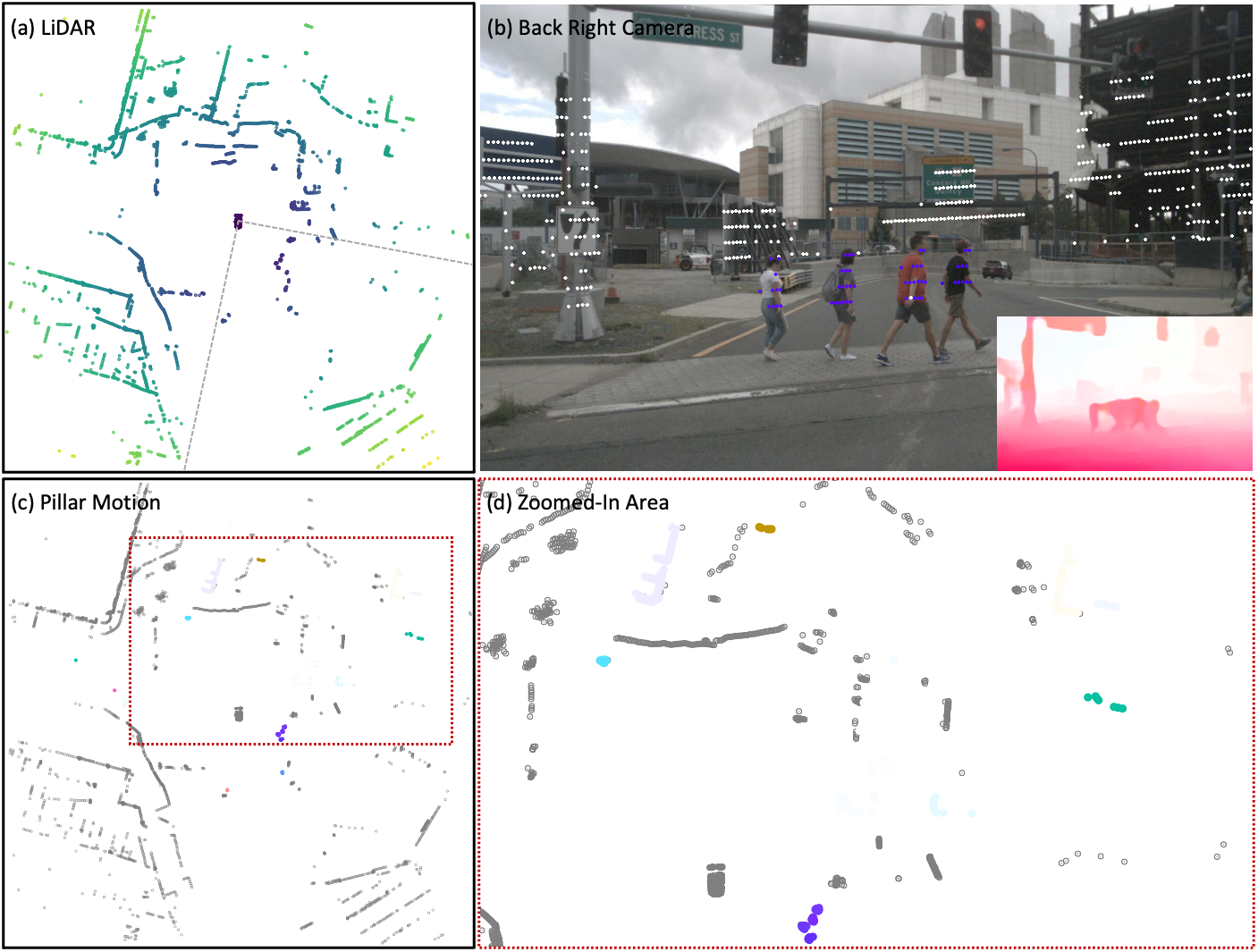
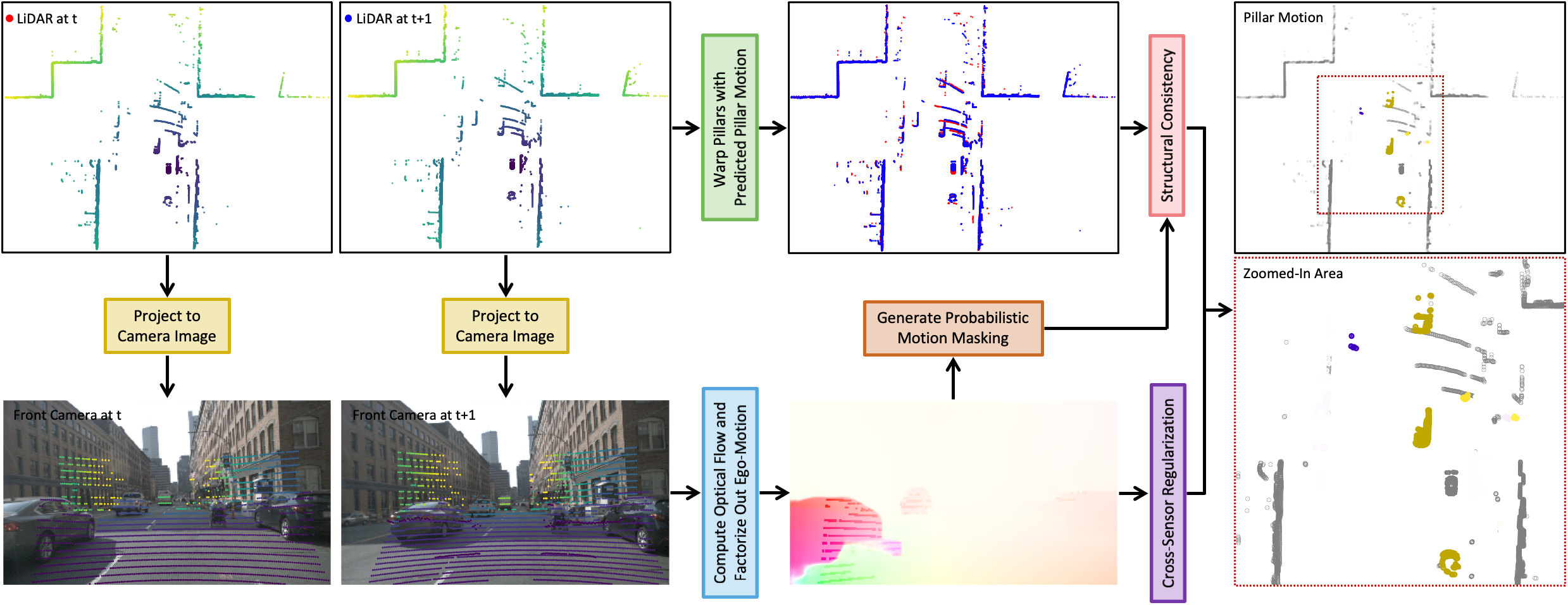
In light of the above observations, we propose a self-supervised learning framework that exploits free supervisory signals from multiple sensors for open-set motion estimation, as shown in Figure 1. To take advantage of the merits of motion representation in BEV, we organize a point cloud into pillars (i.e., vertical columns) [16], and refer to the velocity associated with each pillar as pillar motion. We introduce a point cloud based self-supervision by assuming pillar or object structure constancy between two consecutive sweeps. However, this does not hold in most cases due to the lack of exact point correspondence caused by the sparse scans of LiDAR. Our solution towards mitigating this difficulty is to make use of optical flow extracted from camera images to provide self-supervised and cross-sensory regularization. As illustrated in Figure 2, this design leads to a unified learning framework that subsumes the interactions between LiDAR and the paired cameras: (1) point clouds facilitate factorizing ego-motion out from optical flow; (2) image motion provides auxiliary regularization for learning pillar motion in point clouds; (3) probabilistic motion masking formed by back-projected optical flow promotes structural consistency in point clouds. Note that the camera-related components are only used in training and discarded for inference, thus no additional computations are introduced for the camera modality at runtime.
To our knowledge, this work provides the first learning paradigm that is able to perform pillar motion prediction in a fully self-supervised framework. We propose novel self-supervisory and cross-sensory signals by tightly integrating point clouds and paired camera images to achieve the desired self-supervision. Experiments show that our approach compares favorably to the existing supervised methods. Our code and model will be made available at https://github.com/qcraftai/pillar-motion.
2 Related Work
Motion Estimation. This task aims to estimate motion dynamics and predict future locations of various agents via past observations. Traditional approaches typically formulate this task as a trajectory forecasting problem that hinges on perception outputs from 3D object detection and tracking [9, 18]. As a result of the dependence on the related modules, such a paradigm is prone to detection and tracking errors [17] and lacks the ability to tackle unknown object classes [38]. Another active research line is to estimate scene flow from point clouds to understand the dense 3D motion field [11, 20]. However, current methods often take hundreds of milliseconds to process a partial point cloud, which is even though significantly subsampled. Moreover, the dense supervision of ground truth scene flow is hard to acquire in real data [24, 40]. Thus, these methods operate on either synthetic data (FlyingThings3D [23]) or densely processed data (KITTI Scene Flow [10]), where dense point correspondences are mostly available. However, for the raw point clouds scanned by LiDAR, such correspondences usually do not exist, making it more difficult to directly estimate scene flow from LiDAR.
Several recent methods are proposed to explore estimating motion in BEV to simplify the understanding of scene motion. MotionNet is proposed in [39] to perform joint perception and motion prediction based on a spatio-temporal pyramid network with three correlated heads. A differentiable ego-motion compensation layer [8] is introduced to augment a recurrent convolutional network [42] for temporal context aggregation. In [17] an optical flow network adapted from [32] is used to learn correspondence matching between two consecutive point clouds. Compared to these works that rely on large labeled training data with 3D detection and tracking to approximate motion supervision, we aim to learn pillar motion from unlabeled data collections in a fully self-supervised manner.
Self-Supervised Learning. To take advantage of the vast amount of unlabeled images and videos, numerous methods have been developed for different tasks using various self-supervised losses. For the feature representation learning, geometric or color transformation [14, 34], contrastive learning [44], frame interpolation [26], and sequence ordering [7] have been widely explored. As for optical flow estimation [37], photometric constancy over time and spatial smoothness of flow fields are also well studied. In [45] the differentiable rendering and autoencoding reconstruction are applied to discover object attributes, such as 3D shape, landmarks, part segmentation, and camera viewpoint.
All these studies are conducted in the context of images and videos, while self-supervision in point clouds has been less explored. PointContrast [41] presents a unified triplet of architecture and contrastive loss for pre-training, and transfers the learned 3D feature representations to point cloud segmentation and detection tasks. Mittal et al. [24] present a method to train scene flow by combining two self-supervised losses based on nearest neighbors and temporal consistency. It is proposed in [40] to further incorporate smoothness constraints and Laplacian coordinates to preserve local structure for scene flow training. Different from the previous works, we focus on pillar motion learning and leveraging complementary self-supervision from point clouds and associated camera images.
LiDAR and Camera Fusion. A large family of the multi-sensor fusion research is about 3D object detection. For object-centric methods [4], fusion is conducted at the object proposal level by roi-pooling features from separate backbone networks of camera and LiDAR. In [19] continuous feature fusion is developed to allow feature sharing across all levels of the backbones of two modalities with a sophisticated mapping between point clouds and images. A detection seeding scheme is employed in [28] to extract image semantics from detection or segmentation to seed detection in point clouds. PointPainting [35] presents a simple and sequential fusion method that projects points onto the output of an image based semantic segmentation network and appends the class scores to each point.
Some recent works employ very sparse (hundreds to thousands) LiDAR measurements to enhance image based dense scene flow estimation. Sparse LiDAR is integrated with stereo images in [2] to resolve the lack of information in challenging image regions caused by shadows, poor illumination, and textureless objects. Rishav et al. [29] further extend this method to a monocular camera setup through a late feature fusion at multiple scales and demonstrate superior performance over image-only methods. In contrast, we propose a cross-sensor based self-supervision to regularize motion learning in point clouds by alleviating the lack of exact correspondences between sweeps.
3 Method
As illustrated in Figure 2, the proposed motion learning approach tightly couples the self-supervised structural consistency from point clouds and the cross-sensor motion regularization. Our regularization involves factorizing out ego-motion from optical flow and enforcing motion agreement across sensors. We also introduce a probabilistic motion masking based on the back-projected optical flow to enhance structural similarity matching in point clouds.
3.1 Problem Formulation
Given a temporal sequence of self-driving keyframes, we denote the point cloud and the paired camera images captured at time as and , where indicates a point and is the number of received points, denotes an image and is the number of cameras in the sensor suite mounted on a self-driving vehicle. In the following we omit the camera index and use to indicate any camera image for brevity. is discretized into non-overlapping pillars , where denotes a pillar index and is the number of pillars. We define the pillar motion field as the movement of each pillar to its corresponding position at next timestamp: , . is defined such that and represent the same part of a scene moving in time. is a locally rigid and non-deforming motion field, which assumes that all dynamics are on ground plane and the motion is consistent for every point inside a pillar.
3.2 LiDAR based Structural Consistency
According to the above definition of pillar motion , we assign the motion vector of each pillar to all the points within the pillar to obtain the per point motion, and simply set the motion along the vertical direction to be zero. After having the per point motion, we can transform the original point cloud to the next timestamp and get . Since there is no ground truth motion available, we instead to seek to use the structural consistency between the transformed point cloud and the real point cloud as free supervision to guide the pillar motion learning.
We take inspiration from the chamfer matching for image registration [12] and measure the structural similarity between two point clouds and as:
| (1) |
Here we leave out the time index for brevity. Conceptually, this self-supervised structural consistency loss makes use of the nearest neighbor distances between transformed points and real points of the two point clouds and to approximate the pillar motion filed.
Apparently this structural consistency relies on the existence of corresponding points between two consecutive point clouds and . However, for the raw scans of LiDAR, this assumption does not usually hold for a number of cases. For example, the corresponding points cannot be exactly re-scanned at the next timestamp, and they can be occluded or fall out of the sensor range. These scenarios become even worse for the objects at distance, where the points are extremely sparse. As can be seen from the projected points on the two camera images in Figure 2, the scanned points on the back of the distant bus over the two sweeps do not correspond exactly. And the nearest neighbor matching can be ambiguous within cluster of points. Therefore, we argue that directly forcing the model to conduct the nearest neighbor based structural matching between two point clouds would inevitably introduce noise.
3.3 Cross-Sensor Motion Regularization
As aforementioned, the nearest neighbor based structural consistency can cause ambiguity when point clouds are sufficiently sparse, as is common for the widely used sparse LiDAR. On the other hand, cameras in a sensor suite provide complementary appearance cues and more dense information. Thus, it would be helpful to incorporate image information along with LiDAR. One solution is to estimate scene flow from images also in an self-supervised manner. However, estimating scene flow directly from camera images is still hard and inaccurate, while optical flow estimation is relatively more precise and mature. So we instead relax the regularization by projecting predicted pillar motion onto image planes and utilize optical flow for the self-supervised motion regularization across sensors.
However, it is infeasible to directly use optical flow to render additional motion supervision of a scene as optical flow is contaminated with both ego-motion and object motion. So we need to first factorize ego-motion out from optical flow. Let denote the optical flow estimated from two images and , and at each pixel the optical flow can be decomposed into two parts:
| (2) |
where is the motion caused by ego-vehicle motion, and is the true object motion. Given a point from that is associated with , the projected camera image location can be written as:
| (3) |
where is the camera intrinsic parameters and is the relative pose between LiDAR and the camera. We can then compute the optical flow part induced by ego-motion at location by:
| (4) |
where is the ego-vehicle pose change. By combining Eqs. (2, 4), we can factorize the ego-motion out and obtain the pure object motion to regularize the predicted pillar motion. Note that we only compute at the pixels that have corresponding projected points as we can only compensate accurate on these points.
All the points within a pillar share the same predicted motion vector . Again by using the projection function in Eq. (3), we can project the motion vector of each point onto the corresponding image plane and get the projected optical flow . By taking advantage of the projection relationship between point clouds and camera images, we establish the connection between pillar motion and optical flow, and thus enforce to be close to :
| (5) |
This cross-sensory loss serves as an auxiliary and important regularization to complement the structural consistency and mitigate the ambiguity due to large sparsity of point clouds. Furthermore, the optical flow guided regularization can be viewed as distilling motion knowledge from cameras to LiDAR during training. As for the optical flow estimation, we can train an optical flow model using an unsupervised method [37] such that the whole learning framework enjoys an unified self-supervised setup.
3.4 Probabilistic Motion Masking
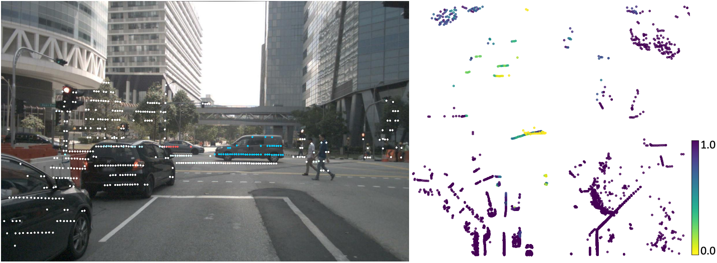
After factorizing out the ego-motion, we can use the object motion part of optical flow to approximate a probabilistic motion mask to indicate the probability of each pillar being static or dynamic. Specifically, the probability of each projected point being static can be computed by:
| (6) |
where is a smoothing factor and is a stationary tolerance. It is then back-projected to the point cloud coordinate, and we average of the points within a pillar to indicate the motion (being static) probability of this pillar, as shown in Figure 3. When the ego-vehicle (LiDAR) is moving, the scanned points even from background and static foreground objects cannot be exactly re-scanned over time. This introduces noise to the static regions when enforcing the nearest neighbor matching in the structural consistency loss, which treats all points equally. We can leverage the probabilistic motion mask to downweight the points from static pillars. In practice, we can simply enhance Eq. (1) by adding a weighting coefficient that is represented as the pillar motion probability for each point. Furthermore, since static pillars are often dominant in a scene, this weighting strategy also helps to balance the contributions of static and dynamic pillars in computing the overall structural consistency loss.
3.5 Optimization
Analogous to the spatial smoothness constraint for optical flow estimation, we also apply a local smoothness loss for pillar motion learning:
| (7) |
where and denote the and components of the predicted pillar motion field , and and are the gradients in and directions. Intuitively, this smoothness loss encourages the model to predict similar motion for the pillars belonging to the same object.
In summary, the total loss is a weighted sum of three terms including the probabilistic motion masking weighted structural consistency loss, the cross-sensor motion regularization loss, and the local smoothness loss:
| (8) |
where , and are the balancing coefficients to control the importance of the three loss terms. We train our model to jointly optimize the total loss function.
3.6 Backbone Network
Our proposed self-supervised learning framework is independent of the backbone network and can be generalized to various modified spatio-temporal networks [6, 43]. In order to make fair comparisons with the existing supervised methods, we adopt a similar backbone network as [39]. In details, we first employ a simple pillar feature encoder [16] that consists of a linear layer followed by batch normalization [13], ReLU [25] and a max pooling to convert a raw point cloud to a feature map representation in BEV. We then input the feature map to a U-Net with separated spatial and temporal convolutions as well as lateral connections between encoder and decoder.
| Mask | Static | Speed 5m/s | Speed 5m/s | Nonempty | Foreground | Moving | |||||||||
| Mean | Median | Mean | Median | Mean | Median | Mean | Median | Mean | Median | Mean | Median | ||||
| (a) | 0.3701 | 0.0063 | 0.5014 | 0.1352 | 1.9405 | 1.2760 | 0.3437 | 0.0081 | 0.5936 | 0.1139 | 0.7516 | 0.2359 | |||
| (b) | 0.0285 | 0.0002 | 0.3733 | 0.0719 | 4.2954 | 3.9788 | 0.0897 | 0.0020 | 0.7914 | 0.0656 | 1.1267 | 0.3948 | |||
| (c) | 0.1688 | 0.0389 | 0.4277 | 0.1694 | 1.7603 | 1.2021 | 0.3133 | 0.0062 | 0.5667 | 0.1017 | 0.7064 | 0.1980 | |||
| (d) | 0.0738 | 0.0038 | 0.4017 | 0.1214 | 1.9384 | 1.2931 | 0.1085 | 0.0007 | 0.5416 | 0.0767 | 0.8064 | 0.2279 | |||
| (e) | 0.0619 | 0.0004 | 0.3438 | 0.1196 | 1.7119 | 1.1438 | 0.0846 | 0.0001 | 0.4494 | 0.0507 | 0.5953 | 0.1612 | |||
4 Experiments
In this section, we first describe our experimental setup. A variety of ablation studies are then performed to understand the contribution of each individual design in our approach. We report comparisons to the state-of-the-art methods on the benchmark dataset. In the end, we provide in-depth analysis with qualitative visualization results.
4.1 Experimental Setup
Dataset. We extensively evaluate the proposed approach on a large-scale autonomous driving dataset: nuScenes [3]. It contains 850 scenes with annotations, and each scene is around 40s. Following the experimental protocol in MotionNet [39], we use 500 scenes for training, 100 scenes for validation and 250 scenes for testing. This dataset provides a full sensor suite including LiDAR, cameras, radars, IMU and GPS. We adopt LiDAR and all six cameras during training, and only use LiDAR for inference. The frequency of LiDAR and cameras are 20Hz and 10Hz, respectively. We can derive the ground truth motion from the original detection and tracking annotations provided by the dataset. Unless specified, we only use the motion labeling in the evaluation stage, while only using the raw sensor inputs and the calibration data in the training stage.
Implementation Details. We implement our model in PyTorch [27], and train the model on 8 GPUs with a batch size of 64. We train the model for 200 epochs in total, and set the initial learning rate to be 0.0001 and decay the learning rate by a factor of 0.9 in every 20 epochs. AdamW [21] is used as the optimizer. We emperically set and in Eq. (6), and , and in Eq. (8). We take the current sweep and past four sweeps as input, and transform the four sweeps from past to the current coordinate system through ego-motion compensation. Our model outputs the displacement for the next 0.5s as the predicted motion. We follow [39] to crop a point cloud in the range of , and set the pillar size to be for fair comparisons.
We adopt PWC-Net [33] as the optical flow estimation network considering its accuracy and efficiency. It is unsupervised trained on the training images of nuScenes with occlusion-aware photometric constancy and spatial smoothness losses [37]. We expect more advanced unsupervised methods such as [22, 36] would improve optical flow quality and benefit our pillar motion learning further.
Evaluation Metrics. Following MotionNet [39], we report the mean and median errors measured on the nonempty pillars, which are divided into three speed groups, i.e., static, slow (m/s) and fast (m/s). Additionally, we also evaluate on all nonempty pillars, all foreground object pillars, and all moving object pillars. The reason for evaluating on the different groups is that the static regions in a scene are the majority, which would overwhelm the prediction error if averaging over the whole scene.
4.2 Ablation Studies
Contribution of Individual Component. We first perform a variety of combination experiments to evaluate the contribution of each individual component in our design. As shown in Table 1, the base model (a) trained only with the structural consistency loss does not perform well for the static group. This is in accordance with our previous analysis. By using the cross-sensor motion regularization as the only supervision, model (b) achieves impressive result for the static group thanks to the accurate ego-motion factorization that enables our approach to reliably recover the static points from optical flow. However, the result of this model for the fast speed group is far inferior. This is not surprising since merely having the motion regularization in 2D camera image space is ambiguous and there exists numerous possible motion in 3D point cloud space that corresponds to the same 2D projection. Above limitations of the models (a, b) together demonstrate the necessity to have motion self-supervision in both 2D and 3D.
Although model (c) that directly combines the structural consistency and motion regularization performs well for the fast speed group, it is still not optimal for the static and slow speed groups, mainly due to the inconsistency between the two losses on the static and slow moving regions. By integrating the probabilistic motion masking into model (c), the full model (e) achieves significant improvements for static and slow speed groups. This is because by suppressing the plausible static pillars, the model can be less confused by the noisy motion caused by the moving ego-vehicle, and therefore can better focus on learning of the true object motion. We also experiment with model (d) that is trained only with the probabilistic motion masking enhanced structural consistency. Compared to model (a), the improvements on static and slow speed groups are obvious. However, it is still inferior to the full model (e), which further validates the efficacy of the cross-sensor motion regularization to provide the complementary motion supervision.
| Method | Static | Speed 5m/s | Speed 5m/s | ||||||
|---|---|---|---|---|---|---|---|---|---|
| 10m | 20m | 30m | 10m | 20m | 30m | 10m | 20m | 30m | |
| 0.2042 | 0.2296 | 0.3701 | 0.4343 | 0.4190 | 0.5014 | 1.7702 | 1.8729 | 1.9405 | |
| + | 0.1424 | 0.1602 | 0.1688 | 0.4001 | 0.4167 | 0.4277 | 1.7599 | 1.7576 | 1.7603 |
| Full Model | 0.1036 | 0.0857 | 0.0619 | 0.3348 | 0.3412 | 0.3438 | 1.6904 | 1.6998 | 1.7119 |
| Method | Static | Speed 5m/s | Speed 5m/s | Time | |||
|---|---|---|---|---|---|---|---|
| Mean | Median | Mean | Median | Mean | Median | ||
| FlowNet3D (pre-trained) [20] | 2.0514 | 0.0000 | 2.2058 | 0.3172 | 9.1923 | 8.4923 | 0.434s |
| HPLFlowNet (pre-trained) [11] | 2.2165 | 1.4925 | 1.5477 | 1.1269 | 5.9841 | 4.8553 | 0.352s |
| Ours (self-supervised) | 0.1620 | 0.0010 | 0.6972 | 0.1758 | 3.5504 | 2.0844 | 0.020s |
| FlowNet3D [20] | 0.0410 | 0.0000 | 0.8183 | 0.1782 | 8.5261 | 8.0230 | 0.434s |
| HPLFlowNet [11] | 0.0041 | 0.0002 | 0.4458 | 0.0969 | 4.3206 | 2.4881 | 0.352s |
| PointRCNN [31] | 0.0204 | 0.0000 | 0.5514 | 0.1627 | 3.9888 | 1.6252 | 0.201s |
| LSTMEncoderDecoder [30] | 0.0358 | 0.0000 | 0.3551 | 0.1044 | 1.5885 | 1.0003 | 0.042s |
| MotionNet [39] | 0.0239 | 0.0000 | 0.2467 | 0.0961 | 1.0109 | 0.6994 | 0.019s |
| MotionNet (pillar-based) [39] | 0.0258 | - | 0.2612 | - | 1.0747 | - | 0.019s |
| MotionNet+MGDA [39] | 0.0201 | 0.0000 | 0.2292 | 0.0952 | 0.9454 | 0.6180 | 0.019s |
| Ours (fine-tuned) | 0.0245 | 0.0000 | 0.2286 | 0.0930 | 0.7784 | 0.4685 | 0.020s |
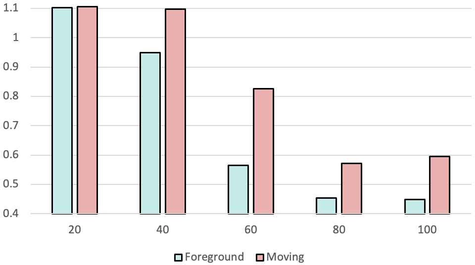
Amount of Training Data. Next we study how the amount of training data impacts our self-supervised learning. Since the foreground and moving objects are more concerned and challenging, we plot the mean errors of our full model on the two groups under different percentages of training data in Figure 4. With the increase of training size from to , our approach can boost the performance from to and to for the foreground and moving groups. Overall, more unlabeled training data leads to significantly better prediction results, suggesting the great potential of our self-supervised approach to harvest the vast amount of self-driving data that is available today.
Performance vs. Distance. Since the point clouds become more and more sparse with the increasing of distance, we also study how our model behaves at different ranges of LiDAR. As shown in Table 2, we compute the mean errors of each speed group within the distances of 10m, 20m and 30m, respectively. Specifically, the performance of our full model degrades , and from near to far regions in the three speed groups, as compared to the much larger performance drops of , and for the structural consistency only based model. Combining structural consistency and cross-sensor regularization also achieves apparent improvement over the base model. This verifies that optical flow provides more dense information complementary to point clouds and our full model regularized by optical flow is more robust to the distant pillars.
4.3 Comparison with State-of-the-Art Results
As reported in the ablation studies, our model is trained to predict the displacements for next 0.5s as the keyframes are sampled at 2Hz in nuScenes. Here for fair comparisons with the methods that evaluate for next 1.0s, we simply linearly interpolate our predicted displacements to 1.0s by assuming constant velocity in a short time frame.
We extensively compare our approach with a variety of supervised algorithms in Table 3. For our self-supervised model, we first compare to FlowNet3D and HPLFlowNet, which are pre-trained on FlyingThings3D and KITTI Scene Flow. As can be seen in this table, our model largely outperforms the two methods that are supervised pre-trained though. Remarkably, our self-supervised model is found to even outperform or approach some methods that are fully supervised trained on the benchmark dataset, for instance, our model performs better than FlowNet3D, HPLFlowNet and PointRCNN for the fast speed group. All these comparisons collectively and clearly show the advantage of our proposed self-supervisory design and the importance of self-supervised training on the target domain.
When further fine-tuning our self-supervised model with the ground truth labels, our approach achieves the state-of-the-art result. As we can see in Table 3, our fine-tuned model clearly outperforms the related methods of MotionNet for the fast moving objects. In particular, when compared to the strong MotionNet+MGDA, we perform better with a clear margin of mean error and median error for the fast speed group. This indicates that our self-supervised model provides a better foundation to allow for more effective supervised training, and the self-supervised learning gain does not diminish with the sophisticated supervised training design.
4.4 Runtime Analysis
At the inference stage, our whole model runs at 20ms on a single TITAN RTX GPU. In more details, the point cloud transformation and voxelization use 10ms, and the network forward time takes 10ms. As shown in Table 3, compared with the existing point cloud based motion estimation networks, our model is more computational efficient and is capable of dealing with large-scale point clouds in real time.
4.5 Qualitative Results
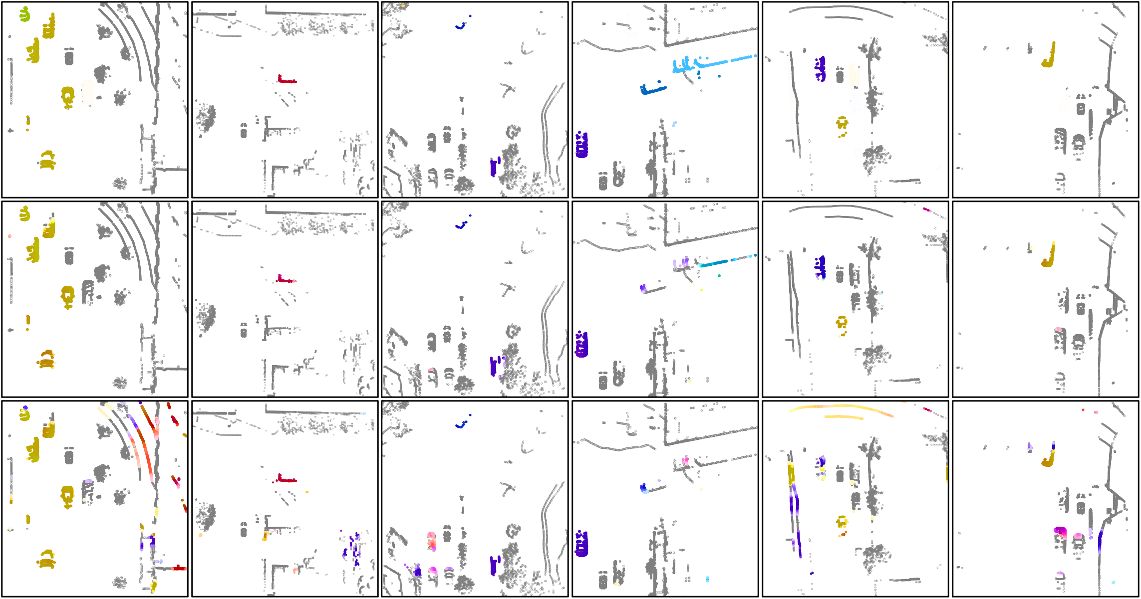
Finally, we demonstrate the qualitative results of pillar motion estimation using different combinations of the proposed self-supervised components. As shown in Figure 5, these examples present diverse traffic scenes and different zoom-in scales. In comparison to our full model, the base model using only structural consistency loss tends to generate false positive motion predictions in the background regions (columns 1 and 5) and static foreground objects (columns 2 and 3). This observation verifies our interpretation in Section 3.4 that the noise induced by the moving ego-vehicle is detrimental to the structural consistency matching when applied in the background and static foreground pillars. Our full model can successfully eliminate most false positive motion, indicating that the optical flow based regularization and masking are effective to suppress such noise. Compared to the base model, the full model is also able to produce spatially smoother motion on the moving objects (columns 5 and 6). Moreover, as illustrated in column 4, a moving truck on top right of the scene is missing in the base model, but it is reasonably well estimated by our full model. This again validates the efficacy of the distilled motion information from camera images.
5 Conclusion
In this paper, we propose a self-supervised learning framework for pillar motion estimation from unlabeled collections of point clouds and paired camera images. Our model involves a point cloud based structural consistency that is augmented with probabilistic motion masking and a cross-sensor motion regularization. Extensive experiments demonstrate that our self-supervised approach achieves superior or comparable results to the supervised methods, and outperforms the state-of-the-art methods when our model is further supervised fine-tuned. We hope these findings would encourage more research works on pillar motion estimation and point cloud based self-supervised learning.
Appendix
Appendix A Self-Supervision for Supervised Training
Our self-supervised learning can be utilized as unsupervised pre-training to improve supervised training. In this section, we investigate the benefits of our self-supervised pre-trained models to supervised training under different amounts of training data with the derived motion annotations. Specifically, we randomly sample 20%, 40%, 60% and 80% of the entire training data. We compare the models trained from scratch against the ones initialized from the self-supervised pre-trained models. Here we summarize the important findings from the comparisons reported in Table 4. (1) It is observed that the self-supervised pre-trained models consistently and significantly outperform the randomly initialized models across all cases. Such improvements are more remarkable under fewer training data and for the fast speed group. (2) Our self-supervised model fine-tuned with a small amount of training data (i.e., 20%) is able to achieve comparable performance compared to the randomly initialized model trained with a large amount of training data (i.e., 80%). This suggests that the model with self-supervised pre-training requires much fewer annotations and is therefore more labeling efficient. (3) We find that the self-supervised pre-trained models converge faster, taking about 60% of the training iterations as the models initialized from scratch.
Appendix B Pillar Motion for Downstream Tasks
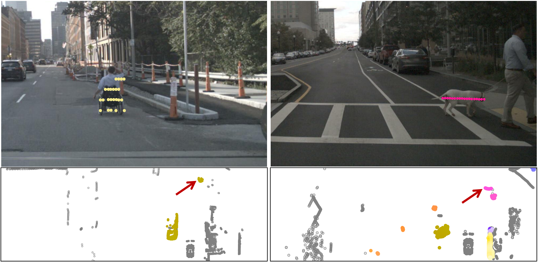
Our pillar motion can be potentially applied to enhance a variety of downstream modules. For perception, we show one advantage of our model to deal with the unknown instances that are not seen during the training of 3D object detection, as illustrated in Figure 6. For tracking, it is empirically demonstrated in [17] that integrating the low-level motion information improves the object tracking performance. As for planning, knowing the moving state of an agent is particularly helpful to tackle rare objects although the specific classes are unknown.
| Amount | Self-Supervised | Static | Speed 5m/s | Speed 5m/s | |||
| Mean | Median | Mean | Median | Mean | Median | ||
| 0% | ✓ | 0.1620 | 0.0010 | 0.6972 | 0.1758 | 3.5504 | 2.0844 |
| 20% | ✗ | 0.0473 | 0.0001 | 0.4635 | 0.1400 | 2.0946 | 1.1676 |
| ✓ | 0.0394 | 0.0001 | 0.2970 | 0.1309 | 1.028 | 0.6055 | |
| 40% | ✗ | 0.0459 | 0.0001 | 0.3712 | 0.1385 | 1.7060 | 0.8950 |
| ✓ | 0.0329 | 0.0000 | 0.2813 | 0.1280 | 0.8923 | 0.5287 | |
| 60% | ✗ | 0.0412 | 0.0001 | 0.3082 | 0.1338 | 1.0912 | 0.6830 |
| ✓ | 0.0352 | 0.0000 | 0.2801 | 0.1297 | 0.8499 | 0.5148 | |
| 80% | ✗ | 0.0347 | 0.0001 | 0.2930 | 0.1322 | 0.9824 | 0.6110 |
| ✓ | 0.0247 | 0.0000 | 0.2301 | 0.0933 | 0.7788 | 0.4700 | |
Appendix C Comparison with Scene Flow Estimation
In addition to the comparisons described in the introduction and related work of the paper, here we elaborate more on the differences between our work and the previous methods for point cloud based scene flow estimation. First, scene flow aims to estimate the point correspondences between two point clouds, while our goal is to predict the motion of each pillar or the displacement vector that indicates the future position of each pillar. Second, although apart from the synthetic data (e.g., FlyingThings3D), the existing scene flow methods also experiment with the self-driving data (e.g., KITTI Scene Flow), they do not use the raw LiDAR scans. Instead, they combine 2D optical flow with depth map and convert them into 3D scene flow. Compared with the point clouds collected by LiDAR, the converted point clouds are much more dense. However, for the raw point clouds used by self-driving vehicles, this does not hold in most cases, making the task harder, in particular for directly doing self-supervision. Third, the prior scene flow methods usually take hundreds of milliseconds when operating on a partial point cloud that is even largely subsampled. Our approach can achieve pillar motion prediction of a complete point cloud in real-time.
Appendix D Ablation Study on Smoothness
Removing the smoothness term in Eq. 8 slightly increases the mean errors, e.g., 0.0058 (Speed 5m/s), 0.0041 (Speed 5m/s), and 0.0042 (Moving). Overall, the smoothness loss in pillar motion is not as significant as in optical flow. This is due to the fact that the form of pillar motion representation already implies the smoothness prior as each pillar shares the same motion in . In addition, the motion prediction of empty pillars that occupy a large portion of areas can be directly masked out.
Appendix E Hyper-Parameters
We set the hyper-parameters to roughly balance the different loss terms: and . We also experiment with . Under the five values of , the standard deviations of mean errors of the three speed groups are very low: 0.0004, 0.0010 and 0.0070, indicating the robustness of our model to the hyper-parameter setting.
Appendix F More Qualitative Results
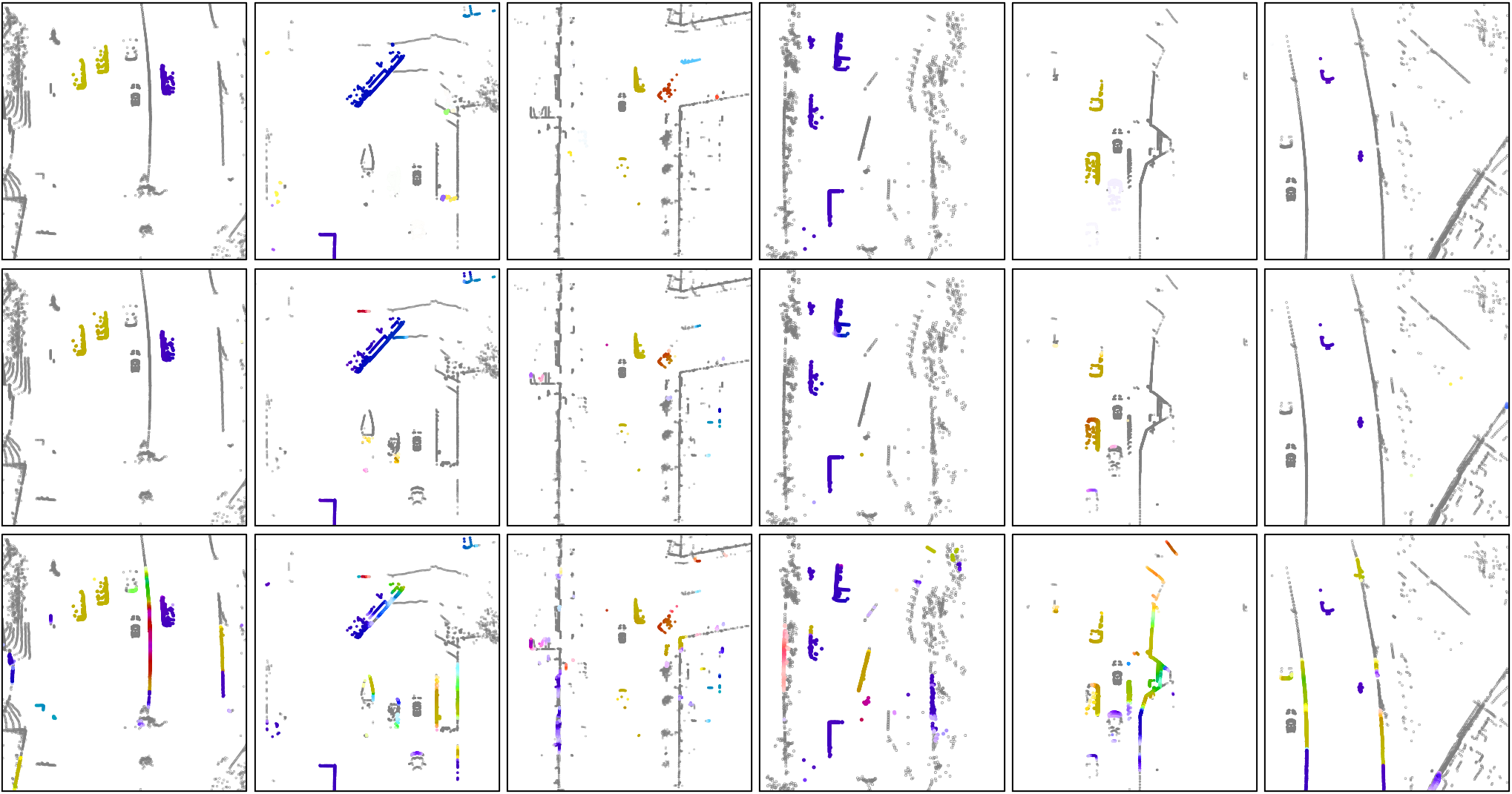
Next we provide more qualitative results to reveal the efficacy of the proposed probabilistic motion masking. In Figure 7, we compare the predicted pillar motion fields by our full model and the model without using probabilistic motion masking. As shown in this figure, we present 6 scenes with diverse traffic scenarios and multiple zoom-in scales. In comparison to our full model, the model not using probabilistic motion masking tends to produce more false positive motion predictions at the background regions, such as building, wall and vegetation. This comparison further validates the effect of probabilistic motion masking to reduce the noise incurred by the moving ego-vehicle to the pillars of the background regions.
References
- [1] https://www.siasearch.io/product.
- [2] Ramy Battrawy, Rene Schuster, Oliver Wasenmuller, Qing Rao, and Didier Stricker. LiDAR-Flow: Dense scene flow estimation from sparse LiDAR and stereo images. In IROS, 2019.
- [3] Holger Caesar, Varun Bankiti, Alex H. Lang, Sourabh Vora, Venice Erin Liong, Qiang Xu, Anush Krishnan, Yu Pan, Giancarlo Baldan, and Oscar Beijbom. nuScenes: A multimodal dataset for autonomous driving. In CVPR, 2020.
- [4] Xiaozhi Chen, Huimin Ma, Ji Wan, Bo Li, and Tian Xia. Multi-view 3D object detection network for autonomous driving. In CVPR, 2017.
- [5] Jacob Devlin, Ming-Wei Chang, Kenton Lee, and Kristina Toutanova. BERT: Pre-training of deep bidirectional Transformers for language understanding. In NAACL, 2019.
- [6] Christoph Feichtenhofer, Haoqi Fan, Jitendra Malik, and Kaiming He. SlowFast networks for video recognition. In ICCV, 2019.
- [7] Basura Fernando, Hakan Bilen, Efstratios Gavves, and Stephen Gould. Self-supervised video representation learning with odd-one-out networks. In CVPR, 2017.
- [8] Artem Filatov, Andrey Rykov, and Viacheslav Murashkin. Any motion detector: Learning class-agnostic scene dynamics from a sequence of LiDAR point clouds. In ICRA, 2020.
- [9] Jiyang Gao, Chen Sun, Hang Zhao, Yi Shen, Dragomir Anguelov, Congcong Li, and Cordelia Schmid. VectorNet: Encoding HD maps and agent dynamics from vectorized representation. In CVPR, 2020.
- [10] Andreas Geiger, Philip Lenz, and Raquel Urtasun. Are we ready for autonomous driving? The KITTI vision benchmark suite. In CVPR, 2012.
- [11] Xiuye Gu, Yijie Wang, Chongruo Wu, Yong-Jae Lee, and Panqu Wang. HPLFlowNet: Hierarchical permutohedral lattice FlowNet for scene flow estimation on large-scale point clouds. In CVPR, 2019.
- [12] Marcel Van Herk. Image registration using chamfer matching. Handbook of Medical Imaging, 2000.
- [13] Sergey Ioffe and Christian Szegedy. Batch normalization: Accelerating deep network training by reducing internal covariate shift. In ICML, 2015.
- [14] Longlong Jing, Xiaodong Yang, Jingen Liu, and Yingli Tian. Self-supervised spatiotemporal feature learning via video rotation prediction. arXiv:1811.11387, 2019.
- [15] Zhenzhong Lan, Mingda Chen, Sebastian Goodman, Kevin Gimpel, Piyush Sharma, and Radu Soricut. ALBERT: A lite BERT for self-supervised learning of language representations. In ICLR, 2020.
- [16] Alex H. Lang, Sourabh Vora, Holger Caesar, Lubing Zhou, Jiong Yang, and Oscar Beijbom. PointPillars: Fast encoders for object detection from point clouds. In CVPR, 2019.
- [17] Kuan-Hui Lee, Matthew Kliemann, Adrien Gaidon, Jie Li, Chao Fang, Sudeep Pillai, and Wolfram Burgard. PillarFlow: End-to-end birds-eye-view flow estimation for autonomous driving. In IROS, 2020.
- [18] Ming Liang, Bin Yang, Rui Hu, Yun Chen, Renjie Liao, Song Feng, and Raquel Urtasun. Learning lane graph representations for motion forecasting. In ECCV, 2020.
- [19] Ming Liang, Bin Yang, Shenlong Wang, and Raquel Urtasun. Deep continuous fusion for multi-sensor 3D object detection. In ECCV, 2018.
- [20] Xingyu Liu, Charles Qi, and Leonidas Guibas. FlowNet3D: Learning scene flow in 3D point clouds. In CVPR, 2019.
- [21] Ilya Loshchilov and Frank Hutter. Decoupled weight decay regularization. In ICLR, 2019.
- [22] Chenxu Luo, Zhenheng Yang, Peng Wang, Yang Wang, Wei Xu, Ram Nevatia, and Alan Yuille. Every pixel counts++: Joint learning of geometry and motion with 3D holistic understanding. TPAMI, 2019.
- [23] Nikolaus Mayer, Eddy Ilg, Philip Hausser, Philipp Fischer, Daniel Cremers, Alexey Dosovitskiy, and Thomas Brox. A large dataset to train convolutional networks for disparity, optical flow, and scene flow estimation. In CVPR, 2016.
- [24] Himangi Mittal, Brian Okorn, and David Held. Just go with the flow: Self-supervised scene flow estimation. In CVPR, 2020.
- [25] Vinod Nair and Geoffrey E. Hinton. Rectified linear units improve restricted Boltzmann machines. In ICML, 2010.
- [26] Simon Niklaus and Feng Liu. Context-aware synthesis for video frame interpolation. In CVPR, 2018.
- [27] Adam Paszke, Sam Gross, Francisco Massa, Adam Lerer, James Bradbury, Gregory Chanan, Trevor Killeen, Zeming Lin, Natalia Gimelshein, Luca Antiga, et al. PyTorch: An imperative style, high-performance deep learning library. In NeurIPS, 2019.
- [28] Charles Qi, Wei Liu, Chenxia Wu, Hao Su, and Leonidas Guibas. Frustum PointNets for 3D object detection from RGB-D data. In CVPR, 2018.
- [29] Rishav, Ramy Battrawy, Rene Schuster, Oliver Wasenmuller, and Didier Stricker. DeepLiDARFlow: A deep learning architecture for scene flow estimation using monocular camera and sparse LiDAR. In IROS, 2020.
- [30] Marcel Schreiber, Stefan Hoermann, and Klaus Dietmayer. Long-term occupancy grid prediction using recurrent neural networks. In ICRA, 2019.
- [31] Shaoshuai Shi, Xiaogang Wang, and Hongsheng Li. PointRCNN: 3D object proposal generation and detection from point cloud. In CVPR, 2019.
- [32] Deqing Sun, Xiaodong Yang, Ming-Yu Liu, and Jan Kautz. PWC-Net: CNNs for optical flow using pyramid, warping and cost volume. In CVPR, 2018.
- [33] Deqing Sun, Xiaodong Yang, Ming-Yu Liu, and Jan Kautz. Models matter, so does training: An empirical study of CNNs for optical flow estimation. TPAMI, 2019.
- [34] Carl Vondrick, Abhinav Shrivastava, Alireza Fathi, Sergio Guadarrama, and Kevin Murphy. Tracking emerges by colorizing videos. In ECCV, 2018.
- [35] Sourabh Vora, Alex H. Lang, Bassam Helou, and Oscar Beijbom. PointPainting: Sequential fusion for 3D object detection. In CVPR, 2020.
- [36] Yang Wang, Peng Wang, Zhenheng Yang, Chenxu Luo, Yi Yang, and Wei Xu. UnOS: Unified unsupervised optical-flow and stereo-depth estimation by watching videos. In CVPR, 2019.
- [37] Yang Wang, Yi Yang, Zhenheng Yang, Liang Zhao, Peng Wang, and Wei Xu. Occlusion aware unsupervised learning of optical flow. In CVPR, 2018.
- [38] Kelvin Wong, Shenlong Wang, Mengye Ren, Ming Liang, and Raquel Urtasun. Identifying unknown instances for autonomous driving. In CoRL, 2019.
- [39] Pengxiang Wu, Siheng Chen, and Dimitris Metaxas. MotionNet: Joint perception and motion prediction for autonomous driving based on bird’s eye view maps. In CVPR, 2020.
- [40] Wenxuan Wu, Zhiyuan Wang, Zhuwen Li, Wei Liu, and Fuxin Li. PointPWC-Net: Cost volume on point clouds for (self-)supervised scene flow estimation. In ECCV, 2020.
- [41] Saining Xie, Jiatao Gu, Demi Guo, Charles Qi, Leonidas Guibas, and Or Litany. PointContrast: Unsupervised pre-training for 3D point cloud understanding. In ECCV, 2020.
- [42] Xiaodong Yang, Pavlo Molchanov, and Jan Kautz. Making convolutional networks recurrent for visual sequence learning. In CVPR, 2018.
- [43] Xitong Yang, Xiaodong Yang, Ming-Yu Liu, Fanyi Xiao, Larry Davis, and Jan Kautz. STEP: Spatio-temporal progressive learning for video action detection. In CVPR, 2019.
- [44] Xitong Yang, Xiaodong Yang, Sifei Liu, Deqing Sun, Larry Davis, and Jan Kautz. Hierarchical contrastive motion learning for video action recognition. arXiv:2007.10321, 2020.
- [45] Yuting Zhang, Yijie Guo, Yixin Jin, Yijun Luo, Zhiyuan He, and Honglak Lee. Unsupervised discovery of object landmarks as structural representations. In CVPR, 2018.