Question Decomposition with Dependency Graphs
Abstract
QDMR is a meaning representation for complex questions, which decomposes questions into a sequence of atomic steps. While state-of-the-art QDMR parsers use the common sequence-to-sequence (seq2seq) approach, a QDMR structure fundamentally describes labeled relations between spans in the input question, and thus dependency-based approaches seem appropriate for this task. In this work, we present a QDMR parser that is based on dependency graphs (DGs), where nodes in the graph are words and edges describe logical relations that correspond to the different computation steps. We propose (a) a non-autoregressive graph parser, where all graph edges are computed simultaneously, and (b) a seq2seq parser that uses gold graph as auxiliary supervision. We find that a graph parser leads to a moderate reduction in performance (0.470.44), but to a 16x speed-up in inference time due to the non-autoregressive nature of the parser, and to improved sample complexity compared to a seq2seq model. Second, a seq2seq model trained with auxiliary graph supervision has better generalization to new domains compared to a seq2seq model, and also performs better on questions with long sequences of computation steps.
1 Introduction
Training neural networks to reason over multiple parts of their inputs across modalities such as text, tables, and images, has been a focal point of interest in recent years Antol et al. (2015); Pasupat and Liang (2015); Johnson et al. (2017); Suhr et al. (2019); Welbl et al. (2018); Talmor and Berant (2018); Yang et al. (2018); Hudson and Manning (2019); Dua et al. (2019); Chen et al. (2020); Hannan et al. (2020); Talmor et al. (2021). The most common way to check whether a model is capable of complex reasoning, is to pose in natural language a complex question, which requires performing multiple steps of computation over the input.
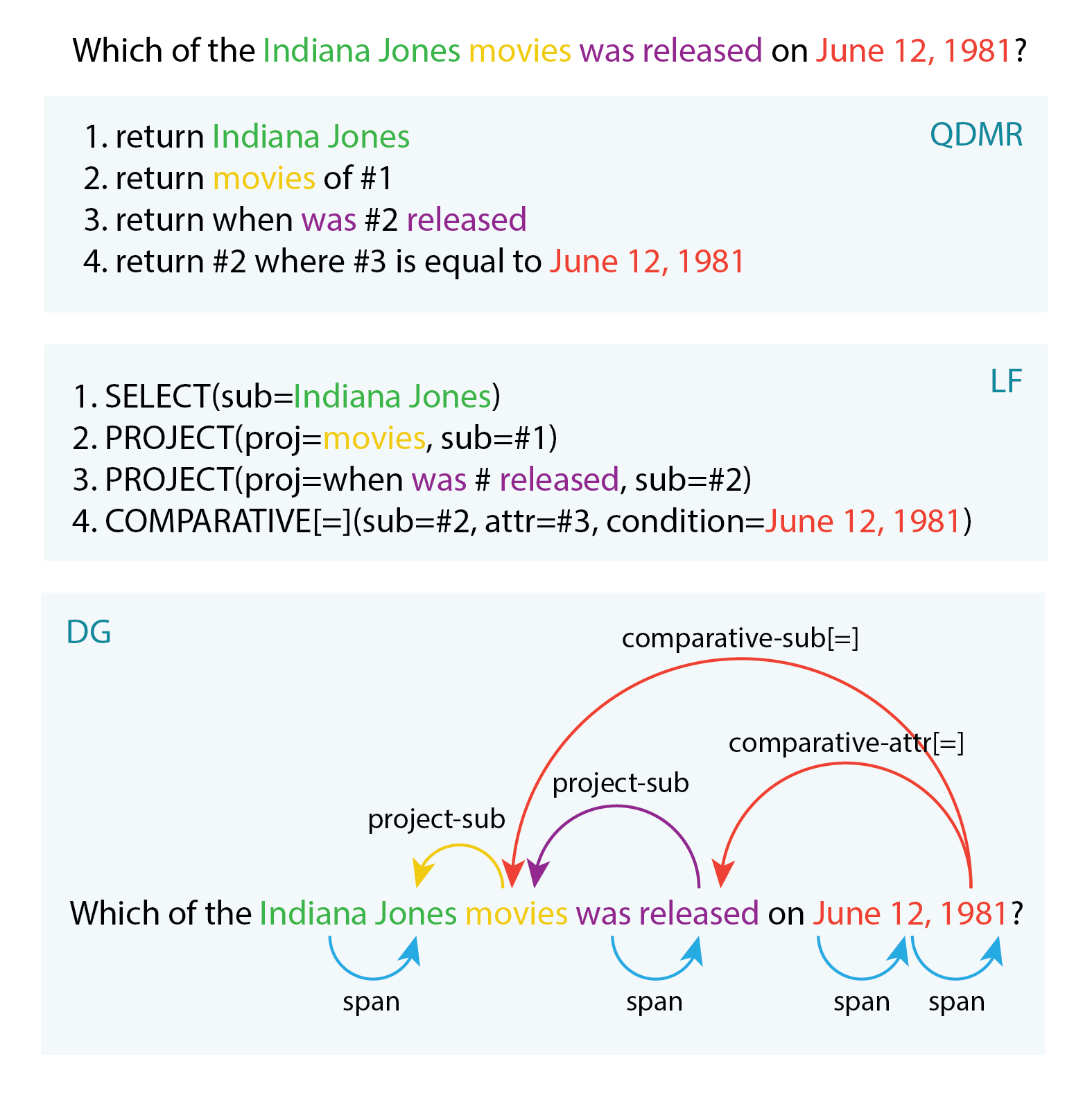
To address the need for better understanding of complex questions, Wolfson et al. (2020) recently proposed QDMR, a meaning representation where complex questions are represented through a sequence of simpler atomic executable steps (see Fig. 1), and the final answer is the answer to the final step. QDMR has been shown to be useful for multi-hop question answering (QA) Wolfson et al. (2020) and also for improving interpretability in visual QA Subramanian et al. (2020).
State-of-the-art QDMR parsers use the typical sequence-to-sequence (seq2seq) approach. However, it is natural to think of QDMR as a dependency graph over the input question tokens. Consider the example in Fig. 1. The first QDMR step selects the span “Indiana Jones”. Then, the next step uses a PROJECT operation to find the “movies” of Indiana Jones, and then next step uses another PROJECT operation to find the date when the movies were “released”. Such relations can naturally be represented as labeled edges over the relevant question tokens, as shown in Fig. 1, bottom.
In this work, we propose to use the dependency graph view of QDMR to improve QDMR parsing. We describe a conversion procedure that automatically maps QDMR structures into dependency graphs, using a structured intermediate logical form representation (Fig 1, middle). Once we have graph supervision for every example, we train a dependency graph parser, in the spirit of Dozat and Manning (2018), where we predict a labeled relation for every pair of question tokens, representing the logical relation between the tokens. Unlike seq2seq models, this is a non-autoregressive parser, which decodes the entire output structure in a single step.
A second method to exploit the graph supervision is to train a seq2seq model, but have an auxiliary loss term where the graph is decoded from the encoder representations. Towards that end, we propose a Latent-RAT encoder, which uses relation-aware transformer Shaw et al. (2018) to explicitly represent the relation between every pair of input tokens. Relation-aware transformer has been shown to be useful for encoding graph structures in the context of semantic parsing Wang et al. (2020).
Last, we propose a new evaluation metric, LF-EM, for QDMR parsing, which is based on the aforementioned intermediate logical form, and show it correlates better with human judgements compared to existing metrics.
We find that our graph parser leads to a small reduction in LF-EM compared to seq2seq models (0.470.44), but is 16x faster due to its non-autoregressive nature. Moreover, our graph parser has better sample complexity and outperforms the seq2seq model when trained on 10% of the data or less. When training a seq2seq model along with the auxiliary graph supervision, we find that the parser obtains similar performance when trained on the entire dataset (0.471 LF-EM), but substantially improves performance when generalizing to new domains. Moreover, The Latent-RAT parser performs better on examples with a large number of computation steps.
Our code is available at https://github.com/matanhasson/qdecomp_with_dependency_graphs.
2 Overview
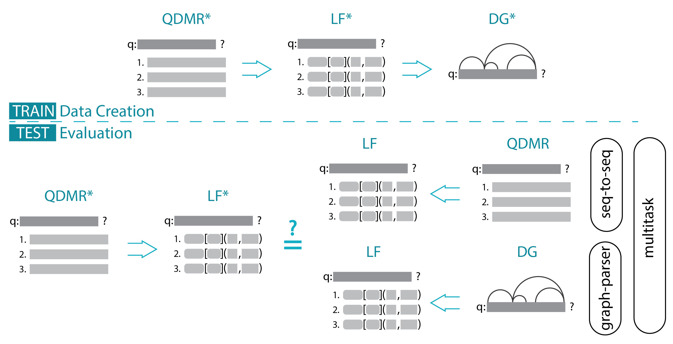
The core of this work is to examine the utility of a dependency graph (DG) representation for QDMR. We propose conversion procedures that enable training and evaluating with DGs (see Fig. 2). First, we convert gold QDMR structures into logical forms (LF), where each computation step in QDMR is represented with a formal operator, properties and arguments (§3.1). Then, we obtain gold DGs by projecting the logical forms onto the question tokens (§4). Once we have question-DG pairs, we can train a graph parser. At test time, QDMRs and DGs are converted into LFs for evaluation. We propose a new evaluation metric over LFs (§3.2), and show it is more robust to semantic-preserving changes compared to prior metrics.
Our proposed parsers are in §5. On top of standard seq2seq models, we describe (a) a graph parser, and (b) a multi-task model, where the encoder of the seq2seq model is also trained to predict the DG.
3 QDMR Logical Forms
QDMR Wolfson et al. (2020) is a text-based meaning representation focused on representing the meaning of complex questions. It is based on a decomposition of questions into a sequence of simpler executable steps (Fig. 1), where each step corresponds to a SQL-inspired operator (Table 6 in Appendix §A.1). We briefly review QDMR and then define a logical form (LF) representation based on these operations. We use the LFs both for mapping QDMRs to DGs, and also to fairly evaluate the output of parsers that output either QDMRs directly or DGs.
3.1 Definitions
QDMR Definition
Given a question with tokens, , its QDMR is a sequence of steps , where step conceptually maps to a single logical operator . A step, , is a sequence of tokens , where token is either a question token (or some inflection of it), a word from a constant predefined lexicon , or a reference token , referring to a previous step. Fig. 3 shows an example for a question and its QDMR structure.
“Which group from the census is smaller: Pacific islander or African American?”
1. return census groups
2. return #1 that is Pacific islander
3. return #1 that is African American
4. return size of #2
5. return size of #3
6. return which is lowest of #4 , #5
QDMR Logical Form (LF)
Given a QDMR , its logical form is a sequence of logical form steps . The LF step , corresponding to , is a triplet where is the logical operator; are operator-specific properties; and is a dictionary of arguments, mapping an operator-specific argument to a span from the QDMR step . For convenience, we denote with the string . Table 1 provides a few examples for the mapping from QDMR to LF steps, and Table 6 in the Appendix provides the full list.
Imposing more structure on QDMR through the LF is useful (a) for evaluation (§3.2), where LFs detect differenet QDMR phrasings that have identical meaning, and (b) for creating DGs, since the operators, properties and arguments, will be used to define the labels of edges in the DG (see Fig 1).
| Operator | PROP | ARG | Example |
| SELECT | sub | return cubes | |
| SELECT[](sub=cubes) | |||
| FILTER | sub, cond | return #1 from Toronto | |
| FILTER[](sub=#1, cond=from Toronto) | |||
| AGGREGATE | max, min, count, sum, avg | arg | return maximal number of #1 |
| AGGREGATE[max]( | |||
| arg=#1) | |||
| ARITHMETIC | sum, diff, mult, div | arg, left, right | return the difference of #3 and #4 |
| ARITHMETIC[diff]( | |||
| left=#3, right=#4) |
QDMRLF
3.2 LF-based Evaluation (LF-EM)
The official evaluation metric for QDMR111https://leaderboard.allenai.org/break/submissions/public is normalized EM (NormEM), where the predicted and gold QDMR structures are normalized using a rule-based procedure, and then exact string match is computed between the two normalized QDMRs. Since in this work we convert both QDMRs (§3.1) and DGs (§4) to LFs, we propose LF-EM, a LF-based evaluation metric, and show that it correlates better with notions of semantic equivalence.
LF-EM essentially involves computing exact match between the predicted and gold LFs, using the LF described above. To further capture semantic equivalences, we perform a few more normalization steps. We briefly describe these normalizations, and give the full description in §A.2.
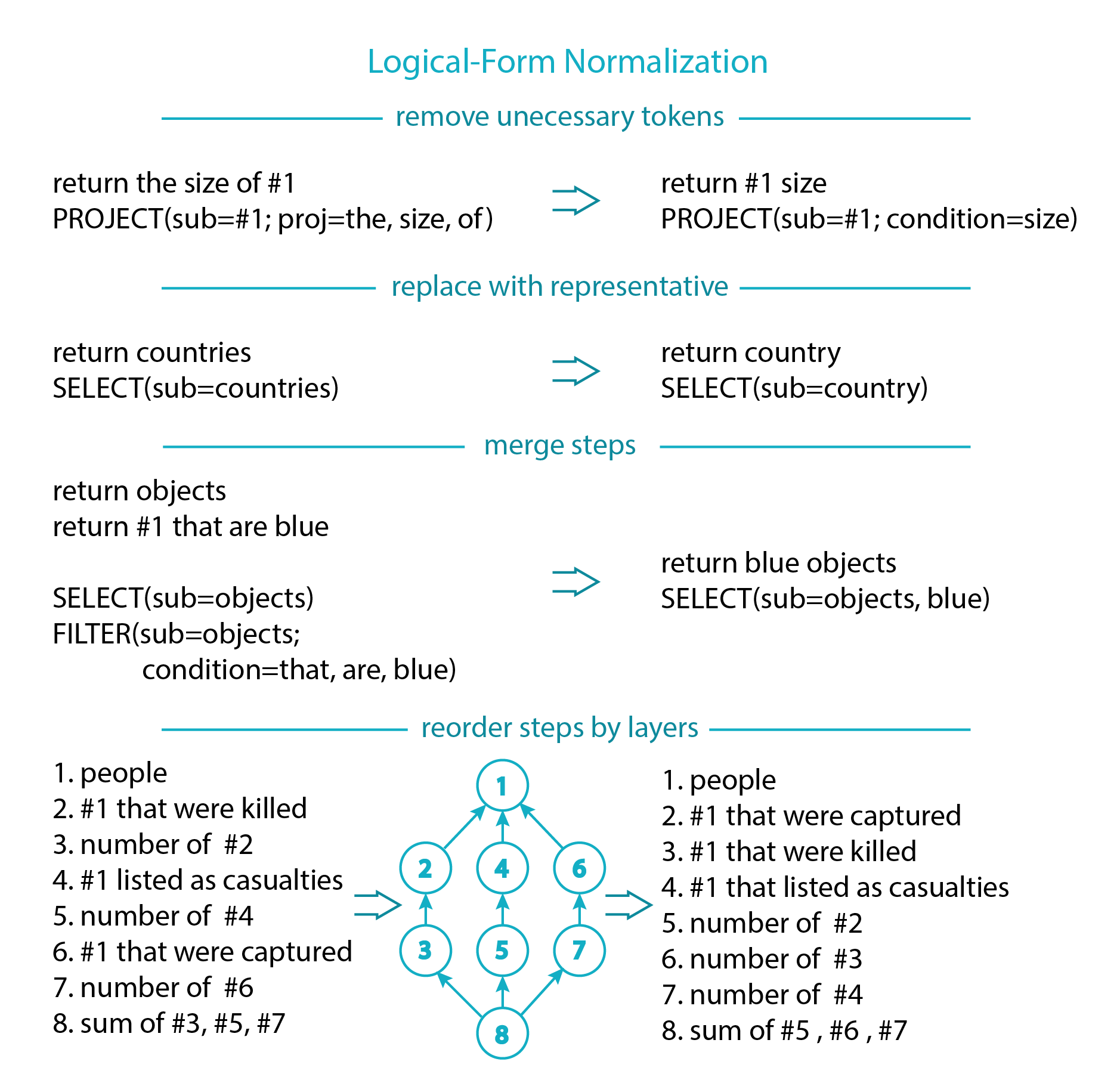
Given a logical form , we transform each step to a normalized form, and the final textual representation is given by representing each step as described in §3: OPERATOR[property](arg=…; …). We apply the following steps (Fig. 4):
Remove and normalize tokens
Each LF step includes a list of tokens in its arguments. In this normalization step, we remove lexical items, such as “max”, which are used to detect the operator and property (Table 7 in §A.1), as those are already represented outside the arguments. In addition, we remove words from a stop word list (, see Fig. 3). Finally, we use a synonym list to represent words in such a list with a single representative (countriescountry).
Merge Steps
QDMR annotations sometime vary in their granularity. For example one example might contain ‘return metal objects’, while another might have ‘return objects; return #1 that are metal’. This is especially common in FILTER and PROJECT steps. We merge chains of FILTER steps, as well as FILTER or PROJECT steps that follow a SELECT step. See details in §A.2.
Reorder steps
QDMR describes a directed acyclic graph of computation steps, and there are multiply ways to order the steps (Fig. 4). We recursively compute the layer of each step as , where the maximization is over all steps refers to. We then re-order steps by layer and then lexicographically.
We manually evaluate the metrics normalized EM and LF-EM on 50 random development set examples using predictions from the CopyNet-BERT model (see §6). We find that both (binary) metrics have perfect precision: they only assign credit when indeed the QDMR reflects the correct question decomposition, as judged by the authors. However, LF-EM covers more examples, where the LF-EM on this sample is 52.0, while normalized EM is 40.0. Thus, LF-EM provides a tighter lower bound on the performance of a QDMR parser and is a better metric for QDMR parsing.
4 From LFs to Dependency Graphs
Given a QDMR decomposition , we construct a dependency graph , where the nodes correspond to question tokens, and the edges describe the logical operations, resulting in a graph with the same meaning as .
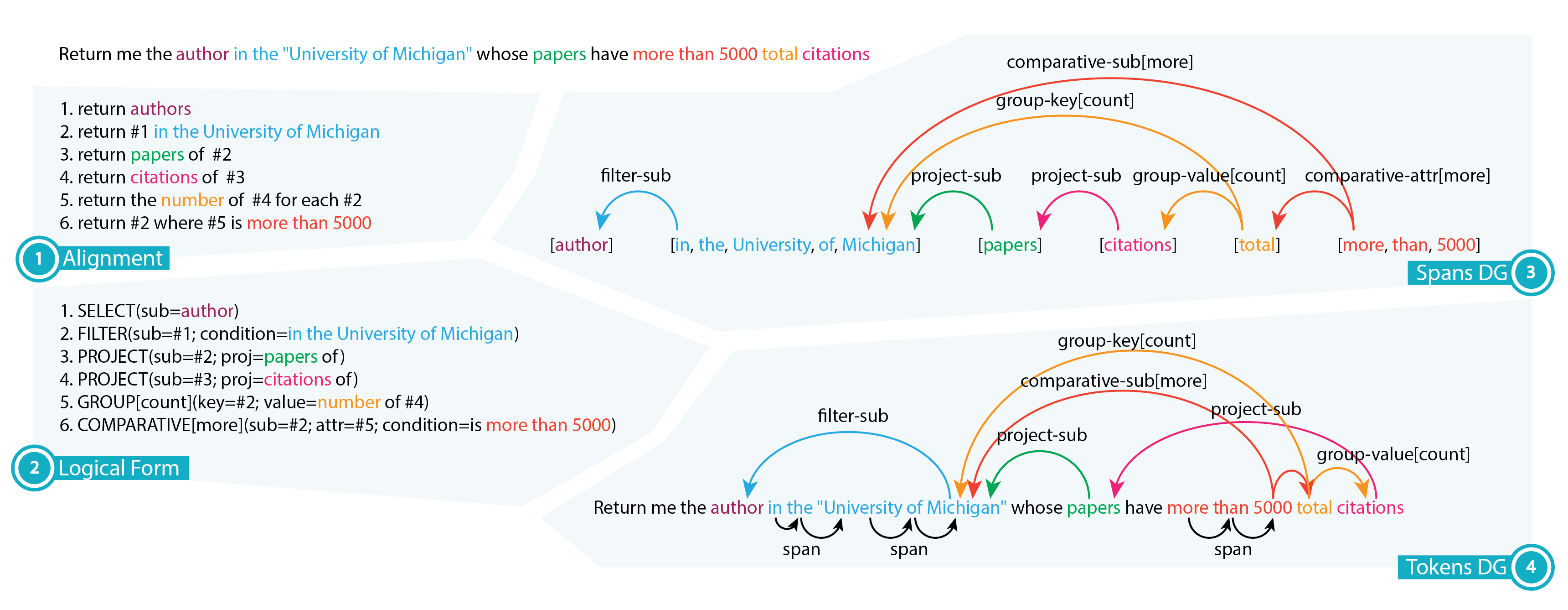
The LFDG procedure is shown in Fig. 5 and consists of the following steps:
-
•
Token alignment: align each token in the question to a token in a QDMR step.
-
•
Spans Dependency Graph (SDG) extraction: construct a graph where each node corresponds to a list of tokens in a QDMR step, and edges describe the dependencies between the steps.
-
•
Dependency Graph (DG) extraction: convert the SDG to a DG over the question tokens. Here, we add span edges for tokens that are in the same step, and deal with some representation issues (see §4.3).
Because we convert predicted DGs to LFs for evaluation, the LFDG conversion must be invertible. We now describe the details of the LFDG conversion. Our conversion succeeds in 97.12% of the BREAK dataset Wolfson et al. (2020).
4.1 Token Alignment
We denote the question tokens by and the th QDMR step tokens by . An alignment is defined by , where by we mean are either identical or equivalent. Roughly speaking, these equivalences are based on BREAK annotation lexicon (Fig. 3) - in particular. the inflections of the question tokens (e.g , “object” and “objects”), and equivalence classes on top of the constant lexicon (e.g , “biggest” and “longest”). See Table 8 in Appendix §A.2 for more details.
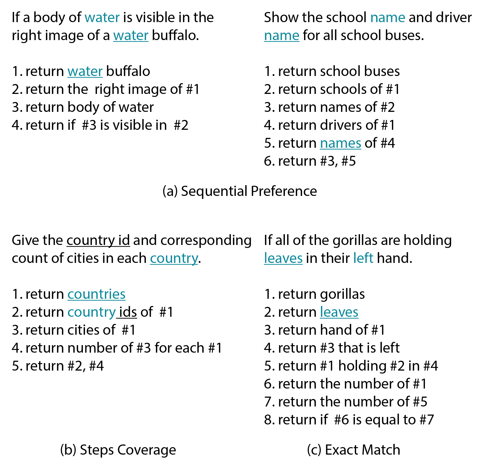
To find the best alignment , we formulate an optimization problem in the form of an Integer Linear Program (ILP) and use a standard ILP solver.222https://developers.google.com/optimization The full details are given as a part of our open source implementation. The objective function uses several heuristics to assign a high score to an alignment the has the following properties (Fig. 6):
-
•
Minimalism: Aligning each question token to at most one QDMR step token and vice versa is preferable.
-
•
Exact Match: Aligning a question token to a QDMR token that is identical is preferable.
-
•
Sequential Preference: Aligning long sequences from the question to a single step is preferable (when a step has a reference token (#1), we take into account the tokens in the referenced step, see Fig. 6, top right).
-
•
Steps Coverage: Covering more steps is preferable.
4.2 Spans Dependencies Extraction
Given the QDMR, LF, and alignment , we construct the Span Dependency Graph (SDG). Each QDMR step is a node labeled by a list of tokens (spans). The list of tokens is computed with the alignment , where given a QDMR step , the list contains all question tokens , such that , where is a word in . The list is ordered according to the position in the question.
Edges in the SDG are computed using reference tokens. If step has a reference token to step , we add an edge (we abuse notation and refer to SDG nodes and QDMR steps with the same notation). Each edge has a tag, which is a triple consisting of the operator of the source node , the property of the source node, and the named argument that contains the reference token. For readability we denote the tag triplet by -. Figure 5 shows an extracted SDG.
4.3 SDGDG
We construct a DG by projecting the SDG on the question tokens. This is done by: (a) For each SDG node and its list of tokens, add edges between the tokens from left-to-right with a new span tag (black edges in Fig 5); (b) use the rightmost word in every span as its representative for the edges between different spans.
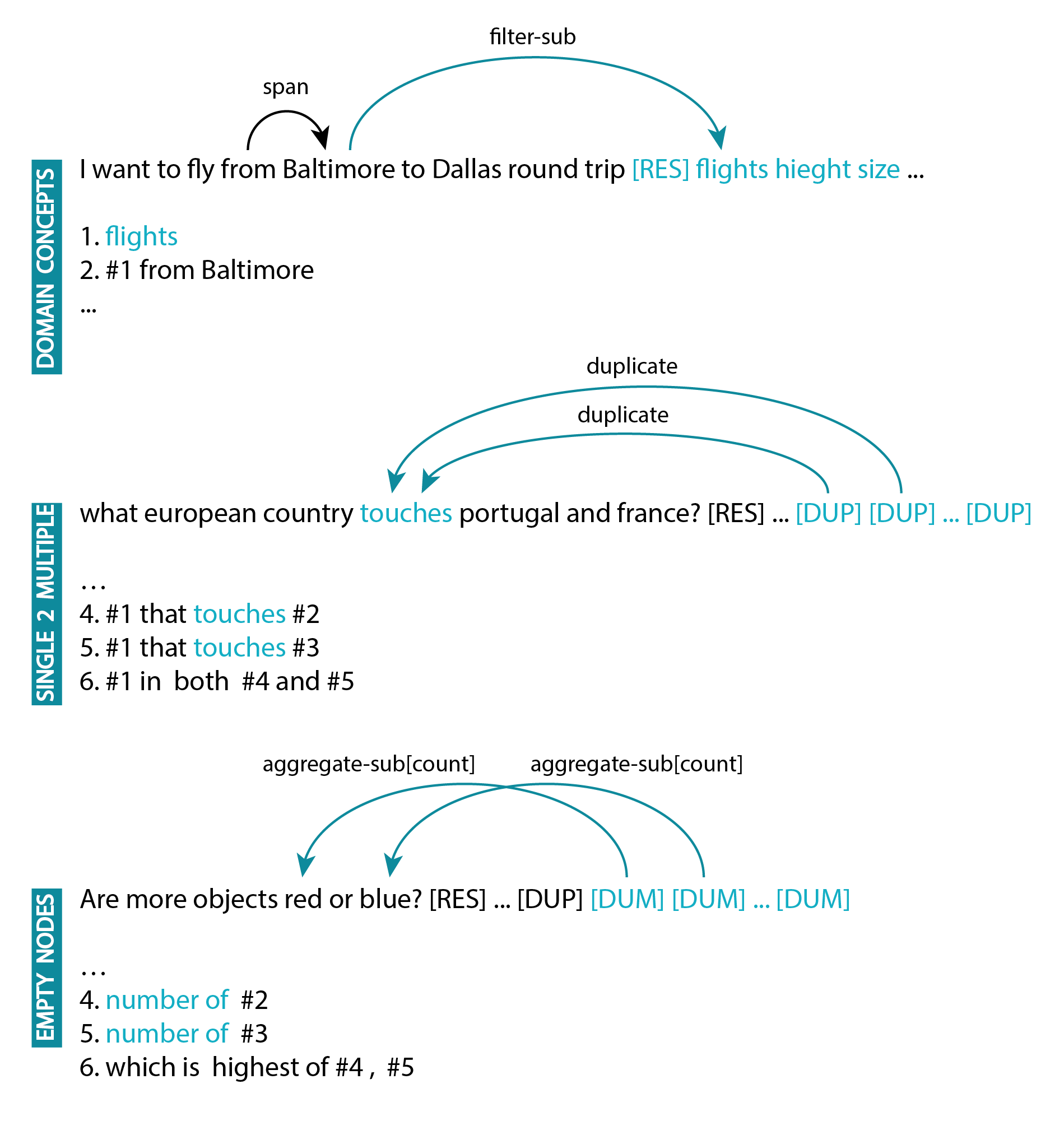
However, this transformation is non-trivial for two reasons. First, some SDG nodes do not align to any question token, Second, some question tokens align to multiple SDG nodes, which does not allow the DG to be converted back to an SDG unambiguously for evaluation. We now explain how we resolve such representation issues, mostly based on adding more tokens to the input question. Fig. 7 illustrates the different types of challenges and our proposed solution.
Domain-specific concepts
QDMR annotators were allowed to use a small number of tokens that are pragmatically assumed to exist in the domain ( in Fig. 3). For example, when annotating ATIS questions Hemphill et al. (1990), the word “flight” is allowed to be used in the QDMR structure even if it does not appear in the question, since this is a flight-reservation domain. We concatenate all the words in to the end of each question after a special separator token, which allows token alignment (§4.1) to map such QDMR steps to a question word (Fig. 7, top).
Empty SDG nodes
some steps only contains tokens that are not in the question (e.g, “Number of #2” in Fig. 7 bottom), and thus their list of tokens in the SDG node is empty. In this case, we cannot ground the SDG node in the question. Therefore we add a constant number of dummy tokens, [DUM], which are used to ground such SDG nodes.
Single tokens to multiple SDG nodes
A single question token can be aligned to multiple SDG nodes. Recall the tokens of each SDG nodes are connected with a chain of span edges. This leads to cases where two chains that pass through the same question token cannot be distinguished when converting the DG back to an SDG for evaluation. We solve this by concatenating a constant number of special [DUP] tokens that conceptually duplicate another token by referring to it with a new duplicate tag. Now, each span chain uses a different copy of the shared token by referring to the [DUP] instead of the original one.
5 Models
Once we have methods to convert QDMRs to DGs and LFs, and DGs to LFs, we can evaluate the advantages and disadvantages of standard autoregressive decoders compared to graph-based parsers. We describe three models: (a) An autoregressive parser, (b) a graph parser, (c) an autoregressive parser that is trained jointly with a graph parser in a multi-task setup. For a fair comparison, all models have the same BERT-based encoder Devlin et al. (2019).
CopyNet-BERT (baseline)
This autoregressive QDMR parser is based on the CopyNet baseline from Wolfson et al. (2020), except we replace the BiLSTM encoder with a transformer initialized with BERT. The model encodes the question and then decodes the QDMR step-by-step and token-by-token.
The QDMR decoder is an LSTM Hochreiter and Schmidhuber (1997) augmented with a copy mechanism Gu et al. (2016), where at each time step the model either decodes a token from the vocabulary or a token from the input. Since the input is tokenized with word pieces, we average word pieces that belong to a single word to get word representations, which enables word copying. Training is dones with standard maximum likelihood.
Biaffine Graph Parser (BiaffineGP)
The biaffine graph parser takes as input the quesiton augmented with the special tokens described in §4.3 and predicts the DG by classifying for every pair of tokens whether there is an edge between them and the label of the edge. The model is based on the biaffine dependency parser of Dozat and Manning (2018), except here we predict a DAG and not a tree, so each node can have more that one outgoing edge.
Let be the sequence of representations output by the BERT encoder. The biaffine parser uses four 1-hidden layer feed-forward networks over each contextualized token representation :
The probability of an edge from token to token is given by , where is a parameter matrix. Similarly, the score of an edge labeled by the tag from token to token is given by , where is the parameter matrix for this tag. We then compute a distribution over the set of tags with .
Training is done with maximum likelihood both on the edge probabilities and label probabilities. Inference is done by taking all edges with edge probability and then labeling those edges according to the most probable tag.
There is no guarantee that the biaffine parser will output a valid DG. For example, if an SDG node has an outgoing edge labeled with filter-sub and another labeled with project-sub, we cannot tell if the operator is FILTER or PROJECT. This makes parsing fail, which occurs in 1.83% of the cases. To create a SDG, we first use the span edges to contruct SDG nodes with lists of tokens, and then add edges between SDG nodes by projecting the edges between tokens to edges between the SDG nodes. To prevent cases where parsing fails, we can optionally apply an ILP that takes the predicted probabilities as input, and outputs a valid DG. The exact details are given in our open source implementation.
Multi-task Latent-RAT Encoder
In this model, our goal is to improve the sequence-to-sequence parser by providing more information to the encoder using the DG supervision. Our model will take the question (with special tokens as before) as input, and predict both the graph directly and the QDMR structure with a decoder.
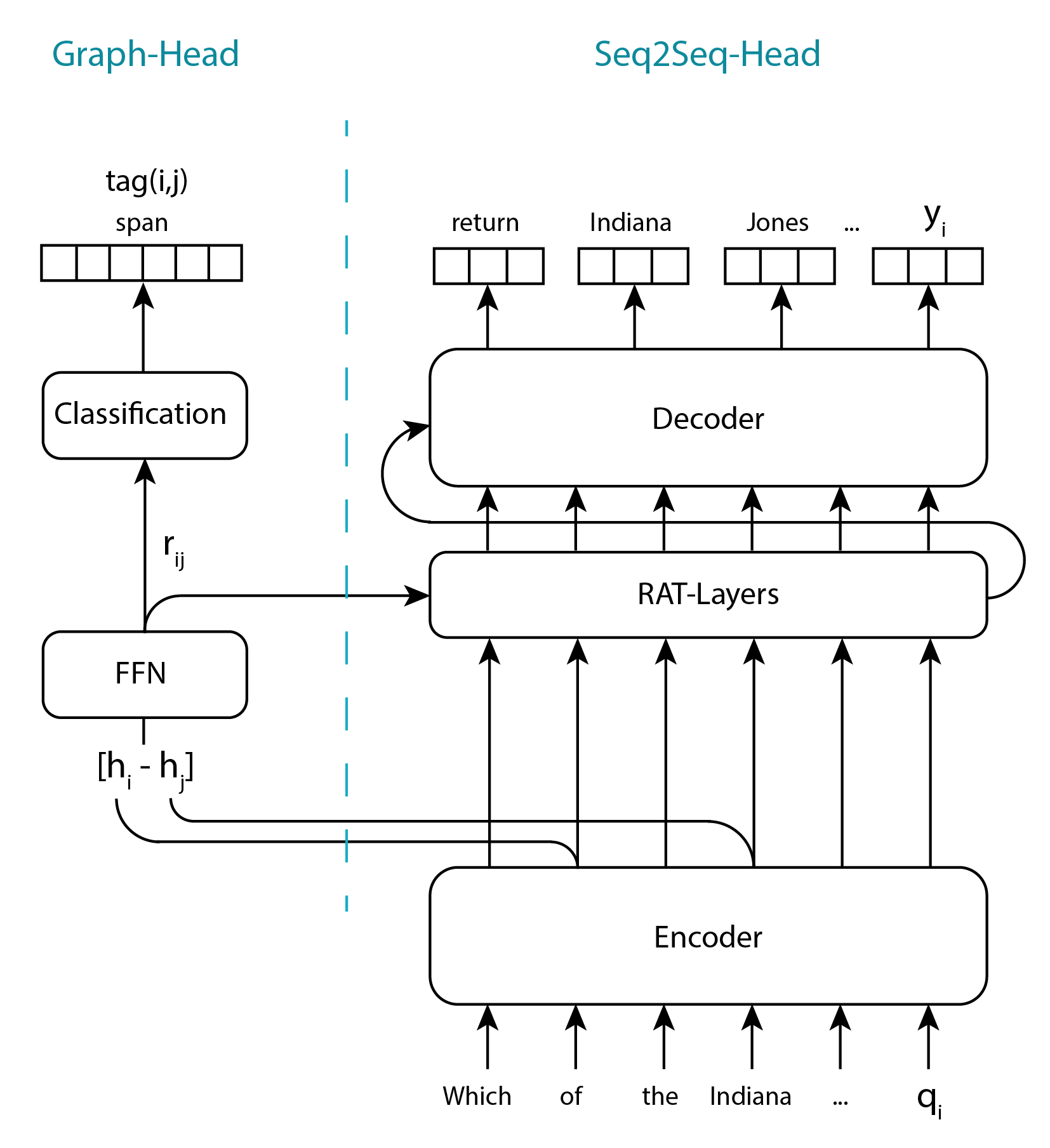
We would like the information on relations between tokens to be part of the transformer encoder, unlike the biaffine parser that uses separate feed-forward networks for that, so that the decoder can take advantage of this information. To accomplish that, we use RAT transformer layers Shaw et al. (2018); Wang et al. (2020), which explicitly represent relations between tokens, and have been shown to be useful for encoding graphs over input tokens in the context of semantic parsing.
RAT layers inject information on the relation between tokens inside the transformer self-attention mechanism Vaswani et al. (2017). Specifically, the similarity score computed using queries and keys is given by:
where are the query and key parameter matrices and the only change is the term , which represents the relation between the tokens and . Similarly, the relation between tokens is also considered when summing over self-attention values:
where is the value parameter matrix, is the attention distribution and the only change is the term .
Unlike prior work where the terms were learned parameters, here we want these vectors to (a) be a function of the contextualized representation and (b) be informative for classifying the dependency label in the gold graph. By learning latent representations from which the gold graph can be decoded, we will provide useful information for the sequence-to-sequence decoder. Specifically, given a RAT layer with representations for tokens and , we represent relations and compute a loss in the following way (see Figure 8):
is a 1-hidden layer feed-forward network, is a concatenation of all for all pairs of tokens, is a projection matrix that provides a score for all possible labels (including the NONE label).
We compute an analogous loss for and the final graph loss is over all RAT layers. To summarize, by performing multi-task training with this graph loss we push the transformer to learn representations that are informative of the gold graph, and can then be used by the decoder to output better QDMR structures.
6 Experiments
We now describe our empirical evaluation of the models described above.
6.1 Experimental Setup
We build our models in AllenNLP Gardner et al. (2018), and use BERT-base Devlin et al. (2019) to produce contextualized token representations in all models. We train with the Adam optimizer Kingma and Ba (2015). Our Latent-RAT model include 4 RAT layers, each with 8 heads. Full details on hyperparameters and training procedure in Appendix §A.3.
We examine the performance of our models in three setups:
-
•
Standard: We use the official BREAK dataset.
-
•
Sample Complexity (SC): We examine the performance of models with decreasing amounts of training data. The goal is to test which model has better sample complexity.
-
•
Domain Generalization (DomGen): We train on 7 out of 8 sub-domains in BREAK and test on the remaining domain, for each target domain. The goal is to test which model generalizes better to new domains.
As an evaluation metric, we use LF-EM and also the official BREAK metric, normalized EM, when reporting test results on BREAK.
6.2 Results
Standard setup
Table 2 compares the performance of the different models (§5) to each other and to the top entries on the BREAK leaderboard. As expected, initializing CopyNet with BERT dramatically improves test performance (0.3880.47). The Latent-RAT sequence-to-sequence model achieves similar performance (0.471), and the biaffine graph parser, BiaffineGP, is slightly behind with an LF-EM of 0.44 (but has faster inference, as we show below). Adding an ILP layer on top of BiaffineGP to eliminate constraint violations in the output graph improves performance to 0.454.
While our proposed models do not significantly improve performance in the LF-EM setup, we will see next that they improve domain generalization and sample complexity. Moreover, since BiaffineGP is a non-autoregressive model that predicts all output edges simultaneously, it dramatically reduces inference time.
Last, the top entry on the BREAK leaderboard uses BART Lewis et al. (2020), a pre-trained seq2seq model (we use a pre-trained encoder only), which leads to a state-of-the-art LF-EM of 0.496.
| Model | NormEM | LF-EM | ||
| dev | test | dev | test | |
| CopyNet | - | 0.294 | - | 0.388 |
| BART | - | 0.389 | - | 0.496 |
| CopyNet+BERT | 0.373 | 0.375 | 0.474 | 0.47 |
| BiaffineGP | - | - | 0.441 | 0.44 |
| BiaffineGP | - | - | 0.453 | 0.454 |
| Latent-RAT | 0.356 | 0.363 | 0.469 | 0.471 |
Domain generalization
Table 3 shows LF-EM on each of BREAK’s sub-domains when training on the entire dataset (top), when training on all domains but the target domain (middle), and the relative drop compared to the standard setup (bottom).
The performance of BiaffineGP and Latent-RAT is higher compared to CopyNET+BERT in the DomGen setup. In particular, the performance of Latent-RAT is the best in 7 out of 8 sub-domains, and the performance of BiaffineGP is the best in the last domain. Moreover, Latent-RAT outperforms CopyNet+BERT in all sub-domains. We also observe that the performance drop is lower for BiaffineGP and Latent-RAT compared to CopyNet+BERT. Overall, this shows that using graphs as a source of supervision leads to better domain generalization.
| Model | ATIS | CLEVR | COMQA | CWQ | DROP | GEO | NLVR2 | SPIDER |
|---|---|---|---|---|---|---|---|---|
| CopyNet+BERT | 0.58 | 0.564 | 0.562 | 0.36 | 0.473 | 0.66 | 0.344 | 0.369 |
| BiaffineGP | 0.591 | 0.489 | 0.595 | 0.322 | 0.445 | 0.62 | 0.293 | 0.41 |
| Latent-RAT | 0.589 | 0.524 | 0.598 | 0.316 | 0.479 | 0.64 | 0.353 | 0.376 |
| CopyNet+BERT | 0.282 | 0.351 | 0.423 | 0.173 | 0.131 | 0.52 | 0.039 | 0.189 |
| BiaffineGP | 0.302 | 0.339 | 0.483 | 0.168 | 0.146 | 0.52 | 0.04 | 0.197 |
| Latent-RAT | 0.335 | 0.356 | 0.435 | 0.189 | 0.149 | 0.58 | 0.063 | 0.201 |
| CopyNet+BERT | -51.38% | -37.77% | -24.73% | -51.94% | -72.30% | -21.21% | -88.66% | -48.78% |
| BiaffineGP | -48.90% | -30.67% | -18.82% | -47.83% | -67.19% | -16.13% | -86.35% | -51.95% |
| Latent-RAT | -43.12% | -32.06% | -27.26% | -40.19% | -68.89% | -9.38% | -82.15% | -46.54% |
Sample Complexity
Table 4 shows model performance as a function of the size of the training data. While the LF-EM of BiaffineGP is lower given the full training set (Table 2), when the size of the training data is small it substantially outperforms other models, improving performance by 3-4 LF-EM points given 1%-10% of the data. With 20%-50% of the data Latent-RAT and CopyNet+BERT have comparable performance.
| Model | 1% | 5% | 10% | 20% | 50% |
|---|---|---|---|---|---|
| CopyNet | 0.112 | 0.261 | 0.323 | 0.38 | 0.426 |
| BiaffineGP | 0.159 | 0.296 | 0.351 | 0.382 | 0.411 |
| Latent-RAT | 0.003 | 0.227 | 0.326 | 0.383 | 0.432 |
Inference time for the graph parser
The graph parser, BiaffineGP, is a non-autoregressive model that predicts all output edges simultaneously, as opposed to a sequence-to-sequence model that decodes a single token at each step. We measure the average runtime of the forward pass for both BiaffineGP and CopyNet+BERT and find that BiaffineGP has an average runtime of 0.08 seconds, compared to 1.306 seconds of CopyNet+BERT – a 16x speed-up.
6.3 Analysis
Model agreement
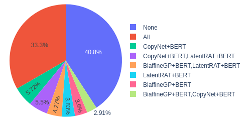
Figure 9 shows model agreement between CopyNet+BERT, BiaffineGP, and Latent-RAT on the development set. Roughly 60% of the examples are predicted correctly by one of the models, indicating that enembling the three models could result in further performance improvement.
The agreement of Latent-RAT with CopyNet+BERT (5.5%) and BiaffineGP (4.27%) is greather than the overlap between CopyNet+BERT and BiaffineGP, perhaps since it is a hybrid of a seq2seq and graph parser. Moreover, in 3.83% of the examples, Latent-RAT is the only model with a correct prediction.
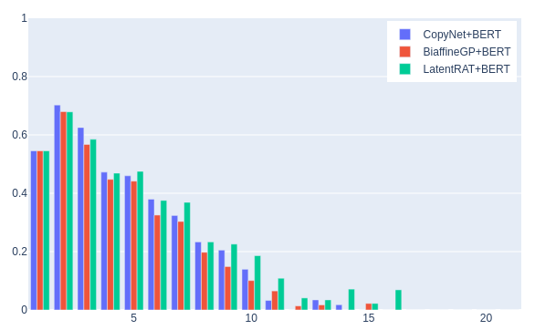
Length analysis
We compared the average LF-EM of models for each possible number of steps in the QDMR structure (Fig. 10). We observe that CopyNet+BERT outperforms Latent-RAT when the number of steps is small, but once the number of steps is , Latent-RAT outperforms CopyNet+BERT, showing it is handles complex decompositions better, and in agreement with the tendency of sequence-to-sequence models to struggle with long output sequences.
Error analysis
We randomly sampled 30 errors from each model and manually analyzed them. Table 5 describes the error classes for each model, and Appendix A.4 provides examples for these classes. Each example can have more than one error cateogry.
For all models, the largest error category is actually cases where the prediction is correct but not captured by the LF-EM metric: 70% for CopyNet+BERT, 40% for BiaffineGP and 73.3% for Latent-RAT. This shows that the performance of current QDMR parsers is actually quite good, but capturing this with an automatic evaluation is challenging. Cases where the output is correct include:
-
•
Equivalent Solutions: the prediction is logically equivalent to the gold structure.
-
•
Elaboration Level: the model prediction is more/less granular compared to the gold structure, but the prediction is correct.
-
•
Redundancy: additional information is predicted/omitted that does not effect the computation. For example the second occurrence of “yard’s’ in , ”2. return yards of #1; 3. #1 where #2 is lower than 10 yards”.
-
•
Wrong Gold - cases where the predication is more accurate than the gold decomposition.
The main classes of errors are:
-
•
Missing Information: missing steps, missing references or missing tokens that affect the result of the computation.
-
•
Additional Steps: duplicate steps or additional steps that change the result of the computation.
-
•
Wrong Global Structure: The computation described by the predicted structure is wrong (for example, addition instead of subtraction).
-
•
Wrong Step Structure: incoherent structure of a particular step that cannot be mapped to a proper structure.
-
•
Out of Vocabulary: seq2seq models sometimes predict tokens that are not related to the question nor the decomposition. For example, ”rodents” in a question about flowers.
| CopyN | BiaGP | LatRAT | |
| Correct | 70.00% | 40.00% | 73.30% |
| Equivalent Solutions | 40.00% | 30.00% | 43.30% |
| Elaboration Level | 26.70% | 23.30% | 26.70% |
| Redundancy | 10.00% | 0.00% | 3.30% |
| Wrong Gold | 0.00% | 3.30% | 3.30% |
| Missing Information | 16.70% | 20.00% | 10.00% |
| Additional Steps | 6.70% | 23.30% | 6.70% |
| Wrong Global Structure | 3.30% | 16.70% | 13.30% |
| Wrong Step Structure | 0.00% | 16.70% | 6.70% |
| Out of Vocab | 13.30% | 0.00% | 0.00% |
7 Conclusion
In this work, we propose to represent QDMR structures with a dependency graph over the input tokens, and propose a graph parser and a seq2seq model that uses graph supervision as an auxiliary loss. We show that a graph parser is 16x faster than a seq2seq model, and that it exhibits better sample coplexity. Moreover, using graphs as auxiliary supervision improves out-of-domain generalization and leads to better performance on questions that represent a long sequence of computational steps. Last, we propose a new evaluation metric for QDMR parsing and show it better corresponds to human intuitions.
In future work, we will examine ensemble models that take into account the complementary nature of graph parsers and seq2seq parser to further improve performance on QDMR parsing.
Acknowledgments
We thank Vivek Kumar Singh for his helpful ILP guidelines, and Tomer Wolfson for having kindly assisted in running our evaluation metric on our predictions for BREAK test set. This research was partially supported by The Yandex Initiative for Machine Learning, and the European Research Council (ERC) under the European Union Horizons 2020 research and innovation programme (grant ERC DELPHI 802800).
References
- Antol et al. (2015) Stanislaw Antol, Aishwarya Agrawal, Jiasen Lu, Margaret Mitchell, Dhruv Batra, C. Lawrence Zitnick, and Devi Parikh. 2015. VQA: visual question answering. In 2015 IEEE International Conference on Computer Vision, ICCV 2015, Santiago, Chile, December 7-13, 2015, pages 2425–2433. IEEE Computer Society.
- Chen et al. (2020) Wenhu Chen, Hanwen Zha, Zhiyu Chen, Wenhan Xiong, Hong Wang, and William Yang Wang. 2020. HybridQA: A dataset of multi-hop question answering over tabular and textual data. In Findings of the Association for Computational Linguistics: EMNLP 2020, pages 1026–1036, Online. Association for Computational Linguistics.
- Devlin et al. (2019) Jacob Devlin, Ming-Wei Chang, Kenton Lee, and Kristina Toutanova. 2019. BERT: Pre-training of deep bidirectional transformers for language understanding. In Proceedings of the 2019 Conference of the North American Chapter of the Association for Computational Linguistics: Human Language Technologies, Volume 1 (Long and Short Papers), pages 4171–4186, Minneapolis, Minnesota. Association for Computational Linguistics.
- Dozat and Manning (2018) Timothy Dozat and Christopher D. Manning. 2018. Simpler but more accurate semantic dependency parsing. In Proceedings of the 56th Annual Meeting of the Association for Computational Linguistics (Volume 2: Short Papers), pages 484–490, Melbourne, Australia. Association for Computational Linguistics.
- Dua et al. (2019) Dheeru Dua, Yizhong Wang, Pradeep Dasigi, Gabriel Stanovsky, Sameer Singh, and Matt Gardner. 2019. DROP: A reading comprehension benchmark requiring discrete reasoning over paragraphs. In Proceedings of the 2019 Conference of the North American Chapter of the Association for Computational Linguistics: Human Language Technologies, Volume 1 (Long and Short Papers), pages 2368–2378, Minneapolis, Minnesota. Association for Computational Linguistics.
- Gardner et al. (2018) Matt Gardner, Joel Grus, Mark Neumann, Oyvind Tafjord, Pradeep Dasigi, Nelson F. Liu, Matthew Peters, Michael Schmitz, and Luke Zettlemoyer. 2018. AllenNLP: A deep semantic natural language processing platform. In Proceedings of Workshop for NLP Open Source Software (NLP-OSS), pages 1–6, Melbourne, Australia. Association for Computational Linguistics.
- Gu et al. (2016) Jiatao Gu, Zhengdong Lu, Hang Li, and Victor O.K. Li. 2016. Incorporating copying mechanism in sequence-to-sequence learning. In Proceedings of the 54th Annual Meeting of the Association for Computational Linguistics (Volume 1: Long Papers), pages 1631–1640, Berlin, Germany. Association for Computational Linguistics.
- Hannan et al. (2020) Darryl Hannan, Akshay Jain, and Mohit Bansal. 2020. Manymodalqa: Modality disambiguation and QA over diverse inputs. In The Thirty-Fourth AAAI Conference on Artificial Intelligence, AAAI 2020, The Thirty-Second Innovative Applications of Artificial Intelligence Conference, IAAI 2020, The Tenth AAAI Symposium on Educational Advances in Artificial Intelligence, EAAI 2020, New York, NY, USA, February 7-12, 2020, pages 7879–7886. AAAI Press.
- Hemphill et al. (1990) Charles T. Hemphill, John J. Godfrey, and George R. Doddington. 1990. The ATIS spoken language systems pilot corpus. In Speech and Natural Language: Proceedings of a Workshop Held at Hidden Valley, Pennsylvania, June 24-27,1990.
- Hochreiter and Schmidhuber (1997) Sepp Hochreiter and Jürgen Schmidhuber. 1997. Long short-term memory. Neural computation, 9(8):1735–1780.
- Hudson and Manning (2019) Drew A. Hudson and Christopher D. Manning. 2019. GQA: A new dataset for real-world visual reasoning and compositional question answering. In IEEE Conference on Computer Vision and Pattern Recognition, CVPR 2019, Long Beach, CA, USA, June 16-20, 2019, pages 6700–6709. Computer Vision Foundation / IEEE.
- Johnson et al. (2017) Justin Johnson, Bharath Hariharan, Laurens van der Maaten, Li Fei-Fei, C. Lawrence Zitnick, and Ross B. Girshick. 2017. CLEVR: A diagnostic dataset for compositional language and elementary visual reasoning. In 2017 IEEE Conference on Computer Vision and Pattern Recognition, CVPR 2017, Honolulu, HI, USA, July 21-26, 2017, pages 1988–1997. IEEE Computer Society.
- Kingma and Ba (2015) Diederik P. Kingma and Jimmy Ba. 2015. Adam: A method for stochastic optimization. In 3rd International Conference on Learning Representations, ICLR 2015, San Diego, CA, USA, May 7-9, 2015, Conference Track Proceedings.
- Lewis et al. (2020) Mike Lewis, Yinhan Liu, Naman Goyal, Marjan Ghazvininejad, Abdelrahman Mohamed, Omer Levy, Veselin Stoyanov, and Luke Zettlemoyer. 2020. BART: Denoising sequence-to-sequence pre-training for natural language generation, translation, and comprehension. In Proceedings of the 58th Annual Meeting of the Association for Computational Linguistics, pages 7871–7880, Online. Association for Computational Linguistics.
- Pasupat and Liang (2015) Panupong Pasupat and Percy Liang. 2015. Compositional semantic parsing on semi-structured tables. In Proceedings of the 53rd Annual Meeting of the Association for Computational Linguistics and the 7th International Joint Conference on Natural Language Processing (Volume 1: Long Papers), pages 1470–1480, Beijing, China. Association for Computational Linguistics.
- Shaw et al. (2018) Peter Shaw, Jakob Uszkoreit, and Ashish Vaswani. 2018. Self-attention with relative position representations. In Proceedings of the 2018 Conference of the North American Chapter of the Association for Computational Linguistics: Human Language Technologies, Volume 2 (Short Papers), pages 464–468, New Orleans, Louisiana. Association for Computational Linguistics.
- Subramanian et al. (2020) Sanjay Subramanian, Ben Bogin, Nitish Gupta, Tomer Wolfson, Sameer Singh, Jonathan Berant, and Matt Gardner. 2020. Achieving interpretability in compositional neural networks. In Association for Computational Linguistics (ACL).
- Suhr et al. (2019) Alane Suhr, Stephanie Zhou, Ally Zhang, Iris Zhang, Huajun Bai, and Yoav Artzi. 2019. A corpus for reasoning about natural language grounded in photographs. In Proceedings of the 57th Annual Meeting of the Association for Computational Linguistics, pages 6418–6428, Florence, Italy. Association for Computational Linguistics.
- Talmor and Berant (2018) Alon Talmor and Jonathan Berant. 2018. The web as a knowledge-base for answering complex questions. In Proceedings of the 2018 Conference of the North American Chapter of the Association for Computational Linguistics: Human Language Technologies, Volume 1 (Long Papers), pages 641–651, New Orleans, Louisiana. Association for Computational Linguistics.
- Talmor et al. (2021) Alon Talmor, Ori Yoran, Amnon Catav, Dan Lahav, Yizhong Wang, Akari Asai, Gabriel Ilharco, Hannaneh Hajishirzi, and Jonathan Berant. 2021. Multimodalqa: Complex question answering over text, tables and images. In International Conference on Learning Representations (ICLR).
- Vaswani et al. (2017) Ashish Vaswani, Noam Shazeer, Niki Parmar, Jakob Uszkoreit, Llion Jones, Aidan N. Gomez, Lukasz Kaiser, and Illia Polosukhin. 2017. Attention is all you need. In Advances in Neural Information Processing Systems 30: Annual Conference on Neural Information Processing Systems 2017, December 4-9, 2017, Long Beach, CA, USA, pages 5998–6008.
- Wang et al. (2020) Bailin Wang, Richard Shin, Xiaodong Liu, Oleksandr Polozov, and Matthew Richardson. 2020. RAT-SQL: Relation-aware schema encoding and linking for text-to-SQL parsers. In Proceedings of the 58th Annual Meeting of the Association for Computational Linguistics, pages 7567–7578, Online. Association for Computational Linguistics.
- Welbl et al. (2018) Johannes Welbl, Pontus Stenetorp, and Sebastian Riedel. 2018. Constructing datasets for multi-hop reading comprehension across documents. Transactions of the Association for Computational Linguistics, 6:287–302.
- Wolfson et al. (2020) Tomer Wolfson, Mor Geva, Ankit Gupta, Matt Gardner, Yoav Goldberg, Daniel Deutch, and Jonathan Berant. 2020. Break it down: A question understanding benchmark. Transactions of the Association for Computational Linguistics, 8:183–198.
- Yang et al. (2018) Zhilin Yang, Peng Qi, Saizheng Zhang, Yoshua Bengio, William Cohen, Ruslan Salakhutdinov, and Christopher D. Manning. 2018. HotpotQA: A dataset for diverse, explainable multi-hop question answering. In Proceedings of the 2018 Conference on Empirical Methods in Natural Language Processing, pages 2369–2380, Brussels, Belgium. Association for Computational Linguistics.
Appendix A Appendices
A.1 QDMR LF
Table 6 shows the different operators, their properties and examples of LFs. Table 7 shows terms that are used to identify the QDMR step operator’s properties. We use the same lexicon from BREAK Wolfson et al. (2020) for detecting operators, extended with some specifications for numeric properties such as equals_0.
| Operator | PROP | ARG | Example |
|---|---|---|---|
| SELECT | sub | return cubes | |
| SELECT[](sub=cubes) | |||
| FILTER | sub, condition | return #1 from Toronto | |
| FILTER[](sub=#1, cond=from Toronto) | |||
| PROJECT | sub, projection | return the head coach of #1 | |
| PROJECT[](sub=#1, projection=the head coach of) | |||
| AGGREGATE | max, min, count, sum, avg | arg | return maximal number of #1 |
| AGGREGATE[max](arg=#1) | |||
| GROUP | max, min, count, sum, avg | key, value | return the number of #2 for each #1 |
| GROUP[count](key=#1, value=#2) | |||
| SUPERLATIVE | max, min | sub, attribute | return #2 where #3 is the lowest |
| SUPERLATIVE[min](sub=#2, attribute=#3) | |||
| COMPARATIVE | equals, equals-[0/1/2], more, more-than-[0/1/2], less, less-than-[0/1/2] | sub, attribute, condition | return #1 where #2 is more than 100 |
| COMPARATIVE[more](sub=#1, attribute=#2, condition=100) | |||
| COMPARISON | max, min, count, sum, avg, true, false | arg | return which is higher of #1, #2 |
| COMPARISON[max](arg=#1, arg=#2) | |||
| UNION | sub | return #1, #2 | |
| UNION[](sub=#1, sub=#2) | |||
| INTERSECTION | intersect, projection | return parties in both #2 and #3 | |
| INTERSECTION[](intersect=#2, intersect=#3, projection=parties) | |||
| DISCARD | sub, exclude | return #1 besides #2 | |
| DISCARD[](sub=#1, exclude=#2) | |||
| SORT | sub, order | return #1 ordered by name | |
| SORT[](sub=#2, order=name) | |||
| BOOLEAN | equals, equals-[0/1/2], more-than-[0/1/2], less-than-[0/1/2], and-true, and-false, or-true, or-false, if-exists | sub, condition | return if #1 is the same as #2 |
| BOOLEAN[equals](sub=#1, condition=#2) | |||
| ARITHMETIC | sum, diff, multiply, div | arg, left, right | return the difference of #3 and #4 |
| ARITHMETIC[diff](left=#3, right=#4) |
| Operator | PROP | Lexical entries |
|---|---|---|
| AGGREGATE, COMPARISON, GROUP | max | max, most, more, last, bigger, biggest, larger, largest, higher, highest, longer, longest |
| AGGREGATE, COMPARISON, GROUP | min | min, least, less, first, fewer, smaller, smallest, lower, lowest, shortest, shorter, earlier |
| AGGREGATE, COMPARISON, GROUP | count | count, number of, total number of |
| AGGREGATE, ARITHMETIC, COMPARISON, GROUP | sum | sum, total |
| AGGREGATE, COMPARISON, GROUP | avg | avg, average, mean |
| ARITHMETIC | diff | difference, decline |
| ARITHMETIC | multiply | multiplication, multiply |
| ARITHMETIC | div | division, divide |
| BOOLEAN, COMPARATIVE | equals | equal, equals, same as |
| BOOLEAN | if-exists | any, there |
| COMPARATIVE | more | more, at least, higher than, larger than, bigger than |
| COMPARATIVE | less | less, at most, smaller than, lower than |
| SUPERLATIVE | max | most, biggest, largest, highest, longest |
| SUPERLATIVE | min | least, fewest, smallest, lowest, shortest, earliest |
A.2 LF-Based Evaluation (LF-EM)
In §3.2 we described a LF-based evaluation metric. Given a logical form of a QDMR, , the metric transforms it to a normalized form in the following way: (1) Normalize the steps by removing unnecessary tokens and replace equivalents; (2) Merge steps with their referrer; and (3) Reorder the steps in a consistent order. Now we describe these steps more formally.
Normalize Steps
Let be a logical form of step , where is the named-arguments set. Note here is a set of tokens instead of sub-sequence of . A normalization transformation is a function mapping each token to an equivalent token out of the allowed vocabulary or to for removal. We denote by , i.e, applying a transformation on the named-arguments set is defined by applying it on each of the arguments tokens. The final normalized form of is given by applying multiple transformations on the arguments, .
removes the property lexicon entries of properties . This information is already given by and therefore is not needed to take a part in the arguments. Table 7 shows the lexicon entries for each property.
removes uninformative tokens, such as prepositions. These were added in the first place to allow continuous fluent sentences to be written.
maps a token to its representative token. Recall BREAK samples where annotated based on an allowed vocabulary, which is built on top of the question tokens variations and some additional ones. We define equivalence classes of break equivalent tokens and set a representative for each class. Table 8 shows some examples for these classes.
| Type | Equivalence Class |
|---|---|
| Modifications | cube, cubes, … |
| old, oldness, … | |
| taller, tall, … | |
| working, work, … | |
| Operational | biggest, longest, highest, … |
| Synonyms | elevation, height |
| 0, zero | |
| … |
Merge Steps
The level of elaboration varies between annotators, leading to implicit steps, i.e, steps that are contained in other steps. This is especially common in FILTER and PROJECT steps. Therefore we offer a merging mechanism for grouping such decompositions.
A merge rule is defined by where are the referrer step operator and argument name with the observed reference, is the referred step operator, is the merged step operator and , are mappings for the merged step properties and named arguments. The values for the arguments, , are induced by merging the values of the arguments names that are mapped to the merged argument name.
In particular, we use the following merging rules:
-
•
project-sub select = project Collapse select step that is referred by a project step as its subject.
-
•
filter-sub select = filter Collapse select step that is referred by a filter step as its subject.
-
•
filter-sub filter = filter Collapse filter step that is referred by another filter step as its subject. This rule deals with filter chains, when a sequence of filters referred by each other with sub argument, any order of them has the same meaning.
Reorder Execution Graph
In some cases there are multiple possible sequential orderings for the same execution graph, for example for parallel execution branches (Fig. 4). We reorder the graph by first splitting the steps into layers where each layer may refer to previous layers only, and then order within a layer lexicographically. Formally, let be the references of step . We define the degree (layer) of by:
Since QDMR execution graph is a DAG, is well defined. Let for . is the alphabet rank of in , where textual representation is of the form . The properties are sorted, and so the arguments first by the names and second by the values . The textual representation of an argument value consists of alphabet ordered token, references first. Finally, the total rank of a step is given by , i.e primary order by degree and secondary order by in-layer rank.
A.3 Experiments Parameters
CopyNet-BERT
The LSTM decoder has hidden size 768. We use a batch size of 32 and train for up to 25 epochs (35k steps) with beam search of size 5.
Biaffine Graph Parser
The POS embeddings are of size 100. The four FFNs consist of 3-layers with hidden size 300 and use ELU activation function. We use dropout of rate 0.6 on the contextualized encodings, and of rate 0.3 on the FF representations. We use a batch size of 32 and train for up to 80 epochs (111k steps).
Latent RAT
We stack 4 relation-aware self-attention layers on top of the contextualized encodings, each with 8 heads and dropout with rate 0.1. The FFNs for relation representation uses 3-layers with hidden size of 96, ReLU activation function and dropout rate of 0.1. We tie the layers, and multiply the graph loss by 100. The rest is identical to the CopyNet-BERT configuration.
Optimization
We used the Adam optimizer Kingma and Ba (2015) with the hyperparameters. The learning rate changes during training according to slanted triangular schema, in which it linearly increases from to for the first , and afterwards linearly decreases back to . We use learning rate of , and a separate learning rate of for the BERT-based encoder.
A.4 Error Analysis Examples
Some examples for each error class from §6.3. The gold decompositions are given on left, and the predictions are on the right.
![[Uncaptioned image]](/html/2104.08647/assets/sections/appendices/error-analysis-table/table-01.png)
![[Uncaptioned image]](/html/2104.08647/assets/sections/appendices/error-analysis-table/table-02.png)
![[Uncaptioned image]](/html/2104.08647/assets/sections/appendices/error-analysis-table/table-03.png)