Competency Problems:
On Finding and Removing Artifacts in Language Data

Abstract

Much recent work in NLP has documented dataset artifacts, bias, and spurious correlations between input features and output labels. However, how to tell which features have “spurious” instead of legitimate correlations is typically left unspecified. In this work we argue that for complex language understanding tasks, all simple feature correlations are spurious, and we formalize this notion into a class of problems which we call competency problems. For example, the word “amazing” on its own should not give information about a sentiment label independent of the context in which it appears, which could include negation, metaphor, sarcasm, etc. We theoretically analyze the difficulty of creating data for competency problems when human bias is taken into account, showing that realistic datasets will increasingly deviate from competency problems as dataset size increases. This analysis gives us a simple statistical test for dataset artifacts, which we use to show more subtle biases than were described in prior work, including demonstrating that models are inappropriately affected by these less extreme biases. Our theoretical treatment of this problem also allows us to analyze proposed solutions, such as making local edits to dataset instances, and to give recommendations for future data collection and model design efforts that target competency problems.

1 Introduction

Attempts by the natural language processing community to get machines to understand language or read text are often stymied in part by issues in our datasets (chen-etal-2016-thorough; sugawara-etal-2018-makes). Many recent papers have shown that popular datasets are prone to shortcuts, dataset artifacts, bias, and spurious correlations (jia-liang-2017-adversarial; rudinger-etal-2018-gender; ws-2019-gender). While these empirical demonstrations of deficiencies in the data are useful, they often leave unanswered fundamental questions of what exactly makes a correlation “spurious”, instead of a feature that is legitimately predictive of some target label.

In this work we attempt to address this question theoretically. We begin with the assumption that in a language understanding problem, no single feature on its own should contain information about the class label. That is, all simple correlations between input features and output labels are spurious: $p(y|x_{i})$, for any feature $x_{i}$, should be uniform over the class label. We call the class of problems that meet this assumption competency problems (§2).

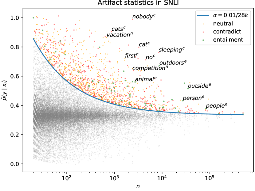
Figure 1: A statistical test for deviation from a competency problem, where no individual feature (here words) should give information about the class label, plotting the number of occurrences of each word against the conditional probability of the label given the presence of the word. The label associated with each point is marked by color and superscript. All features above the blue line have detectable correlation with class labels, using a very conservative Bonferroni-corrected statistical test.

This assumption places a very strong restriction on the problems being studied, but we argue that it is a reasonable description of complex language understanding problems. Consider, for example, the problem of sentiment analysis on movie reviews. A single feature might be the presence of the word “amazing”, which could be legitimately correlated with positive sentiment in some randomly-sampled collection of actual movie reviews. However, that correlation tells us more about word frequency in movie reviews than it tells us about a machine’s ability to understand the complexities of natural language. A competent speaker of a natural language would know that “amazing” can appear in many contexts that do not have positive sentiment and would not base their prediction on the presence of this feature alone. That is, the information about the sentiment of a review, and indeed the meaning of natural language, is contained in complex feature interactions, not in isolated features. To evaluate a machine’s understanding of language, we must remove all simple feature correlations that would allow the machine to predict the correct label without considering how those features interact.

Collecting data that accurately reflects the assumptions of a competency problem is very challenging, especially when humans are involved in creating it. Humans suffer from many different kinds of bias and priming effects, which we collectively model in this work with rejection sampling during data collection. We theoretically analyze data collection under this biased sampling process, showing that any amount of bias will result in increasing probability of statistically-significant spurious feature correlations as dataset size increases (§3).

This theoretical treatment of bias in data collection gives us a new, simple measure of data artifacts (§3.2), which we use to explore artifacts in several existing datasets (§LABEL:sec:empirical). Figure 1 revisits prior analyses on the SNLI dataset bowman-etal-2015-large with our statistical test. An analysis based on pointwise mutual information (e.g., gururangan-etal-2018-annotation) would correspond to a horizontal line in that figure, missing many features that have less extreme but still significant correlations with class labels. These less extreme correlations still lead models to overweight simple features. The problem of bias in data collection is pervasive and not easily addressed with current learning techniques.

Our framework also allows us to examine the theoretical impact of proposed techniques to mitigate bias, including performing local edits after data collection (§LABEL:sec:local-edits) and filtering collected data (§LABEL:sec:other-mitigations). We derive properties of any local edit procedure that must hold for the procedure to effectively remove data artifacts. These proofs give dataset builders tools to monitor the data collection process to be sure that resultant datasets are as artifact-free as possible. Our analysis of local edits additionally suggests a strong relationship to sensitivity in boolean functions (o2014analysis), and we identify gaps in the theory of sensitivity that need to be filled to properly account for bias in sampled datasets.

We believe our theoretical analysis of these problems provides a good starting point for future analyses of methods to improve NLP data collection, as well as insights for inductive biases that could be introduced to better model competency problems.

2 Competency Problems

We define a competency problem to be one where the marginal distribution over labels given any single feature is uniform. For our analysis, we restrict ourselves to boolean functions: we assume an input vector $\mathbf{x}$ and an output value $y$, where $\mathbf{x}\in\{0,1\}^{d}$ and $y\in\{0,1\}$. In this setting, competency means $p(y|x_{i})=0.5$ for all $i$. In other words, the information mapping $\mathbf{x}$ to $y$ is found in complex feature interactions, not in individual features.

Our core claim is that language understanding requires composing together many pieces of meaning, each of which on its own is largely uninformative about the meaning of the whole. We do not believe this claim is controversial or new, but its implications for posing language understanding as a machine learning problem are underappreciated and somewhat counterintuitive. If a model picks up on individual feature correlations in a dataset, it has learned something extra-linguistic, such as information about human biases, not about how words come together to form meaning, which is the heart of natural language understanding. To push machines towards linguistic competence, we must control for all sources of extra-linguistic information, ensuring that no simple features contain information about class labels.

For some language understanding problems, such as natural language inference, this intuition is already widely held. We find it surprising and problematic when the presence of the word “cat”, “sleeping” or even “not” in either the premise or the hypothesis gives a strong signal about an entailment decision (gururangan-etal-2018-annotation; poliak-etal-2018-hypothesis). Competency problems are broader than this, however. Consider the case of sentiment analysis. It is true that a movie review containing the word “amazing” is more likely than not to express positive sentiment about the movie. This is because of distributional effects in how humans choose to use phrases in movie reviews. These distributional effects cause the lexical semantics of “amazing” to carry over into the whole context, essentially conflating lexical and contextual cues. If our goal is to build a system that can accurately classify the sentiment of movie reviews, exploiting this conflation is useful. But if our goal is instead to build a machine that understands how sentiment is expressed in language, this feature is a red herring that must be controlled for to truly test linguistic competence.

3 Biased Sampling

To get machines to perform well on competency problems, we need data that accurately reflects the competency assumption, both to evaluate systems and (presumably) to train them. However, humans suffer from blind spots, social bias, priming, and other psychological effects that make collecting data for competency problems challenging. Examples of these effects include instructions in a crowdsourcing task that prime workers to use particular language, or distributional effects in source material, such as the “amazing” examples above, or racial bias in face recognition (Buolamwini2018GenderSI) and abusive language detection datasets (davidson-etal-2019-racial; sap2019risk).

In order to formally analyze the impact of human bias on collecting data for competency problems, we need a plausible model of this bias. We represent bias as rejection sampling from the target competency distribution based on single feature values. Specifically, we assume the following dataset collection procedure. First, a person samples an instance from an unbiased distribution $p_{u}(\mathbf{x},y)$ where the competency assumption holds. The person examines this instance, and if feature $x_{i}=1$ appears with label $y=0$, the person rejects the instance and samples a new one, with probability $r_{i}$. If $y=0$ corresponds to negative sentiment and $x_{i}$ indicates the presence of the word “amazing”, a high value for $r_{i}$ would lead to “amazing” appearing more often with positive sentiment, as is observed in typical sentiment analysis datasets.

We do not that claim rejection sampling is a plausible psychological model of dataset construction. However, we do think it is a reasonable first-order approximation of the outcome of human bias on data creation, for a broad class of biases that have empirically been found in existing datasets, and it is relatively easy to analyze.

3.1 Emergence of Artifacts Under Rejection Sampling

Let $p_{u}(y|x_{i})$ be the conditional probability of $y=1$ given $x_{i}=1$ under the unbiased distribution, $p_{b}(y|x_{i})$ be the same probability under the biased distribution, and $\hat{p}(y|x_{i})$ denote the empirical probability within a biased dataset of $n$ samples. Additionally, let $f_{i}$ be the marginal probability $p_{u}(x_{i})$. Recall that $p_{u}(y|x_{i})$ is $0.5$ by assumption.

We will say that dimension $i$ has an artifact if the empirical probability $\hat{p}(y|x_{i})$ statistically differs from $0.5$. In this section, we will show that an artifact emerges if there is a bias at dimension $i$ in the sampling procedure, which is inevitable for some features in practice. We will formalize this bias in terms of a rejection sampling probability $r_{i}$.

For a single sample $\mathbf{x},y$, we first derive the joint and marginal probabilities $p_{b}(y,x_{i})$ and $p_{b}(x_{i})$, from which we can obtain $p_{b}(y|x_{i})$. These formulas use a recurrence relation obtained from the rejection sampling procedure.

$$p_{b}(y,x_{i}) =\frac{1}{2}f_{i}+\frac{1}{2}f_{i}r_{i}p_{b}(y,x_{i})$$

$$\therefore p_{b}(y,x_{i}) =\frac{f_{i}}{2-f_{i}r_{i}}$$

$$p_{b}(x_{i}) =\frac{1}{2}f_{i}+\frac{1}{2}f_{i}(1-r_{i})+\frac{1}{2}f_{i}r_{i}p_{b}(x_{i})$$

$$\therefore p_{b}(x_{i}) =\frac{2f_{i}-f_{i}r_{i}}{2-f_{i}r_{i}}$$

$$\therefore p_{b}(y\mid x_{i}) =\frac{p_{b}(y,x_{i})}{p_{b}(x_{i})}=\frac{1}{2-r_{i}}$$

With no bias ($r_{i}=0$), this probability is $0.5$, as expected, and it rises to $1$ as $r_{i}$ increases to $1$.

We define $\hat{p}(y|x_{i})$ as the empirical expectation of $p_{b}(y|x_{i})$ over $n$ samples containing $x_{i}$, with different samples indexed by superscript $j$. $\hat{p}(y|x_{i})=\frac{1}{n}\sum_{j=1}^{n}y^{j}$. Note that $\hat{p}$ is a conditional binomial random variable. By the central limit theorem, $\hat{p}$ is approximately $\sim\mathcal{N}(\mu_{\hat{p}},\sigma_{\hat{p}}^{2})$ for large $n$, where

$$\mu_{\hat{p}} =p_{b}(y\mid x_{i})=\frac{1}{2-r_{i}}$$

$$\sigma_{\hat{p}}^{2} =\left(\frac{1-r_{i}}{(2-r_{i})^{2}}\right)^{2}\cdot\frac{1}{n}.$$

This variance is inversely proportional to the number of samples $n$. Thus, $\hat{p}(y|x_{i})$ can be well approximated by its expected value for a large number of samples. As the rejection probability $r_{i}$ increases, the center of this distribution tends from $0.5$ to $1$. This formalizes the idea that bias in the sampling procedure will cause the empirical probability $\hat{p}(y|x_{i})$ to deviate from $0.5$, even if the “true” probability is $0.5$ by assumption. Increasing the sample size $n$ concentrates the distribution inversely proportional to $\sqrt{n}$, but the expected value is unchanged. Thus, artifacts created by rejection sampling will not be combated by simply sampling more data from the same biased procedure—the empirical probability will still be biased by $r_{i}$ even if $n$ increases arbitrarily. These persistent artifacts can be exploited at i.i.d. test time to achieve high performance, but will necessarily fail if the learner is evaluated under the competency setting.

3.2 Hypothesis Test

Here we set up a hypothesis test to evaluate if there is enough evidence to reject the hypothesis that $r_{i}$ is 0, i.e., that the data is unbiased. In this case, we can use a one-sided binomial proportion hypothesis test, as our rejection sampling can only lead to binomial proportions for $p_{b}(y\mid x_{i})$ that are greater than $\frac{1}{2}$. Our null hypothesis is that the binomial proportion $p_{b}(y\mid x_{i})=0.5=p_{0}$, or equivalently, that $r_{i}=0$. Our alternative hypothesis is that $p_{b}(y\mid x_{i})\geq 0.5$. Let $\hat{p}$ be the observed probability. We can compute a $z$-statistic