Spatial Correlation Aware Compressed Sensing for User Activity Detection and Channel Estimation in Massive MTC

Abstract

Grant-free access is considered as a key enabler for massive machine-type communications (mMTC) as it promotes energy-efficiency and small signalling overhead. Due to the sporadic user activity in mMTC, joint user identification and channel estimation (JUICE) is a main challenge. This paper addresses the JUICE in single-cell mMTC with single-antenna users and a multi-antenna base station (BS) under spatially correlated fading channels. In particular, by leveraging the sporadic user activity, we solve the JUICE in a multi measurement vector compressed sensing (CS) framework under two different cases, with and without the knowledge of prior channel distribution information (CDI) at the BS. First, for the case without prior information, we formulate the JUICE as an iterative reweighted $\ell_{2,1}$-norm minimization problem. Second, when the CDI is known to the BS, we exploit the available information and formulate the JUICE from a Bayesian estimation perspective as a maximum a posteriori probability (MAP) estimation problem. For both JUICE formulations, we derive efficient iterative solutions based on the alternating direction method of multipliers (ADMM). The numerical experiments show that the proposed solutions achieve higher channel estimation quality and activity detection accuracy with shorter pilot sequences compared to existing algorithms.

I Introduction

Massive machine-type communications (mMTC) aim to provide wireless connectivity to billions of low-cost energy-constrained internet of things (IoT) devices [1]. mMTC promote three main features. First, sporadic transmissions, i.e., only an unknown subset of the IoT devices are active at a given transmission instant. Second, short-packet communications dominated by the uplink traffic. Third, energy-efficient communication protocols to ensure a long lifespan for the IoT devices, here referred to as user equipments (UEs). As the base station (BS) aims to serve a massive number of energy-constrained devices, channel access management is considered as one of the main challenges in mMTC [2]. The conventional channel access protocols, where each UE is assigned a dedicated transmission resource block, are inefficient because many resource blocks are frequently wasted as being pre-assigned to inactive UEs. Subsequently, alternative schemes have been proposed to provide more efficient channel access protocols. In particular, grant-free multiple-access has been identified as a key enabler for mMTC [3].

In the conventional grant-based channel access protocols, the active UEs first request an access to the channel, and then, the BS allocates a dedicated transmission block to each active UE in a multi-step handover process [2]. Differently, in grant-free access, the UEs transmit data as per their needs without going through the grant-based access protocols. The main advantage of grant-free access compared to conventional random access is the reduced signalling overhead and the improved energy-efficiency of the UEs. However, a paramount challenge in grant-free access is to identify the set of active UEs and to estimate their channel state information for coherent data detection. We refer to this problem as joint user identification and channel estimation (JUICE).

The sparse user activity pattern induced by the sporadic transmissions in mMTC motivates the formulation of the JUICE as a compressed sensing (CS) [4, 5, 6] problem. Furthermore, as the BS antennas sense the same sparse user activity, the JUICE problem extends to the multiple measurement vector (MMV) CS framework. Sparse support and signal recovery from an MMV setup has been studied extensively in the literature. In a nutshell, the proposed MMV sparse recovery algorithms can be categorized into the following classes: 1) greedy algorithms such as simultaneous orthogonal matching pursuit (SOMP) [7], 2) mixed norm optimization approaches [8] (and the references therein), 3) iterative methods such as approximate message passing (AMP)[9], and 4) sparse Bayesian learning (SBL) [10].

In sparse support and signal recovery algorithms, the prior knowledge on the distributions and the structure of the signals has a profound effect on the recovery performance. For instance, when the signal distribution is known, algorithms like SBL have shown superior performance compared to mixed-norm minimization [11]. However, if the signal distribution is unknown and signal statistics are not available, algorithms based on mixed-norm minimization such as $\ell_{2,1}$-norm minimization present a good choice, since they are invariant to the signal distribution. However, the $\ell_{2,1}$-norm suffers from a bias toward large coefficients in the recovery. Therefore, formulating the sparse recovery as an iterative reweighted $\ell_{1}$-norm [12] or $\ell_{2,1}$-norm [13] problem provides a significant improvement compared to their non-reweighted counterparts.

I-A Related Work

A rich line of research has been presented for grant-free access in mMTC. In [14], Chen et al. addressed the user activity detection problem in grant-free mMTC using AMP and derived an analytical performance of the proposed AMP algorithm in both single measurement vector and MMV setups. Liu et al. [15, 16] extended the analysis of [14] and conducted an asymptotic performance analysis for activity detection, channel estimation, and achievable rate. Senel and Larsson [17] designed a “non-coherent” detection scheme for very-short packet transmission by jointly detecting the active users and the transmitted information bits. Ke et al. [18] addressed the JUICE problem in an enhanced mobile broadband system and proposed a generalized AMP algorithm that exploits the channel sparsity present in both the spatial and the angular domains. Yuan et al. [19] addressed the JUICE problem in a distributed mMTC system with mixed-analog-to-digital converters under two different user traffic classes. An SBL approach has been adopted in [20] and a maximum likelihood estimation approach using the measurement covariance matrix has been considered in [21]. Recently, Ying et al. [22] presented a model-driven framework for the JUICE by utilizing CS techniques in a deep learning framework to jointly design the pilot sequences and detect the active UEs.

In addition to the sparsity of the activity pattern of the UEs, the aforementioned algorithms require different degrees of prior information on the (sparse) signal distribution. For instance, in the AMP-based approaches [14, 15, 16, 17, 21], the BS is assumed to know the distributions and the large-scale fading coefficients of channels. The work in [18] relies similarly on the known channel distributions but assumes unknown large-scale fading coefficients, which are estimated via an expectation-maximization approach.

I-B Main Contribution

This paper considers the JUICE problem in single-cell mMTC, with single-antenna UEs under spatially correlated multiple-input multiple-output (MIMO) channels. In particular, we address the JUICE under two different cases, with and without the availability of the channel distribution information (CDI) at the BS. First, under unknown CDI, the JUICE is formulated as an iterative reweighted $\ell_{2,1}$-norm minimization with a deterministic regularization penalty that accounts for the sparsity in the user activity. Second, when the CDI is available to the BS, we formulate the JUICE problem from the Bayesian perspective. By using the available knowledge on the CDI and imposing a sparsity-inducing prior on the sporadic activity of the UEs, we formulate the JUICE under a maximum a posteriori probability (MAP) estimation framework. For both JUICE formulations, we derive computationally efficient iterative solutions based on alternating direction method of multipliers (ADMM).

The vast majority of JUICE works assume that the communications channels are spatially uncorrelated and often also independent Rayleigh fading. Although this assumption may lead to analytically tractable solutions, it is not always practical as the MIMO channels are almost always spatially correlated [23]. Our paper aims to bridge this gap by addressing spatially correlated channels, which have not been widely studied in the context of JUICE in mMTC. In fact, incorporating the spatial correlation structure in the design of a JUICE solution is crucial, because the performance of JUICE solutions designed for uncorrelated channels may be sensitive to the correlation structures faced in practical scenarios [22]. Recently, Chen et al. [24] presented an orthogonal AMP algorithm to exploit both the spatial channel correlation in mMTC systems.

The main contributions of our paper can be summarized as follows:

• We address the JUICE problem in spatially correlated MIMO channels to provide a realistic assessment of the performance of the proposed JUICE solutions. Although precise knowledge of the CDI may be challenging in some practical applications, the results provide channel estimation performance benchmark for system design.

• When the BS has limited knowledge on the data structure, i.e., only the sparse behaviour of users activity is taken into consideration, we exploit the benefits of reweighting strategies in CS and formulate the JUICE as a reweighted iterative $\ell_{2,1}$-norm optimization problem. Reweighted $\ell_{2,1}$-norm minimization has not been used for JUICE problems earlier.

• When the CDI is known, we fully exploit the available information and propose a novel JUICE formulation from the Bayesian perspective. The proposed formulation relaxes non-convex Bayesian MAP estimation to convex regularization-based optimization. In particular, the CDI knowledge is incorporated via the Mahalanobis distance measure.

• For each JUICE formulation, we use a specific variable splitting strategy that allows to derive an exact ADMM solution. The proposed approach decouples the JUICE problem into a set of convex sub-problems, each admitting a computationally efficient closed-form solution that can be computed efficiently via a simple analytical formula.

• We show empirically that the proposed algorithms enhance the accuracy of user activity detection and channel estimation quality. In particular, for predefined requirements, the proposed approaches achieve the same performance as baseline MMV JUICE solutions even when using significantly smaller signalling overhead.

This paper is in line with our recent work [25, 26] where we addressed the JUICE under spatially correlated highly directive channels. In [25, 26], the JUICE was formulated as a mixed-norm minimization problem, augmented by a deterministic penalty that exploits the second-order statistics of the channels. In this paper, we further leverage the available knowledge on the entire CDI and treat the JUICE problem under a more rigorous, Bayesian framework.

Organization: The rest of the paper is organized as follows. Section II presents the system model and the canonical JUICE problem formulation. Section III addresses the JUICE with unknown CDI. Section IV derives the Bayesian formulation for the MAP-based JUICE which exploits the prior knowledge on the CDI. Simulation results are provided in Section VI, and Section VII concludes the paper.

Notations: Throughout this paper, we use boldface uppercase letters $({\bf{A}})$ to denote matrices, boldface lowercase letters $({\bf{a}})$ for vectors, and calligraphy letters $(\mathcal{S})$ to denote sets. The $i$th column of matrix ${\bf{X}}$ is denoted by ${\bf{x}}_{i}$. The transpose, the Hermitian, and the conjugate of a matrix are denoted as $(\cdot)^{\mbox{\scriptsize T}}$, $(\cdot)^{\mbox{\scriptsize H}}$, and $(\cdot)^{*}$, respectively. ${\bf{0}}$ and ${\bf{1}}$ are vectors of all entries zero and one, respectively. The $\ell_{2}$-norm and the Frobenius norm are denoted as $\|\cdot\|_{2}$ and $\|\cdot\|_{\mathrm{F}}$, respectively. $\|{\bf{a}}\|_{0}$ counts the number of non-zero entries of vector ${\bf{a}}$. $1(a)$ is an indicator function that takes the value 1 if $a\neq 0$, and 0 otherwise. $\otimes$ denotes the Kronecker product and $\mathrm{vec}(\cdot)$ denotes the operation of column-wise stacking of a matrix.

II System Model and Problem Formulation

II-A System Model

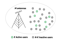
We consider a single-cell uplink mMTC system, as depicted in Fig. 1(a). The cell consists of a set $\mathcal{N}=\{1,\ldots,N\}$ uniformly distributed single-antenna UEs communicating with a BS equipped with a uniform linear array (ULA) containing $M$ antennas.

(a)

(b)

(c)

Figure 1: Illustration of a typical mMTC scenario: (a) an mMTC uplink system with $K$ active UEs and $N-K$ inactive UEs, (b) sporadic transmission, (c) division of a coherence interval $T_{\mathrm{c}}$.

We consider a block fading channel response over each coherence period $T_{\mathrm{c}}$. Furthermore, to model the propagation channels between the UEs and the BS, we consider a local scattering model, which is suitable for multi-antenna channel modelling as it can capture some key characteristics of the typical MIMO channels [27, Sect. 2.6]. In the local scattering channel model, the BS is considered to be located in an elevated position and thus, it has no scatterers in its near-field, whereas the UEs are surrounded by rich scattering environment. The channel response vector from each UE $i\in\mathcal{N}$ is modelled as the superposition of $P_{i}$ physical signal paths, each reaching the BS as a plane wave. Accordingly, the channel response vector between the $i$th UE and the BS, denoted as ${{\bf{h}}_{i}\in\mathbb{C}^{M}}$, is modelled as

$${\bf{h}}_{i}=\frac{1}{\sqrt{P_{i}}}\sum_{p=1}^{P_{i}}g_{i,p}{\bf{a}}(\psi_{i,p}),$$ (1)

where $g_{i,p}\in\mathbb{C}$ accounts for the gain and the phase-rotation of the $p$th propagation path, $\psi_{i,p}$ is the angle of arrival (AoA) of the $p$th path, and ${\bf{a}}(\psi_{i,p})\in\mathbb{C}^{M}$ is the steering vector of the ULA, defined as ${\bf{a}}(\psi_{i,p})=[1,e^{-j2\pi\Delta_{\mathrm{r}}\cos(\psi_{i,p})},\ldots,e^{-j2\pi(M-1)\Delta_{\mathrm{r}}\cos(\psi_{i,p})}]^{\mbox{\scriptsize T}}$, where $\Delta_{\mathrm{r}}$ denotes the normalized spacing between the adjacent BS antennas. We consider that $\psi_{i,p}=\bar{\psi}_{i}+\zeta_{i,p}$, where $\bar{\psi}_{i}\in[-\pi/2,\pi/2]$ represents the (deterministic) incident angle between the $i$th user and the BS, and $\zeta_{i,p}$ denotes a (random) deviation from the incident angle with angular standard deviation $\sigma_{\psi}$. We assume that each $\zeta_{i,p}$ follows a Gaussian distribution $\zeta_{i,p}\sim\mathcal{CN}(0,\,\sigma_{\psi}^{2})$ [27, Sect. 2.6].

The propagation channel between each UE and the BS is often considered to follow a complex Gaussian distribution. More specifically, by utilizing the valid assumption that the number of scatterers around each UE is very large in practice and invoking the central limit theorem, the channel vector ${\bf{h}}_{i}$ in (1) can be modelled as a complex Gaussian random variable with zero mean and covariance matrix ${\bf{R}}_{i}=\mathbb{E}[{\bf{h}}_{i}{\bf{h}}_{i}^{\mbox{\scriptsize H}}]\in\mathbb{C}^{M\times M}$ [27, Sect. 2.6], i.e.,

$${\bf{h}}_{i}\sim\mathcal{CN}(0,{\bf{R}}_{i}),\;\;P_{i}\rightarrow\infty,~{}\forall i\in\mathcal{N}.$$ (2)

The channel realizations ${\bf{h}}_{i}$ are independent between different coherence intervals $T_{\mathrm{c}}$. We consider UEs with low mobility, which is justified in the context of mMTC [28]. Hence, we adopt the common assumption that the channels are wide-sense stationary [29]. Thus, the set of channel covariance matrices $\{{\bf{R}}_{i}\}_{i=1}^{N}$ vary in a slower timescale compared to the channel realizations [30]. Accordingly, $\{{\bf{R}}_{i}\}_{i=1}^{N}$ are assumed to remain fixed for $\tau_{\mathrm{s}}$ coherence intervals, where $\tau_{\mathrm{s}}$ can be on the order of thousands [23]. We note that this assumption can be challenging in mMTC where some UEs are inactive for a longer period. Therefore, we will elaborate further on this issue in Section IV-C.

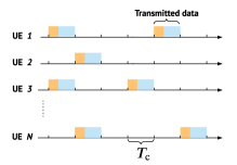
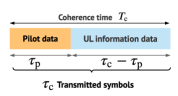
Due to the sporadic activity pattern of mMTC, only ${K<<N}$ UEs are active at each coherence interval $T_{\mathrm{c}}$, whereas the remaining $N-K$ are inactive. This is depicted in Fig. 1(b). In order to deploy a grant-free multiple access scheme, we assume that all the UEs and the BS are synchronized. In addition, each coherence interval $T_{\mathrm{c}}$ permits transmitting $\tau_{\mathrm{c}}$ symbols and is divided into two phases, as shown in Fig. 1(c). In the first phase, each active UE transmits its $\tau_{\mathrm{p}}$-length pilot sequence to the BS. In the second phase, using the remaining $\tau_{\mathrm{c}}-\tau_{\mathrm{p}}$ symbols, the active UEs send their information data to the BS. During each $T_{\mathrm{c}}$, the BS uses the transmitted pilot sequences from the first phase to identify the set of active UEs and estimate their corresponding channels in order to decode the information data transmitted at the second phase.

Regarding the channel estimation phase, the BS assigns to each UE $i\in\mathcal{N}$ a unique unit-norm pilot sequence ${\boldsymbol{\phi}}_{i}\in\mathbb{C}^{\tau_{\mathrm{p}}}$. Due to the potentially large number of UEs, the UEs cannot be assigned orthogonal pilot sequences, because it would require a pilot length of the same order as the number of UEs. Therefore, the BS assigns a set of non-orthogonal pilots which can be generated, for instance, from an independent identically distributed (i.i.d.) Gaussian or i.i.d.  Bernoulli distribution. Herein we consider pilot sequences generated from a complex symmetric Bernoulli distribution. This approach would drive the probability of pilot collision, i.e., assigning the same pilot to two distinct UEs, to be negligible [17].

Furthermore, to mitigate the channel gain differences between the UEs, a power control policy is deployed such that each UE $i\in\mathcal{N}$ transmits with a power $p^{\mathrm{UL}}_{i}$ that is inversely proportional to the average channel gain [17, 23]. Accordingly, the received signal associated with the transmitted pilots at the BS, denoted by ${\bf{Y}}\in\mathbb{C}^{\tau_{\mathrm{p}}\times M}$, is given by

$${\bf{Y}}=\sum_{i=1}^{N}\gamma_{i}\sqrt{p^{\mathrm{UL}}_{i}}{\boldsymbol{\phi}}_{i}{\bf{h}}_{i}^{\mbox{\scriptsize T}}+{\bf{W}},$$ (3)

where ${\bf{W}}\!\!\in\!\mathbb{C}^{\tau_{\mathrm{p}}\times M}$ is an additive white Gaussian noise with independent an i.i.d. elements as $\mathcal{CN}(0,\,\sigma^{2})$, and $\gamma_{i}\!\in\mathbb{B}$ is the $i$th element of the binary user activity indicator vector ${\boldsymbol{\gamma}}=[\gamma_{1},\gamma_{2},\ldots,\gamma_{N}]^{\mbox{\scriptsize T}}$, defined as

$$\gamma_{i}=\begin{cases}1,&i\in\mathcal{S}\\ 0,&\text{otherwise},\end{cases}\qquad\forall i\in\mathcal{N}$$ (4)

where $\mathcal{S}\subseteq\{1,\ldots,N\}$, ${|\mathcal{S}|=K}$, is the set of active users. We assume that besides not knowing which users are active at a given time, the BS does not either know the activity level $\frac{K}{N}$.

Let us define the effective channel of user ${i\in\mathcal{N}}$ as ${\bf{x}}_{i}=\gamma_{i}\sqrt{p^{\mathrm{UL}}_{i}}{\bf{h}}_{i}$, and subsequently, the effective channel matrix as ${\bf{X}}=[{\bf{x}}_{1},\ldots,{\bf{x}}_{N}]\in\mathbb{C}^{M\times N}$. The pilot sequence matrix is defined as ${\bf{\Phi}}=[{\boldsymbol{\phi}}_{1},\ldots,{\boldsymbol{\phi}}_{N}]\in\mathbb{C}^{\tau_{\mathrm{p}}\times N}$. Accordingly, we can rewrite the received signal associated with the pilots in (3) as

$${\bf{Y}}={\bf{\Phi}}{\bf{X}}^{\mbox{\scriptsize T}}+{\bf{W}}.$$ (5)

II-B Problem Formulation

The columns of effective channel matrix ${\bf{X}}$ corresponding to the inactive users are zeros, thus, ${\bf{X}}^{\mbox{\scriptsize T}}$ is a row-sparse matrix; it contains only $K$ non-zero rows. The objective of JUICE is to jointly identify and estimate the non-zero elements of effective channel matrix ${\bf{X}}$. Thus, JUICE can be modelled as joint support and signal recovery from an MMV setup. Subsequently, the canonical form of the JUICE can be presented as

$$\min_{{\bf{X}}}\frac{1}{2}\|{\bf{\Phi}}{\bf{X}}^{\mbox{\scriptsize T}}-{\bf{Y}}\|_{\mathrm{F}}^{2}+\beta_{1}\|{\bf{X}}^{\mbox{\scriptsize T}}\|_{2,0},$$ (6)

where $\|{\bf{X}}^{\mbox{\scriptsize T}}\|_{2,0}=\sum_{i=1}^{N}1(\|{\bf{x}}_{i}\|_{2})$ is the sparsifying regularizer and $\beta_{1}$ controls the trade-off between the emphasis on the measurement consistency term and the sparsity-promoting term. However, the $\ell_{0}$-“norm” (with slight abuse of terminology regarding a norm) minimization is an intractable combinatorial NP-hard problem. Therefore, several algorithms have been presented in the literature to relax the optimization problem (6). The existing algorithms can be categorized based on their required prior information on the signal. For instance, while AMP and SBL require prior information on the distributions of a sparse signal, mixed-norm minimization and most of the greedy algorithms operate based on the mere fact that the signal has a sparse structure.

In this paper, we cover both cases, i.e., JUICE with and without prior knowledge on the CDI. First, when there is no prior knowledge on the channel, we formulate the JUICE as an iterative reweighted $\ell_{2,1}$-norm optimization problem in Section III. Second, in Section IV, we assume that the BS has prior knowledge on the CDI, and we formulate the JUICE as a MAP estimation problem. For both these JUICE frameworks, we will derive a computationally efficient ADMM method to solve the formulated optimization problem. Each ADMM algorithm solves a relaxed version of the involved problem iteratively, and in particular, provides a closed-form solution to each sub-problem included in the optimization process.

III JUICE via Reweighted $\ell_{2,1}$-Norm Minimization

Without the CDI, the $\ell_{2,1}$-norm penalty is commonly used to relax the $\ell_{2,0}$-norm penalty in the JUICE formulation in (6) as

$$\min_{{\bf{X}}}\frac{1}{2}\|{\bf{\Phi}}{\bf{X}}^{\mbox{\scriptsize T}}-{\bf{Y}}\|_{\mathrm{F}}^{2}+\beta_{1}\|{\bf{X}}^{\mbox{\scriptsize T}}\|_{2,1}.$$ (7)

Nevertheless, unlike the democratic $\ell_{0}$-norm which penalizes the non-zero coefficients equally, $\ell_{1}$-norm is biased toward larger magnitudes, i.e., coefficients with a large magnitude are penalized more heavily than smaller ones. Therefore, striving for enhanced sparsity recovery, we use the log-sum penalty [12] to relax the $\ell_{0}$-norm in (6) as

$$\begin{array}[]{ll}&\displaystyle\min_{{\bf{X}},{\bf{u}}}\displaystyle\frac{1}{2}\|{\bf{\Phi}}{\bf{X}}^{\mbox{\scriptsize T}}-{\bf{Y}}\|_{\mathrm{F}}^{2}+\beta_{1}\sum_{i=1}^{N}\log(u_{i}+\epsilon_{0})\;\;\;\mbox{s.t.}\;\;\;\|{\bf{x}}_{i}\|_{2}\leq u_{i},~{}\forall i\in\mathcal{N},\end{array}$$ (8)

where ${\bf{u}}=[u_{1},u_{2},\ldots,u_{N}]^{\mbox{\scriptsize T}}$ is a vector of auxiliary optimization variables and $\epsilon_{0}$ is a small positive stability parameter. The log-sum penalty resembles most closely the $\ell_{2,0}$-norm penalty when $\epsilon_{0}\!\rightarrow 0$. However, a practical, numerically robust choice is to set $\epsilon_{0}$ to be slightly less than the expected norm of the non-zero rows in ${\bf{X}}^{\mbox{\scriptsize T}}$ [12].

As the objective function in (8) is a sum of a convex and a concave functions, it is not convex in general. Therefore, by applying a majorization-minimization (MM) approximation, (8) can be solved as the following iterative reweighted $\ell_{2,1}$-norm minimization problem

$${\bf{X}}^{(l+1)}=\displaystyle\min_{{\bf{X}}}\displaystyle\frac{1}{2}\big{\|}{\bf{\Phi}}{\bf{X}}^{\mbox{\scriptsize T}}-{\bf{Y}}\big{\|}_{\mathrm{F}}^{2}+\sum_{i=1}^{N}\beta_{1}g_{i}^{(l)}\|{\bf{x}}_{i}\|_{2},$$ (9)

with the weights set at iteration $(l)$ as

$$g_{i}^{(l)}=(\epsilon_{0}+\|{\bf{x}}_{i}^{(l)}\|_{2})^{-1},\forall i\in\mathcal{N}.$$ (10)

III-A IRW-ADMM Solution

The optimization problem (9) is convex and can be solved optimally using standard convex optimization techniques. However, as mMTC systems may grow large, the standard techniques can suffer from high computational complexity. As a remedy, we utilize ADMM [31] to solve (9) iteratively in a computationally efficient manner at each MM iteration $(l)$.

ADMM has been widely used to provide computationally efficient solutions to sparse signal recovery problems [32]. Apart from signal reconstruction, ADMM has also been utilized in the context of activity detection in mMTC [33, 22]. Cirik et al. [33] proposed an ADMM-based solution to multi-user support and signal detection in an SMV model, where they incorporate prior knowledge on the signal recovered from the previous transmission instants. In addition, Ying et al. [22] proposed an approximation step in ADMM similar to [32], but they solved the sub-problems through a model-driven deep learning decoder.

In contrast to the approximate solutions to problem (9) provided in [22, 32], we solve (9) exactly by adopting a variable splitting strategy different to [22, 32]. More precisely, the proposed splitting technique decomposes the objective function in (9) into two separable convex functions that can be solved efficiently via simple analytical formulas. In particular, we derive a set of update rules to solve (9) iteratively in a sequential fashion over multiple convex sub-problems, where each sub-problem admits a closed-form solution, as we will show next.

By introducing a splitting variable ${{\bf{Z}}\in\mathbb{C}^{M\times N}}$, i.e., a copy of optimization variable ${\bf{X}}$, we decompose the objective function in (9) into two separate functions: a quadratic function on the measurement fidelity over ${\bf{Z}}$ and a reweighted $\ell_{2,1}$-norm penalty over ${\bf{X}}$. Subsequently, we rewrite the optimization problem (9) as

$$\begin{array}[]{ll}({\bf{X}}^{(l+1)},{\bf{Z}}^{(l+1)})=\displaystyle\min_{{\bf{X}},{\bf{Z}}}\displaystyle\frac{1}{2}\|{\bf{\Phi}}{\bf{Z}}^{\mbox{\scriptsize T}}-{\bf{Y}}\|_{\mathrm{F}}^{2}+\sum_{i=1}^{N}\beta_{1}g_{i}^{(l)}\|{\bf{x}}_{i}\|_{2},\;\;\;\;\mbox{s.t.}\;\;{\bf{X}}={\bf{Z}}.\end{array}$$ (11)

Next, we write the augmented Lagrangian of (11) as follows

$$\begin{array}[]{ll}\mathcal{L}({\bf{X}},{\bf{Z}},{\bf{\Lambda}})=\displaystyle\frac{1}{2}\|{\bf{\Phi}}{\bf{Z}}^{\mbox{\scriptsize T}}-{\bf{Y}}\|_{\mathrm{F}}^{2}+\beta_{1}\sum_{i=1}^{N}g_{i}^{(l)}\|{\bf{x}}_{i}\|_{2}+\displaystyle\frac{\rho}{2}\|{\bf{X}}-{\bf{Z}}+\displaystyle\frac{{\bf{\Lambda}}}{\rho}\|_{\mathrm{F}}^{2}-\displaystyle\frac{\|{\bf{\Lambda}}\|_{\mathrm{F}}^{2}}{2\rho},\end{array}$$ (12)

where ${\bf{\Lambda}}=[{\boldsymbol{\lambda}}_{1},\ldots,{\boldsymbol{\lambda}}_{N}]\in\mathbb{C}^{M\times N}$ denotes the dual variable matrix containing the ADMM dual variables $\{{\boldsymbol{\lambda}}_{i}\}_{i=1}^{N}$, and $\rho$ is a positive parameter for adjusting the convergence of the ADMM.

The ADMM solves an optimization problem through sequential phases over the primal variables followed by the method of multipliers to update the dual variables [31]. Therefore, by applying the ADMM to the optimization problem (9), we first minimize (12) over the primal variable ${\bf{Z}}$ with $({\bf{X}},{\bf{\Lambda}})$ fixed, followed by minimization over the primal variable ${\bf{X}}$ with $({\bf{Z}},{\bf{\Lambda}})$ fixed. Finally, the ADMM updates the dual variable matrix ${\bf{\Lambda}}$ using the most recent updates of $({\bf{X}},{\bf{Z}})$. Thus, the ADMM for (9) consists of the following three steps:

$${\bf{Z}}^{(k+1)}:=\displaystyle\min_{{\bf{Z}}}\mathcal{L}({\bf{X}}^{(k)},{\bf{Z}},{\bf{\Lambda}}^{(k)}):=\displaystyle\min_{{\bf{Z}}}\frac{1}{2}\|{\bf{\Phi}}{\bf{Z}}^{\mbox{\scriptsize T}}-{\bf{Y}}\|_{\mathrm{F}}^{2}+\frac{\rho}{2}\|{\bf{X}}^{(k)}-{\bf{Z}}+\frac{1}{\rho}{\bf{\Lambda}}^{(k)}\|_{\mathrm{F}}^{2}$$ (13)

$${\bf{X}}^{(k+1)}\;\;:=\displaystyle\min_{{\bf{X}}}\mathcal{L}({\bf{X}},{\bf{Z}}^{(k+1)},{\bf{\Lambda}}^{(k)})\;\;\;:=\displaystyle\min_{{\bf{X}}}\sum_{i=1}^{N}\beta_{1}g_{i}^{(l)}\|{\bf{x}}_{i}\|_{2}+\frac{\rho}{2}\|{\bf{X}}-{\bf{Z}}^{(k+1)}+\frac{1}{\rho}{\bf{\Lambda}}^{(k)}\|_{\mathrm{F}}^{2}$$ (14)

$${\bf{\Lambda}}^{(k+1)}:={\bf{\Lambda}}^{(k)}+\rho\big{(}{\bf{X}}^{(k+1)}-{\bf{Z}}^{(k+1)}\big{)},$$ (15)

where the superscript $(k)$ denotes the ADMM iteration index. The derivations of the ADMM steps (13) and (14) are detailed below.

${\bf{Z}}$-update

ADMM updates the primal variable ${\bf{Z}}$ by solving the convex optimization problem (13). Thus, ${\bf{Z}}^{(k+1)}$ is obtained by setting the gradient of the objective function in (13) with respect to ${\bf{Z}}$ to zero, resulting in

$${\bf{Z}}^{(k+1)}=\big{(}\rho{\bf{X}}^{(k)}+{\bf{\Lambda}}^{(k)}+{\bf{Y}}^{\mbox{\scriptsize T}}{\bf{\Phi}}^{*}\big{)}\big{(}{\bf{\Phi}}^{\mbox{\scriptsize T}}{\bf{\Phi}}^{*}+\rho{\bf{I}}_{N}\big{)}^{-1}.$$ (16)

Note that the matrix inversion $\big{(}{\bf{\Phi}}^{*}{\bf{\Phi}}^{\mbox{\scriptsize T}}+\rho{\bf{I}}_{N}\big{)}^{-1}$ and the product ${\bf{Y}}^{\mbox{\scriptsize T}}{\bf{\Phi}}^{*}$ need to be computed only once, thus, they can be stored, reducing the overall algorithm complexity.

${\bf{X}}$-update

The optimization problem (14) can be decomposed into $N$ sub-problems as

$${\bf{x}}_{i}^{(k+1)}:=\min_{{\bf{x}}_{i}}\displaystyle\frac{\beta_{1}g_{i}^{(l)}}{\rho}\|{\bf{x}}_{i}\|_{2}+\frac{1}{2}\|{\bf{x}}_{i}-{\bf{c}}_{i}^{(k)}\|_{2}^{2},\;\;\;\forall i\in\mathcal{N},$$ (17)

where ${\bf{c}}_{i}^{(k)}={\bf{z}}_{i}^{(k+1)}-\dfrac{1}{\rho}{\boldsymbol{\lambda}}_{i}^{(k)}$ and ${\boldsymbol{\lambda}}_{i}^{(k)}$ is the $i$th column of ${\bf{\Lambda}}^{(k)}$. The problem in (17) admits a closed-form solution given by the soft thresholding operator [34] as

$${\bf{x}}_{i}^{(k+1)}=\frac{\max{\Big{\{}0,\|{\bf{c}}_{i}^{(k)}\|_{2}-\frac{\beta_{1}g_{i}^{(l)}}{\rho}\Big{\}}}}{\|{\bf{c}}_{i}^{(k)}\|_{2}}{\bf{c}}_{i}^{(k)},\quad\forall i\in\mathcal{N}.$$ (18)

Finally, the dual variable update ${\bf{\Lambda}}^{(k+1)}$ is performed using (15).

III-B Algorithm Implementation

The details for the proposed iterative reweighted ADMM (IRW-ADMM) algorithm to solve the problem (9) are summarized in Algorithm 1. As one stopping criterion, Algorithm 1 is run until the ${\bf{X}}$-update is converged, measured as $\|{\bf{X}}^{(k)}-{\bf{X}}^{(k-1)}\|_{\mathrm{F}}^{2}<\epsilon$ with a predefined tolerance parameter $\epsilon>0$, or until a maximum number of iterations $l_{\mathrm{max}}k_{\mathrm{max}}$ is reached, where $l_{\mathrm{max}}$ denotes the maximum number of iterations in the MM loop and $k_{\mathrm{max}}$ denotes the maximum number of iterations in the ADMM loop. Note that if the weight vector is fixed to ${\bf{g}}^{(l)}={\bf{1}},~{}l=1,2,\ldots$, Algorithm 1 provides the ADMM solution for optimization problem (7), which we term ADMM henceforth.

Input: 1) Pilot matrix ${\bf{\Phi}}$, 2) parameters $\beta_{1},\rho,\epsilon_{0},\epsilon,l_{\mathrm{max}},k_{\mathrm{max}}$

Output: $\hat{{\bf{X}}}$

Initialization: 1) ${\bf{X}}^{(0)},{\bf{V}}^{(0)},{\bf{Z}}^{(0)},{\boldsymbol{\Lambda}}^{(0)},k=1$, $l=1$, and 2) $\big{(}{\bf{\Phi}}^{\mbox{\scriptsize T}}{\bf{\Phi}}^{*}+\rho{\bf{I}}_{N}\big{)}^{-1}$

1 Receive ${\bf{Y}}$ at the BS, and compute and store ${\bf{Y}}^{\mbox{\scriptsize T}}{\bf{\Phi}}^{*}$

2 while $l<l_{\mathrm{max}}$  do

3       while $k<k_{\mathrm{max}}$ $\mathrm{or}$ $\|{\bf{X}}^{(k)}-{\bf{X}}^{(k-1)}\|^{2}_{\mathrm{F}}<\epsilon$ do

4             Update ${\bf{Z}}^{(k+1)}$ using (16)

5             Update ${\bf{X}}^{(k+1)}$ using (18)

6             ${\boldsymbol{\Lambda}}^{(k+1)}={\boldsymbol{\Lambda}}^{(k)}+\rho\big{(}{\bf{X}}^{(k+1)}-{\bf{Z}}^{(k+1)}\big{)}$

7             $k\leftarrow{k+1}$

8            

9      ${\bf{X}}^{(l)}\leftarrow{\bf{X}}^{(k+1)}$

10       $g_{i}^{(l)}=(\epsilon_{0}+\|{\bf{x}}_{i}^{(l)}\|_{2})^{-1},i\in\mathcal{N}$

11       $l\leftarrow{l+1}$

12      

Algorithm 1 IRW-ADMM

IV Spatial Correlation Aware JUICE via Bayesian Estimation

In this section, we propose a Bayesian formulation for JUICE when the CDI is available at the BS. We formulate the JUICE as MAP estimation and derive a computationally efficient ADMM solution for a relaxed version of the MAP problem.

IV-A MAP Estimation

The JUICE formulation presented in Section III as an iterative reweighted $\ell_{2,1}$-norm minimization (problem (9)) can be viewed as a joint support and signal recovery problem with a deterministic sparsity regularization. Such formulation presents a robust approach as it is invariant to the channel statistics, making it suitable for a broad range of channel distributions. However, the optimization problem (9) omits any available side information on the CDI. Alternatively, if the CDI is available, the JUICE problem can be formulated in a Bayesian framework to account for the fact that each unknown channel to be estimated is a realization of a random variable (vector) with the known distribution. A Bayesian sparse signal recovery framework has great potential in providing certain advantages over deterministic formulations [35].

Developing a JUICE solution from a Bayesian perspective is enabled by: 1) the fact that the propagation channels ${\bf{h}}_{i}$, $i\in\mathcal{N}$, are modeled by Gaussian distributions as shown in (2), and 2) the relatively slowly changing covariance matrices $\{{\bf{R}}_{i}\}_{i=1}^{N}$ which can be estimated with high accuracy. In the rest of the paper, we consider the common assumption that $\{{\bf{R}}_{i}\}_{i=1}^{N}$ are known to the BS [29]. The acquisition of CDI knowledge is further elaborated in Section IV-C.

Next, we utilize the prior information on the CDI and derive a Bayesian formulation for the JUICE problem. The JUICE performs two tasks in a joint fashion: 1) identification of the support of the user activity indicator vector ${\boldsymbol{\gamma}}$, and 2) estimation of the effective channel matrix ${\bf{X}}$, relying on the current estimate of ${\boldsymbol{\gamma}}$. The JUICE formulation in (9) applies a deterministic penalty that accounts for the row-sparsity of ${\bf{X}}^{\mbox{\scriptsize T}}$ which inherently captures the sparsity in ${\boldsymbol{\gamma}}$. However, in the Bayesian modelling, we treat the two variables to be estimated, ${\boldsymbol{\gamma}}$ and ${\bf{X}}$, as unknown quantities with such prior distributions that best model our knowledge on their true distributions, that is: 1) the sparse distribution of the user activity indicator vector ${\boldsymbol{\gamma}}$, and 2) the effective channel ${\bf{x}}_{i},~{}\forall i\in\mathcal{N}$, which is a random vector consisting of a multiplication of $\gamma_{i}$ and the complex Gaussian random vector ${\bf{h}}_{i}$ (i.e., ${\bf{x}}_{i}=\sqrt{p^{\mathrm{UL}}_{i}}\gamma_{i}{\bf{h}}_{i}$).

We derive joint MAP estimates $\{\hat{{\bf{X}}},\hat{{\boldsymbol{\gamma}}}\}$ by making an explicit use of the prior knowledge on the fact that the propagation channels between the UEs and the BS follow complex Gaussian distributions given in (2), under the assumption that the BS knows the estimates of the second-order statistics of the channels, i.e., the matrices $\{\hat{{\bf{R}}}_{i}\}_{i=1}^{N}$. To this end, the joint MAP estimates $\{\hat{{\bf{X}}},\hat{{\boldsymbol{\gamma}}}\}$ with respect to the posterior density given the measurement matrix ${\bf{Y}}$ is given by

$$\begin{array}[]{ll}\{\hat{{\bf{X}}},\hat{{\boldsymbol{\gamma}}}\}&=\underset{{\bf{X}},{\boldsymbol{\gamma}}}{\max}~{}\displaystyle p({\bf{X}},{\boldsymbol{\gamma}}|{\bf{Y}})\\ &=\underset{{\bf{X}},{\boldsymbol{\gamma}}}{\max}~{}\displaystyle\frac{p({\boldsymbol{\gamma}})p({\bf{X}}|{\boldsymbol{\gamma}})p({\bf{Y}}|{\bf{X}},{\boldsymbol{\gamma}})}{p({\bf{Y}})}\\ &\overset{(a)}{=}\underset{{\bf{X}},{\boldsymbol{\gamma}}}{\max}~{}\displaystyle{p({\boldsymbol{\gamma}})p({\bf{X}}|{\boldsymbol{\gamma}})p({\bf{Y}}|{\bf{X}})}\\ &\overset{}{=}\underset{{\bf{X}},{\boldsymbol{\gamma}}}{\min}~{}\displaystyle{-\log\,p({\bf{Y}}|{\bf{X}})}-\log\,p({\bf{X}}|{\boldsymbol{\gamma}})-\log\,p({\boldsymbol{\gamma}})\\ &\overset{(b)}{=}\underset{{\bf{X}},{\boldsymbol{\gamma}}}{\min}~{}\displaystyle\frac{1}{\sigma^{2}}\|{\bf{Y}}-{\bf{\Phi}}{\bf{X}}\|_{\mathrm{F}}^{2}-\log\,p({\bf{X}}|{\boldsymbol{\gamma}})-\log\,p({\boldsymbol{\gamma}})\end{array}$$ (19)

where $(a)$ follows from the Markov chain ${\boldsymbol{\gamma}}\rightarrow{\bf{X}}\rightarrow{\bf{Y}}$ and because $p({\bf{Y}})$ does not affect the maximization and $(b)$ follows from the additive Gaussian noise model in (3). The term $p({\bf{X}}|{\boldsymbol{\gamma}})$ denotes the conditional probability density function (PDF) of the effective channel ${\bf{X}}$ given the vector ${\boldsymbol{\gamma}}$, whereas the term $p({\boldsymbol{\gamma}})$ represents the prior belief on the distribution of the user activity.

Next, we elaborate in detail the choice of the prior $p({\boldsymbol{\gamma}})$ and the definition of the conditional PDF $p({\bf{X}}|{\boldsymbol{\gamma}})$. Then, having fixed these quantities, we derive an ADMM algorithm to find an approximate solution to the MAP estimation in (19).

IV-A1 Sparse prior $p({\boldsymbol{\gamma}})$

By the model assumption on the sporadic UE activity, the user activity indicator vector ${\boldsymbol{\gamma}}$ exhibits a sparse structure ($\gamma_{i}=0,\forall i\notin\mathcal{S}$). Thus, in the context of sparse recovery, we impose a sparsity prior $p({\boldsymbol{\gamma}})$ on ${\boldsymbol{\gamma}}$. For instance, given a continuous-magnitude random vector ${\boldsymbol{\theta}}\in\mathbb{C}^{N}$, a sparsity-inducing prior can be given by $p({\boldsymbol{\theta}})\propto\exp\big{(}-\textstyle\sum_{i=1}^{N}|\theta_{i}|^{p}\big{)}$, where $p\in[0,1]$ [36].

Note that setting $p=1$ results in the $\ell_{1}$-norm penalty corresponding to the Laplace density function. On the other hand, setting $p=0$ renders the optimal sparsity-inducing penalty corresponding to the $\ell_{0}$-norm. Since ${\boldsymbol{\gamma}}$ is a vector of binary elements, setting $p=0$ is equivalent to $p=1$ as it imposes the same sparsity prior $p({\boldsymbol{\gamma}})$. Subsequently, we select the prior $p({\boldsymbol{\gamma}})$ as the $\ell_{0}$-norm penalty as

$$p({\boldsymbol{\gamma}})\propto\exp\Big{(}-\sum_{i=1}^{N}1(\gamma_{i})\Big{)},$$ (20)

IV-A2 Conditional probability $p({\bf{X}}|{\boldsymbol{\gamma}})$

Since the user activity is controlled by ${\boldsymbol{\gamma}}$, the conditional probability $p({\bf{X}}|{\boldsymbol{\gamma}})$ is defined as follows. First, we note that the activity patterns of the different users are mutually independent, hence, the conditional PDF factorizes as $p({\bf{X}}|{\boldsymbol{\gamma}})=\prod_{i=1}^{N}p({\bf{x}}_{i}|\gamma_{i})$. In addition, for each user $i\in\mathcal{N}$, we distinguish the two possible cases for $p({\bf{x}}_{i}|\gamma_{i})$ as follows: 1) Conditioned on $\gamma_{i}=1$, the $i$th UE is active and ${\bf{x}}_{i}$ follows a Gaussian distribution, i.e., $p({\bf{x}}_{i}|\gamma_{i}=1)=p_{{\bf{x}}_{i}}$, where $p_{{\bf{x}}_{i}}\sim\mathcal{CN}(0,\tilde{{\bf{R}}}_{i})$ and $\tilde{{\bf{R}}}_{i}$ denotes the scaled covariance matrix defined as $\tilde{{\bf{R}}}_{i}=p^{\mathrm{UL}}_{i}\hat{{\bf{R}}}_{i}$. 2) Conditioned on $\gamma_{i}=0$, the $i$th UE is inactive, and ${\bf{x}}_{i}$ is a deterministic all-zero vector ${\bf{x}}_{i}={\bf{0}}$ with probability 1, i.e., $p({\bf{x}}_{i}|\gamma_{i}=0)=1$. Therefore, $p({\bf{X}}|{\boldsymbol{\gamma}})$ is given by

$$p({\bf{X}}|{\boldsymbol{\gamma}})=\prod_{i=1}^{N}p({\bf{x}}_{i}|\gamma_{i})=\prod_{i\in\mathcal{S}}p_{{\bf{x}}_{i}}.$$ (21)

By applying the log transformation to $p({\boldsymbol{\gamma}})$ in (20) and to $p({\bf{X}}|{\boldsymbol{\gamma}})$ in (21), and by dropping the constant terms that do not depend on ${\boldsymbol{\gamma}}$ and ${\bf{X}}$, the joint MAP estimation problem (19) can be equivalently written as

$$\{\hat{{\bf{X}}},\hat{{\boldsymbol{\gamma}}}\}=\displaystyle\min_{{\bf{X}},{\boldsymbol{\gamma}}}\frac{1}{2}\|{\bf{Y}}-{\bf{\Phi}}{\bf{X}}^{\mbox{\scriptsize T}}\|_{\mathrm{F}}^{2}+\displaystyle\beta_{1}\sum_{i=1}^{N}1(\gamma_{i})+\beta_{2}\sum_{i=1}^{N}{\bf{x}}_{i}^{\mbox{\scriptsize H}}\tilde{{\bf{R}}}_{i}^{-1}{\bf{x}}_{i},$$ (22)

where regularization weights $\beta_{1}$ and $\beta_{2}$ balance the emphasis on the priors both in relation to each other and to the measurement fidelity term. The third term in (22) applies a quadratic Mahalanobis distance measure, ${\bf{x}}_{i}^{\mbox{\scriptsize H}}\tilde{{\bf{R}}}^{-1}{\bf{x}}_{i}$, $i\in\mathcal{N}$, for active UEs in order to incorporate the knowledge of the spatial correlation matrices of the UEs into the optimization process.

IV-B MAP-ADMM Solution

The non-convex problem (22) is a mixed-integer programming problem due to involving binary optimization variables ${\boldsymbol{\gamma}}$, and is, thus, hard to solve for large $N$. In this section, we develop a computationally efficient ADMM algorithm, which is numerically illustrated to achieve great performance in Section VI.

We start by noting that the recovery of effective channel $\hat{{\bf{X}}}$ renders implicitly the vector ${\boldsymbol{\gamma}}$, i.e., finding the index set $\{i\mid\gamma_{i}\neq 0,\;i\in\mathcal{N}\}$ is equivalent to finding the index set $\{i\mid\|{\bf{x}}_{i}\|_{2}>0,\;i\in\mathcal{N}\}$. Therefore, we solve a relaxed version of the MAP estimation (22) by approximating the penalty term that depend on ${\boldsymbol{\gamma}}$ by penalty term that depend on $\|{\bf{x}}_{i}\|_{2},\;\forall i\in\mathcal{N}$.

Note that the second term $\sum_{i=1}^{N}1(\gamma_{i})$ in (22) is equivalent to an $\|{\bf{X}}\|_{2,0}$ penalty in the sense that it enforces the row-sparsity of the matrix ${\bf{X}}^{\mbox{\scriptsize T}}$. Therefore, $\sum_{i=1}^{N}1(\gamma_{i})$ can be relaxed by the log-sum penalty $\sum_{i=1}^{N}\log(\|{\bf{x}}_{i}\|_{2}+\epsilon_{0})$. Subsequently, we can eliminate ${\boldsymbol{\gamma}}$ and approximate (22) as

$$\min_{{\bf{X}},{\bf{u}}}\displaystyle\frac{1}{2}\|{\bf{Y}}-{\bf{\Phi}}{\bf{X}}^{\mbox{\scriptsize T}}\|_{\mathrm{F}}^{2}+\beta_{1}\sum_{i=1}^{N}\log(u_{i}+\epsilon_{0})+\beta_{2}\sum_{i=1}^{N}{\bf{x}}_{i}^{\mbox{\scriptsize H}}\tilde{{\bf{R}}}_{i}^{-1}{\bf{x}}_{i}\;\;\;\mbox{s.t.}\;\;\;\|{\bf{x}}_{i}\|_{2}\leq u_{i},~{}\forall i\in\mathcal{N}.$$ (23)

Again, we utilize MM and linearize the concave penalty term by its first-order Taylor expansion at point ${\bf{u}}^{(l)}$. Thus, an approximate solution to (23) is found by iteratively solving the problem

$$\begin{array}[]{ll}\hat{{\bf{X}}}^{(l+1)}=\displaystyle\min_{{\bf{X}}}\frac{1}{2}\|{\bf{Y}}-{\bf{\Phi}}{\bf{X}}^{\mbox{\scriptsize T}}\|_{\mathrm{F}}^{2}+\beta_{1}\sum_{i=1}^{N}g_{i}^{(l)}\|{\bf{x}}_{i}\|_{2}+\beta_{2}\sum_{i=1}^{N}{\bf{x}}_{i}^{\mbox{\scriptsize H}}\tilde{{\bf{R}}}_{i}^{-1}{\bf{x}}_{i},\end{array}$$ (24)

where the weight vector ${\bf{g}}^{(l)}=[g_{1}^{(l)},g_{2}^{(l)},\ldots,g_{N}^{(l)}]^{\mbox{\scriptsize T}}$ is given according to (10). The optimization problem (24) can be seen as an iterative reweighted $\ell_{2,1}$-norm minimization augmented with an additional penalty function that incorporates the spatial correlation knowledge to the optimization process by applying a Mahalanobis distance penalty on the active UEs.

The objective function in (24) is a sum of convex functions, hence, the optimization problem (24) is convex. Thus, aiming to provide a computationally efficient solution, we develop an ADMM framework that solves (24) through a set of sequential update rules, each computed in closed-form. In particular, in order to decompose (24) into a set of separate functions, we introduce two splitting variables ${\bf{Z}},{\bf{V}}\in\mathbb{C}^{M\times N}$ and rewrite the optimization problem as

$$\begin{array}[]{ll}(\hat{{\bf{X}}}^{(l+1)},\hat{{\bf{Z}}}^{(l+1)},\hat{{\bf{V}}}^{(l+1)})=&\displaystyle\min_{{\bf{X}},{\bf{Z}},{\bf{V}}}\frac{1}{2}\|{\bf{Y}}-{\bf{\Phi}}{\bf{Z}}^{\mbox{\scriptsize T}}\|_{\mathrm{F}}^{2}+\beta_{1}\sum_{i=1}^{N}g_{i}^{(l)}\|{\bf{x}}_{i}\|_{2}+\beta_{2}\sum_{i=1}^{N}{\bf{v}}_{i}^{\mbox{\scriptsize H}}\tilde{{\bf{R}}}_{i}^{-1}{\bf{v}}_{i}\\ &\mbox{s.t.}\;\;\;\quad{\bf{x}}_{i}={\bf{z}}_{i},\;\;{\bf{x}}_{i}={\bf{v}}_{i},~{}\forall i\in\mathcal{N}.\end{array}$$ (25)

The optimization problem (25) is block multi-convex, i.e., the problem is convex in one set of variables while all the other variables are fixed. Since ADMM exploits implicitly the block multi-convexity nature of (25), utilizing ADMM to solve (25) is a reasonable choice. Accordingly, the augmented Lagrangian associated with (25) is given by

$$\begin{array}[]{ll}&\mathcal{L}({\bf{X}},{\bf{Z}},{\bf{V}},{\boldsymbol{\Lambda}}_{\mathrm{z}},{\boldsymbol{\Lambda}}_{\mathrm{v}})=\displaystyle\frac{1}{2}\|{\bf{Y}}-{\bf{\Phi}}{\bf{Z}}^{\mbox{\scriptsize T}}\|_{\mathrm{F}}^{2}+\beta_{1}\displaystyle\sum_{i=1}^{N}g_{i}^{(l)}\|{\bf{x}}_{i}\|_{2}+\beta_{2}\displaystyle\sum_{i=1}^{N}{\bf{v}}_{i}^{\mbox{\scriptsize H}}\tilde{{\bf{R}}}_{i}^{-1}{\bf{v}}_{i}\\ &\displaystyle+\frac{\rho}{2}\|{\bf{X}}-{\bf{V}}+\frac{1}{\rho}{\boldsymbol{\Lambda}}_{\mathrm{v}}\|_{\mathrm{F}}^{2}+\displaystyle\frac{\rho}{2}\|{\bf{X}}-{\bf{Z}}+\displaystyle\frac{1}{\rho}{\boldsymbol{\Lambda}}_{\mathrm{z}}\|_{\mathrm{F}}^{2}-\displaystyle\frac{\|{\boldsymbol{\Lambda}}_{\mathrm{z}}\|_{\mathrm{F}}^{2}}{2\rho}-\displaystyle\frac{\|{\boldsymbol{\Lambda}}_{\mathrm{v}}\|_{\mathrm{F}}^{2}}{2\rho}.\end{array}$$ (26)

where ${\boldsymbol{\Lambda}}_{\mathrm{z}}=[{\boldsymbol{\lambda}}_{\mathrm{z}1},\ldots,{\boldsymbol{\lambda}}_{\mathrm{z}N}]\in\mathbb{C}^{M\times N}$ and ${\boldsymbol{\Lambda}}_{\mathrm{v}}=[{\boldsymbol{\lambda}}_{\mathrm{v}1},\ldots,{\boldsymbol{\lambda}}_{\mathrm{v}N}]\in\mathbb{C}^{M\times N}$ are the matrices of the ADMM dual variables.

The ADMM solution to the optimization problem (24) at the $(l)$th MM iteration is achieved by sequentially minimizing $\mathcal{L}({\bf{X}},{\bf{Z}},{\bf{V}},{\boldsymbol{\Lambda}}_{\mathrm{z}},{\boldsymbol{\Lambda}}_{\mathrm{v}})$ over the primal variables $({\bf{Z}},{\bf{V}},{\bf{X}})$, followed by dual variable $({\boldsymbol{\Lambda}}_{\mathrm{z}},{\boldsymbol{\Lambda}}_{\mathrm{v}})$ updates as follows:

$${\bf{Z}}^{(k+1)}:=\displaystyle\min_{{\bf{Z}}}\mathcal{L}({\bf{X}}^{(k)},{\bf{Z}},{\bf{V}}^{(k)},{\boldsymbol{\Lambda}}_{\mathrm{z}}^{(k)},{\boldsymbol{\Lambda}}_{\mathrm{v}}^{(k)}):=\displaystyle\min_{{\bf{Z}}}\frac{1}{2}\|{\bf{\Phi}}{\bf{Z}}^{\mbox{\scriptsize T}}-{\bf{Y}}\|_{\mathrm{F}}^{2}+\frac{\rho}{2}\|{\bf{X}}^{(k)}-{\bf{Z}}+\frac{1}{\rho}{\boldsymbol{\Lambda}}_{\mathrm{z}}^{(k)}\|_{\mathrm{F}}^{2}$$ (27)

$${\bf{V}}^{(k+1)}\!\!:=\displaystyle\min_{{\bf{V}}}\mathcal{L}({\bf{X}}^{(k)},{\bf{Z}}^{(k+1)},{\bf{V}},{\boldsymbol{\Lambda}}_{\mathrm{z}}^{(k)},{\boldsymbol{\Lambda}}_{\mathrm{v}}^{(k)})=\!\displaystyle\min_{{\bf{V}}}\beta_{2}\sum_{i=1}^{N}{\bf{v}}_{i}^{\mbox{\scriptsize H}}\tilde{{\bf{R}}}_{i}^{-1}{\bf{v}}_{i}+\frac{\rho}{2}\|{\bf{X}}^{(k)}-{\bf{V}}+\frac{{\boldsymbol{\Lambda}}_{\mathrm{v}}^{(k)}}{\rho}\|_{\mathrm{F}}^{2}$$ (28)

$$\begin{array}[]{ll}\!{\bf{X}}^{(k+1)}\!\!\!\!&:=\displaystyle\min_{{\bf{X}}}\mathcal{L}({\bf{X}},{\bf{Z}}^{(k+1)},{\bf{V}}^{(k+1)},{\boldsymbol{\Lambda}}_{\mathrm{z}}^{(k)},{\boldsymbol{\Lambda}}_{\mathrm{v}}^{(k)})\\ &:=\displaystyle\min_{{\bf{X}}}\sum_{i=1}^{N}\beta_{1}g_{i}^{(l)}\|{\bf{x}}_{i}\|_{2}+\frac{\rho}{2}\|{\bf{X}}-{\bf{Z}}^{(k+1)}+\frac{1}{\rho}{\boldsymbol{\Lambda}}_{\mathrm{z}}^{(k)}\|_{\mathrm{F}}^{2}\displaystyle+\frac{\rho}{2}\|{\bf{X}}-{\bf{V}}^{(k+1)}+\frac{1}{\rho}{\boldsymbol{\Lambda}}_{\mathrm{v}}^{(k)}\|_{\mathrm{F}}^{2}\end{array}$$ (29)

$${\boldsymbol{\Lambda}}_{\mathrm{z}}^{(k+1)}:={\boldsymbol{\Lambda}}_{\mathrm{z}}^{(k)}+\rho\big{(}{\bf{X}}^{(k+1)}-{\bf{Z}}^{(k+1)}\big{)},$$ (30)

$${\boldsymbol{\Lambda}}_{\mathrm{v}}^{(k+1)}:={\boldsymbol{\Lambda}}_{\mathrm{v}}^{(k)}+\rho\big{(}{\bf{X}}^{(k+1)}-{\bf{V}}^{(k+1)}\big{)},$$ (31)

We present the derivations of the ADMM steps (27), (28), and (29) in detail below.

${\bf{Z}}$-update

We note that the ${\bf{Z}}$-update in (27) is identical to the convex optimization problem in (13), hence, ${\bf{Z}}^{(k+1)}$ is computed using (16).

${\bf{V}}$-update

We can easily show that the ${\bf{V}}$-update in (28) can be decoupled into $N$ convex sub-problems, given by

$${\bf{v}}_{i}^{(k+1)}=\min_{{\bf{v}}_{i}}\beta_{2}{\bf{v}}_{i}^{\mbox{\scriptsize H}}\tilde{{\bf{R}}}_{i}^{-1}{\bf{v}}_{i}+\displaystyle\frac{\rho}{2}\big{\|}{\bf{x}}^{(k)}_{i}-{\bf{v}}_{i}+\displaystyle\frac{{\boldsymbol{\lambda}}_{\mathrm{v}i}^{(k)}}{\rho}\big{\|}_{2}^{2},\;\;\forall i\in\mathcal{N}.$$ (32)

The solution for (32) is obtained by setting the derivative of the objective function with respect to ${\bf{v}}_{i}$ to zero, resulting in

$$\vspace{-.2cm}{\bf{v}}_{i}^{(k+1)}=\frac{1}{\beta_{2}}\tilde{{\bf{R}}}_{i}\big{(}\frac{\rho}{\beta_{2}}\tilde{{\bf{R}}}_{i}+{\bf{I}}_{M}\big{)}^{-1}(\rho{\bf{x}}_{i}^{(k)}+{\boldsymbol{\lambda}}_{\mathrm{v}i}^{(k)}),~{}\forall i\in\mathcal{N}$$ (33)

${\bf{X}}$-update

Using the manipulations for (29) shown in Appendix A, the ${\bf{X}}$-update solves the following convex optimization problem:

$${\bf{X}}^{(k+1)}:=\min_{{\bf{X}}}\sum_{i=1}^{N}\alpha_{i}^{(k)}\|{\bf{x}}_{i}\|_{2}+\rho\|{\bf{X}}-{\bf{S}}^{(k)}\|_{\mathrm{F}}^{2},$$ (34)

where $\alpha_{i}^{(k)}=\beta_{1}g_{i}^{(l)}$ and ${\bf{S}}^{(k)}=\dfrac{1}{2}\big{(}{\bf{Z}}^{(k+1)}+{\bf{V}}^{(k+1)}-\displaystyle\frac{{\boldsymbol{\Lambda}}_{\mathrm{z}}^{(k)}+{\boldsymbol{\Lambda}}_{\mathrm{v}}^{(k)}}{\rho}\big{)}$. The problem (34) decouples into $N$ sub-problems, each admitting the closed-form solution

$${\bf{x}}_{i}^{(k+1)}=\frac{\max{\big{\{}0,\|{\bf{s}}_{i}^{(k)}\|_{2}-\frac{\alpha_{i}^{(k)}}{2\rho}\big{\}}}}{\|{\bf{s}}_{i}^{(k)}\|_{2}}{\bf{s}}_{i}^{(k)},\quad\forall i\in\mathcal{N}.$$ (35)

IV-C CDI Knowledge

MAP-ADMM operates on the assumption that the BS knows the CDI of the individual channels, i.e., $\{{\bf{R}}\}_{i=1}^{N}$. We note that the assumption that the BS knows $\{{\bf{R}}_{i}\}_{i=1}^{N}$ is widely accepted in the massive MIMO literature [27, 29]. Furthermore, a similar assumption on the availability of the CDI has been adopted in [24] that addresses JUICE in mMTC with sporadic user activity.

The acquisition of the CDI at the BS may be challenging, especially for the UEs which are inactive for a long period. Therefore, a possible solution to circumvent such an issue can be realized by deploying a training phase to estimate the CDI. The training phase can be implemented over separate channel resource blocks that are solely dedicated to estimate the CDI. In practice, the BS would consume a set of available channel resources in order to obtain an estimate of all the channel covariance matrices, denoted as $\{\hat{{\bf{R}}}_{i}\}_{i=1}^{N}$. In particular, at different time intervals, a specific group of UEs transmit pre-assigned orthogonal training pilots to the BS over $T$ coherence intervals, and subsequently, the BS employs conventional MIMO channel estimation techniques to obtain $T$ estimates of channel responses ${\bf{h}}_{i}$, denoted as $\hat{{\bf{h}}}_{i}^{1},\ldots,\hat{{\bf{h}}}_{i}^{T}$. Subsequently, the BS computes the estimated channel covariance matrix for the $i$th UE as $\hat{{\bf{R}}}_{i}=\frac{1}{T}\sum_{t=1}^{T}\hat{{\bf{h}}}_{i}^{t}\hat{{\bf{h}}}_{i}^{t^{\mbox{\scriptsize H}}}$.

The frequency of updating the CDI at the BS depends on the mobility and the activity level of the UEs as well as the changes in the multi-path environment. Therefore, the estimated $\hat{{\bf{R}}}_{i}$ can be used over several coherence intervals due to the fact that: 1) the channel covariance matrices vary in a slower timescale compared to the channel coherence time, and 2) the UEs have very low mobility in many practical mMTC systems. Consequently, learning the CDI does not consume disproportionate amount of resources. As we will show in the simulation results, the BS does not require a large number of training samples $T$ to estimate $\{{\bf{R}}\}_{i=1}^{N}$. In fact, the BS needs roughly $T=2M$ samples to provide near-optimal results in terms of the mean square error for channel estimation, and we note that similar conclusion has been reported in [27, Sect. 3.3.3].

IV-D Algorithm Implementation

The details of the proposed MAP-based JUICE, termed MAP-ADMM, are summarized in Algorithm 2. We note that ${\bf{Z}}$-update (27) and the ${\bf{V}}$-update (28) are independent from each other, hence, they can be performed fully in parallel. Similarly to Algorithm 1, MAP-ADMM is run until $\|{\bf{X}}^{(k)}-{\bf{X}}^{(k-1)}\|_{\mathrm{F}}^{2}<\epsilon$ or until a maximum number of iterations $l_{\mathrm{max}}k_{\mathrm{max}}$ is reached.

Input: 1) Pilot matrix ${\bf{\Phi}}$, covariance matrices $\{\tilde{{\bf{R}}}_{i}\}_{i=1}^{N}$, $\big{(}{\bf{\Phi}}^{\mbox{\scriptsize T}}{\bf{\Phi}}^{*}+\rho{\bf{I}}_{N}\big{)}^{-1}$, $\frac{1}{\beta_{2}}\tilde{{\bf{R}}}_{i}\big{(}\frac{\rho}{\beta_{2}}\tilde{{\bf{R}}}_{i}+{\bf{I}}_{M}\big{)}^{-1},\forall i\in\mathcal{N}$

2) parameters $\beta_{1}$,$\beta_{2}$ ,$\rho$, $\epsilon_{0}$, $\epsilon$, $\kappa$, $l_{\mathrm{max}}$,$k_{\mathrm{max}}$,

Output: $\hat{{\bf{X}}}$

Initialization: ${\bf{X}}^{(0)},{\bf{V}}^{(0)},{\bf{Z}}^{(0)},{\boldsymbol{\Lambda}}_{\mathrm{v}}^{(0)},{\boldsymbol{\Lambda}}_{\mathrm{z}}^{(0)},k=1,l=1.$

1 Receive ${\bf{Y}}$ at the BS, and compute and store while $l<l_{\mathrm{max}}$  do

2       while $k<k_{\mathrm{max}}$ $\mathrm{or}$ $\|{\bf{X}}^{(k)}-{\bf{X}}^{(k-1)}\|<\epsilon$ do

3             Update ${\bf{Z}}^{(k+1)}$ using (16) and ${\bf{V}}^{(k+1)}$ using (33)

4             Update ${\bf{X}}^{(k+1)}$ using (35)

5             ${\boldsymbol{\Lambda}}_{\mathrm{z}}^{(k+1)}={\boldsymbol{\Lambda}}_{\mathrm{z}}^{(k)}+\rho\big{(}{\bf{X}}^{(k+1)}-{\bf{Z}}^{(k+1)}\big{)}$

6             ${\boldsymbol{\Lambda}}_{\mathrm{v}}^{(k+1)}={\boldsymbol{\Lambda}}_{\mathrm{v}}^{(k)}+\rho\big{(}{\bf{X}}^{(k+1)}-{\bf{V}}^{(k+1)}\big{)}$

7             $k\leftarrow{k+1}$

8            

9      ${\bf{X}}^{(l)}\leftarrow{\bf{X}}^{(k+1)}$

10       Update $g_{i}^{(l)}$ using (10)

11       $l\leftarrow{l+1}$

12      

Algorithm 2 MAP-ADMM

V Algorithm Computational Complexity

In a typical mMTC scenario, where the number of connected devices is very large, the complexity of the recovery algorithms is an important issue to address. In fact, for the implementation of the proposed algorithms, the computational complexity determines the hardware processing cost. Next, we analyze the complexity of the proposed JUICE algorithms in terms of the number of required complex multiplications per iteration using the big $\mathcal{O}(\cdot)$ notation. The complexity analysis is summarized in Table I which also shows the exact number of matrix multiplications.

At the ${\bf{Z}}$-update step of IRW-ADMM and MAP-ADMM, for fixed $\rho$, the quantity $\big{(}{\bf{\Phi}}^{\mbox{\scriptsize T}}{\bf{\Phi}}^{*}+\rho{\bf{I}}_{N}\big{)}^{-1}$ is computed only once at an algorithm initialization. Similarly, the term ${\bf{Y}}^{\mbox{\scriptsize T}}{\bf{\Phi}}^{*}$ is computed only once upon receiving the pilot signal ${\bf{Y}}$. Therefore, computing ${\bf{Z}}^{(k+1)}$ requires $(M+1)N^{2}$ complex multiplications. For the ${\bf{V}}$-update of MAP-ADMM, the terms $\frac{1}{\beta_{2}}\tilde{{\bf{R}}}_{i}\big{(}\frac{\rho}{\beta_{2}}\tilde{{\bf{R}}}_{i}+{\bf{I}}_{M}\big{)}^{-1},\forall i\in\mathcal{N}$, in (33) need to be computed only once and can subsequently be used for several coherence intervals. Hence, MAP-ADMM requires $N(M^{2}+2M)$ complex multiplications to compute ${\bf{V}}^{(k+1)}$. The soft-threshold operators in (18) and (35) for the ${\bf{X}}$-update require $2MN$ complex multiplications. Finally, the weight vector ${\bf{g}}^{(l)}$ is computed only at the outer MM iteration level $(l)$ and it requires $MN$ complex multiplications. Therefore, the overall complexity for IRW-ADMM and MAP-ADMM is $\mathcal{O}(MN^{2})$ and $\mathcal{O}(MN^{2}+NM^{2})$, respectively.

Table I also compares the complexity of IRW-ADMM and MAP-ADMM to the three baseline algorithms that we consider in the numerical experiments: Fast alternating direction method (F-ADM) [32], simultaneous orthogonal matching pursuit (SOMP) [7], and temporal sparse Bayesian learning (T-SBL) [11]. F-ADM solves the problem (7) using an ADMM algorithm and it has computational complexity of $\mathcal{O}(M\tau_{\mathrm{p}}N)$. The greedy SOMP is reported in [18] to exhibit computational complexity of $\mathcal{O}(M\tau_{\mathrm{p}}N)$. T-SBL has computational complexity of $\mathcal{O}(N^{2}M^{3}\tau_{\mathrm{p}})$.

In summary, incorporating the channel spatial correlation information results in increased computational complexity. For instance, MAP-ADMM has higher computational complexity per iteration compared to IRW-ADMM due to incorporating the spatial structure information in the ${\bf{V}}$-update step. In addition, as the proposed IRW-ADMM and MAP-ADMM aim at providing an exact solution to the JUICE problem, they are more computationally complex than F-ADM. Nevertheless, the additional cost of the proposed algorithms is compensated for by the convergence to a more accurate solution, as we will show in the next section.

TABLE I: Computational complexity for different recovery algorithms, where $(k)$ is the iteration index and $\hat{K}$ is the estimated number of non-zero element at any particular iteration

Algorithm	Number of complex multiplications in each iteration	$\mathcal{O}(\cdot)$
IRW-ADMM	$(M+1)N^{2}+3M\hat{K}+M(N-\hat{K})+MN$	$\mathcal{O}(MN^{2})$
MAP-ADMM	$(M+1)N^{2}+NM^{2}+3M\hat{K}+M(N-\hat{K})+MN$	$\mathcal{O}(MN^{2}+NM^{2})$
F-ADM [32]	$4\tau_{\mathrm{p}}MN+5MN$	$\mathcal{O}(\tau_{\mathrm{p}}MN)$
SOMP [7]	$(2\tau_{\mathrm{p}}+1)MN+\tau_{\mathrm{p}}M^{2}+(M+1)\tau_{\mathrm{p}}(k)^{2}+(k)^{3}$	$\mathcal{O}(\tau_{\mathrm{p}}MN)$
T-SBL [11]	$2M^{3}N^{2}\tau_{\mathrm{p}}+M^{2}\tau_{\mathrm{p}}^{2}+NM^{2}\tau_{\mathrm{p}}$	$\mathcal{O}(N^{2}M^{3}\tau_{\mathrm{p}})$

VI Simulation Results

In this section, we provide simulation results to show the performance of the proposed JUICE algorithms in terms of user activity detection accuracy, channel estimation quality, and convergence rate, and compare them to existing MMV reconstruction algorithms.

VI-A Simulation Setup

We consider a single-cell of a radius of $50$ m, where the BS is surrounded by $N=200$ uniformly distributed UEs, out of which $K=10$ UEs are active at each coherence interval $T_{\mathrm{c}}$. The propagation channel between the $i$th user and the BS in (1) consists of $P_{i}=200$ paths with angular spread deviation $\sigma_{\psi}=10^{\circ}$. Each user $i=1,\ldots,N$ is assigned with a unique normalized quadratic phase shift keying (QPSK) sequence ${\boldsymbol{\phi}}_{i}$, where the QPSK pilot symbols are drawn from an i.i.d. complex Bernoulli distribution. The SNR is defined as $\text{SNR}\,\left[\text{dB}\right]=10\log_{10}\left(\frac{\mathbb{E}[\|{\bf{\Phi}}{\bf{X}}\|_{\mathrm{F}}^{2}]}{\mathbb{E}\left[\|{\bf{W}}\|_{\mathrm{F}}^{2}\right]}\right).$

VI-B Performance Metrics

The JUICE performance is quantified in terms of normalized mean square error (NMSE), support recovery rate (SRR), and the convergence rate. The NMSE is defined as $\frac{\mathbb{E}\left[\|{\bf{X}}_{\mathcal{S}}-\hat{{\bf{X}}}_{\mathcal{S}}\|_{\mathrm{F}}^{2}\right]}{\mathbb{E}\left[\|{\bf{X}}_{\mathcal{S}}\|_{\mathrm{F}}^{2}\right]}$, where ${\bf{X}}_{\mathcal{S}}$ and $\hat{{\bf{X}}}_{\mathcal{S}}$ denote the original and estimated effective channel matrix, respectively, restricted to the true active support $\mathcal{S}$. The expectation in the NMSE is computed via Monte-Carlo averaging over the randomness of effective channel matrix ${\bf{X}}$, the pilot sequence matrix ${\bf{\Phi}}$, and noise ${\bf{W}}$; thus, the NMSE is presented as the normalized average square error (NASE).

The SRR is defined as $\frac{|\mathcal{S}\cap\hat{\mathcal{S}}|}{|\mathcal{S}-\hat{\mathcal{S}}|+K}$, where $\hat{\mathcal{S}}=\{i\,\mid\;\|\hat{{\bf{x}}}_{i}\|_{2}>\epsilon_{\mathrm{thr}},\;\forall i\in\mathcal{N}\}$ denotes the detected support for a small pre-defined threshold $\epsilon_{\mathrm{thr}}$. Thus, $|\mathcal{S}\cap\hat{\mathcal{S}}|$ represents the number of correctly identified active users, whereas $|\mathcal{S}-\hat{\mathcal{S}}|$ accounts for both the number of misdetected active UEs and falsely identified inactive UEs. The SRR rate approaches 1 when $\hat{\mathcal{S}}$ is close to the true $\mathcal{S}$.

VI-C Baselines

We compare the performance of the proposed algorithms against the following algorithms that solve any MMV sparse recovery problem: 1) SOMP [7], 2) F-ADM algorithm [32], which differs from the proposed ADMM in Algorithm 1 (with ${\bf{g}}^{(l)}={\bf{1}}$) in that while ADMM provides an exact solution to (7), F-ADM solves (7) approximately by linearizing the ${\bf{X}}$-update sub-problem with the first-order Taylor expansion; 3) SPARROW, which reformulates (7) as a semi-definite programming problem [8, Eq. (22)] and we solve it using CVX toolbox [37]; and 4) T-SBL[11] where both the second-order statistics and the noise variance are known at the BS and the sparse recovery is performed using the update rules given by [11, Eqs. (6), (7), (12)] (i.e., “${\bf{B}}$-update” in [11, Eq. (13)] is not performed, because we provide the covariance matrices $\{{\bf{\hat{R}}}_{i}\}_{i=1}^{N}$.). In addition, we use both the oracle least square (LS) and the oracle joint minimum mean square error (MMSE) estimator, shown in Appendix B, where each estimator is provided “oracle” knowledge on the true set of active UEs. While the oracle LS estimator provides a good benchmark for channel estimation when no CDI is available at the BS, the joint MMSE estimator provides a lower bound on channel estimation performance when both the CDI and the noise variance is available at the BS.

VI-D Parameter Tuning

The sparse recovery algorithms require fine-tuning of their regularization parameters to yield their best estimates. While the regularization parameters depend on the different system parameters, such as $N$, $M$, $K$, $\tau_{\mathrm{p}}$, and $\sigma^{2}$, they are selected empirically by cross-validation in practice. For a fair comparison, all the parameters have been empirically tuned in advance and then fixed such that they provide overall the best performance in terms of NASE for the SNR range $[0-16]~{}$dB. For instance, $\beta_{1}$ depends highly on the ratio $\frac{K}{N}$, however, since the $K$ is not known to the BS in general, we tuned $\beta_{1}$ based on the noise variance $\sigma^{2}$ as $\beta_{1}=\sqrt{\frac{\sigma^{2}}{2}}$ since it provided the most robust convergence. Furthermore, we set $\beta_{2}$ and log-sum stability parameter $\epsilon_{0}$ to $\beta_{2}=1~{}\%$ and $\epsilon_{0}=0.07-0.12~{}\%$ of the average norm of the effective channels. Moreover, since ADMM converges typically in few tens of iterations, a maximum number of iterations of $l_{\mathrm{max}}=12$, $k_{\mathrm{max}}=5$, and stopping criterion $\epsilon=10^{-3}$ were found to be sufficient for the ADMM-based algorithms to converge to their best performance. All the optimization variables for MAP-ADMM (${\bf{X}},{\bf{V}},{\bf{Z}},{\bf{\Lambda}}_{\mathrm{z}}$, and ${\bf{\Lambda}}_{\mathrm{v}}$) and for IRW-ADMM (${\bf{X}}$, ${\bf{Z}}$, and ${\bf{\Lambda}}$) are initialized as zero matrices. The results are obtained by averaging over $10^{3}$ random channel realizations.

VI-E Results

VI-E1 Performance without Side Information

First, we examine the scenario when no CDI is available to the BS. To this end, we compare the performance of the proposed ADMM and IRW-ADMM algorithms (Algorithm 1) with F-ADM, SPARROW, SOMP, and oracle LS.

Fig. 2(a) illustrates the obtained SRR against SNR for the different sparse recovery algorithms. The obtained results reveal that the proposed IRW-ADMM provides the best performance by achieving the highest user activity detection accuracy. In fact, the IRW-ADMM using pilot sequence length $\tau_{\mathrm{p}}=20$ is able to achieve SRR $=0.95$ for ${\text{SNR}>6}$ dB. Furthermore, even with the $25~{}\%$ reduced pilot length, i.e., $\tau_{\mathrm{p}}=15$, the IRW-ADMM still outperforms the other MMV recovery algorithms by a large margin. Fig. 2(a) shows that the proposed ADMM provides similar performance F-ADM. However, we note that ADMM uses fewer regularization parameters compared to F-ADM, thus, it may be more resilient to parameter tuning.

(a) SRR versus SNR.

(b) NASE rate SNR.

Figure 2: Performance of JUICE with no side information in terms of SRR and NASE against SNR for $N=200$, $M=20$, and $K=10$.

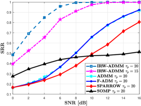
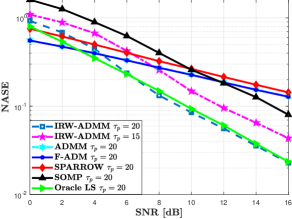
Fig. 2(b) depicts the channel estimation performance for the different recovery algorithms in terms of NASE against SNR, including the comparison to the genie-aided LS benchmark. It can be readily seen that for $\tau_{\mathrm{p}}=20$, the performance of the proposed IRW-ADMM nearly matches the performance of the genie-aided LS. Furthermore, IRW-ADMM with a reduced pilot sequence length of $\tau_{\mathrm{p}}=15$ still outperforms ADMM, F-ADM, SOMP and SPARROW for SNR $>8$ dB. Similarly to the SRR performance, the proposed ADMM and F-ADM achieve similar NASE performance. Moreover, as the sparsity regularization parameter for both F-ADM and ADMM is based on the knowledge of the noise variance, F-ADM and ADMM shows to outperform the oracle LS for SNR $<4$ dB. Finally, while SOMP provides a lower SRR performance, it outperforms ADMM, F-ADM, and SPARROW in terms of NASE for the high SNR regime. The low SRR in SOMP is caused by the high number of falsely identified inactive UEs. However, since NASE is quantified only for the true active UEs, the NASE performance does not suffer a huge degradation. In summary, the results presented in Fig. 2 highlight the remarkable gains obtained by formulating the JUICE as an iterative reweighted $\ell_{2,1}$-norm minimization problem.

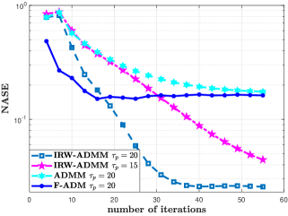
Fig. 3 presents a typical convergence behavior of ADMM, IRW-ADMM, and F-ADM for $\text{SNR}=16$ dB. The figure shows the number of iterations required for the algorithms to converge to the optimal performance. The results reveal that IRW-ADMM using $\tau_{\mathrm{p}}=20$ takes approximately $40$ iterations to convergence, with a slower convergence when reducing the pilot sequence length to $\tau_{\mathrm{p}}=15$. On the other hand, different from the SRR and NASE performance where ADMM and F-ADM provide similar performance, F-ADM converges in about 20 iterations which is much faster than the proposed ADMM taking about $50$ iterations to converge.

Figure 3: Convergence behaviour in terms of NASE versus the number of iterations at SNR $=16$ dB for $N=200$, $M=20$, and $K=10$.

VI-E2 The Impact of Exploiting Channel Statistics

Since we have shown the superiority of IRW-ADMM over conventional sparse recovery algorithms where no knowledge on the CDI is used, next, we investigate the effect of incorporating the CDI on the JUICE performance.

First, we quantify the activity detection accuracy performance of the proposed MAP-ADMM and compare it to IRW-ADMM and T-SBL. Fig. 4(a) presents the SRR against SNR for the proposed algorithms for different values of pilots lengths. The results clearly show that MAP-ADMM provides superior performance compared to IRW-ADMM. For instance, MAP-ADMM identifies the set of true active users $\mathcal{S}$ perfectly for SNR $>8$ dB using a pilot length $\tau_{\mathrm{p}}=20$. Furthermore, reducing the pilot length by a factor of $25~{}\%$ (i.e., $\tau_{\mathrm{p}}=15$) affects the performance of MAP-ADMM only moderately and optimal performance is achieved for SNR $>10$ dB. More interestingly, the results indicate that even with $40~{}\%$ reduction in the pilot sequence length (i.e., $\tau_{\mathrm{p}}=12$), MAP-ADMM provides $95~{}\%$ SRR rate for SNR $>10$ dB. Finally, the results show that while T-SBL suffers from an inferior performance in the low SNR regime, it provides an optimal activity detection performance when SNR $>8$ dB.

(a) SRR versus SNR.

(b) NASE rate SNR.

Figure 4: Performance of the proposed MAP-ADMM in terms of SRR and NASE against SNR for $N=200$, $M=20$, and $K=10$.

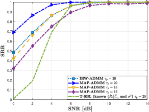
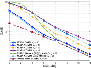
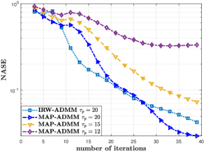
Fig. 4(b) illustrates the channel estimation performance in terms of NASE for MAP-ADMM against SNR for different pilot lengths and compares it to IRW-ADM, T-SBL, and the oracle MMSE benchmark. The proposed MAP-ADMM indisputably provides superior performance and significant improvement over IRW-ADMM. For instance, given the same pilot sequence length of $\tau_{\mathrm{p}}=20$, MAP-ADMM achieves the same performance as IRW-ADMM while using up to $6$ dB lower SNR. Furthermore, Fig. 4(b) reveals one advantageous feature of utilizing available CDI: even with 25 $\%$ reduction in the pilot length, i.e., $\tau_{\mathrm{p}}=15$, MAP-ADMM still provides 2 dB gain compared to IRW-ADMM. Comparing the performances between the MAP-ADMM and T-SBL algorithms, we distinguish two cases: 1) For ${\text{SNR}<8}$ dB, T-SBL does not provide a reliable performance and MAP-ADMM outperforms T-SBL by a large margin, or so. 2) In the high SNR regimes, i.e., $\text{SNR}\geq 8$ dB, T-SBL outperforms slightly MAP-ADMM. These results can be explained by the fact that, in contrast to MAP-ADMM, T-SBL knows and uses the exact noise variance $\sigma^{2}$. However, when the BS has the exact knowledge on the noise variance $\sigma^{2}$ as well as the CDI, the slight gap in the NASE performance between T-SBL and MAP-ADMM can be compensated for by utilizing a joint MMSE estimator on the received signal associated with the estimated active UE set $\hat{\mathcal{S}}$ obtained by MAP-ADMM. Fig. 4(b) shows that using the joint MMSE estimator on the estimated active UEs provides even the same performance as the oracle joint MMSE estimator starting from ${\text{SNR}>8}$ dB, which consolidate the results from with Fig. 4(a) where perfect recovery is attained at SNR $>8$ dB. The results shown in Fig. 4 highlight clearly the advantages of exploiting the prior information about the channel to improve the JUICE performance in terms of activity detection accuracy and channel estimation quality.

Fig. 5(a) presents a typical convergence behavior of NASE versus the number of ADMM iterations for MAP-ADMM using different pilot sequence lengths at SNR $=16$ dB. The results reveal that MAP-ADMM using $\tau_{\mathrm{p}}=20$ requires about $40$ iterations to converge, which is similar to IRW-ADMM performance. On the other hand, the results show that reducing the pilot length affects also the convergence rate of MAP-ADMM, as it takes more iterations to converge.

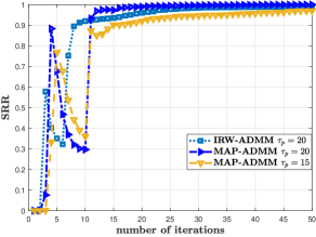
Fig. 5(b) plots the SRR performance versus the average number of ADMM iterations using different pilot lengths. MAP-ADMM using $\tau_{\mathrm{p}}=20$ achieves the perfect activity detection in 20 iterations, whereas it takes up to 40 iterations to achieve the same performance for $\tau_{\mathrm{p}}=15$. This result is interesting as MAP-ADMM needs not to run until convergence in the NASE domain, where it takes up to 40 iterations, rather, MAP-ADMM can be run for few iterations until it detects perfectly the set of active UEs (20 iterations on average) as shown in Fig. 5. Afterward, the joint MMSE estimator (39) can be applied on the estimated set of active UEs to provide the optimal channel estimation quality for the effective channel matrix, as shown in Fig. 4(b).

(a) NASE versus $(k)$.

(b) SRR rate versus $(k)$.

Figure 5: The performance of the proposed algorithms in terms of NASE and SRR versus the number of ADMM iterations for the proposed algorithms for $N=200$, $M=20$, and $K=10$.

VI-F Effect of the Number of BS Antennas

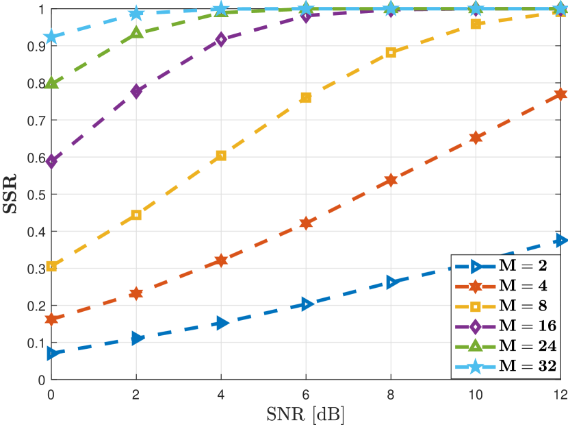
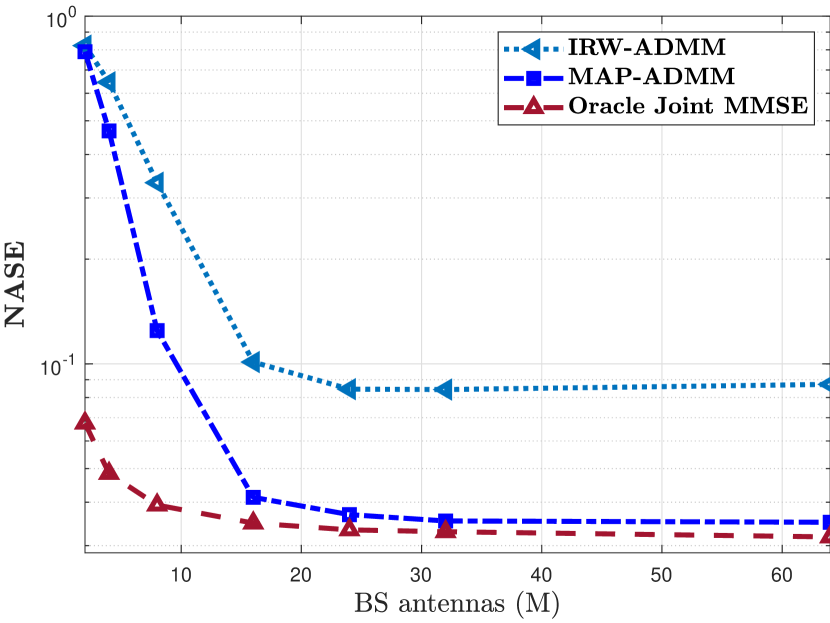
Next, we focus on quantifying the effect of the number of the BS antennas on the JUICE performance. Fig. 6(a) illustrates the SRR of MAP-ADMM versus the number of BS antennas $M$. It is clear that increasing the number of BS antennas improves significantly the active user detection accuracy. Moreover, for the low SNR regime, i.e., SNR $<8~{}$ dB, the results show the significance of increasing the number of antennas to be greater than the number of active UEs, i.e., $M>K$. However, the SRR performance starts to saturate gradually with increasing the number of BS antennas $M$. In fact, increasing the number of BS antennas from $M=8$ to $M=16$ provides more gains than increasing from $M=24$ to $M=32$; this means that the gain in SRR gradually decreases as $M$ increases. Fig. 6 (b) depicts the channel estimation performance as a function of the number of BS antennas $M$ at SNR $=12~{}$ dB. First, as expected, increasing $M$ improves NASE for all the algorithms. Moreover, by increasing $M$, the channel estimation quality obtained by MAP-ADMM improves significantly and it approaches the lower bound offered by the oracle joint MMSE. More interestingly, in contrast to activity detection accuracy where the performance saturates when $M>2K$, channel estimation quality improves considerably with the increase of $M$. Fig. 6 points out the effects of operating in massive MIMO regime, i.e., $M\!>\!K$: while user activity detection accuracy saturates around $M\!>\!2K$, channel estimation quality consistently improves when moving to the large numbers of BS antennas $M$.

(a) Activity detection.

(b) Channel estimation.

Figure 6: JUICE performance in terms of SRR and NASE versus the number of BS antennas $M$ for $N=200$, $K=10$, $\tau_{\mathrm{p}}=20$, and ${\text{SNR}=16}$ dB.

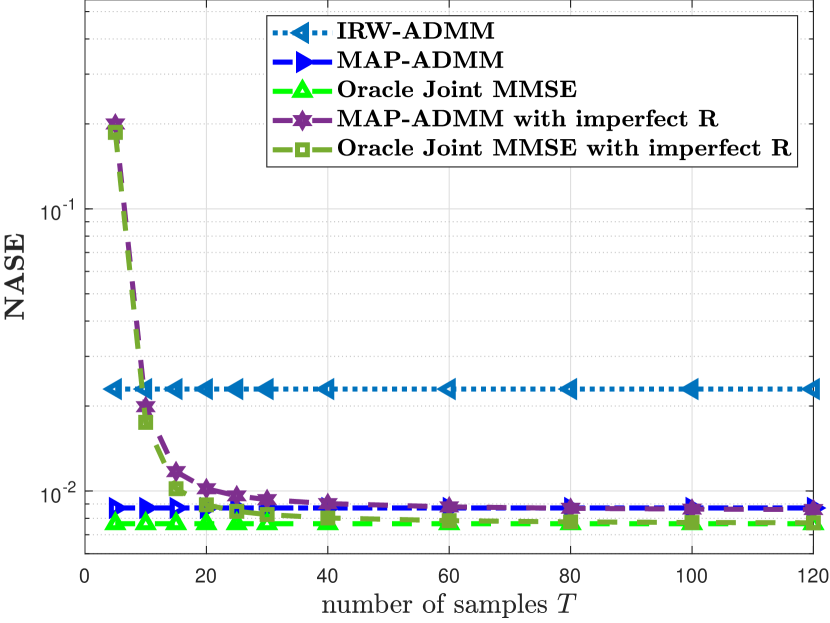
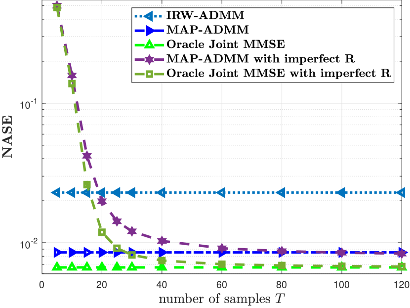
VI-G Impact of Imperfect Knowledge of the Channel Covariance Matrix

This section investigates the impact of the training phase to estimate the second-order statistics of the channels $\{\hat{{\bf{R}}}_{i}\}_{i=1}^{N}$ on the channel estimation. More precisely, we vary the number of training samples $T$ and we quantify the NASE performance of MAP-ADMM and the oracle joint MMSE estimator. Note that once the set of covariance matrices is generated using a particular number of samples $T$, it is used directly as an input to MAP-ADMM, hence, the BS does not need to update them at each MAP-ADMM iteration.

Fig. 7 depicts the NASE versus the number of samples $T$ used to generate $\{\hat{{\bf{R}}}_{i}\}_{i=1}^{N}$ for $M=20$ and $M=40$ at ${\text{SNR}=16}$ dB. The regularization parameters for MAP-ADMM and IRW-ADMM are fixed to the ones providing the best results when perfect knowledge of $\{\hat{{\bf{R}}}_{i}\}_{i=1}^{N}$ is available. First, Fig. 7 indicates that using a low number of training samples $T$ is detrimental to the performance of MAP-ADMM and the joint MMSE estimator as they require at least $T>\dfrac{M}{2}$ training samples to achieve the same performance as IRW-ADMM. Second, as expected, increasing the number of samples $T$ improves the channel estimation quality for both MAP-ADMM and the joint MMSE estimator as their NASE asymptotically approaches the lower bounds achieved by their counterparts that rely on perfect knowledge of $\{\hat{{\bf{R}}}_{i}\}_{i=1}^{N}$. More interestingly, the results show that MAP-ADMM and joint MMSE requires around $T=2M$ samples in order to a achieve the same NASE performance to their optimal lower bound. This results indicate that MAP-ADMM is not highly sensitive to imperfect channel statistics. Finally, we note that a similar conclusion on the required number samples $T$ to achieve near-optimal performance for the MMSE estimator is reported in [27, Sect. 3.3.3].

(a) $M=20$.

(b) $M=40$.

Figure 7: Channel estimation performance versus the number of samples $T$, $N=200$, $K=10$, and $\tau_{\mathrm{p}}=20$, ${\text{SNR}=16}$ dB.

VII Conclusions and Future Work

The paper addressed the JUICE problem in grant-free access in mMTC under spatially correlated fading channels. We presented two JUICE formulations depending on the availability of CDI. If no CDI is available, we proposed an iterative reweighted $\ell_{2,1}$-norm optimization problem that depends only on the sparsity of the channel matrix and it is robust and invariant to different channel distributions. When the CDI is available at the BS, we approached the JUICE from a Bayesian perspective and proposed a novel JUICE formulation based on MAP estimation. Furthermore, we derived ADMM-based algorithms that feature computationally efficient closed-form solutions that can be computed via simple analytical formulas.

The obtained numerical results highlight the following key findings. 1) Formulating the JUICE as an iterative reweighted $\ell_{2,1}$-norm minimization problem provides a huge performance improvement over conventional $\ell_{2,1}$-norm minimization. 2) While incorporating the spatial correlation of the channels increases the computational complexity of the recovery algorithms, it results in significant gains even with a smaller signalling overhead. 3) The performance of the JUICE improve dramatically when moving from the conventional MIMO regime to the massive MIMO regime. 4) The training phase for estimating the second-order statistics of the channel does not require a substantial amount of resources. Furthermore, MAP-ADMM is robust against imperfect channel statistics knowledge, which is conducive for practical use cases.

MAP-ADMM relies on the knowledge of the CDI at the BS, which may be challenging to acquire in practice. A potential future work is to design a sparse recovery algorithm that estimates the second-order statistics of the channels within the recovery process. Another interesting future direction would be to extend the JUICE framework into multi-cell and cell-free mMTC.

Appendix

VII-A Derivation of ${\bf{X}}$-update

First, recall that the ${\bf{X}}$-update (29) solves the following optimization problem:

$$\!{\bf{X}}^{(k+1)}=\displaystyle\min_{{\bf{X}}}\sum_{i=1}^{N}\alpha_{i}^{(k)}\|{\bf{x}}_{i}\|_{2}+\frac{\rho}{2}\|{\bf{X}}-\tilde{{\bf{Z}}}\|_{\mathrm{F}}^{2}+\displaystyle\frac{\rho}{2}\|{\bf{X}}-\tilde{{\bf{V}}}\|_{\mathrm{F}}^{2},$$ (36)

where $\alpha_{i}^{(k)}=\beta_{1}g_{i}^{(l)}$, $\tilde{{\bf{Z}}}={\bf{Z}}^{(k+1)}-\dfrac{{\bf{\Lambda}}_{\mathrm{z}}^{(k)}}{\rho}$, and $\tilde{{\bf{V}}}={\bf{V}}^{(k+1)}-\dfrac{{\bf{\Lambda}}_{\mathrm{v}}^{(k)}}{\rho}$. We can rewrite (36) as

$$\begin{array}[]{ll}&\!{\bf{X}}^{(k+1)}=\displaystyle\min_{{\bf{X}}}\sum_{i=1}^{N}\alpha_{i}^{(k)}\|{\bf{x}}_{i}\|_{2}+\frac{\rho}{2}\operatorname{Tr}{\bigg{(}2{\bf{X}}{\bf{X}}^{\mbox{\scriptsize H}}+\tilde{{\bf{Z}}}\tilde{{\bf{Z}}}^{\mbox{\scriptsize H}}+\tilde{{\bf{V}}}\tilde{{\bf{V}}}^{\mbox{\scriptsize H}}-{\bf{X}}^{\mbox{\scriptsize H}}\big{(}\tilde{{\bf{Z}}}+\tilde{{\bf{V}}}\big{)}-\big{(}\tilde{{\bf{Z}}}+\tilde{{\bf{V}}}\big{)}^{\mbox{\scriptsize H}}{\bf{X}}}\bigg{)}\\ &=\displaystyle\min_{{\bf{X}}}\sum_{i=1}^{N}\alpha_{i}^{(k)}\|{\bf{x}}_{i}\|_{2}+\rho\operatorname{Tr}{\bigg{(}{\bf{X}}{\bf{X}}^{\mbox{\scriptsize H}}+\frac{1}{2}\big{(}\tilde{{\bf{Z}}}\tilde{{\bf{Z}}}^{\mbox{\scriptsize H}}+\tilde{{\bf{V}}}\tilde{{\bf{V}}}^{\mbox{\scriptsize H}}\big{)}-\frac{1}{2}{\bf{X}}^{\mbox{\scriptsize H}}\big{(}\tilde{{\bf{Z}}}+\tilde{{\bf{V}}}\big{)}-\frac{1}{2}\big{(}\tilde{{\bf{Z}}}+\tilde{{\bf{V}}}\big{)}^{\mbox{\scriptsize H}}{\bf{X}}}\bigg{)},\end{array}$$ (37)

By subtracting the constant term $\dfrac{\rho}{4}\|\tilde{{\bf{V}}}-\tilde{{\bf{Z}}}\|_{\mathrm{F}}^{2}$ from (37), and denoting ${\bf{S}}^{(k)}=\dfrac{1}{2}\big{(}\tilde{{\bf{V}}}+\tilde{{\bf{Z}}}\big{)}$, the ${\bf{X}}$-update becomes (34).

VII-B Joint MMSE Estimator

The received signal in (3) can be rewritten as

$${\bf{y}}={\bf{\Theta}}_{\mathcal{S}}{\bf{x}}_{\mathcal{S}}+{\bf{w}},$$ (38)

where ${\bf{y}}\!=\!\mathrm{vec}({\bf{Y}}^{\mbox{\scriptsize T}})\!\in\!\mathbb{C}^{\tau_{\mathrm{p}}M}$, $\!{\bf{w}}\!\!=\!\!\!\mathrm{vec}({\bf{W}}^{\mbox{\scriptsize T}})\!\in\!\mathbb{C}^{\tau_{\mathrm{p}}M}$, and ${\bf{\Theta}}_{\mathcal{S}}={\boldsymbol{\Phi}}_{\mathcal{S}}\otimes{\bf{I}}_{M}\!\in\!\mathbb{C}^{M\tau_{\mathrm{p}}\times KM}$. The vectorization in (38) transforms the matrix estimation into a classical vector estimation. Thus, we utilize the MMSE estimator [38] to jointly estimate the channels of the active UEs, as

$${\bf{x}}^{\mathrm{J-MMSE}}=\mathrm{vec}({\bf{X}}^{\mathrm{J-MMSE}})=\bar{{\bf{x}}}+{\bf{R}}_{\mathrm{diag}}{\bf{\Theta}}^{\mbox{\scriptsize H}}{\bf{Q}}\big{(}{\bf{y}}-{\bf{\Theta}}\bar{{\bf{x}}}\big{)},$$ (39)

where ${\bf{Q}}=({\bf{\Theta}}{\bf{R}}_{\mathrm{diag}}{\bf{\Theta}}^{\mbox{\scriptsize H}}+\sigma^{2}{\bf{I}}_{\tau_{\mathrm{p}}M})^{-1}$, $\bar{{\bf{x}}}$ denotes the mean of ${\bf{x}}$, and ${\bf{R}}_{\mathrm{diag}}$ denotes the covariance matrix of ${\bf{x}}_{\mathcal{S}}$ given as a block diagonal matrix whose main-diagonal blocks are given by the scaled covariance matrices $\tilde{{\bf{R}}}_{i}$ corresponding to the active UEs $i\in\mathcal{S}$.

References

- [1] C. Bockelmann, N. Pratas, H. Nikopour, K. Au, T. Svensson, C. Stefanovic, P. Popovski, and A. Dekorsy, “Massive machine-type communications in 5G: Physical and MAC-layer solutions,” IEEE Commun. Mag., vol. 54, no. 9, pp. 59–65, 2016.
- [2] M. B. Shahab, R. Abbas, M. Shirvanimoghaddam, and S. J. Johnson, “Grant-free non-orthogonal multiple access for IoT: A survey,” IEEE Commun. Surveys & Tutorials, 2020.
- [3] A. C. Cirik, N. M. Balasubramanya, L. Lampe, G. Vos, and S. Bennett, “Toward the standardization of grant-free operation and the associated NOMA strategies in 3GPP,” IEEE Commun. Stand. Mag., vol. 3, no. 4, pp. 60–66, 2019.
- [4] E. J. Candés, J. Romberg, and T. Tao, “Robust uncertainty principles: Exact signal reconstruction from highly incomplete frequency information,” IEEE Trans. Inform. Theory, vol. 52, no. 2, pp. 489–509, Feb. 2006.
- [5] D. L. Donoho, “Compressed sensing,” IEEE Trans. Inform. Theory, vol. 52, no. 4, pp. 1289–1306, Apr. 2006.
- [6] J. Haupt and R. Nowak, “Signal reconstruction from noisy random projections,” IEEE Trans. Inform. Theory, vol. 52, no. 9, pp. 4036–4048, Sep. 2006.
- [7] J. A. Tropp, A. C. Gilbert, and M. J. Strauss, “Algorithms for simultaneous sparse approximation. part I: Greedy pursuit,” Signal processing, vol. 86, no. 3, pp. 572–588, 2006.
- [8] C. Steffens, M. Pesavento, and M. E. Pfetsch, “A compact formulation for the mixed-norm minimization problem,” IEEE Trans. Signal Processing, vol. 66, no. 6, pp. 1483–1497, 2018.
- [9] J. Ziniel and P. Schniter, “Efficient high-dimensional inference in the multiple measurement vector problem,” IEEE Trans. Signal Processing, vol. 61, no. 2, pp. 340–354, 2012.
- [10] D. P. Wipf and B. D. Rao, “An empirical Bayesian strategy for solving the simultaneous sparse approximation problem,” IEEE Trans. Signal Processing, vol. 55, no. 7, pp. 3704–3716, 2007.
- [11] Z. Zhang and B. D. Rao, “Sparse signal recovery with temporally correlated source vectors using sparse Bayesian learning,” IEEE J. Select. Topics Signal Processing, vol. 5, no. 5, pp. 912–926, 2011.
- [12] E. J. Candes, M. B. Wakin, and S. P. Boyd, “Enhancing sparsity by reweighted minimization,” J .FOURIER Anal. Appl., vol. 14, no. 5, pp. 877–905, 2008.
- [13] D. Wipf and S. Nagarajan, “Iterative reweighted and methods for finding sparse solutions,” IEEE J. Select. Topics Signal Processing, vol. 4, no. 2, pp. 317–329, 2010.
- [14] Z. Chen, F. Sohrabi, and W. Yu, “Sparse activity detection for massive connectivity,” IEEE Trans. Signal Processing, vol. 66, no. 7, pp. 1890–1904, 2018.
- [15] L. Liu and W. Yu, “Massive connectivity with massive MIMO—part I: Device activity detection and channel estimation,” IEEE Trans. Signal Processing, vol. 66, no. 11, pp. 2933–2946, 2018.
- [16] ——, “Massive connectivity with massive MIMO—part II: Achievable rate characterization,” IEEE Trans. Signal Processing, vol. 66, no. 11, pp. 2947–2959, 2018.
- [17] K. Senel and E. G. Larsson, “Grant-free massive MTC-enabled massive MIMO: A compressive sensing approach,” IEEE Trans. Commun., vol. 66, no. 12, pp. 6164–6175, 2018.
- [18] M. Ke, Z. Gao, Y. Wu, X. Gao, and R. Schober, “Compressive sensing-based adaptive active user detection and channel estimation: Massive access meets massive MIMO,” IEEE Trans. Signal Processing, vol. 68, pp. 764–779, 2020.
- [19] J. Yuan, Q. He, M. Matthaiou, T. Q. Quek, and S. Jin, “Toward massive connectivity for IoT in mixed-ADC distributed massive MIMO,” IEEE Internet of Things J., vol. 7, no. 3, pp. 1841–1856, 2019.
- [20] X. Zhang, Y.-C. Liang, and J. Fang, “Novel Bayesian inference algorithms for multiuser detection in M2M communications,” IEEE Trans. Veh. Technol., vol. 66, no. 9, pp. 7833–7848, 2017.
- [21] Z. Chen, F. Sohrabi, Y.-F. Liu, and W. Yu, “Covariance based joint activity and data detection for massive random access with massive MIMO,” in Proc. IEEE Int. Conf. Commun., 2019, pp. 1–6.
- [22] Y. Cui, S. Li, and W. Zhang, “Jointly sparse signal recovery and support recovery via deep learning with applications in MIMO-based grant-free random access,” IEEE J. Select. Areas Commun., vol. 39, no. 3, pp. 788–803, 2021.
- [23] E. Björnson, L. Sanguinetti, and M. Debbah, “Massive MIMO with imperfect channel covariance information,” in Proc. Annual Asilomar Conf. Signals, Syst., Comp., 2016, pp. 974–978.
- [24] Y. Cheng, L. Liu, and L. Ping, “Orthogonal AMP for massive access in channels with spatial and temporal correlations,” IEEE J. Select. Areas Commun., vol. 39, no. 3, pp. 726–740, 2021.
- [25] H. Djelouat, M. Leinonen, L. Ribeiro, and M. Juntti, “Joint user identification and channel estimation via exploiting spatial channel covariance in mMTC,” IEEE Wireless Commun. Lett, vol. 10, no. 4, pp. 887–891, 2021.
- [26] H. Djelouat, M. Leinonen, and M. Juntti, “Iterative reweighted algorithms for joint user identification and channel estimation in spatially correlated massive MTC,” in Proc. IEEE Int. Conf. Acoust., Speech, Signal Processing, 2021, pp. 4805–4809.
- [27] E. Björnson, J. Hoydis, and L. Sanguinetti, “Massive MIMO networks: Spectral, energy, and hardware efficiency,” Foundations and Trends® in Signal Processing, vol. 11, no. 3-4, pp. 154–655, 2017. [Online]. Available: http://dx.doi.org/10.1561/2000000093
- [28] A. Laya, L. Alonso, and J. Alonso-Zarate, “Is the random access channel of LTE and LTE-A suitable for M2M communications? a survey of alternatives,” IEEE Commun. Surveys & Tutorials, vol. 16, no. 1, pp. 4–16, 2013.
- [29] L. You, X. Gao, X.-G. Xia, N. Ma, and Y. Peng, “Pilot reuse for massive MIMO transmission over spatially correlated Rayleigh fading channels,” IEEE Trans. Wireless Commun., vol. 14, pp. 3352 –3366, 06 2015.
- [30] L. Sanguinetti, E. Björnson, and J. Hoydis, “Towards massive MIMO 2.0: Understanding spatial correlation, interference suppression, and pilot contamination,” IEEE Trans. Commun., vol. 68, no. 1, pp. 232–257, 2020.
- [31] S. Boyd, N. Parikh, E. Chu, B. Peleato, J. Eckstein et al., “Distributed optimization and statistical learning via the alternating direction method of multipliers,” Foundations and Trends® in Machine learning, vol. 3, no. 1, pp. 1–122, 2011.
- [32] H. Lu, X. Long, and J. Lv, “A fast algorithm for recovery of jointly sparse vectors based on the alternating direction methods,” in Proceedings of the Fourteenth International Conference on Artificial Intelligence and Statistics, 2011, pp. 461–469.
- [33] A. C. Cirik, N. M. Balasubramanya, and L. Lampe, “Multi-user detection using ADMM-based compressive sensing for uplink grant-free NOMA,” IEEE Wireless Commun. Lett, vol. 7, no. 1, pp. 46–49, 2017.
- [34] T. Goldstein, C. Studer, and R. Baraniuk, “A field guide to forward-backward splitting with a FASTA implementation,” arXiv preprint arXiv:1411.3406, 2014.
- [35] S. D. Babacan, R. Molina, and A. K. Katsaggelos, “Bayesian compressive sensing using Laplace priors,” IEEE Trans. Image Processing, vol. 19, no. 1, pp. 53–63, 2009.
- [36] D. P. Wipf and B. D. Rao, “Sparse Bayesian learning for basis selection,” IEEE Trans. Signal Processing, vol. 52, no. 8, pp. 2153–2164, 2004.
- [37] M. Grant and S. Boyd, “CVX: Matlab software for disciplined convex programming, version 2.1,” http://cvxr.com/cvx, Mar. 2014.
- [38] S. M. Kay, Fundamentals of statistical signal processing. Prentice Hall PTR, 1993.