Topological dipole Floquet solitons

Abstract

We theoretically introduce a new type of topological dipole solitons propagating in a Floquet topological insulator based on a kagome array of helical waveguides. Such solitons bifurcate from two edge states belonging to different topological gaps and have bright envelopes of different symmetries: fundamental for one component, and dipole for the other. The formation of dipole solitons is enabled by unique spectral features of the kagome array which allow the simultaneous coexistence of two topological edge states from different gaps at the same boundary. Notably, these states have equal and nearly vanishing group velocities as well as the same sign of the effective dispersion coefficients. We derive envelope equations describing components of dipole solitons and demonstrate in full continuous simulations that such states indeed can survive over hundreds of helix periods without any noticeable radiation into the bulk.

PhySH Subject Headings: Solitons; Topological insulators, Floquet insulators.

Topological insulators represent a new phase of matter characterized by qualitatively different behavior of excitations in the bulk and at the edge of these topologically nontrivial materials. The phenomenology of topological insulators, originally developed in solid state physics R1 ; R2 , was extended to diverse areas of physics, where it stimulated numerous experimental realizations, e.g. in mechanics R3 ; R4 , acoustics R5 ; R6 , in atomic R7 ; R8 , optoelectronic R9 ; R10 ; R11 , and various photonic R12 ; R13 ; R14 ; R15 ; R16 ; R17 ; R18 ; R19 systems. The significant progress made in linear topological photonics is described in reviews R20 ; R21 ; R22 , while the investigation of topological effects in nonlinear systems is still in its infancy. In such systems evolution of the topological edge states may be considerably affected by nonlinearity and a whole set of novel phenomena, ranging from topologically-protected lasing to the formation of so-called topological edge solitons, becomes possible R23 ; R24 ; R25 . Nonlinearity has been shown to impact the modulational stability of topological edge states R26 ; R27 ; R28 , the direction of topological currents R29 , the appearance of topologically nontrivial phases R30 ; R31 ; R32 , and to lead to bistability R33 . Furthermore, nonlinearity can give rise to topological closed currents in the bulk of the photonic insulator R34 ; R35 and induce a topological current at its edges R36 . Nonlinear hybridization of topological and bulk states was observed in R37 , and the valley Hall effect for vortices in nonlinear system was predicted in R38 .

Nonlinearity allows the formation of edge solitons — unique states that exhibit topological protection and simultaneously feature a rich variety of shapes and interactions. Edge solitons were predicted in photonic Floquet insulators in continuous R26 ; R34 ; R39 ; R40 and discrete R41 ; R42 ; R43 ; R44 models, and in polariton microcavities R28 ; R45 ; R46 . Their counterparts in nontopological photonic graphene were observed in R47 . Floquet Bragg solitons were reported in R48 . Topological (non-Floquet) systems also allow the formation of Dirac R49 , Bragg R50 , and valley Hall R51 edge solitons. Even though such states may in principle be encountered in many physical systems, potentially including Bose-Einstein condensates in time-modulated potentials R52 ; R53 , only fundamental edge solitons with bell-shaped amplitude profiles have been reported to date. The only exception is Floquet dark-bright states introduced in R40 , where opposite signs of the dispersion in two components dictate the dark structure of one of them — nevertheless still representing a fundamental state.

Unlike regular solitons that are rigorously defined, the corresponding concept in nonlinear Floquet insulators refers generically to the observation of localized states in nonlinear topological insulators. Here, by a Floquet soliton (FS) we denote a beam localized in the $(x,y)$-plane near the interface between topologically different materials, which bears the following two properties: it belongs to a nonlinear family bifurcating from the respective linear Floquet-Bloch edge state, and in the weakly-nonlinear limit its envelope represents a conventional soliton solution of the averaged nonlinear equation with constant coefficients. Due to the broken transversal (in the $(x,y)$-plane) and longitudinal (along the $z$-direction) translational symmetries, such states are intrinsically nonstationary, undergoing small-scale oscillations that, as our numerical simulations reported below reveal, render them effectively metastable, thus they decay during evolution albeit remarkably slowly. Thus, the envelopes of FSs analyzed here for a kagome Floquet insulator are described by soliton-bearing coupled nonlinear Schrödinger (NLS) equations with constant coefficients and they remain localized during distances that dramatically exceed longitudinal lattice helical period R26 ; R35 .

The dipole FSs introduced here are comprised of contributions from different topological gaps with envelopes of different symmetries. For the existence of such solitons, the linear edge states they bifurcate from must have equal group velocities and at the same time experience equal signs of the dispersions (understood here in terms of the Floquet-Bloch spectrum). Then the system sustains FSs where both components are bright. The dipole envelope of the weaker component in such two-dimensional (2D) states is held in shape only by the nonlinear coupling to the stronger fundamental component, as in nontopological vector dipole solitons in uniform media R54 ; R55 ; R56 ; R57 . Dipole FSs are hybrid objects that are confined to the edge due to their topological nature, while the nonlinear self-phase modulation enables their localization along the edge. This is in contrast to conventional scalar 2D dipole solitons characterized by identical localization mechanism in two transverse dimensions R58 ; R59 ; R60 ; R61 .

The propagation of light along the $z$-axis of a helical kagome array with focusing cubic nonlinearity is governed by the nonlinear Schrödinger (NLS) equation for the dimensionless field amplitude $\psi$:

$$\begin{split}i\frac{\partial\psi}{\partial z}=-\frac{1}{2}{{\Delta}_{\bot}}\psi-\mathcal{R}(\mathbf{r},z)\psi-{{\left|\psi\right|}^{2}}\psi\,.\end{split}$$ (1)

Here $\mathbf{r}=\mathbf{i}x+\mathbf{j}y$ is the radius-vector in the transverse plane, $x,y$ are the normalized transverse coordinates, ${{\Delta}_{\bot}}={{\partial}^{2}}/\partial{{x}^{2}}+{{\partial}^{2}}/\partial{{y}^{2}}$; $z$ is the normalized propagation distance and the refractive index profile is described by the function $\mathcal{R}(\mathbf{r},z)=\mathcal{R}(\mathbf{r},z+T)=\mathcal{R}(\mathbf{r}+L\mathbf{j},z)$. The array is comprised of identical waveguides of width $\sigma$ placed in the nodes ${{\mathbf{r}}_{nm}}$ of the kagome grid $\mathcal{R}(\mathbf{r},z)=p\sum\nolimits_{nm}{{{e}^{-{{[\mathbf{r}-{{\mathbf{r}}_{nm}}-\mathbf{s}(z)]}^{2}}/{{\sigma}^{2}}}}}$, where $p$ is the array depth, and $\mathbf{s}(z)={{r}_{0}}(\sin(\omega z),\cos(\omega z)-1)$ describes helical trajectory of each waveguide with the Floquet period $T=2\pi/\omega$ and radius ${{r}_{0}}$ [Fig. 1(a)]. The $y$-period of such array is $L=2d$, where $d$ is the separation between waveguides. To obtain edge states, we truncate the array in the $x$-plane to form zigzag boundaries [Fig. 1(d)]. Typical parameters of such structures are $d\sim 1.9$ ($19\;\mu\text{m}$ spacing), ${{r}_{0}}\sim 0.0-1.0$ (helix radius up to $10\;\mu\text{m}$), $p\sim 12$ (refractive index $\delta n\sim 9\times{{10}^{-4}}$), $\sigma\sim 0.4$ ($4\;\mu\text{m}$ wide waveguides), $T\sim 0-10$ (helix periods up to $12\;\text{mm}$). We assume excitation at $\lambda=800\;\text{nm}$. Arrays with such parameters can be readily created by femtosecond laser inscription R17 . Notice that topological protection of linear and nonlinear scalar modes in Floquet insulators with helical channels and similar array parameters have been shown in Refs. R26 ; R40 , therefore we expect the same degree of protection also for the dipole vector states analyzed below.

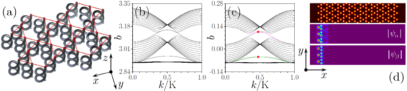
Figure 1: (a) Schematics of a kagome array of helical waveguides. (b) Dependencies $b(k)$ showing three upper bands from the Bloch spectrum for a finite array [see array profile in Fig. 1(d)] with straight waveguides $({{r}_{0}}=0)$. (c) Quasi-propagation-constants $b(k)$ defined modulo $\omega$ for a finite kagome array with helical channels at ${{r}_{0}}=0.6$, $T=8$. Red dots indicate edge states from different gaps with equal velocities $\partial{{b}_{\alpha,\beta}}/\partial k$. (d) Three periods of finite kagome array (top) and linear Floquet eigenmodes ${{\psi}_{\alpha,\beta}}$ from the left edge (middle and bottom) at $z=0$, $k=0.472\operatorname{K}$ corresponding to the red dots in (c). Here and below $p=12$, $d=1.9$, $\sigma=0.4$.

Linear eigenmodes of the helical array are Floquet-Bloch waves $\psi(\mathbf{r},z)={{\phi}_{\nu k}}(\mathbf{r},z){{e}^{i{{b}_{\nu k}}z}}$, where ${{\phi}_{\nu k}}(\mathbf{r},z)={{u}_{\nu k}}(\mathbf{r},z){{e}^{iky}}$ and the function ${{u}_{\nu k}}(\mathbf{r},z)={{u}_{\nu k}}(\mathbf{r},z+T)={{u}_{\nu k}}(\mathbf{r}+L\mathbf{j},z)$ is periodic along both $z$ and $y$ axes. Here $k$ denotes the Bloch momentum in the first Brillouin zone $k\in[-\operatorname{K}/2,+K/2)$, where $\operatorname{K}=2\pi/L$, $\nu$ is the mode index, while ${{b}_{\nu k}}\in[-\omega/2,+\omega/2)$ is a quasi-propagation-constant defined modulo $\omega$ and describing the phase ${{b}_{\nu k}}T$ accumulated by the Floquet-Bloch wave over one $z$-period. A representative spectrum of a truncated kagome array with straight waveguides (in this case, at ${{r}_{0}}=0$, $b$ is a standard propagation constant) is presented in Fig. 1(b) (for brevity, we omit subscripts in ${{b}_{\nu k}}$ in the figures). We show three upper bands, the lowest of which is nearly flat. Two pairs of degenerate edge states are clearly visible in the spectrum. For any non-zero helix radius ${{r}_{0}}\neq 0$, the system becomes topologically nontrivial as time-reversal symmetry is broken R62 ; R63 ; R64 . As a result, topological states occur on the left edge (we assign indices $\nu=\alpha,\beta$ to the “top” and “bottom” states) as marked by magenta and green lines in Fig. 1(c). Representative profiles of Floquet-Bloch waves from different gaps are shown in Fig. 1(d) (at $z=0$).

A remarkable property of the kagome topological insulator is that the derivatives ${{{b}^{\prime}}_{\nu}}=\partial{{b}_{\nu k}}/\partial k$, defining the group velocities ${{v}_{\nu}}=-{{{b}^{\prime}}_{\nu}}$ of two topological states coexisting at a given edge (see Appendix A for details) may coincide for certain values of the Bloch momentum $k$ [see, e.g. the red dots in Fig. 2(a)]. Importantly, the sign of the dispersion coefficients ${{{b}^{\prime\prime}}_{\nu}}={{\partial}^{2}}{{b}_{\nu k}}/\partial{{k}^{2}}$ for the momentum corresponding to the red dots is likewise identical [Fig. 2(b)]. Coexistence of topological edge states with coinciding group velocities ${{v}_{\alpha}}={{v}_{\beta}}$ and equal signs of the effective diffraction in the underlying linear system is necessary for the formation of multipole FSs as it allows for persistent nonlinearity- mediated coupling. For our parameters, the group velocities coincide at $k=0.472{K}$ (see Fig. 2).

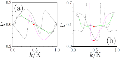
Figure 2: Derivatives ${{b}^{\prime}_{\nu}}$ (a) and ${{b}^{\prime\prime}_{\nu}}$ (b) for the edge state branches. Solid (dashed) lines correspond to the states from left (right) edges. Red dots indicate states from the left edge with equal group velocities ${{b}^{\prime\prime}_{\alpha,\beta}}=-0.00033$ and negative dispersion ${{b}^{\prime\prime}_{\alpha}}=-0.67331$, ${{b}^{\prime\prime}_{\beta}}=-0.16827$ from which FSs bifurcate (see below). The color coding for different branches is the same as in Fig. 1(c).

To construct multipole FSs we focus on their bifurcation from the linear Floquet-Bloch states ${{\psi}_{\alpha k}}$ and ${{\psi}_{\beta k}}$. To this end we look for the solution in the form $\psi\approx{{A}_{\alpha}}(Y,z){{\phi}_{\alpha k}}{{e}^{i{{b}_{{}^{\alpha k}}}z}}+{{A}_{\beta}}(Y,z){{\phi}_{\beta k}}{{e}^{i{{b}_{\beta k}}z}}$, where ${{A}_{\alpha,\beta}}$ are the slowly-varying envelopes and $Y=y-{{v}_{\alpha,\beta}}z$ is the coordinate in the frame moving with velocity ${{v}_{\alpha,\beta}}=-{{{b}^{\prime}}_{\alpha,\beta}}$, identical for both components. We adopt a multiscale expansion that shows that the envelopes ${{A}_{\alpha,\beta}}$ are governed by the coupled focusing NLS equations (see Appendix A):

$$\begin{split}i\frac{\partial{{A}_{\alpha,\beta}}}{\partial z}=&\frac{{{{{b}^{\prime\prime}}}_{\alpha,\beta}}}{2}\frac{{{\partial}^{2}}{{A}_{\alpha,\beta}}}{\partial{{Y}^{2}}}\\ &\quad-({{\chi}_{\alpha,\beta}}{{\left|{{A}_{\alpha,\beta}}\right|}^{2}}+2{{\chi}_{\operatorname{x}}}{{\left|{{A}_{\beta,\alpha}}\right|}^{2}}){{A}_{\alpha,\beta}}\,,\end{split}$$ (2)

where ${{\chi}_{\nu}}={{\langle({{\left|{{\phi}_{\nu k}}\right|}^{2}},{{\left|{{\phi}_{\nu k}}\right|}^{2}})\rangle}_{T}}$ and ${{\chi}_{\operatorname{x}}}={{\langle({{\left|{{\phi}_{\alpha k}}\right|}^{2}},{{\left|{{\phi}_{\beta k}}\right|}^{2}})\rangle}_{T}}$ are the effective self- and cross-modulation coefficients, averaging over one $z$-period is defined as ${{\langle g\rangle}_{T}}={{T}^{-1}}\int_{0}^{T}{g(\mathbf{r},z)dz}$, and calculation of the inner product $(f,g)=\int_{S}{{{f}^{*}}(\mathbf{r},z)g(\mathbf{r},z)d\mathbf{r}}$ is performed over the entire transverse array area $S$. Floquet-Bloch states ${{\phi}_{\nu k}}$ are orthogonal and normalized at the same instant $z$ (see Appendix A): $({{\phi}_{\nu k}},{{\phi}_{{\nu}^{\prime}k}})={{\delta}_{\nu{\nu}^{\prime}}}$. Note that the considerable difference between quasi- propagation-constant mismatch $\delta{{b}_{k}}={{b}_{\alpha k}}-{{b}_{\beta k}}\approx 0.15$ and frequency of periodic modulation $(\omega\approx 0.78)$ ensures that coupling between the modes is entirely non-resonant and therefore exclusively mediated by nonlinearity. Efficient nonlinear coupling between waves with different momenta $k$ can only occur for a special ratio of propagation constants of the involved topological states, which is not met in our system.

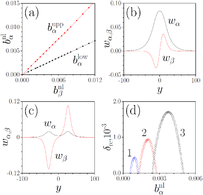
Figure 3: (a) Domain of dipole soliton existence on the $(b_{\alpha}^{\operatorname{nl}},b_{\beta}^{\operatorname{nl}})$ plane. Dipole soliton envelopes at $b_{\alpha}^{\operatorname{nl}}=0.0015$ (b) and $b_{\alpha}^{\operatorname{nl}}=0.0027$ (c) for $b_{\beta}^{\operatorname{nl}}=0.0022$. (d) Maximal real part of perturbation growth rate versus $b_{\alpha}^{\operatorname{nl}}$ at $b_{\beta}^{\operatorname{nl}}=0.001$ (curve 1), $0.0022$ (curve 2), and $0.004$ (curve 3). The parameters in the envelope equation at $k=0.472{K}$ are ${{b}^{\prime}_{\alpha}}={{b}^{\prime}_{\beta}}=-0.00033$, ${{b}^{\prime\prime}_{\alpha}}=-0.67331$, ${{b}^{\prime\prime}_{\beta}}=-0.16827$, ${{\chi}_{\alpha}}=0.31048$, ${{\chi}_{\beta}}=0.36011$, ${{\chi}_{\operatorname{x}}}=0.31973$.

We are interested in bright dipole soliton solutions of Eqs. (2) that exist at ${{b}^{\prime\prime}_{\alpha}},{{b}^{\prime\prime}_{\beta}}<0$ [see Fig. 2(b)]. In such states the bell-shaped $\alpha$ component prevents (by creating an effective potential well via cross-phase modulation) out-of-phase poles of the dipole $\beta$ component from splitting, leading to the formation of stationary states. They can be found by the Newton method in the form ${{A}_{\alpha,\beta}}={{w}_{\alpha,\beta}}{{e}^{ib_{\alpha,\beta}^{\operatorname{nl}}z}}$, where the nonlinearity-induced phase shifts $b_{\alpha,\beta}^{\operatorname{nl}}$ should be sufficiently small (much smaller than the quasi-propagation constants, the topological-gap width, and longitudinal Brillouin zone $\omega$) to ensure that the profiles ${{w}_{\alpha,\beta}}$ are broad and satisfy the assumption of slow variation of the soliton profile. The properties of dipole solitons for nonlinear and dispersion coefficients corresponding to the edge states at $k=0.472\operatorname{K}$ are described in Fig. 3. For a fixed $b_{\beta}^{\operatorname{nl}}$ dipole solitons exist for $b_{\alpha}^{\operatorname{low}}\leq b_{\alpha}^{\operatorname{nl}}\leq b_{\alpha}^{\operatorname{upp}}$. The existence domain expands with $b_{\beta}^{\operatorname{nl}}$ [Fig. 3(a)]. Close to its lower border $b_{\alpha}^{\operatorname{low}}$ the dipole $\beta$ component vanishes and only fundamental $\alpha$ component remains, while at the upper border $b_{\alpha}^{\operatorname{upp}}$ the soliton splits into two states gradually separating as the amplitude of the $\alpha$ component vanishes. Representative profiles are shown in Fig. 3(b) and 3(c). By substituting the perturbed envelope solitons ${{A}_{\nu}}=({{w}_{\nu}}+{{\mu}_{\nu}}{{e}^{\delta z}}+\eta_{\nu}^{*}{{e}^{{{\delta}^{*}}z}}){{e}^{ib_{\nu}^{\operatorname{nl}}z}}$, where ${{\mu}_{\nu}},{{\eta}_{\nu}}\ll{{w}_{\nu}}$, into Eq. (2) one arrives at a linear eigenvalue problem (see Appendix B), whose solution yields the growth rate ${{\delta}_{\operatorname{re}}}=\operatorname{Re}\delta$ for the most unstable perturbation depicted in Fig. 3(d) as a function of $b_{\alpha}^{\operatorname{nl}}$. The growth rate ${{\delta}_{\operatorname{re}}}$ vanishes when $b_{\alpha}^{\operatorname{nl}}\to b_{\alpha}^{\operatorname{low}},b_{\alpha}^{\operatorname{upp}}$ and for the broad states considered here it remains well below ${{10}^{-3}}$ implying that the characteristic scale $1/{{\delta}_{\operatorname{re}}}$ of the instability development exceeds hundreds of helix periods $T$.

To confirm the accuracy of the model (2) and to confirm that topological dipole solitons are observable experimentally, we propagated Floquet-Bloch modes with exact dipole soliton envelopes, obtained from Eq. (2) for various $b_{\alpha,\beta}^{\operatorname{nl}}$ values, in the helical kagome array. Such evolution is governed by the full 2D model (1), which we solved with a split-step FFT method. The input for Eq. (1) was constructed as $\psi={{w}_{\alpha}}(Y){{\phi}_{\alpha k}}+{{w}_{\beta}}(Y){{\phi}_{\beta k}}$. In the right column of Fig. 4(a)-(c) we show (with dots) the modulus of the projections of the field $\psi$ on the linear Floquet-Bloch modes: ${{c}_{\nu}}=\int_{mL-d}^{mL+d}{\phi_{\nu k}^{*}(\mathbf{r},z)\psi(\mathbf{r},z)d\mathbf{r}}$ ($m\in\mathbb{Z}$ defines the $y$-period on which projection is calculated), and the input envelopes ${{w}_{\alpha,\beta}}$ (solid lines). The projections ${{c}_{\nu}}$ explicitly show that dipole soliton at all distances shown contains contributions from two Floquet-Bloch states, whose amplitudes remain practically unchanged and whose envelopes remain mutually localized.

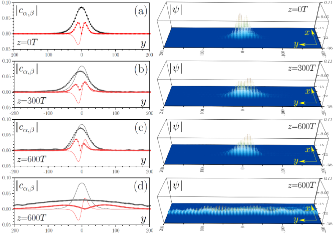
Figure 4: Propagation of a dipole topological quasi-soliton in Eq. (1) with envelope corresponding to $b_{\alpha}^{\operatorname{nl}}=0.0015$, $b_{\beta}^{\operatorname{nl}}=0.0022$ in the helical kagome array in the nonlinear regime (a)-(c) and its diffraction in the linear regime (d). Left column shows initial envelopes of two components (solid lines) and projections $\left|{{c}_{\alpha,\beta}}\right|$ at different distances (dots). The right column shows corresponding $\left|\psi\right|$ distributions.

Propagation governed by (1) confirms the metastability of the dipole solitons, which survive over hundreds of helix periods even when small-scale noise (up to 5% in amplitude) is added into the input field distributions. The rotation of the waveguides induces fast $z$-oscillations of the soliton peak amplitude (a signature of its Floquet nature) and causes very weak radiation, which nevertheless does not destroy the dipole solitons at the considered distances. The weak radiation becomes noticeable only at propagation distances exceeding the ones shown here at least by one order of magnitude. Metastability [associated with very small, but nonzero growth rates ${{\delta}_{\operatorname{re}}}$ for perturbations of the envelope in Eq. (2)] results also in an extremely-slowly growth of the oscillations of the two poles (peaks) of the dipole component (small input noise only slightly affects phase of these oscillations), which nevertheless do not cause splitting of the dipole state at least up to $z<{{10}^{3}}T$. Splitting may occur, but at larger distances. The right column of Fig. 4(a)-(c) illustrates the corresponding evolution of the total field $\psi$. Since the group velocities of the two components are close to zero, the soliton remains virtually locked in place for the parameters chosen above, although for other helix parameters we obtained slowly moving states. If nonlinearity is switched off, wavepackets experience strong diffraction along the array edge at similar propagation distances [Fig. 4(d)], an observation that further confirms that the state from Fig. 4(a)-(c) is sustained by nonlinearity.

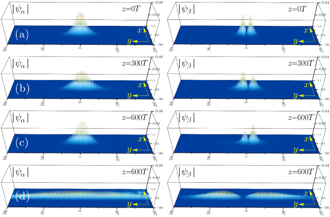
Figure 5: Propagation of dipole topological quasi-soliton in equivalent vector Eq. (3) in nonlinear medium (a)-(c) and its diffraction in linear regime (d). Left column shows $\left|{{\psi}_{\alpha}}\right|$, while right column shows $\left|{{\psi}_{\beta}}\right|$. Parameters are the same as in Fig. 4.

When the combination of two modes ${{\psi}_{\alpha}}$ and ${{\psi}_{\beta}}$ with different propagation constants (i.e., a total field of the form $\psi\sim{{\psi}_{\alpha}}+{{\psi}_{\beta}}$) is substituted into (1), one can formally reduce it to two purely nonlinearly coupled 2D NLS equations by collecting terms $\sim{{e}^{i{{b}_{\alpha k}}z}},{{e}^{i{{b}_{\beta k}}z}}$ and dropping the oscillating terms $\sim{{e}^{i({{b}_{\alpha k}}-{{b}_{\beta k}})z}}$ (thus, accounting only for self- and cross-phase modulation interactions and skipping four-wave mixing terms), without averaging over helix period $T$:

$$\begin{split}i\frac{\partial{{\psi}_{\alpha,\beta}}}{\partial z}=&-\frac{1}{2}{{\Delta}_{\bot}}{{\psi}_{\alpha,\beta}}-\mathcal{R}(\mathbf{r},z){{\psi}_{\alpha,\beta}}\\ &\qquad-({{\left|{{\psi}_{\alpha,\beta}}\right|}^{2}}+2{{\left|{{\psi}_{\beta,\alpha}}\right|}^{2}}){{\psi}_{\alpha,\beta}}\,.\end{split}$$ (3)

The advantage of such a reduction is that (3) allows to follow the evolution of each component. This reduction is partially justified due to rapid variation of phase difference $({{b}_{\alpha k}}-{{b}_{\beta k}})z$ between modes, but it has to be tested numerically because the scale ${{({{b}_{\alpha k}}-{{b}_{\beta k}})}^{-1}}>T$ is not the smallest one in the Floquet system. The model (3) can be also directly derived for two waves with different polarizations/wavelengths. The propagation of the dipole FS in the vector model (3) with a helical kagome array is illustrated in Fig. 5(a)-(c). Indeed, it shows metastable propagation of the dipole soliton, qualitatively similar to the dynamics encountered in the scalar model (Fig. 4). Also, the aforementioned oscillations of the dipole component at the equivalent distances closely match the oscillations of the corresponding projections in Fig. 4 (notice the different direction of the $y$-axis in panels with projections). As in the scalar model, switching-off nonlinearity causes strong diffraction (see Appendix C for the evolution of the peak amplitudes in the linear and nonlinear cases). The remarkable similarity between the dynamics in the scalar model (1) and in the vector model (3) shows that the periodic modulation of the array does not introduce any linear coupling of the involved modes.

In conclusion, we uncovered a new type of topological dipole FS, which is constructed using envelopes featuring the different symmetries imposed on two edge states from different topological gaps exhibiting equal group velocities. The solitonic nature of the wavepackets is consistent with their bifurcation from the linear Floquet-Bloch eigenstates at small amplitudes and by the preservation of their shape over extremely long propagation distances. Our prediction has broad implications, as dipole solitons can be observed for other types of Floquet insulators featuring at least two topological gaps, such as, e.g., Floquet Lieb insulators. It is plausible that more complex multicomponent solitons of non- fundamental nature may be also found. Finally, we anticipate that the reported results may be relevant for polaritonic and atomic nonlinear systems, where topological edge solitons can be sustained by different physical mechanisms.

Appendix A Derivation of model (2) from the main text

Here we provide the detailed derivation of the coupled mode model, equation (2) of the main text (see also R40 ). We start with the model (1) from the main text rewritten as follows

$$i\frac{\partial\psi}{\partial z}=H_{0}({\bm{r}},z)\psi-|\psi|^{2}\psi,$$ (4)

where ${\bm{r}}={\bf i}x+{\bf j}y$,

$$\quad H_{0}=-\frac{1}{2}\nabla^{2}-\mathcal{R}({\bm{r}},z)$$ (5)

and the following properties hold

$$\mathcal{R}({\bm{r}},z)=\mathcal{R}({\bm{r}},z+T)=\mathcal{R}({\bm{r}}+L{\bf j},z)$$ (6)

with $T={2\pi}/{\omega}$, and other notations from the main text.

A.1 The linear problem

Consider the linear problem

$$i\frac{\partial\tilde{\psi}}{\partial z}=H_{0}\tilde{\psi}$$ (7)

(hereafter, tildes stand to distinguish solutions of the linear problem from their nonlinear counterparts, i.e., $\tilde{\psi}$ is the linear limit of $\psi$). A general Floquet-Bloch state (FBS) $\tilde{\psi}({\bm{r}},z)$ satisfies the Floquet (with respect to $z$) and Bloch (with respect to $y$) theorems and allows the representation

$$\tilde{\psi}_{\nu k}({\bm{r}},z)=\phi_{\nu k}({\bm{r}},z)e^{i\tilde{b}_{\nu}(k)z}=u_{\nu k}({\bm{r}},z)e^{iky+i\tilde{b}_{\nu}(k)z},$$ (8)

where $k\in[-K/2,K/2]$ with $K=2\pi/L$ is the Bloch vector along $y-$direction, $\tilde{b}_{\nu}(k)\in[-\omega/2,\omega/2]$, and

$$u_{\nu k}(y,z)=u_{\nu k}(y+L,z)=u_{\nu k}(y,z+T)$$ (9)

(to abbreviate notations we do not show $x-$dependence of $u_{\nu k}$ explicitly). The index $\nu$ stands either for a spatial band or for a topological branch connecting the neighbour gaps at a given edge.

Now equation (7) can be rewritten in terms of the functions $\phi_{\nu k}(y,z)$ and $u_{\nu k}(y,z)$:

$$i\frac{\partial\phi_{\nu k}}{\partial z}-\tilde{b}_{\nu}(k)\phi_{\nu k}=H_{0}\phi_{\nu k}$$ (10)

and

$$i\frac{\partial u_{\nu k}}{\partial z}-\tilde{b}_{\nu}(k)u_{\nu k}=H_{k}u_{\nu k}\,,$$ (11)

where

$$H_{k}=\frac{1}{2}\left(\frac{1}{i}\frac{\partial}{\partial y}+k\right)^{2}-\frac{1}{2}\frac{\partial^{2}}{\partial x^{2}}+\mathcal{R}({\bm{r}},z).$$ (12)

Let the lattice has dimensions defined by $x\in[-\ell_{x},\ell_{x}]$ and $y\in[-\ell_{y},\ell_{y}]$. Let also $\psi$ is subject to the cyclic boundary conditions with respect to $y$ and zero boundary conditions with respect to $x$ (these conditions were also used in numerical simulations):

$$\psi({\bm{r}},z)=\psi({\bm{r}}+2\ell_{y}{\bf j},z),\quad\psi(\pm\ell_{x}{\bf i}+y{\bf j},z)=0.$$ (13)

Respectively, $S=[-\ell_{x},\ell_{x}]\times[-\ell_{y},\ell_{y}]$ is the total area of the lattice. We are interested in the limit where $\ell_{x},\ell_{y}\gg L$ (formally $\ell_{x},\ell_{y}\to\infty$).

Define of the inner products

$$(f(\cdot,z),g(\cdot,z)):=\int_{S}f^{*}({\bm{r}},z)g({\bm{r}},z)d{\bm{r}}$$ (14)

and the $T-$average

$$\langle f\rangle_{T}:=\frac{1}{T}\int_{0}^{T}f({\bm{r}},z)dz.$$ (15)

We emphasize that the inner product in (14) is considered between two functions at the same instant. Below we use only such products and therefore drop the explicit argument $z$, writing $(f(\cdot,z),g(\cdot,z))=(f,g)$.

The following simple properties hold:

Lemma 1

The spectrum $\tilde{b}_{\nu}(k)$ is real.

Proof: Using (10) compute

$$i\left(\phi_{\nu k},\frac{\partial\phi_{\nu k}}{\partial z}\right)-\tilde{b}_{\nu}(k)(\phi_{\nu k},\phi_{\nu k})=(\phi_{\nu k},H_{0}\phi_{\nu k}).$$

The complex conjugate of this equation reads

$$-i\left(\frac{\partial\phi_{\nu k}}{\partial z},\phi_{\nu k}\right)-\tilde{b}_{\nu}^{*}(k)(\phi_{\nu k},\phi_{\nu k})=(\phi_{\nu k},H_{0}\phi_{\nu k}),$$

where we used that $H_{0}$ is Hermitian in the Hilbert space with the inner product (14). Subtracting one of this equation from another and applying the $T$-averaging we obtain

$$i\Big{\langle}\frac{\partial}{\partial z}(\phi_{\nu k},\phi_{\nu k})\Big{\rangle}_{T}=[\tilde{b}_{\nu}(k)-\tilde{b}_{\nu}^{*}(k)]\langle(\phi_{\nu k},\phi_{\nu k})\rangle_{T}\,.$$ (16)

By the $T$-periodicity of $\phi_{\nu k}$, the l.h.s. is zero, and hence $\tilde{b}_{\nu}(k)=\tilde{b}_{\nu}^{*}(k)$.  $\Box$

Lemma 2

Non-degenerate states $\phi_{\nu^{\prime}k^{\prime}}({\bm{r}},z)$ and $\phi_{\nu k}({\bm{r}},z)$, with $(\nu,k)\neq(\nu^{\prime},k^{\prime})$, considered at the same instant $z$, are orthogonal for all $z\geq 0$.

Proof: Using (10) compute

$$i\left(\phi_{\nu^{\prime}k^{\prime}},\frac{\partial\phi_{\nu k}}{\partial z}\right)-\tilde{b}_{\nu}(k)(\phi_{\nu^{\prime}k^{\prime}},\phi_{\nu k})=(\phi_{\nu^{\prime}k^{\prime}},H_{0}\phi_{\nu k})$$ (17)

and

$$i\left(\phi_{\nu k},\frac{\partial\phi_{\nu^{\prime}k^{\prime}}}{\partial z}\right)-\tilde{b}_{\nu^{\prime}}(k^{\prime})(\phi_{\nu k},\phi_{\nu^{\prime}k^{\prime}})=(\phi_{\nu k},H_{0}\phi_{\nu^{\prime}k^{\prime}}).$$ (18)

The complex conjugation of the last equation reads

$$-i\left(\frac{\partial\phi_{\nu^{\prime}k^{\prime}}}{\partial z},\phi_{\nu k}\right)-\tilde{b}_{\nu^{\prime}}(k^{\prime})(\phi_{\nu^{\prime}k^{\prime}},\phi_{\nu k})=(\phi_{\nu^{\prime}k^{\prime}},H_{0}\phi_{\nu k}).$$ (19)

Subtracting (19) from (17), we obtain

$$i\frac{d}{dz}\left(\phi_{\nu^{\prime}k^{\prime}},\phi_{\nu k}\right)+[\tilde{b}_{\nu}(k)-\tilde{b}_{\nu^{\prime}}(k^{\prime})](\phi_{\nu^{\prime}k^{\prime}},\phi_{\nu k})=0.$$ (20)

This is a first order ODE for the inner product $\left(\phi_{\nu^{\prime}k^{\prime}},\phi_{\nu k}\right)$ as a function of $z$, and by assumption of non-degeneracy $\tilde{b}_{\nu}(k)\neq\tilde{b}_{\nu^{\prime}}(k^{\prime})$. Thus, if

$$\left(\phi_{\nu^{\prime}k^{\prime}},\phi_{\nu k}\right)=0$$ (21)

at $z=0$, then this property holds for all $z\geq 0$.

To complete the proof we notice that for a given fixed $z$, in particular for $z=0$ the Hamiltonian $H_{0}$ is Hermitian, and thus (21) holds.  $\Box$

For the next consideration we notice the property, valid for the states from the different bands (of branches) $\nu$ and $\nu^{\prime}$ but equal Bloch wavenumbers $k=k^{\prime}$:

$$\left(\phi_{\nu^{\prime}k}(\cdot,z),\phi_{\nu k}(\cdot,z)\right)=\left(u_{\nu^{\prime}k}(\cdot,z),u_{\nu k}(\cdot,z)\right).$$ (22)

We emphasize that the states $u_{\nu^{\prime}k}^{*}({\bm{r}},z)$ and $u_{\nu k}({\bm{r}},z)$ are considered here at the same instant $z$

By Lemma 2, for $\nu\neq\nu^{\prime}$ and the same instant $z$, $\left(u_{\nu^{\prime}k},u_{\nu k}\right)=0$, while for $\nu=\nu^{\prime}$ this inner product is a constant (independent on $z$). Thus, we can impose the normalization

$$\left(u_{\nu^{\prime}k}(\cdot,z),u_{\nu k}(\cdot,z)\right)=\delta_{\nu\nu^{\prime}}\,.$$ (23)

This condition will be used in what follows.

A.2 The ${\bm{k}}\cdot{\bm{p}}$ perturbation theory

Now we extend the standard ${\bm{k}}\cdot{\bm{p}}$ perturbation theory R67 to the case of $z-$dependent topological FBSs. Let $\tilde{\psi}_{\nu k}({\bm{r}},z)$ be a topological FBS. Consider also a FBS belonging to the same branch $\nu$ but having a Bloch wavevector $k_{1}=k+\delta k$ where $\delta k$ is infinitesimal. Taylor expansion of the dispersion relation yields

$$\tilde{b}_{\nu}(k+\delta k)=\tilde{b}_{\nu}(k)+\tilde{b}_{\nu}^{\prime}(k)\delta k+\frac{1}{2}\tilde{b}_{\nu}^{\prime\prime}(k)(\delta k)^{2}+\cdots$$ (24)

(here a prime stands for the derivative with respect to $k$). On the other hand, equation for $u_{\nu k_{1}}({\bm{r}},z)$ can be rewritten as

$$i\frac{\partial u_{\nu k_{1}}}{\partial z}-\tilde{b}_{\nu}(k_{1})u_{\nu k_{1}}=H_{k}u_{\nu k^{\prime}}+H^{(1)}u_{\nu k_{1}}\delta k+\frac{1}{2}u_{\nu k_{1}}(\delta k)^{2},$$ (25)

where

$$H^{(1)}=\frac{1}{i}\frac{\partial}{\partial y}+k.$$ (26)

Now we compute $\tilde{b}_{\nu}(k_{1})$ and $u_{\nu k_{1}}$ perturbatively from (24), (25) and (26). To this end, we look for a solution in the form of the expansion

$$u_{\nu k_{1}}=u_{\nu k}+\delta k\,u_{\nu k}^{(1)}+(\delta k)^{2}u_{\nu k}^{(2)}+\cdots\;,$$ (27)

where $u_{\nu k}^{(1,2)}$ can be expanded over the complete set of the states $u_{\nu k}$

$$u_{\nu k}^{(j)}=\sum_{\lambda}c_{\nu\lambda}^{(j)}(z)u_{\lambda k}\,,\qquad j=1,2$$ (28)

(notice that the expansion coefficients $c_{\nu\lambda}^{(j)}(z)$ are functions of $z$).

Several important comments are in order.

First, like in the stationary case (see, e.g., R68 ) it is enough to consider only projections of $u_{\nu k}^{(1,2)}$ on the eigenstates with the same Bloch vector $k$, and therefore the sum in (28) is over band number only (this is confirmed by the self-consistency of the expansion). Also this is the reason why the expansion coefficients $c(z)$ are not labeled by the index $k$: they all correspond to the chosen $k$.

Second. Unlike in the stationary perturbation theory, where the sum excludes also the state $u_{\nu k}({\bm{r}},z)$ to which the perturbation $u_{\nu k}^{(1,2)}({\bm{r}},z)$ is orthogonal, now we have to keep this term because the orthogonality (21) is verified only for the same instants $z$, while two states considered at different instants, say at $z_{1}$ and $z_{2}$ such that $z_{1}\neq z_{2}$, are, generally speaking, non-orthogonal. Physically, this means that the mode $u_{\nu k}({\bm{r}},z)$ can be excited at $z=z_{2}$ even if at the instant $z=z_{1}$ it is zero.

Third, the functions $u_{\nu k}^{(1,2)}({\bm{r}},z)$ are $T-$periodic along $z$. This implies that the expansion coefficients $c_{\nu\lambda}^{(j)}(z)$ are also periodic functions of $z$, i.e.,

$$c_{\nu\lambda}^{(j)}(z+T)=c_{\nu\lambda}^{(j)}(z).$$ (29)

Substituting (24), (27), and (28) into (25), collecting terms up to $(\delta k)^{2}$ order, taking into account that the states $u_{\nu k}$ solve Eq. (11), and separating the orders $\delta k$ and $(\delta k)^{2}$ we obtain

$$i\sum_{\lambda}\dot{c}_{\nu\lambda}^{(1)}u_{\lambda k}-\sum_{\lambda}(\tilde{b}_{\nu}-\tilde{b}_{\lambda})c_{\nu\lambda}^{(1)}u_{\lambda k}-\tilde{b}_{\nu}^{\prime}u_{\nu k}=H^{(1)}u_{\nu k}\,,$$ (30)

$$i\sum_{\lambda}\dot{c}_{\nu\lambda}^{(2)}u_{\lambda k}-\sum_{\lambda}(\tilde{b}_{\nu}-\tilde{b}_{\lambda})c_{\nu\lambda}^{(2)}u_{\lambda k}-\tilde{b}_{\nu}^{\prime}\sum_{\lambda}c_{\nu\lambda}^{(1)}u_{\lambda k}-\frac{1}{2}\tilde{b}_{\nu}^{\prime\prime}u_{\nu k}=H^{(1)}\sum_{\lambda}c_{\nu\lambda}^{(1)}u_{\lambda k}+\frac{1}{2}u_{\nu k}\,,$$ (31)

where the overdot stands for the derivative with respect to $z$: $\dot{c}=dc/dz$.

Applying $(u_{\nu k},\cdot)$ to (30) we obtain

$$i\frac{dc_{\nu\nu}^{(1)}}{dz}-\tilde{b}_{\nu}^{\prime}=(u_{\nu k},H^{(1)}u_{\nu k}).$$ (32)

By the requirement (29) $\langle dc_{\nu\nu}^{(j)}/dz\rangle_{T}=0$ and hence

$$\tilde{b}_{\nu}^{\prime}(k)=-\langle(u_{\nu k},H^{(1)}u_{\nu k})\rangle_{T}\,.$$ (33)

We rewrite this expression as

$$v_{\nu}(k)=-\tilde{b}_{\nu}^{\prime}(k)=\left\langle\left(\phi_{\nu k},\frac{1}{i}\frac{\partial}{\partial y}\phi_{\nu k}\right)\right\rangle_{T}$$ (34)

(bellow we argue that $v_{\nu}(k)$ represents the group velocity).

In the absence of resonances, the $T-$periodic solution of (32) satisfying zero initial condition, $c_{\nu\nu}^{(1)}(0)=0$ reads

$$c_{\nu\nu}^{(1)}(z)=\frac{1}{i}\int_{0}^{z}\left[h_{\nu\nu}(z^{\prime})-\langle h_{\nu\nu}\rangle_{T}\right]dz^{\prime},$$ (35)

where we defined a $T-$periodic function

$$h_{\nu\lambda}(z+T)=h_{\nu\lambda}(z):=\left(\phi_{\nu k},\frac{1}{i}\frac{\partial}{\partial y}\phi_{\lambda k}\right),$$ (36)

thus ensuring the equality

$$\int_{0}^{T}\left[h_{\nu\lambda}(z^{\prime})-\langle h_{\nu\lambda}\rangle_{T}\right]dz^{\prime}=0.$$ (37)

Applying $(u_{\lambda k},\cdot)$ to (30) we obtain the differential equations for $c_{\nu\lambda}^{(1)}(z)$ ($\lambda\neq\nu$)

$$i\dot{c}_{\nu\lambda}^{(1)}-\Delta_{\nu\lambda}c_{\nu\lambda}^{(1)}=h_{\nu\lambda}^{*}(z),\quad\Delta_{\nu\lambda}=\tilde{b}_{\nu}-\tilde{b}_{\lambda}\,.$$ (38)

Recalling (36) and using the Fourier expansion

$$h_{\nu\lambda}^{*}(z)=\sum_{m}h_{\nu\lambda}^{(m)}e^{-if_{m}z},\qquad f_{m}=2\pi\frac{m}{T}.$$ (39)

the $T-$periodic solution of (38) can be written as

$$c_{\nu\lambda}^{(1)}(z)=\sum_{m}\frac{h_{\nu\lambda}^{(m)}}{f_{m}-\Delta_{\nu\lambda}}e^{-if_{m}z}.$$ (40)

We notice that generally speaking $c_{\nu\lambda}^{(1)}(0)\neq 0$.

Now we turn to the equation appearing in the second order:

$$\frac{1}{2}\tilde{b}_{\nu}^{\prime\prime}=i\dot{c}_{\nu\nu}^{(2)}-\tilde{b}_{\nu}^{\prime}c_{\nu\nu}^{(1)}-\sum_{\lambda}(u_{\nu k},H^{(1)}u_{\lambda k})c_{\nu\lambda}^{(1)}-\frac{1}{2}\,.$$ (41)

Notice that $c_{\nu\lambda}^{(j)}$ does not depend on $y$ while $H^{(1)}$ acts on the functions of $y$. Since $\tilde{b}_{\nu}^{\prime\prime}$ is a constant, and all coefficients $c_{\nu\nu^{\prime}}^{(j)}$ are $T-$periodic, the easiest wave to obtain $\tilde{b}_{\nu}^{\prime\prime}$ is to perform $T-$averaging. This gives

$$\frac{1}{2}\tilde{b}_{\nu}^{\prime\prime}=-\frac{1}{2}-\sum_{\lambda\neq\nu}\left\langle(u_{\nu k},H^{(1)}u_{\lambda k})c_{\nu\lambda}^{(1)}\right\rangle_{T}\,,$$ (42)

where we have taken into account (33). Comparing this with (24) and returning to the FBSs we obtain the final form of the dispersion of the group velocity (the effective diffraction coefficient)

$$\tilde{b}_{\nu}^{\prime\prime}(k)=-1-2\sum_{\lambda\neq\nu}\left\langle h_{\nu\lambda}c_{\nu\lambda}^{(1)}\right\rangle_{T}\,.$$ (43)

A.3 Multiple-scale expansion

Now we apply the multiple-scale expansion to the nonlinear problem (4). To this end, we use two sets of scaled variables

$$(y_{0},y_{1},y_{2}...):=(y,\mu y,\mu^{2}y,...),$$ (44)

$$(z_{0},z_{1},z_{2}...):=(z,\mu z,\mu^{2}z,...),$$ (45)

where $\mu\ll 1$ is a formal small parameter. The scaled variables are treated as independent. Respectively we have

$$H_{0} = \tilde{H}_{0}+\mu\tilde{H}^{(1)}+\mu^{2}\tilde{H}^{(2)},$$ (46)

$$\tilde{H}^{(1)} = -\frac{\partial^{2}}{\partial y_{0}\partial y_{1}},$$ (47)

$$\tilde{H}^{(2)} = -\frac{\partial^{2}}{\partial y_{0}\partial y_{2}}-\frac{1}{2}\frac{\partial^{2}}{\partial y_{1}^{2}},$$ (48)

where $\tilde{H}_{0}$ is $H_{0}$ with the substitution $y\to y_{0}$. We also have

$$\frac{\partial}{\partial z}=\frac{\partial}{\partial z_{0}}+\mu\frac{\partial}{\partial z_{1}}+\mu^{2}\frac{\partial}{\partial z_{2}}+\cdots\;.$$ (49)

In this work we are interested in evolution of two nonlinearly coupled modes having the same Bloch vector $k$ but belonging to different branches denoted as $\nu=\alpha$ and $\nu=\beta$ (see Fig. 1 in the main text). Respectively, we look for a solution of (4) in the form

$$\psi =\mu\left[A_{\alpha}(y_{1},z_{1})\phi_{\alpha k}e^{i\tilde{b}_{\alpha}z}+A_{\beta}(y_{1},z_{1})\phi_{\beta k}e^{i\tilde{b}_{\beta}z}\right]$$

$$+\mu^{2}\left[\phi_{\alpha}^{(1)}e^{i\tilde{b}_{\alpha}z}+\phi_{\beta}^{(1)}e^{i\tilde{b}_{\beta}z}\right]$$

$$+\mu^{3}\left[\phi_{\alpha}^{(2)}e^{i\tilde{b}_{\alpha}z}+\phi_{\beta}^{(2)}e^{i\tilde{b}_{\beta}z}\right]$$

$$+\cdots\;.$$ (50)

Here $A_{\alpha}$ and $A_{\beta}$ are slowly varying envelopes of the states $\phi_{\alpha k}$ and $\phi_{\beta k}$; in the arguments of $A_{\alpha,\beta}$ only the most rapid variables are indicated, e.g., $A(y_{1},z_{1})$ stands for $A(y_{1},,y_{2},...;z_{1},z_{2},...)$. To shorten notations further we do not show $k$ in the arguments of $\tilde{b}_{\alpha}$ and $\tilde{b}_{\beta}$.

At each instant $z_{0}$, the second and third order corrections in (A.3) can be expanded as follows

$$\phi_{\alpha}^{(j)}=\sum_{\nu}B_{\alpha\nu}^{(j)}(x_{1},z_{0})\phi_{\nu k}(z_{0}),$$ (51a)

$$\phi_{\beta}^{(j)}=\sum_{\nu}B_{\beta\nu}^{(j)}(x_{1},z_{0})\phi_{\nu k}(z_{0}).$$ (51b)

Now we substitute (A.3) into (4) considered in the scaled variables. In the first order of $\mu$, the obtained equation is identically satisfied.

A.3.1 Order $\mu^{2}$

In the second order we obtain

$$\left[i\frac{\partial A_{\alpha}}{\partial z_{1}}\phi_{\alpha k}+i\sum_{\nu}\frac{\partial B_{\alpha\nu}^{(1)}}{\partial z_{0}}\phi_{\nu k}+i\sum_{\nu}B_{\alpha\nu}^{(1)}\frac{\partial\phi_{\nu k}}{\partial z_{0}}-\tilde{b}_{\alpha}\sum_{\nu}B_{\alpha\nu}^{(1)}\phi_{\nu k}\right]e^{i\tilde{b}_{\alpha}z}$$

$$+\left[i\frac{\partial A_{\beta}}{\partial z_{1}}\phi_{\beta k}+i\sum_{\nu}\frac{\partial B_{\beta\nu}^{(1)}}{\partial z_{0}}\phi_{\nu k}+i\sum_{\nu}B_{\beta\nu}^{(1)}\frac{\partial\phi_{\nu k}}{\partial z_{0}}-\tilde{b}_{\beta}\sum_{\nu}B_{\beta\nu}^{(1)}\phi_{\nu k}\right]e^{i\tilde{b}_{\beta}z}$$

$$=\left[\tilde{H}_{0}\sum_{\nu}B_{\alpha\nu}^{(1)}\phi_{\nu k}+\tilde{H}^{(1)}A_{\alpha}\phi_{\alpha k}\right]e^{i\tilde{b}_{\alpha}z}+\left[\tilde{H}_{0}\sum_{\nu}B_{\beta\nu}^{(1)}\phi_{\nu k}+\tilde{H}^{(1)}A_{\beta}\phi_{\beta k}\right]e^{i\tilde{b}_{\beta}z}.$$ (52)

Collecting the terms $\propto e^{i\tilde{b}_{\alpha}z}$ and $\propto e^{i\tilde{b}_{\beta}z}$ separately, using (10) with $H_{0}$ replaced by $\tilde{H}_{0}$ with $\nu=\alpha$ and $\nu=\beta$, and using the explicit expression for $\tilde{H}_{1}$ we rewrite (A.3.1) in the form of two equations as follows

$$i\frac{\partial A_{\alpha}}{\partial z_{1}}\phi_{\alpha k}+i\sum_{\nu}\frac{\partial B_{\alpha\nu}^{(1)}}{\partial z_{0}}\phi_{\nu k}-\sum_{\nu}(\tilde{b}_{\alpha}-\tilde{b}_{\nu})B_{\alpha\nu}^{(1)}\phi_{\nu k}=-\frac{\partial A_{\alpha}}{\partial y_{1}}\frac{\partial\phi_{\alpha k}}{\partial y_{0}},$$ (53a)

$$i\frac{\partial A_{\beta}}{\partial z_{1}}\phi_{\beta k}+i\sum_{\nu}\frac{\partial B_{\beta\nu}^{(1)}}{\partial z_{0}}\phi_{\nu k}-\sum_{\nu}(\tilde{b}_{\beta}-\tilde{b}_{\nu})B_{\beta\nu}^{(1)}\phi_{\nu k}=-\frac{\partial A_{\beta}}{\partial x_{1}}\frac{\partial\phi_{\beta k}}{\partial y_{0}}.$$ (53b)

Now we apply $(\phi_{\alpha k},\cdot)$ to (53a) to obtain

$$i\frac{\partial A_{\alpha}}{\partial z_{1}}+i\left(\psi_{\alpha k},\frac{1}{i}\frac{\partial}{\partial y_{0}}\psi_{\alpha k}\right)\frac{\partial A_{\alpha}}{\partial y_{1}}+\frac{\partial B_{\alpha\alpha}^{(1)}}{\partial z_{0}}=0,$$ (54)

where we have used

$$\left(\phi_{\nu k},\frac{1}{i}\frac{\partial}{\partial y_{0}}\phi_{\alpha k}\right)\equiv\left(\psi_{\nu k},\frac{1}{i}\frac{\partial}{\partial y_{0}}\psi_{\alpha k}\right).$$ (55)

Taking into account that all terms in (54) are $T-$periodic with respect to $z_{0}$, we average (54) over the period $T$ to obtain

$$\frac{\partial A_{\alpha}}{\partial z_{1}}+v_{\alpha}\frac{\partial A_{\alpha}}{\partial y_{1}}=0,$$ (56)

where the group velocity $v_{\alpha}$ is given by (34). Analogously from (53b) we obtain

$$\frac{\partial A_{\beta}}{\partial z_{1}}+v_{\beta}\frac{\partial A_{\beta}}{\partial y_{1}}=0.$$ (57)

An important property, is used in the main text, is the equality of the group velocities of the chosen modes, i.e.,

$$v_{\alpha}=v_{\beta}=v.$$ (58)

This means that both $A_{\alpha}$ and $A_{\beta}$ depend on the “fast variables” $z_{1}$ and $y_{1}$ only through the combination $Y=y_{1}-vz_{1}$:

$$A_{\alpha,\beta}\equiv A_{\alpha,\beta}(Y;z_{2},x_{2}).$$ (59)

We also obtain

$$B_{\alpha\alpha}^{(1)}=-i\frac{\partial A_{\alpha}}{\partial y_{1}}c_{\alpha\alpha}^{(1)}\;,\quad B_{\beta\beta}^{(1)}=-i\frac{\partial A_{\beta}}{\partial y_{1}}c_{\beta\beta}^{(1)}\,,$$ (60)

where $c_{\nu\nu}^{(1)}$ is defined in (35). Importantly, at this stage we assume that the modes are non-resonant, i.e., no zero denominators appear in (35).

For $\nu\neq\alpha$ we apply $(\phi_{\nu k},\cdot)$ to (53a) and obtain [cf. (38)]

$$i\frac{\partial B_{\alpha\nu}^{(1)}}{\partial z_{0}}-(\tilde{b}_{\alpha}-\tilde{b}_{\nu})B_{\alpha\nu}^{(1)}=-i\frac{\partial A}{\partial y_{1}}h_{\alpha\nu}^{*}(z_{0}).$$ (61)

Its $T-$ periodic solution is found as

$$B_{\alpha\nu}^{(1)}(z_{0})=-i\frac{\partial A_{\alpha}}{\partial y_{1}}c_{\alpha\nu}^{(1)}\,,$$ (62)

where $c_{\alpha\nu}^{(1)}$ is defined in (40). Similarly, for the $\beta-$component we obtain

$$B_{\beta\nu}^{(1)}(z_{0})=-i\frac{\partial A_{\beta}}{\partial y_{1}}c_{\beta\nu}^{(1)}\,.$$ (63)

A.3.2 Order $\mu^{3}$

Turning to the equations of the $\mu^{3}$ order we write them already separated for the terms $\propto e^{i\tilde{b}_{\alpha}z}$ and $\propto e^{i\tilde{b}_{\beta}z}$, where all entries $\propto e^{\pm 3i\tilde{b}_{\alpha}z}$ and $\propto e^{\pm 3i\tilde{b}_{\beta}z}$ are dropped:

$$i\frac{\partial A_{\alpha}}{\partial z_{2}}\phi_{\alpha k}+i\sum_{\nu}\frac{\partial B_{\alpha\nu}^{(2)}}{\partial z_{0}}\phi_{\nu k}+i\sum_{\nu}\frac{\partial B_{\alpha\nu}^{(1)}}{\partial z_{1}}\phi_{\nu k}+i\sum_{\nu}B_{\alpha\nu}^{(2)}\frac{\partial\phi_{\nu k}}{\partial z_{0}}-\tilde{b}_{\alpha}\sum_{\nu}B_{\alpha\nu}^{(2)}\phi_{\nu k}$$

$$=\tilde{H}_{0}\sum_{\nu}B_{\alpha\nu}^{(2)}\phi_{\nu k}+\tilde{H}_{1}\sum_{\nu}B_{\alpha\nu}^{(1)}\phi_{\nu k}+H_{2}A_{\alpha}\phi_{\alpha k}-|A_{\alpha}|^{2}A_{\alpha}|\phi_{\alpha k}|^{2}\phi_{\alpha k}-2|A_{\beta}|^{2}A_{\alpha}|\phi_{\beta k}|^{2}\phi_{\alpha k}\,,$$ (64)

$$i\frac{\partial A_{\beta}}{\partial z_{2}}\phi_{\alpha k}+i\sum_{\nu}\frac{\partial B_{\beta\nu}^{(2)}}{\partial z_{0}}\phi_{\nu k}+i\sum_{\nu}\frac{\partial B_{\beta\nu}^{(1)}}{\partial z_{1}}\phi_{\nu k}+i\sum_{\nu}B_{\beta\nu}^{(2)}\frac{\partial\phi_{\nu k}}{\partial z_{0}}-\tilde{b}_{\beta}\sum_{\nu}B_{\beta\nu}^{(2)}\phi_{\nu k}$$

$$=\tilde{H}_{0}\sum_{\nu}B_{\beta\nu}^{(2)}\phi_{\nu k}+\tilde{H}^{(1)}\sum_{\nu}B_{\alpha\nu}^{(1)}\phi_{\nu k}+\tilde{H}^{(2)}A_{\beta}\phi_{\beta k}-|A_{\beta}|^{2}A_{\beta}|\phi_{\beta k}|^{2}\phi_{\beta k}-2|A_{\alpha}|^{2}A_{\beta}|\phi_{\alpha k}|^{2}\phi_{\beta k}\,.$$ (65)

Projecting (A.3.2) and (A.3.2) to $\phi_{\alpha k}$ and $\phi_{\beta k}$ respectively we obtain

$$i\frac{\partial A_{\alpha}}{\partial z_{2}}+i\frac{\partial B_{\alpha\alpha}^{(2)}}{\partial z_{0}}+i\frac{\partial B_{\alpha\alpha}^{(1)}}{\partial z_{1}}=-\sum_{\nu}\frac{\partial B_{\alpha\nu}^{(1)}}{\partial y_{1}}\left(\phi_{\alpha k},\frac{\partial\phi_{\alpha k}}{\partial y_{0}}\right)-\frac{1}{2}\frac{\partial^{2}A_{\alpha}}{\partial y_{1}^{2}}-\frac{\partial A_{\alpha}}{\partial y_{2}}\left(\phi_{\alpha k},\frac{\partial\phi_{\alpha k}}{\partial y_{0}}\right)$$

$$-|A_{\alpha}|^{2}A_{\alpha}(\phi_{\alpha k},|\phi_{\alpha k}|^{2}\phi_{\alpha k})-2|A_{\beta}|^{2}A_{\alpha}(\phi_{\alpha k},|\phi_{\beta k}|^{2}\phi_{\alpha k}),$$ (66)

$$i\frac{\partial A_{\beta}}{\partial z_{2}}+i\frac{\partial B_{\beta\beta}^{(2)}}{\partial z_{0}}+i\frac{\partial B_{\beta\beta}^{(1)}}{\partial z_{1}}=-\sum_{\nu}\frac{\partial B_{\beta\nu}^{(1)}}{\partial y_{1}}\left(\phi_{\beta k},\frac{\partial\phi_{\beta k}}{\partial y_{0}}\right)-\frac{1}{2}\frac{\partial^{2}A_{\beta}}{\partial y_{1}^{2}}-\frac{\partial A_{\beta}}{\partial y_{2}}\left(\phi_{\beta k},\frac{\partial\phi_{\beta k}}{\partial y_{0}}\right)$$

$$-|A_{\beta}|^{2}A_{\beta}(\phi_{\beta k},|\phi_{\beta k}|^{2}\phi_{\beta k})-2|A_{\alpha}|^{2}A_{\beta}(\phi_{\beta k},|\phi_{\alpha k}|^{2}\phi_{\beta k}).$$ (67)

It follows from (62), (56), (57) and (58) that

$$i\frac{\partial B_{\alpha\nu}^{(1)}}{\partial z_{1}}=v\frac{\partial^{2}A_{\alpha}}{\partial y_{1}^{2}}c_{\alpha\nu}^{(1)},\qquad i\frac{\partial B_{\beta\nu}^{(1)}}{\partial z_{1}}=v\frac{\partial^{2}A_{\beta}}{\partial y_{1}^{2}}c_{\beta\nu}^{(1)}\,.$$ (68)

Thus (53a) and (53b) are rewritten as

$$i\frac{\partial A_{\alpha}}{\partial z_{2}}+iv\frac{\partial A_{\alpha}}{\partial y_{2}}+\frac{1}{2}\frac{\partial^{2}A_{\alpha}}{\partial y_{1}^{2}}+i\sum_{\nu\neq\alpha}h_{\alpha\nu}\frac{\partial B_{\alpha\nu}^{(1)}}{\partial y_{1}}+|A_{\alpha}|^{2}A_{\alpha}(\phi_{\alpha k},|\phi_{\alpha k}|^{2}\phi_{\alpha k})+2|A_{\beta}|^{2}A_{\alpha}(\phi_{\alpha k},|\phi_{\beta k}|^{2}\phi_{\alpha k})=-i\frac{\partial B_{\alpha\alpha}^{(2)}}{\partial z_{0}},$$ (69)

$$i\frac{\partial A_{\beta}}{\partial z_{2}}+iv\frac{\partial A_{\beta}}{\partial y_{2}}+\frac{1}{2}\frac{\partial^{2}A_{\beta}}{\partial y_{1}^{2}}+i\sum_{\nu\neq\beta}h_{\beta\nu}\frac{\partial B_{\beta\nu}^{(1)}}{\partial y_{1}}+|A_{\beta}|^{2}A_{\beta}(\phi_{\beta k},|\phi_{\beta k}|^{2}\phi_{\beta k})+2|A_{\beta}|^{2}A_{\alpha}(\phi_{\beta k},|\phi_{\alpha k}|^{2}\phi_{\beta k})=-i\frac{\partial B_{\beta\beta}^{(2)}}{\partial z_{0}}.$$ (70)

Since all terms in this equations are either $z_{0}-$independent or $T-$periodic we average over the period. The last term in (69) and (70) vanish because of the periodicity, while using (62) and (43) we obtain

$$\frac{1}{2}\frac{\partial^{2}A_{\alpha}}{\partial y_{1}^{2}}+i\left\langle\sum_{\nu\neq\alpha}h_{\alpha\nu}\frac{\partial B_{\alpha\nu}^{(1)}}{\partial y_{1}}\right\rangle_{T}$$

$$=\frac{1}{2}\frac{\partial^{2}A_{\alpha}}{\partial y_{1}^{2}}\left(1+2\sum_{\nu\neq\alpha}\left\langle h_{\alpha\nu}c_{{}_{\alpha}\nu}^{(1)}\right\rangle_{T}\right)=-\frac{\tilde{b}_{\alpha}^{\prime\prime}}{2}\frac{\partial^{2}A_{\alpha}}{\partial y_{1}^{2}}.$$ (71)

Similar relation holds for $\alpha$ replaced by $\beta$.

Looking for the envelopes $A_{\alpha}$ and $A_{\beta}$ which are $y_{2}-$independent, we obtain two nonlinearly coupled NLS equations. Setting the formal small parameter $\mu$ to be one, i.e., returning to non-scaled physical variables we obtain

$$i\frac{\partial A_{\alpha}}{\partial z}-\frac{\tilde{b}_{\alpha}^{\prime\prime}}{2}\frac{\partial^{2}A_{\alpha}}{\partial Y^{2}}+\chi_{\alpha}|A_{\alpha}|^{2}A_{\alpha}+2\chi_{\rm x}|A_{\beta}|^{2}A_{\alpha}=0,$$ (72a)

$$i\frac{\partial A_{\beta}}{\partial z}-\frac{\tilde{b}_{\beta}^{\prime\prime}}{2}\frac{\partial^{2}A_{\beta}}{\partial Y^{2}}+\chi_{\beta}|A_{\beta}|^{2}A_{\beta}+2\chi_{\rm x}|A_{\alpha}|^{2}A_{\beta}=0,$$ (72b)

where the nonlinearity coefficients are given by

$$\chi_{\alpha} =\langle(\psi_{\alpha k},|\psi_{\alpha k}|^{2}\psi_{\alpha k})\rangle_{T}\,,$$ (73)

$$\chi_{\beta} =\langle(\psi_{\beta k},|\psi_{\beta k}|^{2}\psi_{\beta k})\rangle_{T}\,,$$ (74)

$$\chi_{\rm x} =\langle(\psi_{\alpha k},|\psi_{\beta k}|^{2}\psi_{\alpha k})\rangle_{T}=\langle(\psi_{\beta k},|\psi_{\alpha k}|^{2}\psi_{\beta k})\rangle_{T}\,.$$ (75)

These are equations (2) from the main text, where $\tilde{b}_{\nu}^{\prime\prime}$ is replaced by $b_{\nu}^{\prime\prime}$ referring to the linear spectrum.

Appendix B Linear stability analysis of system (2)

To perform linear stability analysis in the frames of the envelope equation (2) from the main text we substitute into it the perturbed solution $A_{\nu}=(w_{\nu}+\mu_{\nu}e^{\delta z}+\eta_{\nu}^{*}e^{\delta^{*}z})e^{ib_{\nu}^{\textrm{nl}}z}$, where $\mu_{\nu},\eta_{\nu}$ are small perturbations, $\delta$ is the complex perturbation growth rate, and linearize resulting system. This yields linear eigenvalue problem:

$$i\delta\mu_{\alpha,\beta}=+\frac{b_{\alpha,\beta}^{\prime\prime}}{2}\frac{\partial^{2}\mu_{\alpha,\beta}}{\partial Y^{2}}-\chi_{\alpha,\beta}(2\mu_{\alpha,\beta}+\eta_{\alpha,\beta})w_{\alpha,\beta}^{2}-2\chi_{\textrm{x}}[w_{\beta,\alpha}^{2}\mu_{\alpha,\beta}+w_{\alpha}w_{\beta}(\mu_{\beta,\alpha}+\eta_{\beta,\alpha})]+b_{\alpha,\beta}^{\textrm{nl}}\mu_{\alpha,\beta}\,,$$ (76a)

$$i\delta\eta_{\alpha,\beta}=-\frac{b_{\alpha,\beta}^{\prime\prime}}{2}\frac{\partial^{2}\eta_{\alpha,\beta}}{\partial Y^{2}}+\chi_{\alpha,\beta}(2\eta_{\alpha,\beta}+\mu_{\alpha,\beta})w_{\alpha,\beta}^{2}+2\chi_{\textrm{x}}[w_{\beta,\alpha}^{2}\eta_{\alpha,\beta}+w_{\alpha}w_{\beta}(\eta_{\beta,\alpha}+\mu_{\beta,\alpha})]-b_{\alpha,\beta}^{\textrm{nl}}\eta_{\alpha,\beta}\,.$$ (76b)

Stationary envelopes $w_{\alpha,\beta}$ that enter linear eigenvalue problem [Eqs. (73a) and (73b)] can be found using Newton method from the following system of nonlinearly coupled ordinary differential equations [also obtained from Eq. (2) of the main text]:

$$b_{\alpha}^{\textrm{nl}}w_{\alpha}=-\frac{b_{\alpha}^{\prime\prime}}{2}\frac{\partial^{2}w_{\alpha}}{\partial Y^{2}}+\chi_{\alpha}w_{\alpha}^{3}+2\chi_{\rm x}w_{\beta}^{2}w_{\alpha},$$ (77a)

$$b_{\beta}^{\textrm{nl}}w_{\beta}=-\frac{b_{\beta}^{\prime\prime}}{2}\frac{\partial^{2}w_{\beta}}{\partial Y^{2}}+\chi_{\beta}w_{\beta}^{3}+2\chi_{\rm x}w_{\alpha}^{2}w_{\beta}.$$ (77b)

Linear eigenvalue problem [Eqs. (73a) and (73b)] was solved using standard eigenvalue solver to obtain the dependence of perturbation growth rate $\delta_{\textrm{re}}=\textrm{Re}(\delta)$ on nonlinear propagation constant shifts $b_{\alpha}^{\textrm{nl}}$ and $b_{\beta}^{\textrm{nl}}$ of two soliton components. We identified the most unstable perturbation mode with largest growth rate and plotted it as a function of $b_{\alpha}^{\textrm{nl}}$ for several $b_{\beta}^{\textrm{nl}}$ values in Fig. 3(d) from the main text. One can see, that for nonlinear phase shifts used in the paper (they should be sufficiently small to ensure that the envelope covers many $y$-periods of the array) growth rate for the most unstable perturbation eigenmode is typically very low. Thus, for soliton shown in Fig. 3(b) one has $\delta_{\textrm{re}}=0.00044$. The characteristic propagation distance at which such instability may develop can be estimated as $1/\delta_{\textrm{re}}$ and for all cases considered it exceeds helix period $T$ at least by two orders of magnitude that implies metastability (very long-living character) of the obtained dipole solitons. Due to their metastability, one can observe long-range propagation of dipole solitons along the edge of the insulator without breakup into sets of fundamental solitons. Notice that perturbation growth rate vanishes close to the left border of the existence domain of vector solitons, when $b_{\alpha}^{\textrm{nl}}\to b_{\alpha}^{\textrm{low}}$ , but so does also the dipole component of soliton. Thus, in the paper the optimal situation was chosen, when this component is still considerable in comparison with other bell-shaped component, and at the same time, growth rate $\delta_{\textrm{re}}$ remains very small. The analysis described above guarantees metastability of the one-dimensional envelopes of vector topological edge solitons.

Appendix C Evolution of peak amplitudes in linear and nonlinear regimes

The fact that dipole topological solitons are indeed the objects, sustained by the nonlinearity of the material, becomes especially obvious from comparison of evolution of peak amplitudes of the wavepackets in nonlinear and linear cases. Such a comparison is presented in Fig. 1 below that shows the dependence of the maximal amplitude of the wavepacket propagated in scalar model (1) from the main text [Fig. 1(a), $a=\textrm{max}|\psi|$] and wavepacket, whose components evolve in accordance with vector model (3) [Fig. 1(b), $a_{\alpha,\beta}=\textrm{max}|\psi_{\alpha,\beta}|$]. The amplitude in nonlinear medium is shown with black (in scalar case) or black and red (in vector case) lines. Note that fast oscillations with period $T$ clearly visible in the plots reflect the underlying Floquet nature of the obtained solitons. While in nonlinear case peak amplitude does not decrease notably over considerable distance shown, in linear versions of the above mentioned models, where nonlinearity was deliberately switched off (see green lines), peak amplitude rapidly drops down reflecting strong diffraction broadening observed in Figs. 4(d) and 5(d) from the main text.

Figure 6: Peak amplitude of the dipole soliton versus distance in (a) scalar and (b) vector models corresponding to the dynamics shown in Figs. 4 and 5 from the main text. Black and red curves - peak amplitude in nonlinear regime, green curves – peak amplitude in linear regime.

References

• (1) M. Z. Hasan and C. L. Kane, “Topological insulators,” Rev. Mod. Phys. 82, 3045 (2010).
• (2) X.-L. Qi and S.-C. Zhang, “Topological insulators and superconductors,” Rev. Mod. Phys. 83, 1057 (2011).
• (3) R. Süsstrunk and S. D. Huber, “Observation of phononic helical edge states in a mechanical topological insulator,” Science 349, 47 (2015).
• (4) S. D. Huber, “Topological mechanics,” Nat. Phys. 12, 621 (2016).
• (5) C. He, X. Ni, H. Ge, X.-C. Sun, Y.-B. Chen, M.-H. Lu, X.-P. Liu, and Y.- F. Chen, “Acoustic topological insulator and robust one-way sound transport,” Nat. Phys. 12, 1124 (2016).
• (6) Y. G. Peng, C. Z. Qin, D. G. Zhao, Y. X. Shen, X. Y. Xu, M. Bao, H. Jia, and X. F. Zhu, “Experimental demonstration of anomalous Floquet topological insulator for sound,” Nat. Commun. 7, 13368 (2016).
• (7) G. Jotzu, M. Messer, R. Desbuquois, M. Lebrat, T. Uehlinger, D. Greif, and T. Esslinger, “Experimental realization of the topological Haldane model with ultracold fermions,” Nature 515, 237 (2014).
• (8) N. Goldman, J. Dalibard, A. Dauphin, F. Gerbier, M. Lewenstein, P. Zoller, and I. B. Spielman, “Direct imaging of topological edge states in cold-atom systems,” PNAS, 110, 6736 (2013).
• (9) A. V. Nalitov, D. D. Solnyshkov, and G. Malpuech, “Polariton Z topological insulator,” Phys. Rev. Lett. 114, 116401 (2015).
• (10) P. St-Jean, V. Goblot, E. Galopin, A. Lemaître, T. Ozawa, L. Gratiet, I. Sagnes, J. Bloch, A. Amo, “Lasing in topological edge states of a 1D lattice,” Nat. Photon. 11, 651 (2017).
• (11) S. Klembt, T. H. Harder, O. A. Egorov, K. Winkler, R. Ge, M. A. Bandres, M. Emmerling, L. Worschech, T. C. H. Liew, M. Segev, C. Schneider, and S. Höfling, “Exciton-polariton topological insulator,” Nature 562, 552 (2018).
• (12) F. D. Haldane and S. Raghu, “Possible realization of directional optical waveguides in photonic crystals with broken time-reversal symmetry,” Phys. Rev. Lett. 100, 013904 (2008).
• (13) Z. Wang, Y. Chong, J. D. Joannopoulos, and M. Soljacic, “Observation of unidirectional backscattering-immune topological electro-magnetic states,” Nature 461, 772 (2009).
• (14) M. Hafezi, E. A. Demler, M. D. Lukin, and J. M. Taylor, “Robust optical delay lines with topological protection,” Nat. Phys. 7, 907 (2011).
• (15) A. B. Khanikaev, S. H. Mousavi, W. K. Tse, M. Kargarian, A. H. MacDonald, G. Shvets, “Photonic topological insulators,” Nat. Materials 12, 233 (2013).
• (16) N. H. Lindner, G. Refael, and V. Galitski, “Floquet topological insulator in semiconductor quantum wells,” Nat. Phys. 7, 490 (2011).
• (17) M. C. Rechtsman, J. M. Zeuner, Y. Plotnik, Y. Lumer, D. Podolsky, F. Dreisow, S. Nolte, M. Segev, and A. Szameit, “Photonic Floquet topological insulators,” Nature 496, 196 (2013).
• (18) L. J. Maczewsky, J. M. Zeuner, S. Nolte, and A. Szameit, “Observation of photonic anomalous Floquet topological insulators,” Nat. Commun. 8, 13756 (2017).
• (19) S. Mukherjee, A. Spracklen, M. Valiente, E. Andersson, P. Öhberg, N. Goldman, R. R. Thomson, “Experimental observation of anomalous topological edge modes in a slowly driven photonic lattice,” Nat. Commun. 8, 13918 (2017).
• (20) L. Lu, J. D. Joannopoulos, and M. Soljačić, “Topological photonics,” Nat. Photon. 8, 821 (2014).
• (21) T. Ozawa, H. M. Price, A. Amo, N. Goldman, M. Hafezi, L. Lu, M. C. Rechtsman, D. Schuster, J. Simon, O. Zilberberg, I. Carusotto, “Topological photonics,” Rev. Mod. Phys. 91, 015006 (2019).
• (22) M. Kim, Z. Jacob, and J. Rho, “Recent advances in 2D, 3D and higher- order topological photonics,” Light: Science & Applications 9, 130 (2020).
• (23) D. Smirnova, D. Leykam, Y. D. Chong, and Y. Kivshar, “Nonlinear topological photonics,” Appl. Phys. Rev. 7, 021306 (2020).
• (24) Y. Ota, K. Takata, T. Ozawa, A. Amo, Z. Jia, B. Kante, M. Notomi, Y. Arakawa, S. Iwamoto, “Active topological photonics,” Nanophotonics 9, 547 (2020).
• (25) S. Rachel, “Interacting topological insulators: A review,” Reports Prog. Phys. 81, 116501 (2018).
• (26) D. Leykam and Y. D. Chong, “Edge solitons in nonlinear-photonic topological insulators,” Phys. Rev. Lett. 117, 143901 (2016).
• (27) Y. Lumer, M. C. Rechtsman, Y. Plotnik, and M. Segev, “Instability of bosonic topological edge states in the presence of interactions,” Phys. Rev. A 94, 021801(R) (2016).
• (28) Y. V. Kartashov and D. V. Skryabin, “Modulational instability and solitary waves in polariton topological insulators,” Optica 3, 1228 (2016).
• (29) O. Bleu, D. D. Solnyshkov, and G. Malpuech, “Interacting quantum fluid in a polariton Chern insulator,” Phys. Rev. B 93, 085438 (2016).
• (30) Y. Hadad, J. C. Soric, A. B. Khanikaev, and A. Alú, “Self-induced topological protection in nonlinear circuit arrays,” Nat. Electron. 1, 178 (2018).
• (31) Y. Hadad, A. B. Khanikaev, and A. Alú, “Self-induced topological transitions and edge states supported by nonlinear staggered potentials,” Phys. Rev. B 93, 155112 (2016).
• (32) F. Zangeneh-Nejad, R. Fleury, “Nonlinear second-order topological insulators,” Phys. Rev. Lett. 123, 053902 (2019).
• (33) Y. V. Kartashov, D. V. Skryabin, “Bistable topological insulator with exciton-polaritons,” Phys. Rev. Lett. 119, 253904 (2017).
• (34) Y. Lumer, Y. Plotnik, M. C. Rechtsman, and M. Segev, “Self-localized states in photonic topological insulators,” Phys. Rev. Lett. 111, 243905 (2013).
• (35) S. Mukherjee and M. C. Rechtsman, “Observation of Floquet solitons in a topological bandgap,” Science 368, 856 (2020).
• (36) L. J. Maczewsky, M. Heinrich, M. Kremer, S. K. Ivanov, M. Ehrhardt, F. Martinez, Y. V. Kartashov, V. V. Konotop, L. Torner, D. Bauer, and A. Szameit, “Nonlinearity-induced photonic topological insulator,” Science 370, 701 (2020).
• (37) D. Dobrykh, A. Yulin, A. Slobozhanyuk, A. Poddubny, and Y. Kivshar, “Nonlinear control of electromagnetic topological edge states,” Phys. Rev. Lett. 121, 163901 (2018).
• (38) O. Bleu, G. Malpuech, D. D. Solnyshkov, “Robust quantum valley Hall effect for vortices in an interacting bosonic quantum fluid,” Nat. Commun. 9, 3991 (2018).
• (39) S. K. Ivanov, Y. V. Kartashov, L. J. Maczewsky, A. Szameit, V. V. Konotop, “Edge solitons in Lieb topological Floquet insulator,” Opt. Lett. 45, 1459 (2020).
• (40) S. K. Ivanov, Y. V. Kartashov, A. Szameit, L. Torner, V. V. Konotop, “Vector topological edge solitons in Floquet insulators,” ACS Photonics 7, 735 (2020).
• (41) M. J. Ablowitz, C. W. Curtis, and Y.-P. Ma, “Linear and nonlinear traveling edge waves in optical honeycomb lattices,” Phys. Rev. A 90, 023813 (2014).
• (42) M. J. Ablowitz and J. T. Cole, “Tight-binding methods for general longitudinally driven photonic lattices: Edge states and solitons,” Phys. Rev. A 96, 043868 (2017).
• (43) M. J. Ablowitz and Y. P. Ma, “Strong transmission and reflection of edge modes in bounded photonic graphene,” Opt. Lett. 40, 4635 (2015).
• (44) A. Bisianov, M. Wimmer, U. Peschel, and O. A. Egorov, “Stability of topologically protected edge states in nonlinear fiber loops,” Phys. Rev. A 100, 063830 (2019).
• (45) D. R. Gulevich, D. Yudin, D. V. Skryabin, I. V. Iorsh, and I. A. Shelykh, “Exploring nonlinear topological states of matter with exciton-polaritons: Edge solitons in kagome lattice,” Sci. Rep. 7, 1780 (2017).
• (46) C. Li, F. Ye, X. Chen, Y. V. Kartashov, A. Ferrando, L. Torner, D. V. Skryabin, “Lieb polariton topological insulators,” Phys. Rev. B 97, 081103 (R) (2018).
• (47) Z. Zhang, R. Wang, Y. Zhang, Y. V. Kartashov, F. Li, H. Zhong, H. Guan, K. Gao, F. Li, Y. Zhang, M. Xiao, “Observation of edge solitons in photonic graphene,” Nat. Commun. 11, 1902 (2020).
• (48) S. K. Ivanov, Y. V. Kartashov, L. J. Maczewsky, A. Szameit, V. V. Konotop, “Bragg solitons in topological Floquet insulators,” Opt. Lett. 45, 2271 (2020).
• (49) D. A. Smirnova, L. A. Smirnov, D. Leykam, and Y. S. Kivshar, “Topological edge states and gap solitons in the nonlinear Dirac model,” Las. Photon. Rev. 13, 1900223 (2019).
• (50) W. Zhang, X. Chen, and Y. V. Kartashov, V. V, Konotop, and F. Ye, “Coupling of Edge States and Topological Bragg Solitons,” Phys. Rev. Lett. 123, 254103 (2019).
• (51) H. Zhong, S. Xia, Y. Li, Y. Zhang, D. Song, C. Liu, and Z. Chen, “Nonlinear Topological Valley Hall Edge States Arising from Type-II Dirac Cones,” arXiv:2010.02902.
• (52) Focus on topological physics: from condensed matter to cold atoms and optics, H. Zhai, M. Rechtsman, Y.-M. Lu, and K. Yang (Eds), New J. Phys. 18 (2016).
• (53) M. S. Rudner, N. H. Lindner, “Band structure engineering and non- equilibrium dynamics in Floquet topological insulators,” Nat. Rev. Phys. 2, 229 (2020).
• (54) D. N. Christodoulides and R. J. Joseph, “Vector solitons in birefringent nonlinear dispersive media,” Opt. Lett. 13, 53 (1988).
• (55) M. Mitchell, M. Segev, D. N. Christodoulides, “Observation of multihump multimode solitons,” Phys. Rev. Lett. 80, 4657 (1998).
• (56) J. J. García-Ripoll, V. M. Pérez-García, E. A. Ostrovskaya, and Y. S. Kivshar, “Dipole-mode vector solitons,” Phys. Rev. Lett. 85, 82 (2000).
• (57) W. Krolikowski, E. A. Ostrovskaya, C. Weilnau, M. Geisser, G. McCarthy, Y. S. Kivshar, C. Denz, and B. Luther-Davies, “Observation of dipole-mode vector solitons,” Phys. Rev. Lett. 85, 1424 (2000).
• (58) J. Yang, I. Makasyuk, A. Bezryadina, Z. Chen, “Dipole solitons in optically induced two-dimensional photonic lattices,” Opt. Lett. 29, 1662 (2004).
• (59) Y. V. Kartashov, A. A. Egorov, L. Torner, D. N. Christodoulides, “Stable soliton complexes in two-dimensional photonic lattices,” Opt. Lett. 29, 1918 (2004).
• (60) F. Lederer, G. I. Stegeman, D. N. Christodoulides, G. Assanto, M. Segev, Y. Silberberg, “Discrete Solitons in Optics,” Phys. Rep. 463, 1 (2008).
• (61) Y. V. Kartashov, V. A. Vysloukh, L. Torner, “Soliton shape and mobility control in optical lattices,” Prog. Opt. 52, 63 (2009).
• (62) M. S. Rudner, N. H. Lindner, E. Berg, M. Levin, “Anomalous edge states and the bulk-edge correspondence for periodically driven two- dimensional systems,” Phys. Rev. X 3, 031005 (2014).
• (63) H. Zhong, R. Wang, F. W. Ye, J. W. Zhang, L. Zhang, Y. P. Zhang, M. R. Belic, and Y. Q. Zhang, “Topological insulator properties of photonic kagome helical waveguide arrays,” Results in Physics 12, 996 (2019).
• (64) M. J. Ablowitz and J. T. Cole, “Topological insulators in longitudinally driven waveguides: Lieb and kagome lattices,” Phys. Rev. A 99, 033821 (2019).
• (65) Y. S. Kivshar, G. P. Agrawal, Optical Solitons: From Fibers to Photonic Crystals (Academic Press, New York, 2003).
• (66) C. Kittel, Quantum Theory of Solids (New York, Wiley, 1987).
• (67) V. V. Konotop and M. Salerno, “Modulational instability in Bose-Einstein condensates in optical lattices,” Phys. Rev. A 65, 021602(R) (2002).