Surface Form Competition:
Why the Highest Probability Answer Isn’t Always Right

Abstract

Large language models have shown promising results in zero-shot settings (Brown et al., 2020; Radford et al., 2019). For example, they can perform multiple choice tasks simply by conditioning on a question and selecting the answer with the highest probability.

However, ranking by string probability can be problematic due to surface form competition—wherein different surface forms compete for probability mass, even if they represent the same underlying concept in a given context, e.g. “computer” and “PC.” Since probability mass is finite, this lowers the probability of the correct answer, due to competition from other strings that are valid answers (but not one of the multiple choice options).

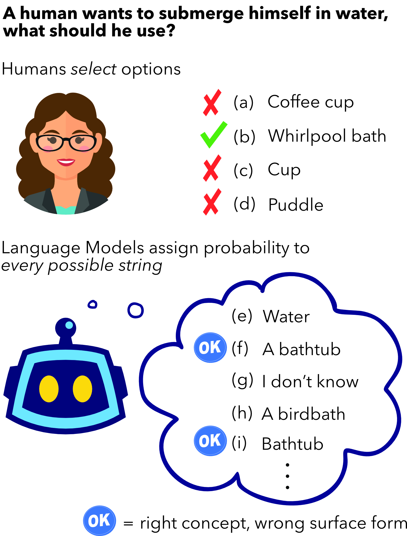
Figure 1: While humans select from given options, language models implicitly assign probability to every possible string. This creates surface form competition between different strings that represent the same concept. Example from CommonsenseQA Talmor et al. (2019).

We introduce Domain Conditional Pointwise Mutual Information, an alternative scoring function that directly compensates for surface form competition by simply reweighing each option according to its a priori likelihood within the context of a specific task. It achieves consistent gains in zero-shot performance over both calibrated Zhao et al. (2021) and uncalibrated scoring functions on all GPT-2 and GPT-3 models on a variety of multiple choice datasets.

1 Introduction

Despite the impressive results large pretrained language models have achieved in zero-shot settings Brown et al. (2020); Radford et al. (2019), we argue that current work underestimates the zero-shot capabilities of these models on classification tasks. This is in large part due to surface form competition—a property of generative models that causes probability to be rationed between different valid strings, even ones that differ trivially, e.g., by capitalization alone. Such competition can be largely removed by scoring choices according to Domain Conditional Pointwise Mutual Information ($\textrm{PMI}_{\textrm{DC}}$), which reweighs scores by how much more likely a hypothesis (answer) becomes given a premise (question) within the specific task domain.

Specifically, consider the example question (shown in Figure 1): “A human wants to submerge himself in water, what should he use?” with multiple choice options “Coffee cup”, “Whirlpool bath”, “Cup”, and “Puddle.” From the given options, “Whirlpool bath” is the only one that makes sense. Yet, other answers are valid and easier for a language model to generate, e.g., “Bathtub” and “A bathtub.” Since all surface forms compete for finite probability mass, allocating significant probability mass to “Bathtub” decreases the amount of probability mass assigned to “Whirlpool bath.” While the total probability of generating some correct answer may be high (i.e., across all valid surface forms), only one of these is a listed option. This is particularly problematic here, because “Whirlpool bath” will be much lower probability than “Bathtub,” due to its rarity. More generally, methods that do not account for surface form competition will favor answers with fewer lexical paraphrases.

$\textrm{PMI}_{\textrm{DC}}$ factors out the probability of a specific surface form, by instead computing how much more probable a hypothesis is when conditioned on a premise. We use a domain premise string to estimate the unconditional probability of a hypothesis in a given domain. On CommonsenseQA, for example, we compute the probability of each answer option immediately following the string “? the answer is:”, and then divide the conditional probability by this estimate to calculate $\textrm{PMI}_{\textrm{DC}}$. This scaling factor reweighs answer scores according to the surface form competition that is inherent to the domain or task, e.g. completions of the domain premise that are just inherently unlikely will be upweighted more. This allows us to directly measure how much an answer tells us about the question and vice versa (mutual information is symmetric, see §3). Valid hypotheses no longer need to compete with each other: both “Whirlpool bath” and “Bathtub ” will be considered reasonable answers to the question, and so both will attain a high score.

Extensive experiments show that $\textrm{PMI}_{\textrm{DC}}$ consistently outperforms raw, normalized, and calibrated probability scoring methods on zero-shot multiple choice for more than a dozen datasets and it does so for every model in the GPT-2 and GPT-3 families (§4); this holds true across different possible prompts and in preliminary few-shot experiments as well. To better explain these gains, we use the distinct structure of the COPA dataset Roemmele et al. (2011) to remove surface form competition entirely, showing that all methods perform well in this idealized setting (§5). Additionally, we analyze the only three datasets where $\textrm{PMI}_{\textrm{DC}}$ does worse than other methods and put forward a hypothesis for why normalizing log probabilities works better than raw probabilities (§6). We conclude with a discussion of how generative models should be used for selection tasks (§7).

2 Background and Related Work

Zero-shot vs. Few-Shot

Zero-shot inference has long been of interest in NLP, Computer Vision, and ML in general Socher et al. (2013); Guadarrama et al. (2013); Romera-Paredes and Torr (2015). However, Radford et al. (2019) popularized the notion that language models have many zero-shot capabilities that can be discovered simply by prompting the model, e.g., placing “TL;DR” (internet slang for Too Long; Didn’t Read) at the end of a passage causes the model to generate a summary. Efficiently constructing the right prompt for a given task is difficult and has become an active area of research Reynolds and McDonell (2021); Lu et al. (2021); Shin et al. (2020); Jiang et al. (2020a, b).

Brown et al. (2020) demonstrated that few-shot learning without fine-tuning is possible with very large language models. Contemporary work has shown it is possible to get smaller models to exhibit few-shot learning behavior using fine-tuning Hambardzumyan et al. (2021); Gao et al. (2020); Schick and Schütze (2020a, b, c); Shin et al. (2020), an intermediate learning phase Ye et al. (2021), or calibration Zhao et al. (2021), though most assume access to a validation set Perez et al. (2021). Recent work suggests it may be possible to finetune language models in order to improve their zero-shot and few-shot capabilities on a large swathe of tasks Wei et al. (2021); Zhong et al. (2021).

Surface Form Competition

When applying generative models to multiple choice problems, simply choosing the highest probability answer becomes problematic due to different valid surface forms competing for probability. Indeed, recent work in question answering has demonstrated the importance of considering all multiple choice options together Khashabi et al. (2020), rather than independently assigning each answer a score and simply choosing the highest. This is a difficult strategy to adapt to left-to-right generative language models, which implicitly choose between all possible strings. Using unsupervised language models pretrained on relatively expansive corpora exacerbates surface form competition because such language models generate a much wider distribution than a given question answering dataset contains.

“What is the most populous nation in North America?” Posed with this question, a language model such as GPT-3 can generate a correct response such as “USA”, ”United States”, or “United States of America” with high probability. While correct strings like this all contribute to the probability of a correct generation, they may have vastly different probabilities: a common string “United States” will be much more likely than rarer forms like “U.S. of A.”. In generative scenarios, as long as most of the probability mass goes to valid strings the generation is likely to be valid. This is not the case for multiple choice problems. Given two options, e.g., “USA” and “Canada”, GPT-3 will choose the correct answer by probability. However, if we substitute out “USA” for “U.S. of A.”, GPT-3 will assign higher probability to “Canada”, a less likely answer conceptually, but a much more likely surface form. Beyond this, incorrect generic answers such as “I don’t know” are often assigned high probability, relegating the desired answers to the tail of the distribution where softmax is poorly calibrated Holtzman et al. (2020).

PMI

Work in dialogue has used PMI to promote diversity Zhou et al. (2019); Yao et al. (2017); Li et al. (2016); Mou et al. (2016); Tang et al. (2019). Recently, Brown et al. (2020) used a scoring function resembling $\textrm{PMI}_{\textrm{DC}}$ for zero-shot question answering, though they only use the string “A:” as a prompt for the unconditional probability estimate, whereas we use a task-specific domain premise (see §3 for details). Furthermore, Brown et al. (2020) only report this scoring method on three datasets (ARC, OpenBookQA, and RACE, included here) out of the more than 20 tested and do not compare scores with their standard method, averaging log-likelihoods (Avg in this work). In contrast, we report a comprehensive comparison on GPT-3 and GPT-2, as well as shedding light on the underlying issue of surface form competition in §5.

Contextual Calibration

Recently, Zhao et al. (2021) describe a new method for calibrating the probabilities of an LM using a learned affine transformation. Though geared towards few-shot learning, the authors devise a clever means of using “content free inputs” for zero-shot learning. Zhao et al. (2021) calibrate for three forms of bias: (1) majority label bias, (2) recency bias, and (3) common token bias. $\textrm{PMI}_{\textrm{DC}}$ directly compensates for common token bias by dividing by the domain conditional probability of each answer, and performs superior to contextual calibration (CC) in the majority of cases.

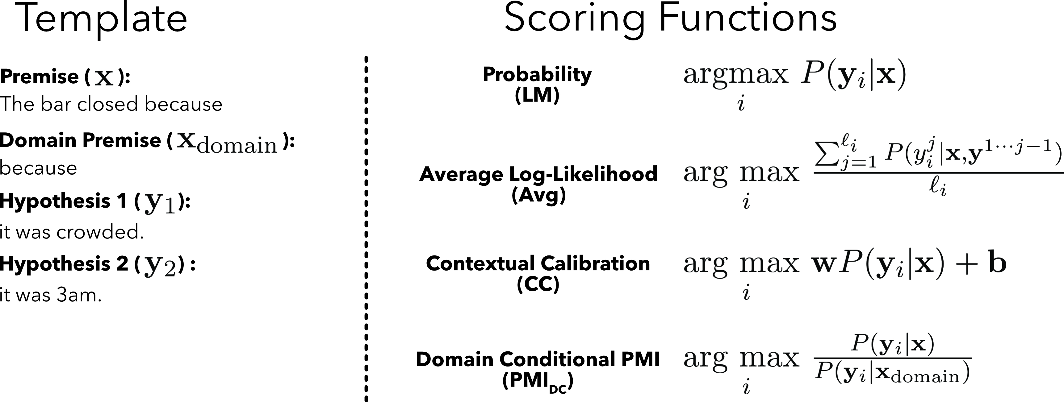
Figure 2: An example from COPA Roemmele et al. (2011) with the template we use as well as the scoring functions we test. LM returns the highest probability option, while Avg length-normalizes log-likelihoods and chooses the highest option. $\textrm{PMI}_{\textrm{DC}}$ is a measurement of the mutual information between hypothesis and premise, intuitively how much $\mathbf{x}$ explains $\mathbf{y}_{i}$ and vice versa. CC is an affine transform of LM, where $\mathbf{w}$ and $\mathbf{b}$ are averaged over solutions that cause “content free inputs” to yield uniform scores over a given label set, see Zhao et al. (2021).

Prompt Sensitivity

Recent work highlights LM sensitivity to inputs, and proposes to consider paraphrases of the prompt to overcome this Davison et al. (2019); Jiang et al. (2020b), as well as noting that certain trigger tokens Shin et al. (2020) can strongly effect the output of such models. In this work, we focus on the surface form of possible outputs, but do also analyze robustness to different prompts in §4.4.

Interpreting Language Models

Language models tend to model selectional preferences and thematic fit Pantel et al. (2007); Erk et al. (2010) rather than semantic plausibility Wang et al. (2018). Probability, possibility and plausibility are distinct Van der Helm (2006), but reporting bias Gordon and Van Durme (2013) means that language models only model what people are likely to write (on websites that are easily crawled). $\textrm{PMI}_{\textrm{DC}}$ aims to adjust for these challenges to better measure the underlying agreement between language models and human judgements, but of course is still subject to the limits and biases of the language model used.

3 Zero-shot Scoring Strategies

This paper does not define any new modeling or finetuning methods. Rather, we propose the broad use of $\textrm{PMI}_{\textrm{DC}}$ scoring for any given model and prompt. $\textrm{PMI}_{\textrm{DC}}$ compensates for the fact that different correct answers compete for probability, even though only one will be listed as the correct multiple choice option.

We begin by describing the two most common methods currently in use.

3.1 Standard Methods

Our first baseline is simply selecting the highest-probability option, e.g., baselines in Zhao et al. (2021) and Jiang et al. (2020b), which we refer to as LM. Given a prompt $\mathbf{x}$ (e.g. “The bar closed”) and a set of possible answers $\mathbf{y}_{1},\cdots,\mathbf{y}_{n}$ (e.g. “it was crowded.”, “it was 3 AM.”), LM is defined:

$$\operatorname*{arg\,max}_{i}P(\mathbf{y}_{i}|\mathbf{x}).$$ (1)

However, using length normalized log-likelihoods Brown et al. (2020) has become standard due to its superior performance, and is also commonly used in generation Mao et al. (2019); Oluwatobi and Mueller (2020). For causal language models, e.g., GPT-2 and GPT-3, Equation 1 can be decomposed:

$$P(\mathbf{y}_{i}|\mathbf{x})=\prod_{j=1}^{\ell_{i}}P(y_{i}^{j}|\mathbf{x},y_{i}^{1},\cdots,y_{i}^{j-1})$$

where $y_{i}^{j}$ is the $j$th token of $\mathbf{y}_{i}$ and $\ell_{i}$ is the number of tokens in $\mathbf{y}_{i}$. The Avg strategy can thus be defined as:

$$\operatorname*{arg\,max}_{i}\frac{\sum^{\ell_{i}}_{j=1}\log P(y_{i}^{j}|\mathbf{x},\mathbf{y}^{1\cdots j-1})}{\ell_{i}}.\\$$

3.2 Domain Conditional PMI

Our core claim is that direct probability is not an adequate zero-shot scoring function due to surface form competition. A natural solution is to factor out the probability of specific surface forms, which is what Pointwise Mutual Information (PMI) does:

$$\textrm{PMI}(\mathbf{x},\mathbf{y})=\log\frac{P(\mathbf{y}|\mathbf{x})}{P(\mathbf{y})}=\log\frac{P(\mathbf{x}|\mathbf{y})}{P(\mathbf{x})}.$$ (2)

In effect, this is how much more likely the hypothesis (“it was 3 AM.”) becomes given the premise (“The bar closed because”), see Figure 2 for the full example. In a multiple-choice setting—where the premise $\mathbf{x}$ does not change across hypotheses—this is proportional to $P(\mathbf{x}|\mathbf{y})$, i.e. the probability of the premise given the hypothesis. We call this scoring-by-premise and it is the reverse of LM, $P(\mathbf{y}|\mathbf{x})$. We use scoring-by-premise to show the presence of surface form competition in §5.

While Equation 2 estimates how related premise $\mathbf{x}$ is to hypothesis $\mathbf{y}$ in general, we found that estimates of $P(\mathbf{y})$ vary wildly. GPT-2 and GPT-3 are not trained to produce unconditional estimates of document excerpts, an issue which is exacerbated by the fact that many possible answers are extremely rare in a large scrape of public web pages. This causes the unconditional probability of such answers to be poorly calibrated for the purposes of a given task.

We are specifically trying to measure $P(\mathbf{y})$ in a given domain, e.g., for the “because” relation in our running example, shown in Figures 2 & 3. To quantify this, we propose Domain Conditional PMI:

$$\exp\textrm{PMI}_{\textrm{DC}}(\mathbf{x},\mathbf{y},\textrm{domain}) =\frac{P(\mathbf{y}|\mathbf{x},\textrm{domain})}{P(\mathbf{y}|\textrm{domain})}$$

$$=\frac{P(\mathbf{y}|\mathbf{x},\textrm{domain})}{P(\mathbf{y}|\mathbf{x}_{\textrm{domain}})}$$

or how much $\mathbf{x}$ tells us about $\mathbf{y}$ within a domain.

Typically, $P(\mathbf{y}|\mathbf{x},\textrm{domain})=P(\mathbf{y}|\mathbf{x})$ because the premise $\mathbf{x}$ typically implies the domain, e.g., “The bar closed because” sets the model up to predict an independent clause that is the cause of some event, without further representation of the domain. In order to estimate $P(\mathbf{y}|\textrm{domain})$—the probability of seeing hypothesis $\mathbf{y}$ in a given domain—we use a short domain-relevant string $\mathbf{x}_{\textrm{domain}}$, which we call a “domain premise”, usually just the ending of the conditional premise $\mathbf{x}$. For example, to predict a causal relation like in Figure 2 we use $\mathbf{x}_{\textrm{domain}}=\textrm{``because''}$ and thus divide by $P(\mathbf{y}|\textrm{because})$–how likely $y$ is to be a “cause” . For examples of each template see Appendix B.

3.3 Non-standard Baselines

Unconditional

We also compare to the unconditional (in-domain) estimate as a scoring function:

$$\operatorname*{arg\,max}_{i}P(\mathbf{y}_{i}|\mathbf{x}_{\textrm{domain}}).$$

We refer to this as Unc. It ignores the premise completely, only using a domain premise $\mathbf{x}_{\textrm{domain}}$ (e.g., using $P(\mathbf{y}|\textrm{because})$ as the score). Yet, it is sometimes competitive, for instance on BoolQ Clark et al. (2019). Unc is a sanity check on whether zero-shot inference is actually using the information in the question to good effect.

Contextual Calibration

Finally, we compare to the reported zero-shot numbers of Zhao et al. (2021). Contextual Calibration adjusts LM with an affine transform to make a closed set of answers equally likely in the absence of evidence. Contextual Calibration thus requires computing matrices $\mathbf{w}$ and $\mathbf{b}$ for a number of “content free inputs” and then averaging these weights, see Zhao et al. (2021) for details. In contrast, $\textrm{PMI}_{\textrm{DC}}$ requires nothing but a human-written template (as all zero-shot methods do, including Contextual Calibration), can be computed as the difference of two log probabilities, and is naturally applicable to datasets where the set of valid answers varies between questions.

4 Multiple Choice Experiments

4.1 Setup

We use GPT-2 via the HuggingFace Transformers library Wolf et al. (2020) and GPT-3 via OpenAI’s beta API. We do not finetune any models, nor do we alter their output. See Appendix B for examples from each dataset in our templated format.

4.2 Datasets

We report results on 16 splits of 13 datasets, and briefly describe each dataset here.

Continuation

These datasets require the model to select a continuation to previous text, making them a natural way to test language models. Choice of Plausible Alternatives (COPA) Roemmele et al. (2011) asks for cause and effect relationships, as shown in Figure 2. StoryCloze (SC) Mostafazadeh et al. (2017) gives the model a choice between two alternative endings to 5 sentence stories. Finally, HellaSwag (HS) Zellers et al. (2019) uses GPT-2 to generate, BERT to filter, and crowd workers to verify possible continuations to a passage. Following previous work Brown et al. (2020) we report development set numbers for COPA and HS.

Question Answering

RACE-M & -H (R-M & R-H) Lai et al. (2017) are both drawn from English exams given in China, the former being given to Middle Schoolers and the latter to High Schoolers. Similarly, ARC Easy & Challenge (ARC-E & ARC-C) Clark et al. (2018) are standardized tests described as “natural, grade-school science questions,” with the “Easy” split found to be solvable by either a retrieval or word co-occurrence system, and the rest of the questions put in the “Challenge” split. Open Book Question Answering (OBQA) Mihaylov et al. (2018) is similar to both of these, but was derived using (and intended to be tested with) a knowledge source (or “book”) available; we do not make use of the given knowledge source, following Brown et al. (2020). Finally, CommonsenseQA (CQA) Talmor et al. (2019) leverages ConceptNet Speer et al. (2017) to encourage crowd workers to write questions with challenging distractors. We report development set numbers on CQA because their test set is not public.

Multiple Choice Accuracy on GPT-3

Params.	2.7B					6.7B				13B				175B
	Unc	LM	Avg	$\textrm{PMI}_{\textrm{DC}}$	CC	Unc	LM	Avg	$\textrm{PMI}_{\textrm{DC}}$	Unc	LM	Avg	$\textrm{PMI}_{\textrm{DC}}$	Unc	LM	Avg	$\textrm{PMI}_{\textrm{DC}}$	CC
COPA	54.8	68.4	68.4	74.4	-	56.4	75.8	73.6	77.0	56.6	79.2	77.8	84.2	56.0	85.2	82.8	89.2	-
SC	50.9	66.0	68.3	73.1	-	51.4	70.2	73.3	76.8	52.0	74.1	77.8	79.9	51.9	79.3	83.1	84.0	-
HS	31.1	34.5	41.4	34.2	-	34.7	40.8	53.5	40.0	38.8	48.8	66.2	45.8	43.5	57.6	77.2	53.5	-
R-M	22.4	37.8	42.4	42.6	-	21.2	43.3	45.9	48.5	22.9	49.6	50.6	51.3	22.5	55.7	56.4	55.7	-
R-H	21.4	30.3	32.7	36.0	-	22.0	34.8	36.8	39.8	22.9	38.2	39.2	42.1	22.2	42.4	43.3	43.7	-
ARC-E	31.6	50.4	44.7	44.7	-	33.5	58.2	52.3	51.5	33.8	66.2	59.7	57.7	36.2	73.5	67.0	63.3	-
ARC-C	21.1	21.6	25.5	30.5	-	21.8	26.8	29.8	33.0	22.3	32.1	34.3	38.5	22.6	40.2	43.2	45.5	-
OBQA	10.0	17.2	27.2	42.8	-	11.4	22.4	35.4	48.0	10.4	28.2	41.2	50.4	10.6	33.2	43.8	58.0	-
CQA	15.9	33.2	36.0	44.7	-	17.4	40.0	42.9	50.3	16.4	48.8	47.9	58.5	16.3	61.0	57.4	66.7	-
BQ	62.2	58.5	58.5	53.5	-	37.8	61.0	61.0	61.0	62.2	61.1	61.1	60.3	37.8	62.5	62.5	64.0	-
RTE	47.3	48.7	48.7	51.6	49.5	52.7	55.2	55.2	48.7	52.7	52.7	52.7	54.9	47.3	56.0	56.0	64.3	57.8
CB	08.9	51.8	51.8	57.1	50.0	08.9	33.9	33.9	39.3	08.9	51.8	51.8	50.0	08.9	48.2	48.2	50.0	48.2
SST-2	49.9	53.7	53.76	72.3	71.4	49.9	54.5	54.5	80.0	49.9	69.0	69.0	81.0	49.9	63.6	63.6	71.4	75.8
SST-5	18.1	20.0	20.4	23.5	-	18.1	27.8	22.7	32.0	18.1	18.6	29.6	19.1	17.6	27.0	27.3	29.6	-
AGN	25.0	69.0	69.0	67.9	63.2	25.0	64.2	64.2	57.4	25.0	69.8	69.8	70.3	25.0	75.4	75.4	74.7	73.9
TREC	13.0	29.4	19.2	57.2	38.8	22.6	30.2	22.8	61.6	22.6	34.0	21.4	32.4	22.6	47.2	25.4	58.4	57.4

Table 1: Comparison of scoring algorithms when using GPT-3 for zero-shot inference on multiple choice questions.

Percent of Ties or Wins by Method

Method	Unc	LM	Avg	$\textrm{PMI}_{\textrm{DC}}$	CC
125M	12.50	6.25	12.50	68.75	-
350M	6.25	18.75	12.50	68.75	-
760M	6.25	6.25	12.50	75.00	-
1.6B	6.25	12.50	12.50	80.00	20.00
2.7B	6.25	6.25	6.25	86.66	0.00
6.7B	6.25	25.00	25.00	75.00	-
13B	6.25	18.75	18.75	68.75	-
175B	6.25	12.50	18.75	62.50	6.25

Table 2: Percentage of datasets that a given method produced the best score or was tied with other methods, aggregated over each model size. The first four rows use GPT-2 (full data available in the Appendix), while the final four rows use GPT-3 and summarize data from Table 1. Since ties are included, rows sometimes sum to more than 100. CC is only measured on the 5 datasets we use where Zhao et al. (2021) also report accuracies.

Open Set vs. Closed Set Datasets

The above datasets are all “open set” in that multiple choice answers may be any string. Below we describe “closed set” datasets with a fixed set of answers.

Boolean Question Answering

BoolQ (BQ) Clark et al. (2019) poses yes/no (i.e. Boolean) questions based on a multi-sentence passage.

Entailment

Entailment datasets focus on the question of whether a hypothesis sentence B is entailed by a premise sentence A. Recognizing Textual Entailment (RTE) Dagan et al. (2005) requires predicting an “entailment” or “contradiction” label while Commitment Bank (CB) De Marneffe et al. (2019) adds a “neutral” label. Following previous work Brown et al. (2020) we report development set numbers for both RTE and CB.

Text Classification

We consider three more complex classification datasets: SST-2 & -5 Socher et al. (2013) for various granularities of sentiment classification, AG’s News Zhang et al. (2015) (AGN) for topic classification, and TREC Li and Roth (2002) for question classification.

4.3 Results

We report zero-shot results for GPT-3 in Table 1, with GPT-2 results available in Appendix A. A summarized view is shown in Table 2, which aggregates the percentage of splits where a given method achieves the best score or ties for first-place. In this summarized view it is clear that $\textrm{PMI}_{\textrm{DC}}$ consistently outperforms other scoring methods when assessed over a variety of datasets. The smallest margin (in number of datasets won or tied) between $\textrm{PMI}_{\textrm{DC}}$ and the best competing method is on GPT-3 175B with Avg, but that margin is over 40 percentage points. This does not imply that $\textrm{PMI}_{\textrm{DC}}$ is always better or that it will be better by a large margin, though it often is. It does suggest that $\textrm{PMI}_{\textrm{DC}}$ is a significantly better bet on a new dataset.

Prompt Robustness on SST-2

Method	Unc	LM	$\textrm{PMI}_{\textrm{DC}}$
125M	$\textrm{49.9}_{\textrm{~{}0}}$	$\textrm{56.8}_{\textrm{~{}7.3}}$	$\textrm{{58.8}}_{\textrm{~{}7.6}}$
350M	$\textrm{49.9}_{\textrm{~{}0}}$	$\textrm{58.0}_{\textrm{~{}11.3}}$	$\textrm{{60.3}}_{\textrm{~{}11.4}}$
760M	$\textrm{49.9}_{\textrm{~{}0}}$	$\textrm{57.0}_{\textrm{~{}9.2}}$	$\textrm{{67.7}}_{\textrm{~{}13.4}}$
1.6B	$\textrm{49.9}_{\textrm{~{}0}}$	$\textrm{57.3}_{\textrm{~{}8.2}}$	$\textrm{{69.8}}_{\textrm{~{}13.3}}$
2.7B	$\textrm{49.9}_{\textrm{~{}0}}$	$\textrm{56.1}_{\textrm{~{}9.0}}$	$\textrm{{66.2}}_{\textrm{~{}15.7}}$
6.7B	$\textrm{49.9}_{\textrm{~{}0}}$	$\textrm{59.5}_{\textrm{~{}10.7}}$	$\textrm{{67.9}}_{\textrm{~{}13.6}}$
13B	$\textrm{49.9}_{\textrm{~{}0}}$	$\textrm{63.0}_{\textrm{~{}14.9}}$	$\textrm{{71.7}}_{\textrm{~{}16.1}}$
175B	$\textrm{49.9}_{\textrm{~{}0}}$	$\textrm{72.5}_{\textrm{~{}15.7}}$	$\textrm{{74.8}}_{\textrm{~{}14.0}}$

Table 3: The mean and standard deviations over the 15 templates considered for SST-2 in Zhao et al. (2021). Avg is excluded, as it is equivalent to LM since all the given templates use single-token answers.

4-shot Inference Results

SST-2				CQA
Method	Unc	LM	$\textrm{PMI}_{\textrm{DC}}$	Unc	LM	Avg	$\textrm{PMI}_{\textrm{DC}}$
125M	$\textrm{49.9}_{\textrm{~{}0}}$	$\textrm{63.6}_{\textrm{~{}7.4}}$	$\textrm{{71.7}}_{\textrm{~{}5.1}}$	$\textrm{15.5}_{\textrm{~{}0}}$	$\textrm{29.9}_{\textrm{~{}1.6}}$	$\textrm{32.7}_{\textrm{~{}1.4}}$	$\textrm{{38.3}}_{\textrm{~{}1.7}}$
350M	$\textrm{49.9}_{\textrm{~{}0}}$	$\textrm{76.3}_{\textrm{~{}13.8}}$	$\textrm{{76.4}}_{\textrm{~{}8.1}}$	$\textrm{16.5}_{\textrm{~{}0}}$	$\textrm{37.6}_{\textrm{~{}2.3}}$	$\textrm{40.4}_{\textrm{~{}2.3}}$	$\textrm{{45.7}}_{\textrm{~{}2.4}}$
760M	$\textrm{49.9}_{\textrm{~{}0}}$	$\textrm{85.9}_{\textrm{~{}7.2}}$	$\textrm{{87.1}}_{\textrm{~{}3.0}}$	$\textrm{16.1}_{\textrm{~{}0}}$	$\textrm{41.5}_{\textrm{~{}2.6}}$	$\textrm{42.4}_{\textrm{~{}2.5}}$	$\textrm{{47.0}}_{\textrm{~{}1.5}}$
1.6B	$\textrm{49.9}_{\textrm{~{}0}}$	$\textrm{85.4}_{\textrm{~{}1.7}}$	$\textrm{{89.4}}_{\textrm{~{}4.0}}$	$\textrm{16.0}_{\textrm{~{}0}}$	$\textrm{46.2}_{\textrm{~{}1.5}}$	$\textrm{47.7}_{\textrm{~{}1.9}}$	$\textrm{{52.3}}_{\textrm{~{}2.1}}$
2.7B	$\textrm{49.9}_{\textrm{~{}0}}$	$\textrm{{88.1}}_{\textrm{~{}4.9}}$	$\textrm{87.7}_{\textrm{~{}5.5}}$	$\textrm{16.6}_{\textrm{~{}0}}$	$\textrm{43.0}_{\textrm{~{}1.7}}$	$\textrm{45.6}_{\textrm{~{}1.9}}$	$\textrm{{50.4}}_{\textrm{~{}1.1}}$
6.7B	$\textrm{49.9}_{\textrm{~{}0}}$	$\textrm{{92.9}}_{\textrm{~{}2.1}}$	$\textrm{79.8}_{\textrm{~{}6.9}}$	$\textrm{16.9}_{\textrm{~{}0}}$	$\textrm{52.3}_{\textrm{~{}1.4}}$	$\textrm{53.4}_{\textrm{~{}1.0}}$	$\textrm{{56.5}}_{\textrm{~{}1.6}}$
13B	$\textrm{49.9}_{\textrm{~{}0}}$	$\textrm{85.4}_{\textrm{~{}9.0}}$	$\textrm{{86.9}}_{\textrm{~{}7.5}}$	$\textrm{16.7}_{\textrm{~{}0}}$	$\textrm{58.4}_{\textrm{~{}2.0}}$	$\textrm{59.3}_{\textrm{~{}1.5}}$	$\textrm{{63.4}}_{\textrm{~{}1.4}}$
175B	$\textrm{49.9}_{\textrm{~{}0}}$	$\textrm{89.9}_{\textrm{~{}5.5}}$	$\textrm{{95.5}}_{\textrm{~{}0.7}}$	$\textrm{16.5}_{\textrm{~{}0}}$	$\textrm{69.1}_{\textrm{~{}1.9}}$	$\textrm{69.4}_{\textrm{~{}0.8}}$	$\textrm{{72.0}}_{\textrm{~{}0.9}}$

Table 4: The mean and standard deviation for 5 randomly sampled sets of 4 examples used for few-shot inference. We include a closed answer dataset (SST-2) and an open answer dataset (CQA). For SST-2 Avg is equivalent to LM due to using single-token answers.

4.4 Robustness

To verify that these trends hold across different prompts, we report the mean and standard deviation over the fifteen different prompts considered in Zhao et al. (2021) for SST-2. Table 3 shows, $\textrm{PMI}_{\textrm{DC}}$ always maintains the highest mean, often by a hefty margin. Scores are lower than in Table 1 because many of the prompts used are optimized for few-shot rather than zero-shot scoring.

4.5 Few-shot

While our focus in this paper is on zero-shot scoring, $\textrm{PMI}_{\textrm{DC}}$ is just as applicable to few-shot scenarios. In Table 4 we report 4-shot results on one closed set dataset (SST-2) and one open set dataset (CQA). We show the mean of 5 randomly sampled sets of 4 examples that are used to prime the model for the task, along with standard deviations. The overall trend on both datasets clearly favors $\textrm{PMI}_{\textrm{DC}}$, though LM is superior for two models on SST-2.

5 Removing Surface Form Competition

What if we used the probability of the premise given the hypothesis, $P(\mathbf{x}|\mathbf{y}_{i})$, instead? While we are still measuring the probability of a surface form (e.g. “the bar closed.”), it is the same surface form across different options (“It was crowded so”, “It was 3 AM so”), eliminating the surface form competition. $\mathbf{y}_{i}$ and $\mathbf{y}_{i}^{\prime}$ can now both attain high scores if they are both correct answers, by causing $\mathbf{x}$ to be likely. We call this scoring-by-premise.

Causal language models like GPT-3 cannot measure this directly, because they are only capable of conditioning on past tokens to predict future tokens. We exploit the structure of the COPA dataset to create “COPA Flipped” via a simple transformation, shown in Figure 3. COPA consists of cause and effect pairs (CAUSE so EFFECT, and EFFECT because CAUSE). In the original dataset, whatever comes second (either CAUSE or EFFECT) has two options that a model must choose between. These can be reversed by switching CAUSE and EFFECT, then substituting the natural inverse relation (“because”$\xrightarrow{}$“so” and “so”$\xrightarrow{}$“because” ).

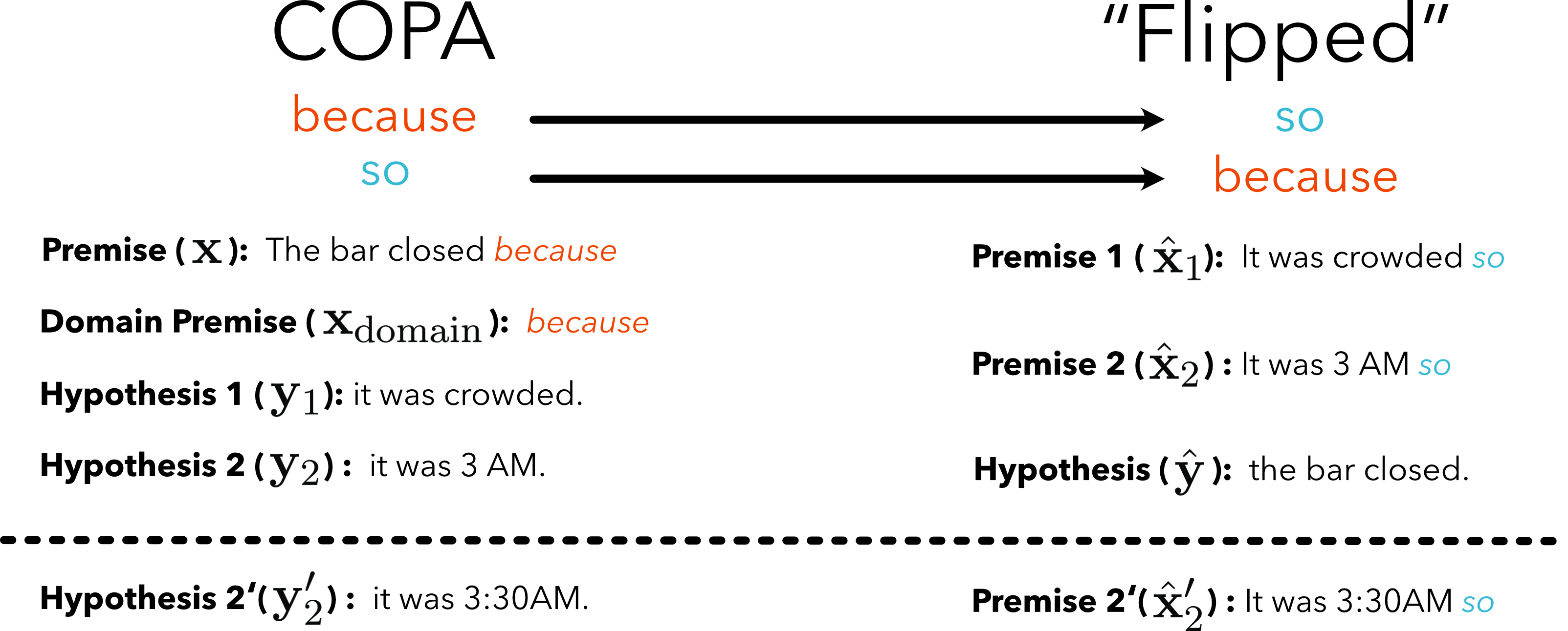
Figure 3: In §5 we experiment with with flipping the premise and hypothesis so that the highest probability premise is chosen as the answer, i.e. scoring-by-premise. The transformation above the dashed line shows the experimental setup used in §5.1, while the extra distractor below the dashed line is used for illustrative purposes in §5.2.

5.1 Results

Table 5 shows scores on COPA and COPA Flipped side-by-side. On COPA Flipped everything except Unc produces the exact same result. This is because flipping the hypothesis and premise means that it’s the context that changes and not the continuation. LM, Avg, and $\textrm{PMI}_{\textrm{DC}}$ only differ from each other over different continuations, not over different contexts for the same continuation.

Removing Surface Form Competition

COPA					COPA Flipped
Method	Unc	LM	Avg	$\textrm{PMI}_{\textrm{DC}}$	Unc	LM	Avg	$\textrm{PMI}_{\textrm{DC}}$
125M	56.4	61.0	63.2	62.8	50.0	63.2	63.2	63.2
350M	55.8	67.0	66.0	70.0	50.0	66.4	66.4	66.4
760M	55.6	69.8	67.6	69.4	50.0	70.8	70.8	70.8
1.6B	56.0	69.0	68.4	71.6	50.0	73.0	73.0	73.0
2.7B	54.8	68.4	68.4	74.4	50.0	68.4	68.4	68.4
6.7B	56.4	75.8	73.6	77.0	50.0	76.8	76.8	76.8
13B	56.6	79.2	77.8	84.2	50.0	79.0	79.0	79.0
175B	56.0	85.2	82.8	89.2	50.0	83.6	83.6	83.6

Table 5: LM does better on COPA Flipped than COPA because surface form competition is removed when scoring-by-premise, see §5. Methods that don’t directly adjust for competing surface forms (LM and Avg ) have the same score as $\textrm{PMI}_{\textrm{DC}}$ on COPA Flipped.

On COPA Flipped all methods generally perform similarly to $\textrm{PMI}_{\textrm{DC}}$ on the unflipped version. This is because surface form competition has been eradicated: we are measuring how well different prefixes condition a model to predict a fixed continuation rather than which continuation is highest probability. Unlike LM, where different answers compete for probability, in COPA Flipped it only matters how likely each answer can make the question. This is not subject to surface form competition because there is only one string being so scored, so it is not competing with any other strings for probability mass.

Not all datasets are so easily flippable, so manually flipping individual questions to remove surface form competition is not a generally applicable strategy. Luckily, $\textrm{PMI}_{\textrm{DC}}$ is symmetric:

$$\operatorname*{arg\,max}_{i}\frac{P(\mathbf{y}_{i}|\mathbf{x},\textrm{domain})}{P(\mathbf{y}_{i}|\textrm{domain})}$$

$$= \operatorname*{arg\,max}_{i}\frac{P(\mathbf{x}|\mathbf{y}_{i},\textrm{domain})}{P(\mathbf{x}|\textrm{domain})}$$

$$= \operatorname*{arg\,max}_{i}P(\mathbf{x}|\mathbf{y}_{i},\textrm{domain})$$

In theory, the answer selected by $\textrm{PMI}_{\textrm{DC}}$ should be the same between COPA and COPA Flipped as PMI is symmetric, though we expect some differences due to “so” and “because” not being perfect inverses and shuffled references. Thus, $\textrm{PMI}_{\textrm{DC}}$ does better on COPA than COPA Flipped, likely due to more natural phrasing in the original dataset.

These results suggest that surface form competition is the primary cause of the depressed performance of LM and Avg in comparison to $\textrm{PMI}_{\textrm{DC}}$.

5.2 In-depth Example

Scoring-by-Premise Improves LM

Figure 3 shows an example of transforming one question from COPA to COPA Flipped. In the example depicted, when we use GPT-3 to calculate $P$, we get:

$$P(\mathbf{y}_{1}|\mathbf{x})>P(\mathbf{y}_{2}|\mathbf{x})$$

which is wrong, since bars usually close at fixed, late-night closing times, rather than because of being overcrowded. However we also find that

$$P(\hat{\mathbf{y}}|\hat{\mathbf{x}}_{2}) >P(\hat{\mathbf{y}}|\hat{\mathbf{x}}_{1})$$

$$\frac{P(\mathbf{y}_{2}|\mathbf{x})}{P(\mathbf{y}_{2}|\mathbf{x}_{\textrm{domain}})} >\frac{P(\mathbf{y}_{1}|\mathbf{x})}{P(\mathbf{y}_{1}|\mathbf{x}_{\textrm{domain}})}$$

indicating that scoring-by-premise causes the right answer to be selected and that $\textrm{PMI}_{\textrm{DC}}$ successfully simulates scoring by premise in this example.

Stability Over Valid Answers

To see how scoring-by-premise allows multiple correct options to achieve high scores, consider the slightly perturbed $\mathbf{y}^{\prime}_{2}$ and $\hat{\mathbf{x}}_{2}^{\prime}$ in Figure 3. The inequalities shown above still hold when substituting                 $\mathbf{y}_{2}\rightarrow\mathbf{y}_{2}^{\prime}$ and $\hat{\mathbf{x}}_{2}\rightarrow\hat{\mathbf{x}}_{2}^{\prime}$:

$$P(\mathbf{y}_{1}|\mathbf{x}) >P(\mathbf{y}_{2}^{\prime}|\mathbf{x})$$

$$P(\hat{\mathbf{y}}|\hat{\mathbf{x}}_{2}^{\prime}) >P(\hat{\mathbf{y}}|\hat{\mathbf{x}}_{1})$$

$$\frac{P(\mathbf{y}_{2}^{\prime}|\mathbf{x})}{P(\mathbf{y}_{2}^{\prime}|\mathbf{x}_{\textrm{domain}})} >\frac{P(\mathbf{y}_{1}|\mathbf{x})}{P(\mathbf{y}_{1}|\mathbf{x}_{\textrm{domain}})}$$

with the key difference that the conditional probability of $\mathbf{y}^{\prime}_{2}$ is much lower:

$$\log{P(\mathbf{y}_{2}|\mathbf{x})} \approx-16$$

$$\log{P(\mathbf{y}_{2}^{\prime}|\mathbf{x})} \approx-20$$

This is undesirable, as both $\mathbf{y}_{2}$ and $\mathbf{y}^{\prime}_{2}$ are correct answers with similar meanings. Yet, when scoring-by-premise the conditional probability of $\hat{\mathbf{y}}$ is stable when substituting $\hat{\mathbf{x}}_{2}\rightarrow\hat{\mathbf{x}}_{2}^{\prime}$:

$$\log{P(\hat{\mathbf{y}}|\hat{\mathbf{x}}_{2})} \approx-12$$

$$\log{P(\hat{\mathbf{y}}|\hat{\mathbf{x}}_{2}^{\prime})} \approx-12$$

This suggests that eliminating surface form competition allows different correct answers to score well, as they are no longer competing for probability mass. Specifically, “it was 3 AM” and “it was 3:30AM” score wildly differently in COPA but nearly identically in COPA Flipped.

6 Analysis

Failure Cases

There are three datasets where $\textrm{PMI}_{\textrm{DC}}$ does not consistently outperform other methods: HellaSwag, ARC Easy, and BoolQ. Surprisingly, each is dominated by a different method.

HellaSwag is most amenable to Avg. On examination we find that HellaSwag is more focused on the internal coherence of the hypotheses, rather than external coherence, i.e. how much a premise and hypothesis match. This is likely due to HellaSwag being generated by GPT-2 Radford et al. (2019) and filtered with BERT, as it contains relatively on-topic but intrinsically strange hypotheses that humans can distinguish from natural data.

ARC Easy yields the highest scores to LM, i.e., selecting the highest probability option. Clark et al. (2018) note that ARC Easy questions can be solved by a retrieval or word co-occurrence baseline, while examples that were answered incorrectly by both were put into the Challenge split. This suggests a bias towards a priori likely phrases. Manual inspection reveals many stock answers, e.g., “[clouds are generated when] ocean water evaporates and then condenses in the air,” supporting our hypothesis.

Finally, BoolQ, a reading comprehension dataset in which all answers are either “yes” or “no”, is best solved by an unconditional baseline. This is because the dataset presents truly complex questions that require more reasoning than GPT-2 or 3 are capable of out of the box. Indeed, none of the methods reported do better than the majority baseline, except $\textrm{PMI}_{\textrm{DC}}$ with the largest GPT-3 model.

Why does length normalization work?

Past work offers little explanation for why Avg should be a successful strategy, other than the intuition that estimates are strongly length biased and require compensation. Length bias may be caused by the final softmax layer of current language models assigning too much probability mass to irrelevant options at each time-step, as noted in open-ended generation, character-level language modeling, and machine translation Holtzman et al. (2020); Al-Rfou et al. (2019); Peters et al. (2019).

Another (not mutually exclusive) argument is that length normalization may account for unconditional probability in a similar way to $\textrm{PMI}_{\textrm{DC}}$. Length normalization is often measured over Byte Pair Encoding (BPE) tokens Sennrich et al. (2016) and BPE tends to produce vocabularies where most tokens are equally frequent Wang et al. (2020). Recent evidence suggests that language is approximately uniformly information dense Levy (2018); Levy and Jaeger (2007); Jaeger (2006). As such, length in BPE tokens may correspond roughly to a unigram estimate of log-probability, supposing that BPE tokens have approximately uniform unigram frequency. The adjustment made by Avg is still somewhat different than $\textrm{PMI}_{\textrm{DC}}$, (division of log terms rather than subtraction) but could have a similar effect, if length and probability correlate.

7 Discussion

Language Models are density estimation functions that assign probability to every possible string, but there are often many strings that could represent a given idea equally well. Our key observation is that a generative model assigning probability to a string that represents a certain option isn’t equivalent to selecting the concept an option corresponds to. We expect surface form competition anywhere that generative models are used where more than one string could represent the same concept.

$\textrm{PMI}_{\textrm{DC}}$ aligns the predictions being made by the model more closely with the actual task posed by multiple choice questions: “choose the hypothesis that explains the premise” rather than “generate the exact surface form of the hypothesis”. From this perspective, $\textrm{PMI}_{\textrm{DC}}$ does not go far enough, because the model still cannot consider the given set of options altogether when selecting its choice. This matters when answers interact with each other, e.g., “all of the above”.

8 Conclusion

We conduct a large-scale comparison of standard and recent scoring functions for zero-shot inference across all GPT-2 and GPT-3 models. We show that $\textrm{PMI}_{\textrm{DC}}$ consistently outperforms previous scoring functions on a wide variety of multiple choice datasets. We also argue that compensating for surface form competition is the cause of this boost, by demonstrating that other methods work just as well as $\textrm{PMI}_{\textrm{DC}}$ when surface form competition is eliminated. In future work we would like to explore how surface form competition affects generation, as we hypothesize that it may be the cause of overly generic outputs under high model uncertainty.

Multiple Choice Accuracy on GPT-2

Params.	125M				350M				760M				1.6B
	Unc	LM	Avg	$\textrm{PMI}_{\textrm{DC}}$	Unc	LM	Avg	$\textrm{PMI}_{\textrm{DC}}$	Unc	LM	Avg	$\textrm{PMI}_{\textrm{DC}}$	Unc	LM	Avg	$\textrm{PMI}_{\textrm{DC}}$	CC
COPA	0.564	0.610	0.632	0.628	0.558	0.670	0.660	0.700	0.556	0.698	0.676	0.694	0.560	0.690	0.684	0.716	-
SC	0.495	0.600	0.615	0.670	0.489	0.630	0.667	0.716	0.503	0.661	0.688	0.734	0.512	0.676	0.715	0.763	-
HS	0.271	0.286	0.295	0.291	0.298	0.322	0.376	0.328	0.309	0.350	0.432	0.351	0.331	0.384	0.489	0.378	-
R-M	0.222	0.361	0.406	0.409	0.213	0.387	0.420	0.424	0.214	0.393	0.439	0.439	0.223	0.415	0.446	0.447	-
R-H	0.209	0.275	0.310	0.344	0.215	0.304	0.326	0.363	0.215	0.318	0.345	0.383	0.219	0.330	0.357	0.391	-
ARC-E	0.313	0.429	0.378	0.393	0.327	0.494	0.434	0.424	0.334	0.527	0.467	0.470	0.334	0.562	0.496	0.499	-
ARC-C	0.198	0.201	0.235	0.282	0.197	0.228	0.254	0.286	0.221	0.231	0.266	0.316	0.211	0.252	0.279	0.338	-
OBQA	0.11	0.164	0.272	0.324	0.108	0.186	0.302	0.386	0.108	0.194	0.296	0.432	0.114	0.224	0.348	0.460	-
CQA	0.170	0.255	0.307	0.364	0.165	0.309	0.352	0.418	0.170	0.333	0.368	0.445	0.171	0.386	0.385	0.478	-
BQ	0.622	0.588	0.588	0.511	0.622	0.608	0.608	0.497	0.622	0.580	0.580	0.467	0.622	0.563	0.563	0.495	-
RTE	0.527	0.516	0.516	0.498	0.473	0.531	0.531	0.549	0.473	0.531	0.531	0.542	0.473	0.477	0.477	0.534	0.485
CB	0.089	0.482	0.482	0.500	0.089	0.500	0.500	0.500	0.089	0.482	0.482	0.500	0.089	0.500	0.500	0.500	0.179
SST-2	0.499	0.636	0.636	0.671	0.499	0.802	0.802	0.862	0.499	0.770	0.770	0.856	0.499	0.840	0.840	0.875	0.820
SST-5	0.181	0.274	0.244	0.300	0.176	0.185	0.272	0.393	0.176	0.203	0.267	0.220	0.176	0.304	0.291	0.408	-
AGN	0.250	0.574	0.574	0.630	0.250	0.643	0.643	0.644	0.250	0.607	0.607	0.641	0.250	0.648	0.648	0.654	0.600
TREC	0.226	0.230	0.144	0.364	0.226	0.288	0.122	0.216	0.226	0.228	0.226	0.440	0.226	0.228	0.240	0.328	0.340

Table 6: Comparison of scoring algorithms when using GPT-2 for zero-shot inference on multiple choice questions.

Type	Dataset	Template
Continuation	COPA	$[$The man broke his toe$]_{\text{P}}$ $[$because$]_{\text{DP}}$ $[$he got a hole in his sock.$]_{\text{UH}}$
		$[$I tipped the bottle$]_{\text{P}}$ $[$so$]_{\text{DP}}$ $[$the liquid in the bottle froze.$]_{\text{UH}}$
	StoryCloze	$[$Jennifer has a big exam tomorrow. She got so stressed, she pulled an all-nighter. She went into class the next day, weary as can be. Her teacher stated that the test is postponed for next week.$]_{\text{P}}$ $[$The story continues:$]_{\text{DP}}$ $[$Jennifer felt bittersweet about it.$]_{\text{UH}}$
	HellaSwag	$[$A female chef in white uniform shows a stack of baking pans in a large kitchen presenting them. the pans$]_{\text{P}}$ $[$contain egg yolks and baking soda.$]_{\text{UH}}$
QA	RACE	$[$There is not enough oil in the world now. As time goes by, it becomes less and less, so what are we going to do when it runs out […].$]_{\text{P}}$ question: $[$According to the passage, which of the following statements is true$]_{\text{P}}$$[$?$]_{\text{DP}}$ answer: $[$There is more petroleum than we can use now.$]_{\text{UH}}$
	ARC	$[$What carries oxygen throughout the body?$]_{\text{P}}$ $[$the answer is:$]_{\text{DP}}$ $[$red blood cells.$]_{\text{UH}}$
	OBQA	$[$Which of these would let the most heat travel through?$]_{\text{P}}$ $[$the answer is:$]_{\text{DP}}$ $[$a steel spoon in a cafeteria.$]_{\text{UH}}$
	CQA	$[$Where can I stand on a river to see water falling without getting wet?$]_{\text{P}}$ $[$the answer is:$]_{\text{DP}}$ $[$bridge.$]_{\text{UH}}$
Boolean QA	BoolQ	title: $[$The Sharks have advanced to the Stanley Cup finals once, losing to the Pittsburgh Penguins in 2016 […]$]_{\text{P}}$ question: $[$Have the San Jose Sharks won a Stanley Cup?$]_{\text{P}}$ $[$answer:$]_{\text{DP}}$ $[$No.$]_{\text{UH}}$
Entailment	RTE	$[$Time Warner is the world’s largest media and Internet company.$]_{\text{P}}$ question: $[$Time Warner is the world’s largest company.$]_{\text{P}}$ $[$true or false? answer:$]_{\text{DP}}$ $[$true.$]_{\text{UH}}$
	CB	question: Given that $[$What fun to hear Artemis laugh. She’s such a serious child.$]_{\text{P}}$ Is $[$I didn’t know she had a sense of humor. $]_{\text{P}}$ true, false, or neither? $[$the answer is:$]_{\text{DP}}$ $[$true.$]_{\text{UH}}$
Text Classification	SST-2	“$[$Illuminating if overly talky documentary$]_{\text{P}}$” $[$[The quote] has a tone that is$]_{\text{DP}}$ $[$positive.$]_{\text{UH}}$
	SST-5	“$[$Illuminating if overly talky documentary$]_{\text{P}}$” $[$[The quote] has a tone that is$]_{\text{DP}}$ $[$neutral.$]_{\text{UH}}$
	AG’s News	title: $[$Economic growth in Japan slows down as the country experiences a drop in domestic and corporate […]$]_{\text{P}}$ summary: $[$Expansion slows in Japan$]_{\text{P}}$ $[$topic:$]_{\text{DP}}$ $[$Sports.$]_{\text{UH}}$
	TREC	$[$Who developed the vaccination against polio?$]_{\text{P}}$ $[$The answer to this question will be$]_{\text{DP}}$ $[$a person.$]_{\text{UH}}$

Table 7: The templates used for each task, along with an example instance (with a single random candidate answer). Original questions (premises) are colored blue, and original answers (hypotheses) are colored red. Long premises are abbreviated with “[…]”. The full premises, conditional hypotheses and domain premises are marked in $[\cdot]_{\text{P}}$, $[\cdot]_{\text{UH}}$, and $[\cdot]_{\text{DP}}$ respectively. For a complete description of our templating methodology, please see our code at https://github.com/peterwestuw/surface-form-competition

Appendix A GPT-2 Results

Table 6 shows the results for zero-shot multiple choice using GPT-2.

Appendix B Templates

Table 7 shows an example of each template used for each dataset.

References

- Al-Rfou et al. (2019) Rami Al-Rfou, Dokook Choe, Noah Constant, Mandy Guo, and Llion Jones. 2019. Character-level language modeling with deeper self-attention. In Proceedings of the AAAI Conference on Artificial Intelligence, volume 33, pages 3159–3166.
- Brown et al. (2020) Tom B Brown, Benjamin Mann, Nick Ryder, Melanie Subbiah, Jared Kaplan, Prafulla Dhariwal, Arvind Neelakantan, Pranav Shyam, Girish Sastry, Amanda Askell, et al. 2020. Language models are few-shot learners. arXiv preprint arXiv:2005.14165.
- Clark et al. (2019) Christopher Clark, Kenton Lee, Ming-Wei Chang, Tom Kwiatkowski, Michael Collins, and Kristina Toutanova. 2019. Boolq: Exploring the surprising difficulty of natural yes/no questions. In Proceedings of the 2019 Conference of the North American Chapter of the Association for Computational Linguistics: Human Language Technologies, Volume 1 (Long and Short Papers), pages 2924–2936.
- Clark et al. (2018) Peter Clark, Isaac Cowhey, Oren Etzioni, Tushar Khot, Ashish Sabharwal, Carissa Schoenick, and Oyvind Tafjord. 2018. Think you have solved question answering? try arc, the ai2 reasoning challenge. arXiv preprint arXiv:1803.05457.
- Dagan et al. (2005) Ido Dagan, Oren Glickman, and Bernardo Magnini. 2005. The pascal recognising textual entailment challenge. In Machine Learning Challenges Workshop, pages 177–190. Springer.
- Davison et al. (2019) Joe Davison, Joshua Feldman, and Alexander Rush. 2019. Commonsense knowledge mining from pretrained models. In Proceedings of the 2019 Conference on Empirical Methods in Natural Language Processing and the 9th International Joint Conference on Natural Language Processing (EMNLP-IJCNLP), pages 1173–1178, Hong Kong, China. Association for Computational Linguistics.
- De Marneffe et al. (2019) Marie-Catherine De Marneffe, Mandy Simons, and Judith Tonhauser. 2019. The commitmentbank: Investigating projection in naturally occurring discourse. In proceedings of Sinn und Bedeutung, volume 23, pages 107–124.
- Erk et al. (2010) Katrin Erk, Sebastian Padó, and Ulrike Padó. 2010. A flexible, corpus-driven model of regular and inverse selectional preferences. Computational Linguistics, 36(4):723–763.
- Gao et al. (2020) Tianyu Gao, Adam Fisch, and Danqi Chen. 2020. Making pre-trained language models better few-shot learners. arXiv preprint arXiv:2012.15723.
- Gordon and Van Durme (2013) Jonathan Gordon and Benjamin Van Durme. 2013. Reporting bias and knowledge acquisition. In Proceedings of the 2013 workshop on Automated knowledge base construction, pages 25–30.
- Guadarrama et al. (2013) Sergio Guadarrama, Niveda Krishnamoorthy, Girish Malkarnenkar, Subhashini Venugopalan, Raymond Mooney, Trevor Darrell, and Kate Saenko. 2013. Youtube2text: Recognizing and describing arbitrary activities using semantic hierarchies and zero-shot recognition. In Proceedings of the IEEE international conference on computer vision, pages 2712–2719.
- Hambardzumyan et al. (2021) Karen Hambardzumyan, Hrant Khachatrian, and Jonathan May. 2021. Warp: Word-level adversarial reprogramming. arXiv preprint arXiv:2101.00121.
- Holtzman et al. (2020) Ari Holtzman, Jan Buys, Maxwell Forbes, and Yejin Choi. 2020. The curious case of neural text degeneration. International Conference on Learning Representations.
- Jaeger (2006) Tim Florian Jaeger. 2006. Redundancy and syntactic reduction in spontaneous speech. Ph.D. thesis, Stanford University Stanford, CA.
- Jiang et al. (2020a) Zhengbao Jiang, Jun Araki, Haibo Ding, and Graham Neubig. 2020a. How can we know when language models know? arXiv preprint arXiv:2012.00955.
- Jiang et al. (2020b) Zhengbao Jiang, Frank F. Xu, Jun Araki, and Graham Neubig. 2020b. How can we know what language models know? Transactions of the Association for Computational Linguistics, 8:423–438.
- Khashabi et al. (2020) Daniel Khashabi, Tushar Khot, Ashish Sabharwal, Oyvind Tafjord, Peter Clark, and Hannaneh Hajishirzi. 2020. Unifiedqa: Crossing format boundaries with a single qa system. arXiv preprint arXiv:2005.00700.
- Lai et al. (2017) Guokun Lai, Qizhe Xie, Hanxiao Liu, Yiming Yang, and Eduard Hovy. 2017. Race: Large-scale reading comprehension dataset from examinations. In Proceedings of the 2017 Conference on Empirical Methods in Natural Language Processing, pages 785–794.
- Levy (2018) Roger Levy. 2018. Communicative efficiency, uniform information density, and the rational speech act theory. In CogSci.
- Levy and Jaeger (2007) Roger Levy and T Florian Jaeger. 2007. Speakers optimize information density through syntactic reduction. Advances in neural information processing systems, 19:849.
- Li et al. (2016) Jiwei Li, Michel Galley, Chris Brockett, Jianfeng Gao, and William B Dolan. 2016. A diversity-promoting objective function for neural conversation models. In Proceedings of the 2016 Conference of the North American Chapter of the Association for Computational Linguistics: Human Language Technologies, pages 110–119.
- Li and Roth (2002) Xin Li and Dan Roth. 2002. Learning question classifiers. In COLING 2002: The 19th International Conference on Computational Linguistics.
- Lu et al. (2021) Yao Lu, Max Bartolo, Alastair Moore, Sebastian Riedel, and Pontus Stenetorp. 2021. Fantastically ordered prompts and where to find them: Overcoming few-shot prompt order sensitivity. arXiv preprint arXiv:2104.08786.
- Mao et al. (2019) Huanru Henry Mao, Bodhisattwa Prasad Majumder, Julian McAuley, and Garrison Cottrell. 2019. Improving neural story generation by targeted common sense grounding. In Proceedings of the 2019 Conference on Empirical Methods in Natural Language Processing and the 9th International Joint Conference on Natural Language Processing (EMNLP-IJCNLP), pages 5990–5995.
- Mihaylov et al. (2018) Todor Mihaylov, Peter Clark, Tushar Khot, and Ashish Sabharwal. 2018. Can a suit of armor conduct electricity? a new dataset for open book question answering. In Proceedings of the 2018 Conference on Empirical Methods in Natural Language Processing, pages 2381–2391.
- Mostafazadeh et al. (2017) Nasrin Mostafazadeh, Michael Roth, Annie Louis, Nathanael Chambers, and James Allen. 2017. Lsdsem 2017 shared task: The story cloze test. In Proceedings of the 2nd Workshop on Linking Models of Lexical, Sentential and Discourse-level Semantics, pages 46–51.
- Mou et al. (2016) Lili Mou, Yiping Song, Rui Yan, Ge Li, Lu Zhang, and Zhi Jin. 2016. Sequence to backward and forward sequences: A content-introducing approach to generative short-text conversation. In Proceedings of COLING 2016, the 26th International Conference on Computational Linguistics: Technical Papers, pages 3349–3358.
- Oluwatobi and Mueller (2020) Olabiyi Oluwatobi and Erik Mueller. 2020. DLGNet: A transformer-based model for dialogue response generation. In Proceedings of the 2nd Workshop on Natural Language Processing for Conversational AI, pages 54–62, Online. Association for Computational Linguistics.
- Pantel et al. (2007) Patrick Pantel, Rahul Bhagat, Bonaventura Coppola, Timothy Chklovski, and Eduard Hovy. 2007. ISP: Learning inferential selectional preferences. In Human Language Technologies 2007: The Conference of the North American Chapter of the Association for Computational Linguistics; Proceedings of the Main Conference, pages 564–571, Rochester, New York. Association for Computational Linguistics.
- Perez et al. (2021) Ethan Perez, Douwe Kiela, and Kyunghyun Cho. 2021. True few-shot learning with language models. arXiv preprint arXiv:2105.11447.
- Peters et al. (2019) Ben Peters, Vlad Niculae, and André FT Martins. 2019. Sparse sequence-to-sequence models. In Proceedings of the 57th Annual Meeting of the Association for Computational Linguistics, pages 1504–1519.
- Radford et al. (2019) Alec Radford, Jeffrey Wu, Rewon Child, David Luan, Dario Amodei, and Ilya Sutskever. 2019. Language models are unsupervised multitask learners. OpenAI blog, 1(8):9.
- Reynolds and McDonell (2021) Laria Reynolds and Kyle McDonell. 2021. Prompt programming for large language models: Beyond the few-shot paradigm. arXiv preprint arXiv:2102.07350.
- Roemmele et al. (2011) Melissa Roemmele, Cosmin Adrian Bejan, and Andrew S Gordon. 2011. Choice of plausible alternatives: An evaluation of commonsense causal reasoning. In AAAI Spring Symposium: Logical Formalizations of Commonsense Reasoning, pages 90–95.
- Romera-Paredes and Torr (2015) Bernardino Romera-Paredes and Philip Torr. 2015. An embarrassingly simple approach to zero-shot learning. In International conference on machine learning, pages 2152–2161. PMLR.
- Schick and Schütze (2020a) Timo Schick and Hinrich Schütze. 2020a. Exploiting cloze questions for few-shot text classification and natural language inference. arXiv preprint arXiv:2001.07676.
- Schick and Schütze (2020b) Timo Schick and Hinrich Schütze. 2020b. Few-shot text generation with pattern-exploiting training. arXiv preprint arXiv:2012.11926.
- Schick and Schütze (2020c) Timo Schick and Hinrich Schütze. 2020c. It’s not just size that matters: Small language models are also few-shot learners. arXiv preprint arXiv:2009.07118.
- Sennrich et al. (2016) Rico Sennrich, Barry Haddow, and Alexandra Birch. 2016. Neural machine translation of rare words with subword units. In Proceedings of the 54th Annual Meeting of the Association for Computational Linguistics (Volume 1: Long Papers), pages 1715–1725.
- Shin et al. (2020) Taylor Shin, Yasaman Razeghi, Robert L. Logan IV, Eric Wallace, and Sameer Singh. 2020. AutoPrompt: Eliciting Knowledge from Language Models with Automatically Generated Prompts. In Proceedings of the 2020 Conference on Empirical Methods in Natural Language Processing (EMNLP), pages 4222–4235, Online. Association for Computational Linguistics.
- Socher et al. (2013) Richard Socher, Alex Perelygin, Jean Wu, Jason Chuang, Christopher D Manning, Andrew Y Ng, and Christopher Potts. 2013. Recursive deep models for semantic compositionality over a sentiment treebank. In Proceedings of the 2013 conference on empirical methods in natural language processing, pages 1631–1642.
- Speer et al. (2017) Robyn Speer, Joshua Chin, and Catherine Havasi. 2017. Conceptnet 5.5: An open multilingual graph of general knowledge. In Proceedings of the AAAI Conference on Artificial Intelligence, volume 31.
- Talmor et al. (2019) Alon Talmor, Jonathan Herzig, Nicholas Lourie, and Jonathan Berant. 2019. Commonsenseqa: A question answering challenge targeting commonsense knowledge. In Proceedings of the 2019 Conference of the North American Chapter of the Association for Computational Linguistics: Human Language Technologies, Volume 1 (Long and Short Papers), pages 4149–4158.
- Tang et al. (2019) Jianheng Tang, Tiancheng Zhao, Chenyan Xiong, Xiaodan Liang, Eric Xing, and Zhiting Hu. 2019. Target-guided open-domain conversation. In Proceedings of the 57th Annual Meeting of the Association for Computational Linguistics, pages 5624–5634.
- Van der Helm (2006) Ruud Van der Helm. 2006. Towards a clarification of probability, possibility and plausibility: how semantics could help futures practice to improve. Foresight.
- Wang et al. (2020) Changhan Wang, Kyunghyun Cho, and Jiatao Gu. 2020. Neural machine translation with byte-level subwords. In Proceedings of the AAAI Conference on Artificial Intelligence, volume 34, pages 9154–9160.
- Wang et al. (2018) Su Wang, Greg Durrett, and Katrin Erk. 2018. Modeling semantic plausibility by injecting world knowledge. In Proceedings of the 2018 Conference of the North American Chapter of the Association for Computational Linguistics: Human Language Technologies, Volume 2 (Short Papers), pages 303–308, New Orleans, Louisiana. Association for Computational Linguistics.
- Wei et al. (2021) Jason Wei, Maarten Bosma, Vincent Y. Zhao, Kelvin Guu, Adams Wei Yu, Brian Lester, Nan Du, Andrew M. Dai, and Quoc V. Le. 2021. Finetuned language models are zero-shot learners. arXiv preprint arXiv:2109.01652.
- Wolf et al. (2020) Thomas Wolf, Lysandre Debut, Victor Sanh, Julien Chaumond, Clement Delangue, Anthony Moi, Pierric Cistac, Tim Rault, Remi Louf, Morgan Funtowicz, Joe Davison, Sam Shleifer, Patrick von Platen, Clara Ma, Yacine Jernite, Julien Plu, Canwen Xu, Teven Le Scao, Sylvain Gugger, Mariama Drame, Quentin Lhoest, and Alexander Rush. 2020. Transformers: State-of-the-art natural language processing. In Proceedings of the 2020 Conference on Empirical Methods in Natural Language Processing: System Demonstrations, pages 38–45, Online. Association for Computational Linguistics.
- Yao et al. (2017) Lili Yao, Yaoyuan Zhang, Yansong Feng, Dongyan Zhao, and Rui Yan. 2017. Towards implicit content-introducing for generative short-text conversation systems. In Proceedings of the 2017 conference on empirical methods in natural language processing, pages 2190–2199.
- Ye et al. (2021) Qinyuan Ye, Bill Yuchen Lin, and Xiang Ren. 2021. Crossfit: A few-shot learning challenge for cross-task generalization in nlp. arXiv preprint arXiv:2104.08835.
- Zellers et al. (2019) Rowan Zellers, Ari Holtzman, Yonatan Bisk, Ali Farhadi, and Yejin Choi. 2019. Hellaswag: Can a machine really finish your sentence? In Proceedings of the 57th Annual Meeting of the Association for Computational Linguistics, pages 4791–4800.
- Zhang et al. (2015) Xiang Zhang, Junbo Zhao, and Yann LeCun. 2015. Character-level convolutional networks for text classification. Advances in Neural Information Processing Systems, 28:649–657.
- Zhao et al. (2021) Tony Z Zhao, Eric Wallace, Shi Feng, Dan Klein, and Sameer Singh. 2021. Calibrate before use: Improving few-shot performance of language models. arXiv preprint arXiv:2102.09690.
- Zhong et al. (2021) Ruiqi Zhong, Kristy Lee, Zheng Zhang, and Dan Klein. 2021. Adapting language models for zero-shot learning by meta-tuning on dataset and prompt collections. arXiv preprint arXiv:2109.01652.
- Zhou et al. (2019) Kun Zhou, Kai Zhang, Yu Wu, Shujie Liu, and Jingsong Yu. 2019. Unsupervised context rewriting for open domain conversation. In Proceedings of the 2019 Conference on Empirical Methods in Natural Language Processing and the 9th International Joint Conference on Natural Language Processing (EMNLP-IJCNLP), pages 1834–1844.