Using Action Space Clustering to Constrain the Accretion History of Milky Way like Galaxies

Abstract

In the currently favored cosmological paradigm galaxies form hierarchically through the accretion of numerous satellite galaxies. Since the satellites are much less massive than the host halo, they only occupy a small fraction of the volume in action space defined by the potential of the host halo. Since actions are conserved when the potential of the host halo changes adiabatically, stars from an accreted satellite are expected to remain clustered in action space as the host halo evolves. In this paper, we identify accreted satellites in three Milky Way like disk galaxies from the cosmological baryonic FIRE-2 simulations by tracking satellite galaxies through multiple simulation snapshots. We then try to recover these satellites by applying the cluster analysis algorithm Enlink  to the orbital actions of accreted star particles in the present-day snapshot. We define several metrics to quantify the success of the clustering algorithm and use these metrics to identify well-recovered and poorly-recovered satellites. We study the distribution of these satellites in the infall time-progenitor mass space and infall time-stellar mass space, and statistically determine the boundaries between the well-recovered and poorly-recovered satellites in these two spaces with classification tree method. The groups found by Enlink  are more likely to correspond to a real (accreted) satellite if they have high values of significance, a quantity that measures the density of the group relative to the background, that does not depend on knowledge of properties of the accreted satellites. Since cosmological simulations predict that most stellar halos have a population of  in situ    stars, we test the ability of Enlink  to recover satellites when the sample is contaminated by between 10-50% of  in situ  star particles, and show that most of the satellites well-recovered by Enlink  in the absence of  in situ  stars, stay well-recovered even with 50% contamination. We thus expect that, in the future, cluster analysis in action space will be useful in upcoming data sets (e.g. Gaia) for identifying accreted satellites in the Milky Way.

1 Introduction

In the currently favored cosmological paradigm galaxies form hierarchically through the accretion and merger of numerous satellite subhalos. N-body simulations of galaxy formation make strong predictions about the number of dark matter subhalos and their mass functions and the mass assembly rates of halos. Using cosmological simulations it has been shown that mass functions of subalos (at different redshifts) is a strong discriminator between cold dark matter (CDM) and alternative forms of dark matter (e.g. Warm Dark Matter (WDM), Self-interacting Dark Matter (SIDM)). In particular the number of subhalos in present day Milky Way (MW) mass halos in the mass range $10^{6}-10^{10}{\rm\,M_{\odot}}$ is sensitive to the nature of dark matter (for recent reviews see, Bullock & Boylan-Kolchin, 2017; Zavala & Frenk, 2019). In addition, in $\Lambda$CDM the merger rate of dark matter halos per unit mass ratio (relative to the host halo at the time of accretion), per redshift interval has a nearly universal functional form (Fakhouri & Ma, 2008).

Several novel methods are being used to detect dark (or nearly dark) subhalos in the Milky Way’s halo: modeling gaps in thin stellar streams that may have resulted from impact with a dark subhalo (e.g. Erkal et al., 2016; Price-Whelan & Bonaca, 2018; Bonaca et al., 2019), perturbations to the Galactic disk by dark matter subhalos, which might produce bending modes or wiggles or corrugations in the density of the disk (Feldmann & Spolyar, 2015) which may already have been detected in the solar vicinity (Widrow et al., 2012) and on slightly larger scales (Antoja et al., 2018). Dark matter subhalos of masses $\lower 3.01385pt\hbox{$\;\stackrel{{\scriptstyle\textstyle>}}{{\sim}}\;$}3\times 10^{9}{\rm\,M_{\odot}}$ tend to be massive enough to retain their baryons and form stars (e.g. Lazar et al., 2020). Many of these subhalos are currently detectable as satellites (dwarf spheroidal galaxies and ultra faint dwarf galaxies) in the Local Group. In addition, satellites that were accreted throughout the Milky Way’s history have been tidally disrupted by the Galactic potential and now form much of the stellar halo of the Milky Way. If it is possible to observationally dissect the stellar halo of the Milky Way to reliably identify the stellar debris of such satellites, one could use the kinematics and chemical abundance signatures in the debris to determine properties (e.g. masses) of the progenitors. We would also be able to use this information to determine the accretion history of our Galaxy and possibly quantify the mass function of accreted satellites.

Early work (e.g. Johnston et al., 1996; Tremaine, 1999; Helmi & de Zeeuw, 2000; Harding et al., 2001) showed that merger remnants remain coherent in phase space (or integrals-of-motion space) long after they have become so phase mixed that they are impossible to detect via their spatial distributions. Most early works have focused on finding coherent structures in energy, angular-momentum, or velocity space. Since stars in a galaxy are collisionless, the space of orbital actions, integrals-of-motion that are conserved even under adiabatic changes to the underlying gravitational potential, are particularly promising (for a detailed introduction see, Binney & Tremaine, 2008). Since accreted substructures are much less massive than the host halo, they occupy a much smaller volume in the action space defined by the gravitational potential of the host halo, implying that stars from the same progenitor could still be clustered in the action space at $z=0$, making it possible to detect these mergers events.

The advent of Gaia (Perryman et al., 2001; Fabricius et al., 2016; Lindegren et al., 2016, 2018; Evans et al., 2018; Gómez et al., 2010) is making it possible to obtain 6-dimensional phase space information for hundreds of thousands to tens of millions of halos stars. Numerous efforts are underway to automatically identify substructures in the phase space. With the SDSS-Gaia DR1 catalogue of $\sim 80000$ main sequence turn-off halo stars in 7D phase space (3D position+3D velocity+metallicity), Belokurov et al. (2018) showed that metal-rich halo stars were on significantly more radial orbits than metal poor stars. They inferred that this highly anisotropic velocity distribution was consistent with a single, head-on accretion event by a satellite with mass above $10^{10}{\rm\,M_{\odot}}$. This satellite was named the “Gaia Sausage” at that time. It was soon after discovered in Gaia-DR2 data, and was named “Gaia Enceladus” (Helmi et al., 2018). Now this satellite is referred to as “Gaia Enceladus Sausage” (GES).

Myeong et al. (2018b) analyzed the same SDSS-Gaia catalog in action space ($\{J_{r},J_{z},J_{\phi}\}$) to show that the metal-rich stars were more extended toward high radial action $J_{r}$ and more concentrated around the $J_{\phi}=0$, showing different patterns from metal-poor stars, in agreement with Belokurov et al. (2018). Myeong et al. (2018a) developed an algorithm to find over-densities in action space, and used the metallicity as a secondary check. They identified 21 substructures in the SDSS-Gaia catalogue, and argued that 5 of them are associated with the accretion of the progenitor of $\omega$ Centauri, inferring the minimum mass of the $\omega$ Centauri progenitor to be $5\times 10^{8}{\rm\,M_{\odot}}$. Borsato et al. (2020) applied the clustering algorithm DBSCAN to search for streams in integrals of motion space. Roederer et al. (2018) applied several clustering algorithms to energy+actions space coordinates for 35 nearby r-process-enhanced field halo stars (obtained using Gaia proper motions, radial velocities and parallaxes) and were able to identify 8 separate clusters with statistically distinct iron abundances, supporting the view that the 35 stars were accreted in at least 8 distinct satellites (clusters) in the action space. Yuan et al. (2020) searched for dynamical substructures in the LAMOST DR3 catalog of very metal-poor stars cross-matched with Gaia DR2 by applying the self-organizing map algorithm StarGO. They identified 57 dynamically tagged groups, many of which belonged to previously identified accretion events. Limberg et al. (2021) applied the clustering algorithm HBSCAN to 4D energy-action data of 1̃500 very metal poor stars based on spectroscopic data from the HK and Hamburg/ESO surveys, and found 38 dynamically tagged groups, with many of them corresponding to previously known substructures and 10 of them being new. Gudin et al. (2021) used HBSCAN on 4D energy-action data of 446 r-process-enhanced stars in the halo and the disk of the Milky Way, and found 30 chemo-dynamically tagged groups (CDTGs), with stars from the same CDTG showing statistically significant similarities in their metallicities, indicating that stars from the same CDTG have experienced common chemical evolution histories in their parent substructures prior to entering the Milky Way halo. Necib et al. (2019) and Necib et al. (2020) used clustering algorithms to identify clusters in phase space (primarily position-velocity space) and have found debris of several previously known and newly discovered satellites, including evidence for the accretion of a prograde satellite close to the disk plane that they named “Nyx”.

Hamiltonian dynamics tells us that accretion events should remain coherent in the action space for a very long time, as long as the potential changes slowly enough. However, it is as yet uncertain how long one can expect structures to remain coherent in a Milky Way like galaxy that grows hierarchically. The discovery of fairly massive past mergers like the “Gaia Sausage” and the “Sequoia” (Myeong et al., 2019) galaxy, the on-going mergers like the Sagittarius stream (Lynden-Bell & Lynden-Bell, 1995) and future mergers like the LMC (Besla et al., 2007; Besla et al., 2010) raises questions about how “adiabatic” the evolution of the Milky Way has been and therefore how well one might distinguish other individual merger events. Is there a boundary in infall time such that satellites that fell in before this time have experienced so much phase mixing, that we can no longer find them through cluster analysis in the action space? The average density of satellite within its tidal radius relative to the mean density of the host within the satellite’s orbit roughly determines its rate of tidal disruption. However, the mass of the satellite also determines the initial dispersion of its stars in action space and hence its expected degree of clustering. Therefore is there an optimal range of mass for satellites that can be detected via cluster analysis in phase space? The reliability of cluster analysis algorithms in finding substructures is also poorly understood: while numerous clusters are often identified by such algorithms, it is unclear how many of them correspond to discrete building blocks (individual satellites), how many are comprised of multiple satellites, how many are subcomponents of individual satellites and how many are spurious. Therefore we need to find a metric (or metrics) computed from cluster analysis that quantify the correspondence between groups identified by cluster analysis and real galactic building blocks in the hierarchical galaxy formation framework. This paper is motivated by these questions.

The cosmological hydrodynamic zoom-in simulations of Milky Way (MW)-mass galaxies from the Feedback In Realistic Environments (FIRE) project (Hopkins et al., 2018) provide a great testbed for addressing these questions. We focus on three MW-mass galaxies from the Latte suite of FIRE-2 simulations which have different merger histories, ranging from one with a very quiescent recent history to one with a very active recent history. In Section 2 we describe how the simulation snapshots were analyzed to identify the accreted stars in the three halos at $z=0$. In Section 3.1 we provide a brief introduction to the calculation of actions $\{J_{r},J_{z},J_{\phi}\}$ in cylindrical coordinates using publicly available AGAMA code (Vasiliev, 2018). In Section 3.2 we describe the density-based hierarchical cluster analysis algorithm Enlink (Sharma & Johnston, 2009) which we use to perform the cluster analysis in 3D action space. In Section 4.1 we study the overlap between the real stellar building blocks (satellites) of the three MW-mass galaxies and the groups found by Enlink. We define several metrics that we use to evaluate the accuracy of recovery of substructure with Enlink. We also use a binary classification tree to statistically determine boundaries in infall time ($T_{\mathrm{infall}}$), total progenitor mass ($M_{\mathrm{tot}}$) and stellar mass at $z=0$ ($M_{\rm stellar}$) for well-recovered and poorly-recovered satellites. The stellar halo of the host galaxy contains both accreted stars and  in situ  stars. The  in situ  stars are formed in the host galaxy and are in the stellar halo of the host galaxy at $z=0$. In Section 4.2 we include varying fractions of  in situ  star particles into our analysis and study the robustness of our results against contamination from these stars. Finally, in Section 5 we discuss how the boundaries (in $T_{\mathrm{infall}}$  $M_{\mathrm{tot}}$  and $M_{\rm stellar}$) separating well-recovered and poorly recovered satellites depend on the dynamical history of the host MW-like galaxies. We then summarize our results and conclude.

2 Simulation Data

Our analysis uses cosmological baryonic zoom-in simulations of MW-mass galaxies from the FIRE project (Hopkins et al., 2018). These simulations are run with GIZMO (Hopkins, 2015) which uses an optimized TREE+PM gravity solver and a Lagrangian mesh-free, finite-mass method for accurate hydrodynamics. Star formation and stellar feedback are also implemented. All halos were simulated in $\Lambda$CDM cosmology at particle mass resolution of $\sim 7100{\rm\,M_{\odot}}$ and spatial resolution of 1–4 pc for star/gas particles, and a particle mass resolution of $\sim 35,000{\rm\,M_{\odot}}$ and spatial resolution of 40 pc for dark matter particles. The complete sample currently consists of 8 MW-mass galaxies and 3 Local-Group-like pairs. Wetzel et al. (2016) and Garrison-Kimmel et al. (2019) show that when baryonic physics is included, the properties of dwarf galaxies in the FIRE-2 simulations agree well with observations of Local Group (LG) satellites down to the resolution limit (just below classical dwarf mass). Of particular importance for this work, the simulations produce satellites with mass–size and mass–velocity dispersion relations consistent with observations of the MW and M31 (Garrison-Kimmel et al., 2019) distributed similarly with respect to their massive hosts (Samuel et al., 2020b, a). This implies that we expect the sizes and relative positions of the accreted structures in action space to resemble those in the Milky Way.

To assign the accreted star particles to particular progenitor galaxies, the dark matter particles in each snapshot of the simulations are first processed with Rockstar to produce halo catalogs, which then are connected in time to form a merger tree (Behroozi et al., 2013a; Behroozi et al., 2013b). Rockstar computes the maximum circular velocity $v_{\mathrm{max}}$ and the virial radius for each halo and subhalo identified in the dark matter distribution. A star particle is considered part of a halo or subhalo if it is within the virial radius and its velocity with respect to the center of that halo or subhalo is less than $2v_{\mathrm{max}}$(Wetzel & Garrison-Kimmel, 2020b, a). Within the host halo, this selection does a good job in picking out star particles gravitationally bound to a subhalo rather than the host halo.

One of the challenges with identifying substructure in the stellar halo is that there are indications from cosmological hydrodynamical simulations that some fraction of the stars in the halo of a Milky Way like galaxy were not accreted from satellites but were born  in situ  in the host galaxy, both at very early times before the disk was well established (e.g. Santistevan et al., 2020) and in smaller proportions at later times, in gas propelled into the halo by star-forming winds (e.g. Yu et al., 2020). These stars then remain in the stellar halos of these MW-like galaxies at $z=0$, a generic prediction of multiple simulations using independent codes and differing star-formation and feedback prescriptions (Zolotov et al., 2009; Cooper et al., 2010; Font et al., 2011; Zolotov et al., 2012; Tissera et al., 2013; Pillepich et al., 2015; Monachesi et al., 2019). However, these various cosmological simulations predict a wide range of values for the fraction of halo stars that were formed  in situ  , which probably varies with assembly history and likely also depends on the feedback prescriptions adopted by different codes. While some simulations predict that up to 80% of the stellar halo was formed  in situ  , observations of the MW stellar halo (Bell et al., 2008; Naidu et al., 2020) find that almost all of it shows significant substructure, implying that a significant portion of the Milky Way stellar halo was accreted (although  in situ  stars formed in outflows may also be clustered; Yu et al. 2020).

Recently Ostdiek et al. (2020) showed that they were able to train and validate a deep learning neural network algorithm on 5D mock Gaia kinematical data (Sanderson et al., 2020) from the same simulations we use here (Wetzel et al., 2016; Hopkins et al., 2018) to separate  in situ  halo stars from accreted stars. They then applied this method to 72 million stars in the Gaia DR2 catalog with parallax measurement errors of less than 10% and were able to identify over 650,000 stars as accreted. They then used a cluster finding algorithm to identify clusters in phase space and their comparisons with other datasets allowed them to validate both robustness of their neural network algorithm for separating  in situ  stars, and identify several new structures (Necib et al., 2019; Necib et al., 2020). Based on the success of such algorithms to separate accreted and  in situ    stars, we assume in this paper that such separation is possible, and we use information derived from the analysis of simulation snapshots to identify accreted satellites in the simulations.

We focus on three MW-mass galaxies: m12i, m12f and m12m. For each galaxy there are 600 snapshots from $z=99$ to $z=0$, with a time difference between snapshots of approximately 25 Myr at late times. This relatively high “framerate” allows us to track the time-evolution of accreted structures in much of the host galaxy with $\sim$10–100 snapshots per dynamical time. Since it takes several dynamical times for a bound satellite to be tidally disrupted and turn into a stream, we select luminous substructures that are bound between 2.7 to 6.5 Gyr ago and that are within the virial radius of the host galaxy at present day. These time scales correspond to redshift $z\approx 0.25-0.75$. We follow each substructure throughout its evolution to recover most of the star particles that once belonged to the satellite. These star particles are then tracked forward to $z=0$. The stellar mass of each substructure at $z=0$ is summed up to get $M_{\rm stellar}$. Star particles belonging to a particular substructure are also traced back in time until the substructure is no longer bound to the host halo. This time is defined as the infall time $T_{\mathrm{infall}}$  of the substructure, and all the mass belonging to this substructure at $T_{\mathrm{infall}}$  is summed up to get the total mass of the satellite (stars, gas and dark matter) $M_{\mathrm{tot}}$. Such an accreted substructure is referred to as a “satellite”. The number of star particles in a satellite is defined as the “size” of this satellite. Extending the sampling time window to a time beyond 6.5 Gyr ago might help detect satellites that fall in very early. However, at earlier times ($z\lesssim$ 2–4), there is no clear “host” galaxy in terms of mass (Santistevan et al., 2020), and the disk of what eventually becomes the most massive galaxy is not usually formed yet at that point (Garrison-Kimmel et al., 2018), so the question of what is accreted onto what is not well-defined.

Starting with the star particles assigned to each accreted structure, we make three selections on both real space and velocity space to identify coherent streams and phase-mixed satellites. In the first selection, we choose satellites with stellar mass between $M_{\star}\approx 10^{6}{\rm\,M_{\odot}}$ and $10^{9}{\rm\,M_{\odot}}$ at $z=0$. In the second selection, we use the fact that the “length” of disrupted substructures in physical space is larger than that of satellite galaxies that are still self-gravitating at $z=0$. In practice, the “length” of a substructure can be measured by the maximum value of the pairwise distance between two star particles in a substructure. To take advantage of this fact and rule out the self-gravitating satellite galaxies in the $z=0$ snapshots, we require the “length” of each substructure we tracked to be greater than 120 kpc, as 120 kpc is much larger than the characteristic size of self-gravitating dwarf galaxies.

The remaining satellites are classified by eye into two categories, coherent streams and phase-mixed satellites, by viewing their configuration in position and velocity space. A forthcoming study (Panithanpaisal et al., 2021) shows that this by-eye classification corresponds to a selection in the space of stellar mass and local velocity dispersion, where “local” velocity dispersion is defined for each particle using near neighbors in phase space rather than position (at fixed stellar mass, phase-mixed satellites have higher local velocity dispersion compared to coherent streams). Although this classification is mildly resolution-dependent, the overall results when this classification is applied to the full sample of streams from all 13 analyzed systems in (Panithanpaisal et al., 2021) demonstrate the mass- and time-dependence expected from theory for the relative abundance of phase-mixed versus coherent debris, implying that resolution effects do not dominate our classification of phase-mixed satellites.

3 Methods

The orbits in a galactic potential are largely quasi-periodic and regular. Therefore the orbits of most satellites and individual stars in the halo of a galaxy can be described by an elegant set of variables – the action-angle variables. Orbital actions are particularly powerful for understanding the evolution of a galaxy since they are conserved under adiabatic evolution of the potential. Section 3.1 gives a brief introduction to action-angle variables. We then use a publicly available dynamical modeling toolbox AGAMA (Vasiliev, 2018), to numerically compute actions (under the assumption of axisymmetry) for the accreted star particles in the three MW like galaxies in FIRE-2 described in Section 2.

The initial actions of all the stars in a satellite as it orbits a larger galaxy have a small spread compared to the range of possible actions in the Galactic potential. Because actions are adiabatically invariant by construction, star particles from the same progenitor are expected to remain clustered in the action space at $z=0$ if the gravitational potential of the host halo has changed only adiabatically (i.e. slowly enough) following their infall. Therefore, the accreted satellites found in Section 2 should be recoverable through cluster analysis in the action space. In Section 3.2, we feed the cluster analysis algorithm Enlink  with the three-dimensional orbital actions of accreted star particles, and find several groups. To measure how well the groups found by Enlink  recover the satellites tracked in Section 2, we define various metrics in Section 3.3.

3.1 Action Evaluation with AGAMA

In order to compute actions from the positions and velocities of star particles at $z=0$ one needs an estimate of the gravitational potential. In the case of the real MW, this is derived using a multitude of observational tracers which provide the masses of the various stellar components (the bulge, thin and thick disk and stellar halo) and kinematics of disk stars and halo objects to derive the mass and density profile of the dark matter halo.

In this paper we study 3 simulated disk galaxies from the FIRE-2 simulations with different accretion histories. We use the masses and positions of all the particles (dark matter, gas, stars) within 600 kpc from the center of galaxy to compute the gravitational potential of each galaxy at $z=0$. This is done using AGAMA (Vasiliev, 2018) which builds the gravitational potential via multipole expansion on a hybrid cylindrical-polar grid (to compute the potential of the flattened stellar disk) and spherical polar grid (to compute the potential of the dark matter halo). The potential generated by dark matter and hot gas in the dark matter halo is represented by an expansion in spherical harmonics with $l_{max}=4$; the potential from stars and cold gas in the disk is expanded in azimuthal-harmonics up to $m_{max}=4$. The star, gas and dark matter particles within 600 kpc of the galactic center are used to calculate the potential. (for a detailed introduction to how these expansions work see, Vasiliev, 2018).

With the gravitational potential in hand, we use the positions and velocities of all accreted halo star particles (at $z=0$) to compute the three actions $J_{r}$, $J_{\phi}$ and $J_{z}$ defined by,

$$J_{q}=\frac{1}{2\pi}\oint\frac{p_{q}}{m}\,dq$$ (1)

where $m$ is the mass of a star particle, $q=r,\phi$ or $z$, and $p_{q}$ is the canonical momentum corresponding to $q$. $\{J_{r},J_{\phi},J_{z}\}$ is the most useful set of actions in cylindrical or spherical coordinate systems. For context, $J_{\phi}$ is the same as angular momentum $L_{z}$. $J_{r}$ and $J_{z}$ describes the extent of oscillations in spherical radius and $z$ dimension respectively.

In this work we have assumed that the gravitational potential is known almost perfectly, i.e. all space coordinates for dark matter particles, gas particles and star particles are assumed known and without error when computing the potential. The main deviation from the potential used for computing the actions and the true gravitational potential comes from the spherical harmonic expansion. When computing the actions we further assume that the phase space coordinates for all accreted star particles are known perfectly (i.e. no errors are added). What’s more, the current version of AGAMA only computes actions in perfectly oblate potentials and so oblate axisymmetry is imposed, despite the fact that all three potentials are slightly triaxial.

Fig. 1 shows three projections of the actions $\{J_{r},J_{\phi},J_{z}\}$ for accreted star particles for each of the three MW-like galaxies m12f, m12i and m12m in FIRE-2 simulation. The color coding in Fig. 1 corresponds to the individual satellites that are identified by analyzing the snapshots from simulation data as described in Section 2 and is shown by the legend in the bottom row.

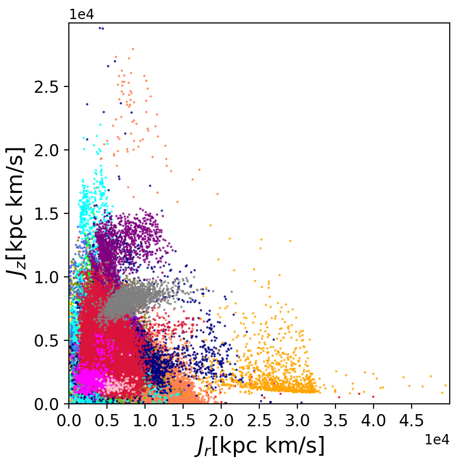
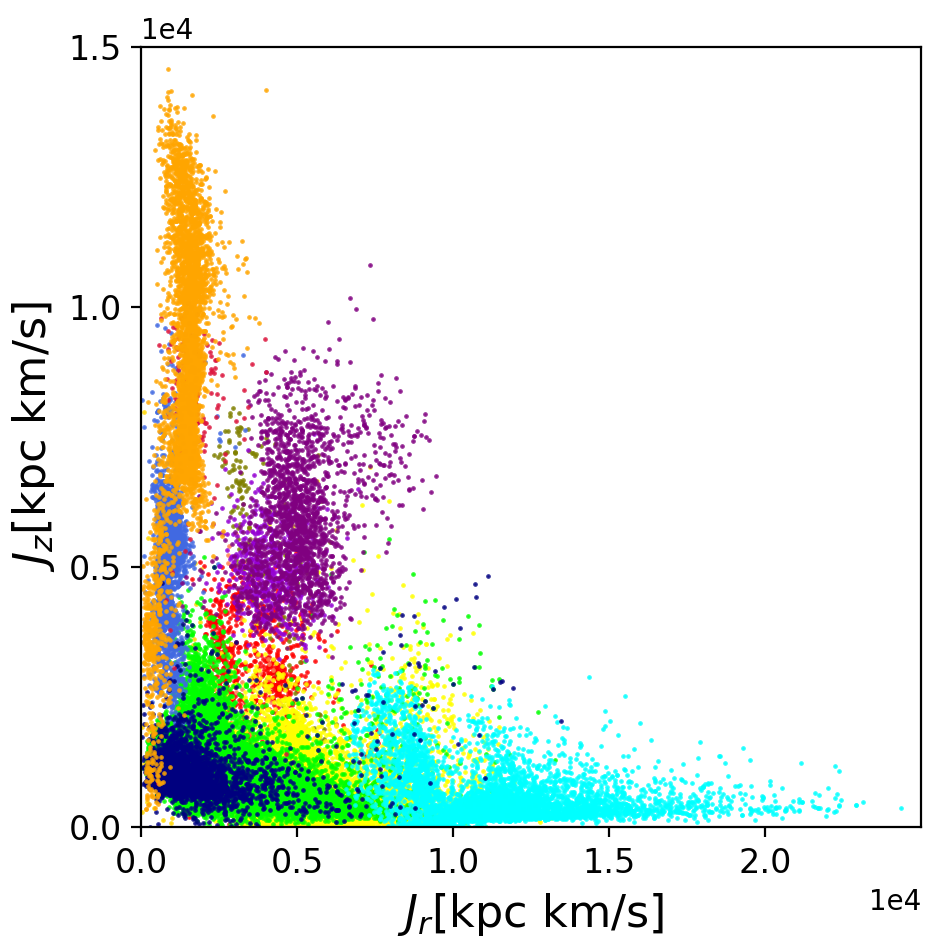
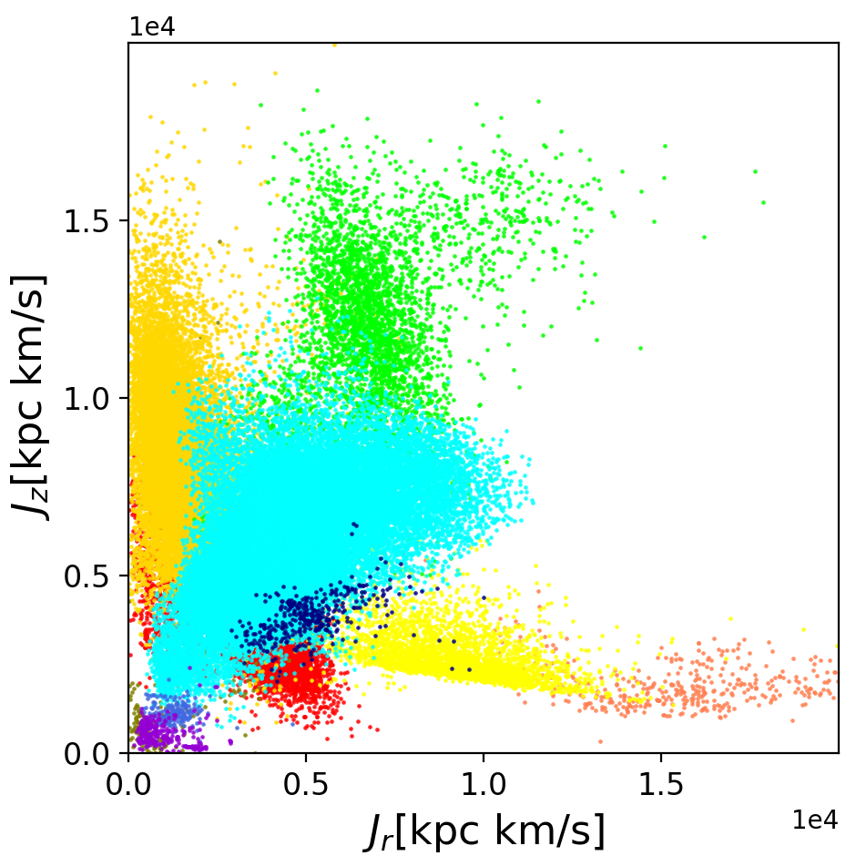
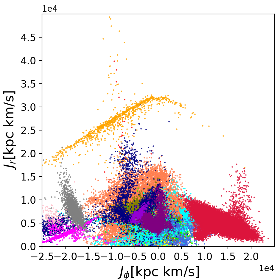
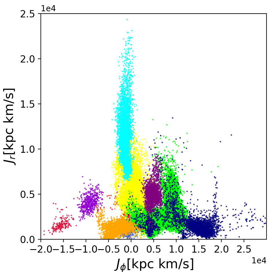
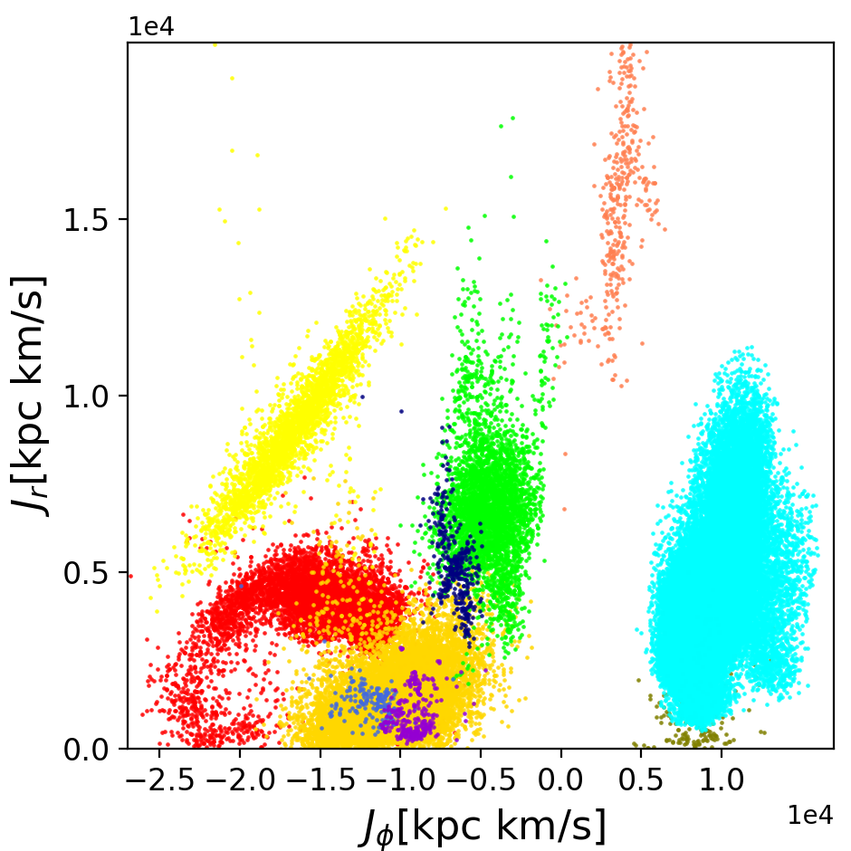
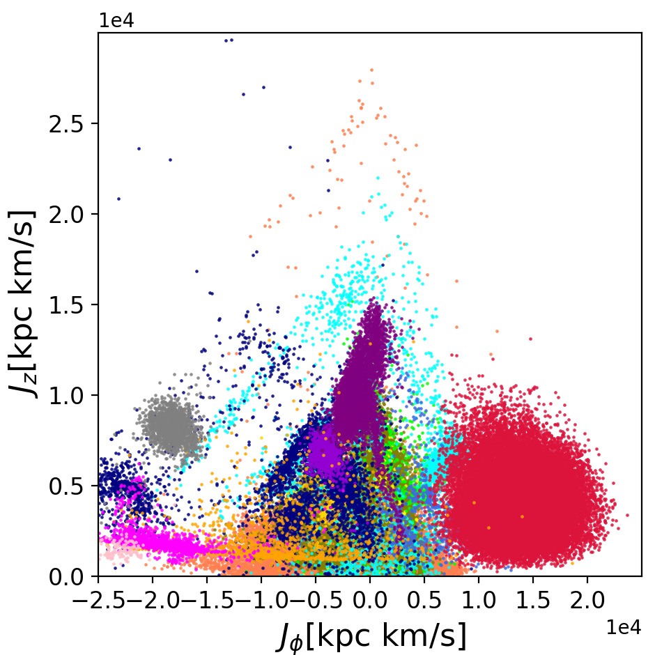
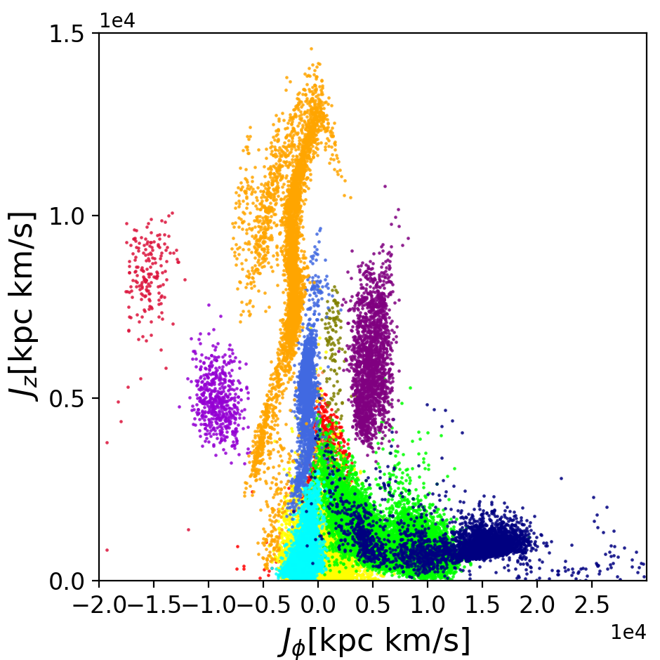
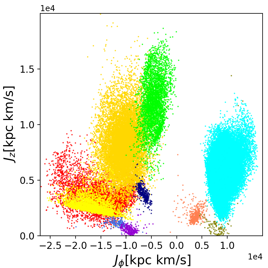
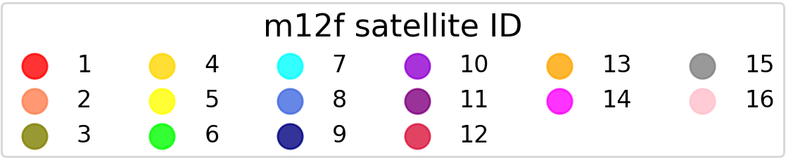
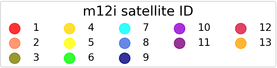
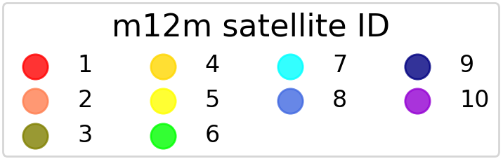
Figure 1: Two dimensional projections of actions $\{J_{r},J_{z},J_{\phi}\}$ for accreted star particles from 3 MW-like galaxies in FIRE-2 simulations. The three columns correspond to the three galaxies in FIRE-2 simulations: m12f, m12i and m12m, from left to right. Each accreted satellite identified from analyzing snapshots from the simulation is indicated by a different color.

.

3.2 Finding Clusters with Enlink

We apply algorithm Enlink  (Sharma & Johnston, 2009), a density-based hierarchical group finding algorithm capable of identifying structures of any shape and density in multi-dimensional datasets, to the action space variables $\{J_{r},J_{z},J_{\phi}\}$ for the 3 galaxies from FIRE-2. Enlink  is especially useful for astrophysical data as it can effectively detect groups which are not globular. Here we summarize the basic principles behind Enlink. For more details see Sharma & Johnston (2009).

1. Build a locally adaptive Mahalanobis (LAM) metric $\Sigma^{-1}(\mathbf{x})$. The distance squared between two data points $\mathbf{x_{i}}$ and $\mathbf{x_{j}}$ is defined as:

   $$s^{2}(\mathbf{x_{i}},\mathbf{x_{j}})=|\Sigma(\mathbf{x_{i}},\mathbf{x_{j}})|^{\frac{1}{d}}(\mathbf{x_{i}}-\mathbf{x_{j}})^{\intercal}\Sigma^{-1}(\mathbf{x_{i}},\mathbf{x_{j}})(\mathbf{x_{i}}-\mathbf{x_{j}})$$ (2)

   where $d$ is the dimension of data, $\Sigma^{-1}(\mathbf{x_{i}},\mathbf{x_{j}})=0.5(\Sigma^{-1}(\mathbf{x_{i}})+\Sigma^{-1}(\mathbf{x_{j}}))$. To build this LAM metric $\Sigma^{-1}(\mathbf{x})$, first divide the whole data set into regions with each region containing $(d+1)$ data points, and the particles in each region are distributed as uniformly as possible. Then calculate the local covariance matrix $\Sigma(\mathbf{x})$ of the data points in each region and smooth it so that this local matrix changes continuously and smoothly from region to region.

2. Calculate a local density $\rho(x)$ for each data point. For each data point, find $k$ nearest neighbours to it based on distance squared defined in Eq. (2). The size of neighborhood $k$ has a pre-defined default value in Enlink  : $k=10$. We have tried $k=5-20$, and the results are robust against the variation of $k$ in this range. Calculate density as:

   $$\rho(\mathbf{x_{j}})=\sum^{k}_{i=1}\frac{m_{i}}{h^{d}|\Sigma(\mathbf{x_{j}})|^{\frac{1}{2}}}W(\sqrt{(\mathbf{x_{i}}-\mathbf{x_{j}})^{\intercal}\Sigma^{-1}(\mathbf{x_{j}})(\mathbf{x_{i}}-\mathbf{x_{j}})}/h)$$ (3)

   where $h$ is the smoothing length corresponding to a given $k$, $d$ is the dimensionality of data space, $W$ is a kernel function to normalize the integral of density and $m_{i}$ is the mass of each particle.

3. Identify clusters based on density and preserve significant groups. We start building groups at local density peaks, and these groups grow by absorbing nearby points. Once two groups try to absorb a common particle, a saddle point is reached and the smaller group is absorbed into the bigger one as a subgroup (the subgroup is not canceled and still treated as a separate group). After all the (sub)groups are identified, the significance $S$ of each group is calculated:

   $$S=\frac{\ln(\rho_{\mathrm{max}})-\ln(\rho_{\mathrm{min}})}{\sigma_{\ln(\rho)}}$$ (4)

   where $\rho_{\mathrm{max}}$ and $\rho_{\mathrm{min}}$ are maximum and minimum densities in that group. $\sigma_{\ln(\rho)}$ is the standard deviation of log of densities in one group. We define the size of a satellite as the number of star particles it contains. We denote the minimum size of satellites we tracked by $N_{S}$. The minimum number of particles in a group, $N_{\mathrm{min}}$ , is chosen to be of the same order of magnitude as $N_{S}$. Then any group with number of particles lower than $N_{\mathrm{min}}$  would have its significance set to 0. For two intersecting groups, we compare their values of significance to a pre-determined threshold $S_{Th}$. If both groups have $S>S_{Th}$, then keep both of them. Otherwise, the one with lower $S$ is eliminated and its particles are absorbed into the group with higher $S$.

As can be seen from the description above, four parameters determine the result of cluster finding: size of neighborhood $k$, threshold significance $S_{Th}$, mass of each particle $m_{i}$ and minimum size of group $N_{\mathrm{min}}$. In this work, we neglect the mass of star particles, so all the $m_{i}$ is set to 1. Three other parameters have their default values pre-defined in the Enlink  program. During our runs, $k$ and $S_{Th}$ are varied slightly around their default values and $N_{\mathrm{min}}$  is chosen to be in the same order of magnitude as the minimum size of satellites, so that the number of groups that the algorithm yields is close to the number of accreted satellites in a galaxy.

Groups that were identified by Enlink  with $k=10$, $N_{\mathrm{min}}$$=300$ and $S_{Th}$ at its default value for the three galaxies from the FIRE-2 simulations are shown in Fig. 2. The minimum number of star particles in each of the satellites in the three galaxies is around 150 (corresponding to a minimum stellar mass of around $6.0\times 10^{5}{\rm\,M_{\odot}}$), so a reasonable value for $N_{\mathrm{min}}$  would seem to be 150. With $N_{\mathrm{min}}$$=150$, many small random groups emerge in all three galaxies. With $N_{\mathrm{min}}$$=300$ the identification of large and clear satellites is not affected in m12f and m12m, but in m12i, a satellite with size 184 (located in action space at around $J_{\phi}=-12000\mathrm{kpc\times km/s},J_{z}=8000\mathrm{kpc\times km/s},J_{r}=2000\mathrm{kpc\times km/s}$) cannot be identified. However, since many small spurious groups that emerge at $N_{\mathrm{min}}$$=150$ make it harder to identify the large and clear satellites, we keep $N_{\mathrm{min}}$$=300$, corresponding to a minimum stellar mass of around $1.2\times 10^{6}{\rm\,M_{\odot}}$ for groups found by Enlink .

In applications to observational data, since the sizes of datasets are expected to be much larger and the number of accreted satellites is completely unknown, these 4 parameters should be determined carefully. It is also likely that one satellite could be split into multiple groups by cluster analysis (Yuan et al., 2020). Adding additional information, such as metallicity or abundances of specific elements (e.g. Ca, N, Fe, Eu, Sanderson et al., 2017; Roederer et al., 2018) can help to confirm the identification of a satellite or identify subcomponents of a single satellite, but this is beyond the scope of this paper. In this paper, we are testing how well cluster analysis in the action space alone can perform under optimum conditions: perfect knowledge of all 6 phase space coordinates, accurate representation of the galactic potential, and prior insights into the optimum values of parameters like $N_{\mathrm{min}}$. These simplifying assumptions enable us to assess how well cluster analysis can perform in the best-case scenario.

3.3 Metrics to Assess Identification of Satellites by Clusters

In order to quantify the ability of Enlink  to identify accreted satellites in action space, we define three matrices: $R_{ij}$, $P_{ij}$ and $M_{ij}$; and four quantities based on these matrices: recovery, purity, merit and contrast. We refer to the clusters identified by Enlink  as “groups”. The number of star particles contained in a group is called the size of the group. In order to quantify the degree to which a group identified by Enlink  matches one of the original accreted satellites we also define the “best recovery group” (similarly for purity, merit) and best fit group. Based on recovery, purity, merit and best fit group, we select out the “well-recovered satellites”.

1. Three matrices $R_{ij},P_{ij},M_{ij}$: The $ij$ component of these three matrices describes the similarity between satellite $j$ and group $i$:

   $$R_{ij} = \frac{\mathrm{number\leavevmode\nobreak\ of\leavevmode\nobreak\ particles\leavevmode\nobreak\ shared\leavevmode\nobreak\ by\leavevmode\nobreak\ satellite}\leavevmode\nobreak\ \mathit{j}\leavevmode\nobreak\ \mathrm{and\leavevmode\nobreak\ group}\leavevmode\nobreak\ \mathit{i}}{\mathrm{number\leavevmode\nobreak\ of\leavevmode\nobreak\ particles\leavevmode\nobreak\ in\leavevmode\nobreak\ satellite}\leavevmode\nobreak\ \mathit{j}},$$

   $$P_{ij} = \frac{\mathrm{number\leavevmode\nobreak\ of\leavevmode\nobreak\ particles\leavevmode\nobreak\ shared\leavevmode\nobreak\ by\leavevmode\nobreak\ satellite}\leavevmode\nobreak\ \mathit{j}\leavevmode\nobreak\ \mathrm{and\leavevmode\nobreak\ group}\leavevmode\nobreak\ \mathit{i}}{\mathrm{number\leavevmode\nobreak\ of\leavevmode\nobreak\ particles\leavevmode\nobreak\ in\leavevmode\nobreak\ group}\leavevmode\nobreak\ \mathit{i}},$$

   $$M_{ij} = R_{ij}\times P_{ij}$$

2. Recovery, purity, merit: For satellite $k$, the maximum values of $R_{ik},P_{ik}$ and $M_{ik}$ are called the recovery ($r_{k}$), purity ($p_{k}$) and merit ($m_{k}$) of this satellite:

   $$r_{k} = \mathrm{max}_{i}\{R_{ik}\},{\rm for\,i\,in\,range\,of\,group\,indices}$$

   $$p_{k} = \mathrm{max}_{i}\{P_{ik}\},{\rm for\,i\,in\,range\,of\,group\,indices}$$

   $$m_{k} = \mathrm{max}_{i}\{M_{ik}\},{\rm for\,i\,in\,range\,of\,group\,indices}$$

3. Best recovery, purity, merit group and best fit group: For satellite $k$, the group which yields $r_{k}$ is called the “best recovery group”, and likewise $p_{k}$ and $m_{k}$ define the “best purity group” and “best merit group” of satellite $k$, respectively. If a group is both the “best recovery group” and the “best purity group” of satellite $k$, then it is defined as the “best fit group” of satellite $k$.

4. Contrast: To compare the size of satellite $k$ and its best fit group, we define contrast ($c_{k}$) as:

   $$c_{k}=\frac{r_{k}-p_{k}}{\sqrt{r_{k}p_{k}}}$$ (5)

   where $r_{k}$ and $p_{k}$ are recovery and purity of satellite $k$. Note contrast is only defined for a satellite with a best fit group. When $c_{k}$ is positive, satellite $k$ is smaller than its best fit group (the group contains contaminants - i.e. stars that were not originally part of the satellite), and when $c_{k}$ is negative, satellite $k$ is larger than its best fit group (not all of the members of the satellite have been identified as group members).

5. Well-recovered satellite: If the recovery, purity and merit of a satellite are all greater than 0.5 and this satellite has a best fit group, then this satellite is called well-recovered or is said to have a high identifiability score. A satellite that is not well-recovered is called poorly-recovered.

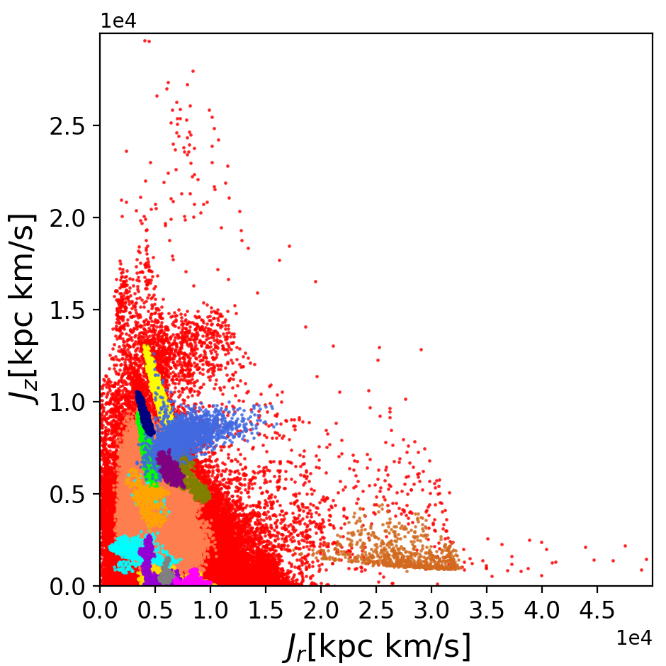
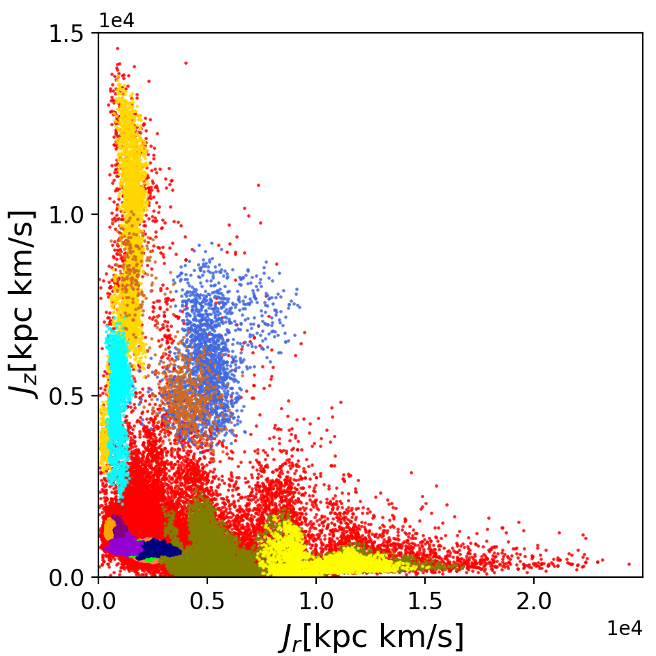
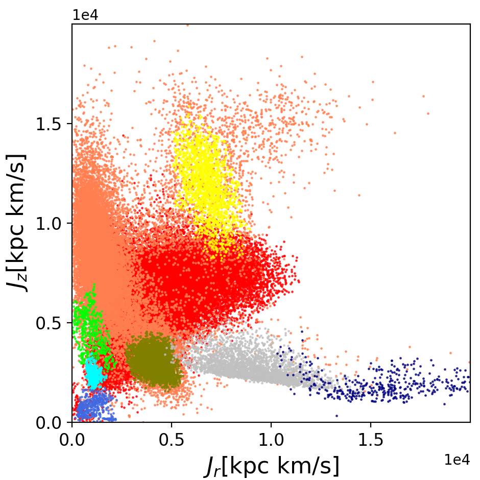
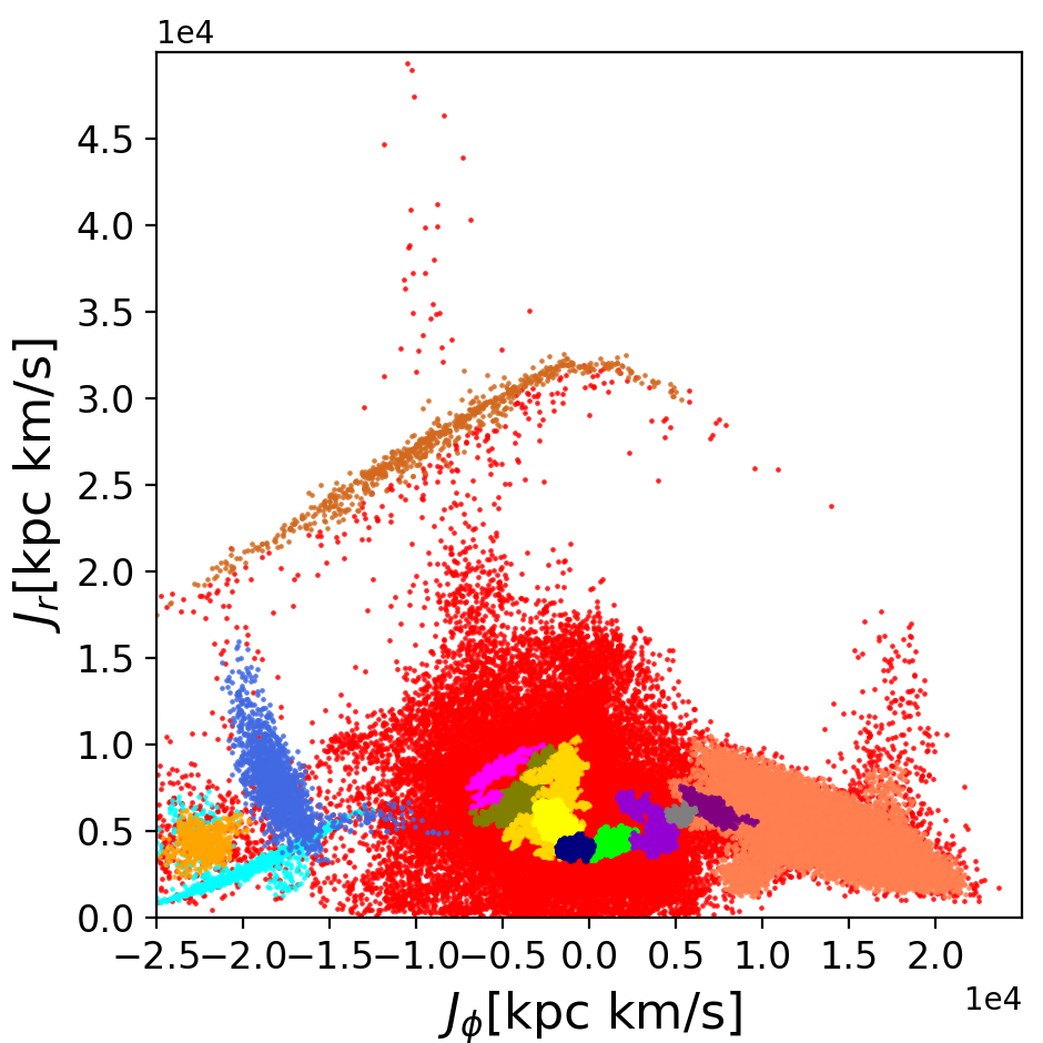
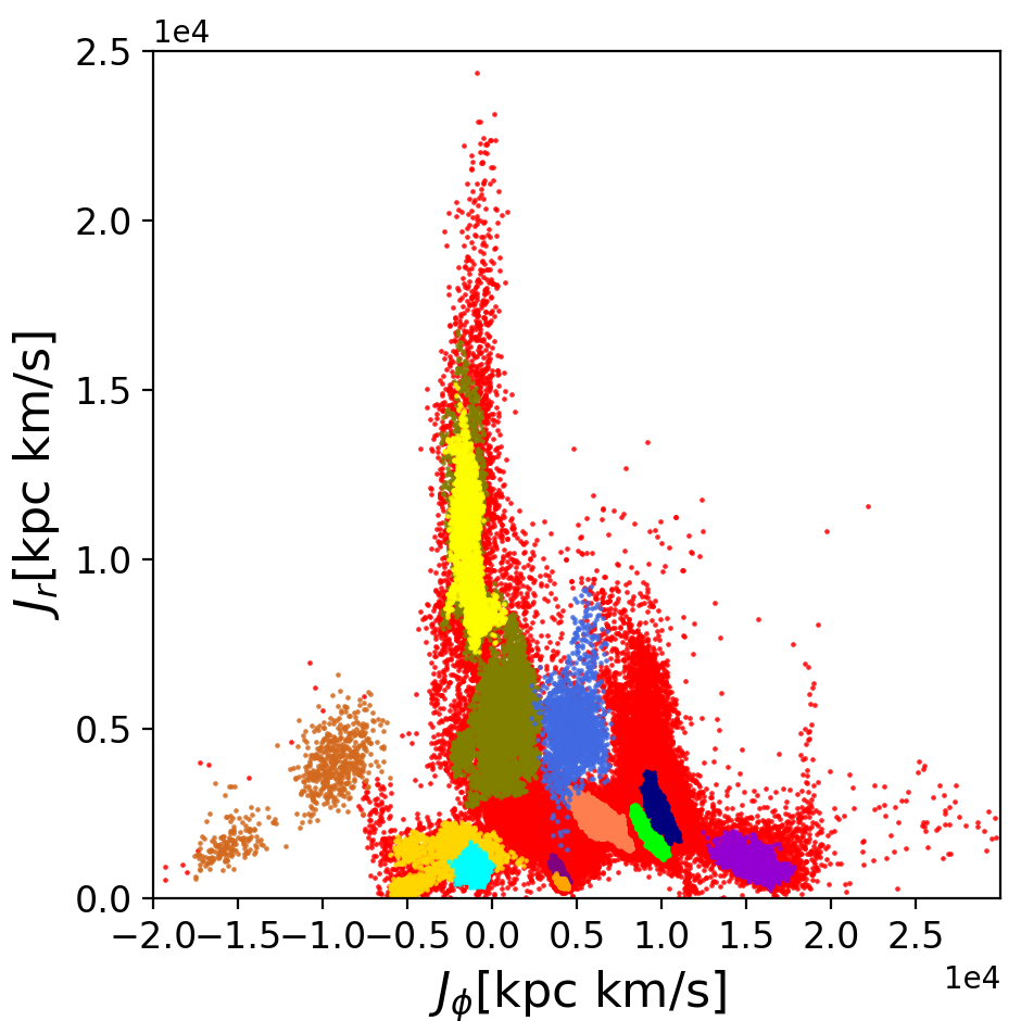
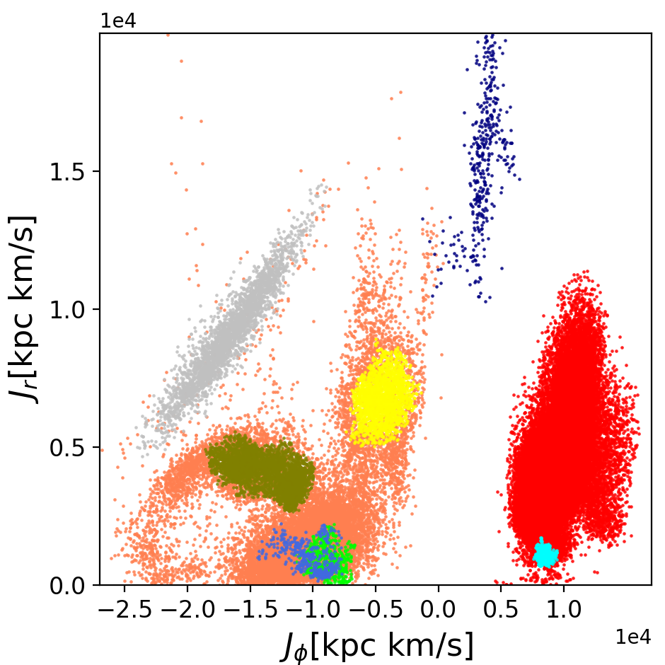
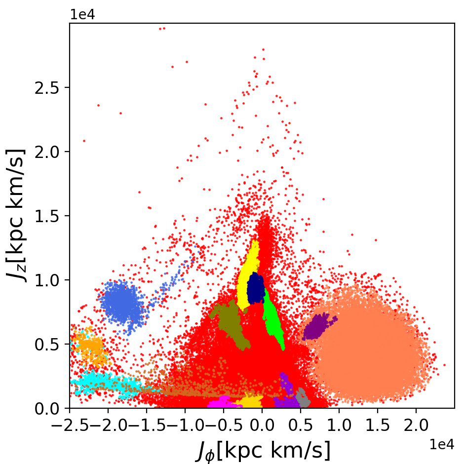
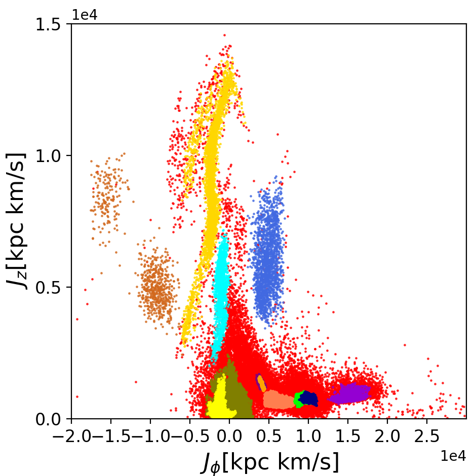
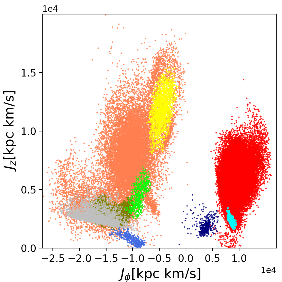
Figure 2: Same as Fig. 1, but with substructures identified by Enlink  to see how well Enlink  can reproduce the actual satellites in the simulations as shown in Fig. 1. Particles from different groups identified by Enlink  are indicated by different colors. Results plotted here are obtained from Enlink  runs with size of neighbourhood $k=10$, minimum group size $N_{\mathrm{min}}=300$ and significance threshold $S_{Th}$ at its default value.

.

4 Results

We do a cluster analysis with Enlink  on actions $\{J_{r},J_{z},J_{\phi}\}$ of accreted star particles from three MW-like galaxies in FIRE-2 simulations. In Section 4.1, we calculate the values of recovery, purity, merit and contrast for each satellite in three galaxies to evaluate how well these satellites are recovered by Enlink. We study the distribution of well-recovered satellites on the $M_{\mathrm{tot}}$-$T_{\mathrm{infall}}$  plane and $M_{\rm stellar}$-$T_{\mathrm{infall}}$  plane, and find the boundaries in $M_{\mathrm{tot}}$  $M_{\rm stellar}$ and $T_{\mathrm{infall}}$ values that separate well-recovered and poorly-recovered satellites by the classification tree method. We also investigate the relation between significance of a group and the identification power of this group (that is, whether this group corresponds to a well-recovered satellite or not). In Section 4.2, we include certain percentages of  in situ  stars into the input data set for cluster analysis. We pick out the well-recovered satellites which are identified when  in situ   star particles are absent. Calculate the values of merit of these satellites under different  in situ  star contamination ratios and demonstrate the robustness of the identification of these satellites under the contamination of  in situ  star particles.

4.1 Cluster Analysis on Accreted Star Particles

We apply Enlink  to the actions $\{J_{r},J_{z},J_{\phi}\}$ for accreted star particles from the MW-like galaxies m12f, m12i and m12m in FIRE-2 simulations. In a manner similar to Fig. 1 three projections of the actions for accreted star particles $\{J_{r},J_{\phi},J_{z}\}$ are shown in Figure 2, but now the color coding corresponds to the individual groups that are identified by Enlink. The legend in the bottom row now indicates the color coding for the individual groups identified. A comparison with Fig. 1 shows visually that while in m12i and m12m the number of groups identified is one larger than the number of satellites., in m12f only 15 groups (of 16 satellites) are identified. Overall however, there is an excellent correspondence between the groups identified by Enlink  and the original satellites seen in Fig. 1.

Fig. 3 shows the values of recovery, purity, merit and contrast of 39 satellites in the three simulated galaxies m12f, m12i and m12m, on a $M_{\mathrm{tot}}$  vs. $T_{\mathrm{infall}}$ plot. Each symbol corresponds to one accreted satellite and symbols are color coded by the value of their recovery (panel a), purity (panel b), merit (panel c) and contrast (panel d), with red colored points indicating better results. In panels a, b, and c, satellites are also shape coded by whether their best recovery group match their best purity group (triangle) or not (circle) (in other words, whether the satellite has a best fit group (triangle) or not (circle)). White numbers indicate the group ID (as shown in Fig. 2) signifying best recovery (panel a), best purity (panel b), best merit (panel c) or best fit (panel d) for each satellite. A white letter associated with each data point indicates which galaxy this satellite is from: ‘f’ for ‘m12f’, ‘i’ for ‘m12i’ and ‘m’ for ‘m12m’. Among the 39 satellites, 14 of them are “well-recovered” (their values of recovery, purity and merit are larger than 0.5 and they have best fit groups), while 25 of them are poorly-recovered. With $T_{\mathrm{infall}}$  and $\log_{10}(M_{\rm tot}/{\rm\,M_{\odot}})$ as inputs, we grow a classification tree to predict whether a satellite is well-recovered or not. (For a brief introduction to classification tree method, see Appendix A) The boundaries that the classification tree finds out are: $T_{\mathrm{infall}}$= 7.1 Gyr ago and $M_{\mathrm{tot}}$= $10^{8.6}{\rm\,M_{\odot}}$, which are shown as vertical and horizontal blue dashed lines in Fig. 3. 91% (10/11) of the satellites in the region bounded by $M_{\mathrm{tot}}$$>4.0\times 10^{8}{\rm\,M_{\odot}}$ and $T_{\mathrm{infall}}$$<7.1$ Gyr ago are “well-recovered” satellites. Of the satellites outside this region, 86% of the sample (24/28) are poorly-recovered. Three satellites in galaxy m12i (marked by 3i, 4i and 7i on the plot) fell into the host galaxy far more than 7.1 Gyr ago ($T_{\mathrm{infall}}$= 9.08-10.33 Gyr ago), but are still well-recovered. This can be attributed to the unique dynamic history of galaxy m12i. See Section 5 for more discussion. Group 1 in each galaxy is the “best” group of many satellites, because Group 1 is the largest group and contains star particles from many “poorly-recovered” satellites. Group 1 in each of the galaxies can be considered as the “background” group. Panel d plots the contrast of satellites, shape coded by whether the contrast is positive (diamond) or negative (square). Only the satellites with a best fit group are plotted in panel d. Note that a positive contrast means that a satellite is smaller than its best fit group, and a negative contrast means the opposite. Most of the values of contrast are close to 0, with a few extremely large values (above 20). These extremely large values belong to satellites with Group 1 as best fit group, indicating that Group 1 is much larger than these satellites, consistent with the fact that Group 1 contains star particles from many satellites and is the background group. The values of contrast of “well-recovered” satellites are close to 0, meaning the number of particles in these satellites is similar to that in their best groups.

Similar to Fig. 3, in Fig. 4 we plot the values of recovery, purity, merit and contrast of 39 satellites in the three simulated galaxies m12f, m12i and m12m, on the $M_{\rm stellar}$ vs. $T_{\mathrm{infall}}$ plane. The color code, shape code and the meaning of the white numbers/letters are the same as those in Fig. 3. The boudaries separating well-recovered and poorly-recovered satellites found by the classification tree method in the $M_{\rm stellar}$ vs. $T_{\mathrm{infall}}$ plane are: $M_{\rm stellar}=1.2\times 10^{6}{\rm\,M_{\odot}}$ and $T_{\mathrm{infall}}$= 7.1 Gyr ago, marked by the horizontal and vertical blue dashed lines in the four panels. The $T_{\mathrm{infall}}$  boundaries found in $M_{\mathrm{tot}}$  vs. $T_{\mathrm{infall}}$ and $M_{\rm stellar}$ vs. $T_{\mathrm{infall}}$ planes agree with each other. 91% (10/11) of the satellites with $M_{\rm stellar}$ greater than $1.2\times 10^{6}{\rm\,M_{\odot}}$ and fell into the halo less than 7.1 Gyr ago are well-recovered by Enlink.

In Section 3.2, we find that 150 star particles are corresponding to $M_{\rm stellar}\approx 6\times 10^{5}{\rm\,M_{\odot}}$, so setting $N_{\rm min}=300$ is equivalent to setting the lower bound of $M_{\rm stellar}$ to be around $1.2\times 10^{6}{\rm\,M_{\odot}}$ for groups found by Enlink . Any group with less stellar mass than $1.2\times 10^{6}{\rm\,M_{\odot}}$ (number of particles smaller than $N_{\rm min}=300$) will not be found by Enlink  under our choice of $N_{\rm min}$. This lower bound in $M_{\rm stellar}$ agrees with the $M_{\rm stellar}=1.2\times 10^{6}{\rm\,M_{\odot}}$ boundary for well-recovered satellites. This agreement raises a caveat that the boundary on $M_{\rm stellar}$ (probably also on $M_{\mathrm{tot}}$) might be an artifact due to a particular choice of $N_{\rm min}$.

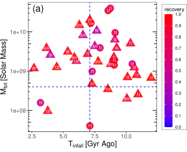
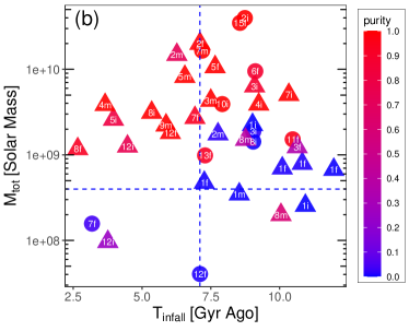
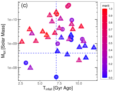
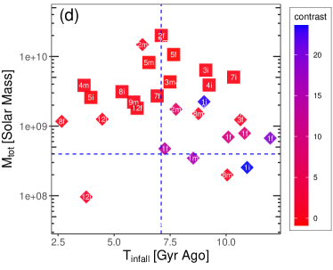
Figure 3: 39 satellites in 3 MW-like galaxies from the FIRE-2 simulations plotted on the $M_{\mathrm{tot}}$  vs. $T_{\mathrm{infall}}$  plane. Data points are color coded by the recovery (panel a), purity (panel b), merit (panel c) or contrast (panel d), with red points indicating better results in all panels. The white number on each symbol indicates the group ID (as shown in Fig. 2) of the “best recovery” (panel a), “best purity” (panel b), “best merit” (panel c) and “best fit” (panel d) group corresponding to each satellite. The white letters associated with each data point indicates which galaxy each satellite is from: “f” for “m12f”, “i” for “m12i” and “m” for “m12m”. Group 1 in all three galaxies is the “best” group of many satellites because it is the largest group, as shown in Fig. 2, and is generally considered as the “background”. A satellite is marked as a triangle if it has a “best fit group” and as a circle otherwise. Satellites are from the analysis of simulation data in Section 2, and groups are identified by Enlink. In panel d, only satellites with best fit groups are plotted, and shapes indicate whether the contrast is positive (diamond) or negative (square). Among the 39 satellites, 14 of them are well-recovered and 25 of them are poorly recovered. The vertical and horizontal dashed lines mark $M_{\mathrm{tot}}$$=4.0\times 10^{8}{\rm\,M_{\odot}}$ and $T_{\mathrm{infall}}$= 7.1 Gyr ago, which are the boundaries identified by the classification tree method. 91% (10/11) of the satellites with $M_{\mathrm{tot}}$  greater than $4.0\times 10^{8}{\rm\,M_{\odot}}$ and fell into the halo less than 7.1 Gyr ago are well-recovered by Enlink.

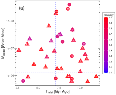
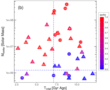
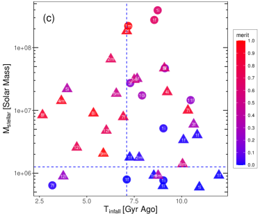
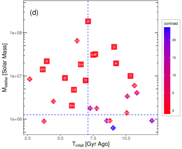
Figure 4: Same as Fig. 3, but the y axes of these plots are labeling $M_{\rm stellar}$. The vertical and horizontal dashed lines mark $M_{\rm stellar}=1.2\times 10^{6}{\rm\,M_{\odot}}$ and $T_{\mathrm{infall}}$= 7.1 Gyr ago, which are the boundaries separating well-recovered and poorly-recovered satellites identified by the classification tree method. 91% (10/11) of the satellites with $M_{\rm stellar}$ greater than $1.2\times 10^{6}{\rm\,M_{\odot}}$ and fell into the halo less than 7.1 Gyr ago are well-recovered by Enlink.

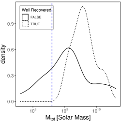
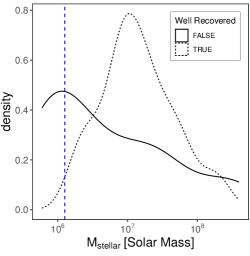
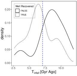
Figure 5: Kernel density plots of 39 satellites from three galaxies in $M_{\mathrm{tot}}$(left), $M_{\rm stellar}$ (middle) and $T_{\mathrm{infall}}$  (right). The three blue vertical dashed lines label the boundaries in Fig. 3 and Fig. 4: $M_{\mathrm{tot}}$$=4.0\times 10^{8}{\rm\,M_{\odot}}$ (left), $M_{\rm stellar}=1.2\times 10^{6}{\rm\,M_{\odot}}$ (middle) and $T_{\mathrm{infall}}$$=7.1$ Gyr ago (right). In all three panels, the dotted density curve labels the well-recovered satellites, while the solid curve labels the poorly-recovered satellites. In the left panel, both the dotted and solid density curves peak above $M_{\mathrm{tot}}$$=4.0\times 10^{8}{\rm\,M_{\odot}}$, with the dotted curve peaking at a higher $M_{\mathrm{tot}}$, indicating that well-recovered satellites tend to be more massive. In the middle panel, the dotted curve peaks at a higher $M_{\rm stellar}$, indicating that well-recovered satellites tend to be have more stellar mass. In the right panel, the peaks of dotted and solid curves are on the two sides of $T_{\mathrm{infall}}$$=7.1$ Gyr ago

.

To appreciate how well the boundaries $M_{\mathrm{tot}}$= $4.0\times 10^{8}{\rm\,M_{\odot}}$, $M_{\rm stellar}=1.2\times 10^{6}{\rm\,M_{\odot}}$ and $T_{\mathrm{infall}}$= 7.1 Gyr ago work in separating out well-recovered satellites, we show three kernel density plots of 39 satellites from three galaxies in $M_{\mathrm{tot}}$(left), $M_{\rm stellar}$ (middle) and $T_{\mathrm{infall}}$(right) in Fig. 5. In all three panels, the dotted density curve represents well-recovered satellites, while the solid curve represents poorly-recovered satellites. The two curves are normalized separately. The vertical dashed lines in three panels show the boundaries in Fig. 3 and Fig. 4: $M_{\mathrm{tot}}$= $4.0\times 10^{8}{\rm\,M_{\odot}}$, $M_{\rm stellar}=1.2\times 10^{6}{\rm\,M_{\odot}}$ and $T_{\mathrm{infall}}$= 7.1 Gyr ago. In the left panel, the dotted curve peaks at a higher $M_{\mathrm{tot}}$  than the solid curve, indicating that well-recovered satellites tend to be more massive. However, the peaks of both curves are greater than $4.0\times 10^{8}{\rm\,M_{\odot}}$, indicating that the boundary in $M_{\mathrm{tot}}$  alone cannot distinguish between well-recovered and poorly-recovered satellites. In the middle panel, the solid curve peaks at a lower value than the dotted curve, indicating that well-recovered satellites tend to have more stellar mass than poorly-recovered ones. The peak of the solid curve is close to the $M_{\rm stellar}=1.2\times 10^{6}{\rm\,M_{\odot}}$ boundary, indicating that $M_{\rm stellar}$ alone cannot distinguish well-recovered satellites and poorly-recovered satellites either. In the right panel, the peaks of dotted and solid density curves are on the two sides of the $T_{\mathrm{infall}}$  boundary, justifying the boundary $T_{\mathrm{infall}}$= 7.1 Gyr ago.

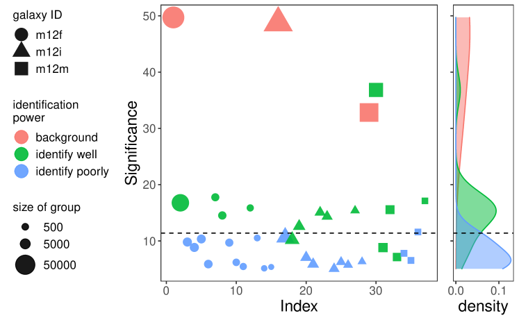
Figure 6: The values of significance of 37 (34 non-background+3 background) groups identified by Enlink  in 3 MW-like galaxies (as shown in Fig. 2) are plotted. “Index” is a number between 1 and 37 to label each group. The size of a data point is proportional to the number of particles in the group. Groups from galaxies m12f, m12i and m12m are marked by circles, triangles and squares, respectively. The colour of a data point indicates whether the groups is a background group (salmon), corresponds to a well-recovered satellite (green) or does not identify any satellite (blue). A kernel density plot is attached on the right hand side of the scatter plot. The black dashed line labeling the valley between green and blue curve peaks shows the cutoff in significance for groups corresponding to well-recovered satellites. The cutoff value in significance for groups corresponding to well-recovered satellites is 11.4, the 66th percentile of the significance of non-background groups.

We have seen that massive satellites fell into MW-like galaxies relatively recently can be reliably recovered by cluster analysis in action space with Enlink. In future applications to observational data it will be necessary to use a statistical metric provided by Enlink  to determine which groups are most likely to correspond to real satellites. The variable significance, assigned by Enlink  to each group and calculated by Equation (4), is a good indicator of whether a group corresponds to a real satellite or not. In Fig. 6 we plot the values of significance of 34 non-background groups and 3 background groups. The size of a data point is proportional to the number of particles in the group, while the shape shows which galaxy this group is from, and the colour indicates whether the group is a background group (salmon), identifies a satellite well (green) or does not identify a single satellite (blue). A kernel density plot is attached on the side of the scatter plot. The green curve showing the distribution of significance peaks at a higher significance than the blue curve. The black dashed line shows the valley between the green and blue peaks. This valley, located at significance = 11.4 or the 66th percentile of the values of significance of the non-background population, is the cutoff in significance for groups corresponding to well-recovered satellites. Note the cutoff in significance here should not be confused with $S_{Th}$ in Section 3.2. Among 12 non-background groups with significance above the cutoff, 11 of them are corresponding to “well-recovered” satellites. This result implies that with the results of Enlink  cluster analysis in action space alone (i.e. no other information on satellites, and ignoring the largest group identified by Enlink  assuming it to be “background”), groups with higher significance than 66% of groups found by Enlink  are very likely to be corresponding to true satellites.

4.2 The Effect of In-situ Stars

Besides accreted stars, cosmological hydrodynamical simulations predict that  in situ  stars may also contribute to a significant part of the halo star population in a galactic halo. As mentioned earlier, the fraction of  in situ  halo stars is highly uncertain but estimates in the MW (Bell et al., 2008; Naidu et al., 2020) suggest it could be as small as 5%, while studies of resolved halo stellar populations in external galaxies find that the properties of these halo stars are consistent with being purely accreted (Harmsen et al., 2017). Recent work (Naidu et al., 2020) shows that in the MW halo, the relative fraction of  in situ  stars drops below 0.5 when $|Z_{gal}|>5\mathrm{kpc}$, where $|Z_{\mathrm{gal}}|$ is the distance from the disk plane. We also note that over 95% of the accreted star particles in the three MW-like galaxies have $|Z_{\mathrm{gal}}|>5\mathrm{kpc}$. Therefore to study the effects of  in situ  stars on the robustness of satellite identification by cluster analysis in the action space, we build numerous mock data sets with  in situ  contamination ratios equaling 0.1, 0.2, 0.3, 0.4 and 0.5 (where contamination ratio of 0.5 implies that 50% of the halo star sample consists of  in situ  stars) in three MW-like galaxies by randomly sampling the  in situ  star particles with $|Z_{\mathrm{gal}}|>5\mathrm{kpc}$. We then calculate the actions $\{J_{r},J_{z},J_{\phi}\}$ and do cluster analysis with Enlink  in the action space on these “contaminated” data sets. We pick out the well-recovered satellites in Section 4.1 and study their values of merit at different contamination ratios. To reduce the effect of the randomness in sampling the  in situ  star particles, for every contamination ratio in each galaxy, we repeat the selection of the  in situ  “contaminant” population 100 times, randomly picking the same fraction of  in situ  stars each time. We then generate the value of merit for each well-recovered satellite from each data set. Each well-recovered satellite at a contamination ratio then has 100 values of merit. We calculate the average and standard deviation of those 100 values. If the previously well-recovered satellite doesn’t have a best fit group in one data set (i.e., the best recovery group doesn’t match with the best purity group), then the merit of that satellite in that run is set to 0.

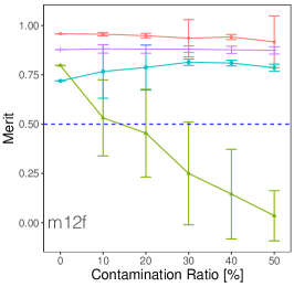
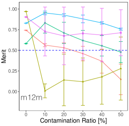
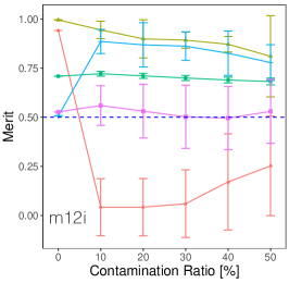
Figure 7: Values of merit of well-recovered satellites in three galaxies (m12f, m12i, m12m from left to right) at different  in situ  contamination ratios. Each differently colored line corresponds to one well-recovered satellite in each galaxy (the well-recovered satellites in three galaxies are summarized in Fig. 3). The values of merit come from the average of 100 runs and the error bars show the standard deviations. A blue dashed line in 3 panels shows merit=0.5, the threshold of “well-recovered” objects. 64% (9/14) of the well-recovered satellites have values of merit greater than 0.5 at all contamination ratios, being robust against the contamination from  in situ  star particles. As the contamination ratio increases, the values of merit of some satellites drop below 0.5. These “vulnerable” satellites have higher standard deviations in merit than other robust satellites, showing that they are more affected by the randomness of picking  in situ  star particles. Despite a few exceptions, there is a general trend that the merit decreases as the contamination ratio increases. The robustness of well-recovered satellites indicates that Enlink  can recover most of the well-recovered satellites when  in situ    star particles are in the data set.

Fig. 7 illustrates the change of values of merit of well-recovered satellites in three MW-like galaxies (as shown in Section 4.1) as the contamination ratio increases from 0 to 0.5. Each data point and error bar in the figure shows the average and standard deviation of results of 100 runs, respectively. Lines of different colors correspond to different well-recovered satellites. 64% (9/14) of the satellites are robust against the contamination from  in situ  star particles, as their values of merit are above 0.5 at all contamination ratios. Other satellites fade away from the identification of Enlink  (merit $<0.5$) as the contamination ratio increases. The standard deviation of the merit of these satellites are also higher than their robust companions, showing that they are more vulnerable under the random draw of the  in situ  star particles. Besides a few satellites, as expected, most (79%, 11/14) of the values of merit generally decrease as the contamination ratio increases.

5 Discussion and Conclusions

Inspired by the principle of conservation of orbital actions, we use cluster analysis in action space to find accreted satellites with accreted star particles in three MW like galaxies in the FIRE-2 cosmological hydrodynamical simulations. We summarize the main findings of our work below:

1. Classification tree method finds the boundaries separating well-recovered and poorly-recovered satellites to be $T_{\mathrm{infall}}$= 7.1 Gyr ago and $M_{\mathrm{tot}}$= $4.0\times 10^{8}{\rm\,M_{\odot}}$ (or $M_{\rm stellar}=1.2\times 10^{6}{\rm\,M_{\odot}}$) (see Fig. 3 and Fig. 4). We note however, that the boundary in $M_{\rm stellar}$ coincides with the minimum mass of groups that Enlink  is set up to identify, determined by $N_{\rm min}$. This coincidence implies that the mass boundary could be an artifact of the choice of $N_{\rm min}$.
   The three galaxies have slightly different infall time and mass boundaries for reliable detection. For example, galaxy m12i has 3 well-recovered satellites which fell into the hosting halo more than 7.1 Gyr ago. This difference could be due to the distinct dynamical/evolutionary histories of the galaxies. Fig. 8 shows the offset angle, $\Delta\theta$, between the angular momentum vector of the disk at a given look-back time and the present time ($z=0$) as a function of look-back time for each of the three galaxies analyzed in this paper. The disk stars at each look-back time are defined as star particles that are within 30 kpc and also have formation distance within 30 kpc from the center of the host galaxy. The graph shows that the direction of the angular momentum vector often changes suddenly and through large angles (presumably due to merger events) for look back time $>8$ Gyr ago. Santistevan et al. (2021) shows that many of the changes in this $\Delta\theta$ correlate with major gas-rich mergers. In particular, galaxies m12f and m12m experienced numerous chaotic changes in $\Delta\theta$ until 8 Gyr ago, after which $\Delta\theta$ changed much more slowly and steadily. The slow change in $\Delta\theta$ implies the gravitational potentials of these two galaxies have changed adiabatically over the last 8 Gyrs, and therefore orbital actions of particles should be reasonably well conserved. The conservation of orbital actions implies that satellites accreted less than 8 Gyr ago should be found clustered in action space at $z=0$. This “8 Gyr ago” time limit for finding satellites clustered in action space is in agreement with the time boundary for good recovery that we found in Section 4. $\Delta\theta$ of galaxy m12i changes more smoothly compared with the other 2 galaxies, so it is expected that satellites accreted a long time ago would remain clustered in action space. This is in agreement with the fact that three satellites in this galaxy with $T_{\mathrm{infall}}$  $>9$ Gyr ago are still well-recovered by Enlink. In our Milky Way galaxy, Gaia Enceladus, which has $T_{\mathrm{infall}}$$\approx$ 10 Gyr ago and progenitor stellar mass $6\times 10^{8}{\rm\,M_{\odot}}$ (Helmi et al., 2018), can still be recovered in phase space. The recovery of this massive substructure which fell into the Milky Way a long time ago indicates that the Milky Way might evolve smoothly from relatively early on, like m12i in the FIRE-2 simulations.

2. The value of significance of a group shows a high correlation with the identification power of this group (see Fig. 6). Of the groups with high significance ($>$11.4, 66th percentile of the significance of non-background groups in three galaxies), most (92%, 11/12) correspond to the well-recovered satellites. This implies that if cluster analysis in action space is applied to observational data, this significance assigned by Enlink  can help us determine which groups are most likely to correspond to true accreted satellites.

3. Most of the well-recovered satellites are robust against contamination of  in situ  star particles (see Fig. 7). 64% (9/14) of the well-recovered satellites in Section 4.1 stay well-recovered (with merit $>0.5$) at 5 different contamination ratios (0.1, 0.2, 0.3, 0.4 and 0.5), where contamination ratio is the percentage of  in situ    star particles in the data set of one galaxy. The satellites which fail to be identified by Enlink  in the presence of contamination have higher standard deviations in merit, indicating that they are more sensitive to the randomness in picking  in situ  stars. This robustness against contamination from  in situ  star particles indicates that it will be possible to apply cluster analysis in action space to observation data, even if there is significant contamination from  in situ  stars. This is reassuring since the expected fraction of  in situ  stars in the MW ( 5%) is at the low end of the contamination fractions we have experimented with.

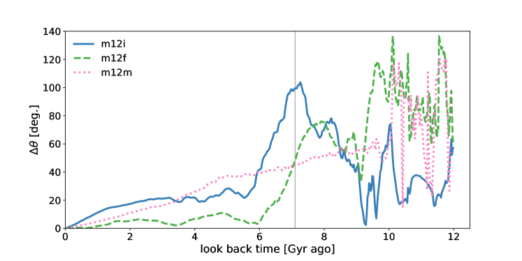
Figure 8: The dynamical histories of the 3 MW-like simulated galaxies in FIRE-2. The angle $\Delta\theta$ of the normal vector of the galaxy disk relative to its present-day direction is plotted versus lookback time. If $\Delta\theta$ changes rapidly, then the evolution of the galaxy is chaotic; if $\Delta\theta$ changes slowly, then the galaxy evolves smoothly. The disk orientations of galaxies m12f and m12m changed rapidly at the beginning and evolved more smoothly after 8 Gyr ago. Galaxy m12i evolved more smoothly than the other two galaxies before 8 Gyr ago, allowing massive satellites that fell into m12i up to 10.3 Gyr ago to remain clustered in action space at $z=0$. A vertical line shows the time boundary for well-recovered satellites-7.1 Gyr ago.

In this work we have demonstrated, using simulation data, that it is possible to find accreted satellites using cluster analysis in action space. We have deliberately focused on a fairly idealized set of circumstances: (a) we assumed that phase space coordinates of all star particles were known with no error; (b) we assumed nearly perfect knowledge of the gravitational potential arising from stars, dark matter and gas (although we approximated the potentials as axisymmetric even though they are triaxial); (c) we had perfect knowlegde of the merger history of the galaxies and therefore the true masses and infall times of the satellites. In future applications of this method to observational data, the following improvements should be explored.

1. As with all cosmological-hydrodynamical simulations, despite being until very recently the highest-resolution such simulations ever conducted of MW-mass halos (Applebaum et al., 2020), resolution limits our results to accreted structures at the stellar mass of classical dwarf galaxies and higher, since each star particle in the FIRE-2 simulations is 7100 ${\rm\,M_{\odot}}$. The total number of accreted star particles used in our analysis is also orders of magnitude smaller than the number of accreted stars with 6D phase space coordinates (from Gaia and future large ground based surveys such as 4MOST (de Jong et al., 2012), WEAVE (Dalton et al., 2014), DESI (DESI Collaboration et al., 2016a, b), which are expected to yield 6 phase space coordinates for 3–4 million stars. The performance of our clustering technique when scaled up by 3–4 orders of magnitude in particle number has yet to be tested. On the other hand, if we restrict ourselves to, e.g., RR Lyrae variables, then the conversion rate between the real data set and the simulation data set is about one star per star particle, and the analysis in this work can be more easily done. In addition, real data have observational errors and for this study we have assumed that all phase space coordinates are known perfectly. Additional studies with more realistic mock datasets like the ananke data set (Sanderson et al., 2020) are needed to assess how well Enlink performs under realistic conditions.

2. It is necessary to find an objective way to determine $N_{\mathrm{min}}$, the parameter used by Enlink  to determine a “reasonable” size for a cluster (Section 3.2). In this study $N_{\mathrm{min}}$  was selected by trial and error in order to ensure that the number of groups that Enlink  produced was close to the number of satellites that were known to have been accreted (as described in Section 2). An objective way to determine $N_{\mathrm{min}}$  and the other parameters that are used in the Enlink  cluster analysis algorithm, is needed to evaluate the quality of clusters found. We found that the conventional silhouette plots (Rousseeuw, 1987) are not useful here, since many satellites are irregularly shaped in the action space and could be incorrectly classified by silhouette values. The choice of parameters for cluster analysis has been largely ignored in previous papers, and should be investigated in future.

3. Stellar metallicities and the abundance of individual elements in a star are also well conserved quantities that contain a substantial amount of information about the host satellite in which the star was born. However the stars in a satellite can have a range of [Fe/H] and $\alpha$-element abundance ratios as well as gradients in the abundances of other elements. Sanderson et al. (2017) show that including the abundance of certain elements (e.g. $N$, $Ca$) can improve the recovery of the Galactic mass model built through cluster analysis. Incorporating metallicities of stars as features into cluster analysis might improve the performance of current results from cluster analysis in action space.

4. The inclusion of metallicities of stars can also help to determine the masses of individual satellites (through the mass-metallicity relationship) and hence action-space clustering can be used to determine the number of accreted satellites per unit mass $N(M)$, a parameter that is a sensitive probe of the model of dark matter.

5. We have assumed in this work that the overall gravitational potential of each galaxy is axisymmetric rather than triaxial. This restriction was driven by the fact that the most efficient action finders available (e.g. AGAMA) are restricted to oblate axisymmetric potentials. Triaxial action finders (Sanders & Binney, 2015a, b) exist but are currently not fast enough to be useful for analysis of large datasets. Development of fast triaxial action finders would be extremely helpful.

Appendix A Classification Tree Method

We use a binary classification tree (Breiman et al., 1984) to objectively determine the boundaries between well-recovered and poorly-recovered satellites in the $T_{\mathrm{infall}}$  - $M_{\mathrm{tot}}$  space and $T_{\mathrm{infall}}$  -$M_{\rm stellar}$ space. A classification tree tries to divide the multi-dimensional space covered by the input data into a series of regions, so that the data points inside each region are as pure (having the same label) as possible. To grow such a classification tree, we do several binary splits based on whether a feature is greater than or equal to ($\geq$) or smaller than ($<$) the split value. The rectangular region before a split is called a parent node, while the two sub-regions resulting from the binary split are called the children nodes. If a node has no children nodes, then it is called a leaf node. The impurity of a node indicates how diverse the labels of data points in a node are, and can be measured by cross-entropy, Gini-index or misclassification error. For details on these scales of impurity, see Hastie et al. (2001). For one parent node with $N_{\rm parent}$ data points and two children nodes with $N_{\rm left}$ and $N_{\rm right}$ data points resulting from a split at one feature $f_{i}=x$, calculate the quality of split $Q(f_{i},x)$:

$$Q(f_{i},x)={\rm Impurity(parent\leavevmode\nobreak\ node)}$$

$$-\frac{N_{\rm left}}{N_{\rm parent}}{\rm Impurity(left\leavevmode\nobreak\ child)}$$

$$-\frac{N_{\rm right}}{N_{\rm parent}}{\rm Impurity(right\leavevmode\nobreak\ child)}$$ (6)

The feature $f_{i}$ and value $x$ that maximize $Q(f_{i},x)$ are the split feature and split value of a binary split. A tree can be grown by adding binary splits in this way until each terminal node is pure and cannot be further split. We then prune the tree by giving a penalty proportional to the size of the tree, until a balance between accuracy and size of tree is reached. Fig. 9 shows the diagram of tree generated from $\log_{10}(M_{\rm tot}/{\rm\,M_{\odot}})$ and $T_{\mathrm{infall}}$ in Gyr ago as input data. In each leaf node, a “well” or “poorly” indicates the prediction on the label of this node by majority vote. A red number in each leaf node is the number of satellites that are not well-recovered in this node, while the blue number corresponds to the number of well-recovered satellites in this node. The tree with $\log_{10}(M_{\rm stellar}/{\rm\,M_{\odot}})$ and $T_{\mathrm{infall}}$ in Gyr ago as input is similar to the tree in Fig. 9, except that the split in $\log_{10}(M_{\rm stellar}/{\rm\,M_{\odot}})$ locates at 6.1.

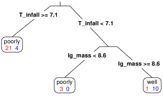
Figure 9: A classification tree used in Section 4.1 to derive the boundaries between well-recovered and poorly-recovered satellites. “T_infall” indicates $T_{\mathrm{infall}}$  in Gyr ago, “lg_mass” represents $\log_{10}(M_{\rm tot}/{\rm\,M_{\odot}})$. A “well” or “poorly” in each leaf node indicates the prediction of the label of data points in this node by majority vote, with “well” corresponding to well-recovered and “poorly” corresponding to poorly-recovered. The red and blue numbers in each leaf node indicate the numbers of poorly-recovered and well-recovered satellites in this leaf node, respectively. The tree with $\log_{10}(M_{\rm stellar}/{\rm\,M_{\odot}})$ and $T_{\mathrm{infall}}$ in Gyr ago as input is similar, except that the split in $\log_{10}(M_{\rm stellar}/{\rm\,M_{\odot}})$ is located at 6.1.

References

- Antoja et al. (2018) Antoja T., et al., 2018, Nature, 561, 360
- Applebaum et al. (2020) Applebaum E., Brooks A. M., Christensen C. R., Munshi F., Quinn T. R., Shen S., Tremmel M., 2020, arXiv e-prints, p. arXiv:2008.11207
- Behroozi et al. (2013a) Behroozi P. S., Wechsler R. H., Wu H.-Y., 2013a, ApJ, 762, 109
- Behroozi et al. (2013b) Behroozi P. S., Wechsler R. H., Wu H.-Y., Busha M. T., Klypin A. A., Primack J. R., 2013b, ApJ, 763, 18
- Bell et al. (2008) Bell E. F., et al., 2008, ApJ, 680, 295
- Belokurov et al. (2018) Belokurov V., Erkal D., Evans N. W., Koposov S. E., Deason A. J., 2018, MNRAS, 478, 611
- Besla et al. (2007) Besla G., Kallivayalil N., Hernquist L., Robertson B., Cox T. J., van der Marel R. P., Alcock C., 2007, ApJ, 668, 949
- Besla et al. (2010) Besla G., Kallivayalil N., Hernquist L., van der Marel R. P., Cox T. J., Kereš D., 2010, ApJ, 721, L97
- Binney & Tremaine (2008) Binney J., Tremaine S., 2008, Galactic Dynamics: Second Edition. Princeton University Press:Princeton, NJ, USA
- Bonaca et al. (2019) Bonaca A., Hogg D. W., Price-Whelan A. M., Conroy C., 2019, ApJ, 880, 38
- Borsato et al. (2020) Borsato N. W., Martell S. L., Simpson J. D., 2020, MNRAS, 492, 1370
- Breiman et al. (1984) Breiman L., Friedman J., Stone C. J., Olshen R. A., 1984, Classification and regression trees. CRC press
- Bullock & Boylan-Kolchin (2017) Bullock J. S., Boylan-Kolchin M., 2017, ARA&A, 55, 343
- Cooper et al. (2010) Cooper A. P., et al., 2010, MNRAS, 406, 744
- DESI Collaboration et al. (2016a) DESI Collaboration et al., 2016a, ArXiv e-prints, arXiv:1611.00036,
- DESI Collaboration et al. (2016b) DESI Collaboration et al., 2016b, ArXiv e-prints, arXiv:1611.00037,
- Dalton et al. (2014) Dalton G., et al., 2014, Project overview and update on WEAVE: the next generation wide-field spectroscopy facility for the William Herschel Telescope. SPIE, p. 91470L, doi:10.1117/12.2055132
- Erkal et al. (2016) Erkal D., Belokurov V., Bovy J., Sanders J. L., 2016, Monthly Notices of the Royal Astronomical Society, 463, 102
- Evans et al. (2018) Evans D. W., et al., 2018, A&A, 616, A4
- Fabricius et al. (2016) Fabricius C., et al., 2016, A&A, 595, A3
- Fakhouri & Ma (2008) Fakhouri O., Ma C.-P., 2008, MNRAS, 386, 577
- Feldmann & Spolyar (2015) Feldmann R., Spolyar D., 2015, MNRAS, 446, 1000
- Font et al. (2011) Font A. S., McCarthy I. G., Crain R. A., Theuns T., Schaye J., Wiersma R. P. C., Dalla Vecchia C., 2011, MNRAS, 416, 2802
- Garrison-Kimmel et al. (2018) Garrison-Kimmel S., et al., 2018, MNRAS, 481, 4133
- Garrison-Kimmel et al. (2019) Garrison-Kimmel S., et al., 2019, Monthly Notices of the Royal Astronomical Society, 487, 1380
- Gómez et al. (2010) Gómez F. A., Helmi A., Brown A. G. A., Li Y.-S., 2010, MNRAS, 408, 935
- Gudin et al. (2021) Gudin D., et al., 2021, ApJ, 908, 79
- Harding et al. (2001) Harding P., Morrison H. L., Olszewski E. W., Arabadjis J., Mateo M., Dohm-Palmer R. C., Freeman K. C., Norris J. E., 2001, AJ, 122, 1397
- Harmsen et al. (2017) Harmsen B., Monachesi A., Bell E. F., de Jong R. S., Bailin J., Radburn-Smith D. J., Holwerda B. W., 2017, MNRAS, 466, 1491
- Hastie et al. (2001) Hastie T., Tibshirani R., Friedman J., 2001, The Elements of Statistical Learning. Springer Series in Statistics, Springer New York Inc., New York, NY, USA
- Helmi & de Zeeuw (2000) Helmi A., de Zeeuw P. T., 2000, MNRAS, 319, 657
- Helmi et al. (2018) Helmi A., Babusiaux C., Koppelman H. H., Massari D., Veljanoski J., Brown A. G. A., 2018, Nature, 563, 85
- Hopkins (2015) Hopkins P. F., 2015, MNRAS, 450, 53
- Hopkins et al. (2018) Hopkins P. F., et al., 2018, Monthly Notices of the Royal Astronomical Society, 480, 800
- Johnston et al. (1996) Johnston K. V., Hernquist L., Bolte M., 1996, ApJ, 465, 278
- Lazar et al. (2020) Lazar A., et al., 2020, MNRAS, 497, 2393
- Limberg et al. (2021) Limberg G., et al., 2021, ApJ, 907, 10
- Lindegren et al. (2016) Lindegren L., et al., 2016, A&A, 595, A4
- Lindegren et al. (2018) Lindegren L., et al., 2018, A&A, 616, A2
- Lynden-Bell & Lynden-Bell (1995) Lynden-Bell D., Lynden-Bell R. M., 1995, Mon. Not. Roy. Astron. Soc., 275, 429
- Monachesi et al. (2019) Monachesi A., et al., 2019, MNRAS, 485, 2589
- Myeong et al. (2018a) Myeong G. C., Evans N. W., Belokurov V., Sanders J. L., Koposov S. E., 2018a, Monthly Notices of the Royal Astronomical Society, 478, 5449
- Myeong et al. (2018b) Myeong G. C., Evans N. W., Belokurov V., Sand ers J. L., Koposov S. E., 2018b, ApJ, 856, L26
- Myeong et al. (2019) Myeong G. C., Vasiliev E., Iorio G., Evans N. W., Belokurov V., 2019, MNRAS, 488, 1235
- Naidu et al. (2020) Naidu R. P., Conroy C., Bonaca A., Johnson B. D., Ting Y.-S., Caldwell N., Zaritsky D., Cargile P. A., 2020, arXiv e-prints, p. arXiv:2006.08625
- Necib et al. (2019) Necib L., Ostdiek B., Lisanti M., Cohen T., Freytsis M., Garrison-Kimmel S., 2019, arXiv e-prints, p. arXiv:1907.07681
- Necib et al. (2020) Necib L., et al., 2020, Nature Astronomy,
- Ostdiek et al. (2020) Ostdiek B., et al., 2020, Astron. Astrophys., 636, A75
- Panithanpaisal et al. (2021) Panithanpaisal N., Sanderson R. E., Wetzel A., Cunningham E. C., Bailin J., Faucher-Giguère C.-A., 2021, arXiv e-prints, p. arXiv:2104.09660
- Perryman et al. (2001) Perryman M. A. C., et al., 2001, A&A, 369, 339
- Pillepich et al. (2015) Pillepich A., Madau P., Mayer L., 2015, ApJ, 799, 184
- Price-Whelan & Bonaca (2018) Price-Whelan A. M., Bonaca A., 2018, ApJ, 863, L20
- Roederer et al. (2018) Roederer I. U., Hattori K., Valluri M., 2018, AJ, 156, 179
- Rousseeuw (1987) Rousseeuw P. J., 1987, Journal of Computational and Applied Mathematics, 20, 53
- Samuel et al. (2020a) Samuel J., Wetzel A., Chapman S., Tollerud E., Hopkins P. F., Boylan-Kolchin M., Bailin J., Faucher-Giguère C.-A., 2020a, arXiv e-prints, p. arXiv:2010.08571
- Samuel et al. (2020b) Samuel J., et al., 2020b, MNRAS, 491, 1471
- Sanders & Binney (2015a) Sanders J. L., Binney J., 2015a, TACT: The Action Computation Tool (ascl:1512.020)
- Sanders & Binney (2015b) Sanders J. L., Binney J., 2015b, MNRAS, 447, 2479
- Sanderson et al. (2017) Sanderson R., Wetzel A., Sharma S., Hopkins P., 2017, Galaxies, 5, 43
- Sanderson et al. (2020) Sanderson R. E., et al., 2020, ApJS, 246, 6
- Santistevan et al. (2020) Santistevan I. B., Wetzel A., El-Badry K., Bland-Hawthorn J., Boylan-Kolchin M., Bailin J., Faucher-Giguère C.-A., Benincasa S., 2020, MNRAS, 497, 747
- Santistevan et al. (2021) Santistevan I. B., Wetzel A., Sanderson R. E., El-Badry K., Samuel J., Faucher-Giguère C.-A., 2021, arXiv e-prints, p. arXiv:2102.03369
- Sharma & Johnston (2009) Sharma S., Johnston K. V., 2009, The Astrophysical Journal, 703, 1061
- Tissera et al. (2013) Tissera P. B., Scannapieco C., Beers T. C., Carollo D., 2013, MNRAS, 432, 3391
- Tremaine (1999) Tremaine S., 1999, MNRAS, 307, 877
- Vasiliev (2018) Vasiliev E., 2018, Monthly Notices of the Royal Astronomical Society, 482, 1525
- Wetzel & Garrison-Kimmel (2020a) Wetzel A., Garrison-Kimmel S., 2020a, HaloAnalysis: Read and analyze halo catalogs and merger trees (ascl:2002.014)
- Wetzel & Garrison-Kimmel (2020b) Wetzel A., Garrison-Kimmel S., 2020b, GizmoAnalysis: Read and analyze Gizmo simulations (ascl:2002.015)
- Wetzel et al. (2016) Wetzel A. R., Hopkins P. F., hoon Kim J., Faucher-Giguère C.-A., Kereš D., Quataert E., 2016, The Astrophysical Journal, 827, L23
- Widrow et al. (2012) Widrow L. M., Gardner S., Yanny B., Dodelson S., Chen H.-Y., 2012, ApJ, 750, L41
- Yu et al. (2020) Yu S., et al., 2020, MNRAS, 494, 1539
- Yuan et al. (2020) Yuan Z., et al., 2020, ApJ, 891, 39
- Zavala & Frenk (2019) Zavala J., Frenk C. S., 2019, Galaxies, 7, 81
- Zolotov et al. (2009) Zolotov A., Willman B., Brooks A. M., Governato F., Brook C. B., Hogg D. W., Quinn T., Stinson G., 2009, ApJ, 702, 1058
- Zolotov et al. (2012) Zolotov A., et al., 2012, ApJ, 761, 71
- de Jong et al. (2012) de Jong R. S., et al., 2012, in McLean I. S., Ramsay S. K., Takami H., eds, Society of Photo-Optical Instrumentation Engineers (SPIE) Conference Series Vol. 8446, Ground-based and Airborne Instrumentation for Astronomy IV. SPIE, pp 252 – 266, doi:10.1117/12.926239, https://doi.org/10.1117/12.926239