On the Use of Field RR Lyrae as Galactic Probes. III. The $\alpha$-element abundances

Abstract

We provide the largest and most homogeneous sample of $\alpha$-element (Mg, Ca, Ti) and iron abundances for field RR Lyrae (RRLs, 162 variables) by using high-resolution spectra. The current measurements were complemented with similar abundances available in the literature for 46 field RRLs brought to our metallicity scale. We ended up with a sample of old (t$\geq$ 10 Gyr), low-mass stellar tracers (208 RRLs: 169 fundamental, 38 first overtone, 1 mixed mode) covering three dex in iron abundance (-3.00$\leq$[Fe/H]$\leq$0.24). We found that field RRLs are $\sim$0.3 dex more $\alpha$-poor than typical Halo tracers in the metal-rich regime, ([Fe/H]$\geq$-1.2) while in the metal-poor regime ([Fe/H]$\leq$-2.2) they seem to be on average $\sim$0.1 dex more $\alpha$-enhanced. This is the first time that the depletion in $\alpha$-elements for solar iron abundances is detected on the basis of a large, homogeneous and coeval sample of old stellar tracers. Interestingly, we also detected a close similarity in the [$\alpha$/Fe] trend between $\alpha$-poor, metal-rich RRLs and red giants (RGs) in the Sagittarius dwarf galaxy as well as between $\alpha$-enhanced, metal-poor RRLs and RGs in ultra faint dwarf galaxies. These results are supported by similar elemental abundances for 46 field Horizontal Branch (HB) stars. These stars share with RRLs the same evolutionary phase and the same progenitors. This evidence further supports the key role that old stellar tracers play in constraining the early chemical enrichment of the Halo and, in particular, in investigating the impact that dwarf galaxies have had in the mass assembly of the Galaxy.

1 Introduction

The chemical abundances of stellar atmospheres preserve the signature of the molecular clouds that formed them. While some of their elements can be altered during stellar evolution, such as the LiCNO group and (rarely) some neutron-capture elements, stellar atmospheres remain the ideal subjects of Galactic archeology. Different chemical species are formed by processes with their own mass and time scales and, coupled with the age of the stellar tracers of interest, reveal the chemical enrichment history of different components of the Galaxy.

The even-Z light elements that are multiples of He nuclei are called $\alpha$-elements. In the past, it was believed that they were created by the successive capture of He nuclei. However, it is now understood that, while several elements are commonly grouped under the banner of $\alpha$-elements, not all of them are created equally nor are all of them equally easy to measure (Woosley & Weaver, 1995; McWilliam, 2016; Curtis et al., 2019). In particular the noble gasses Ne and Ar cannot be detected, and S is rarely measured in optical spectra (Gratton et al., 2004). A similar limitation applies to O, indeed O abundances are typically based either on two weak OI forbidden lines (6300, 6363 Å) or on OI triplet lines (7774, 9263 Å) that are affected by temperature uncertainties and by non-LTE effects (McWilliam, 1997). Like oxygen, the much easier to measure Mg is created in the hydrostatic evolution of massive stars and released on supernovae type II (SNe II) events.

It is affected by the reaction mechanisms known as the ”p-process” (Wallerstein et al., 1997), i.e., the production of proton-rich nuclei by a proton-capture mechanism. The other three species with easily detectable lines are Si, Ca and Ti. Of these, the first two are likely mainly produced during SNe II events, being thus considered ”explosive” $\alpha$-elements. The third, Ti, has a vast number of absorption lines that can be detected on a broad wavelength and metallicity range. It is sometimes considered as an iron-peak element (Timmes et al., 1995) with possibly multiple formation channels. Indeed, its dominant isotope is actually ${}^{\text{48}}_{\text{22}}$Ti, which is not a multiple of an $\alpha$ particle. Yet the trend of titanium with metallicity follows quite well those of other $\alpha$-elements, and suggests that, regardless of the precise formation channels, these chemical species are formed at similar rates in similar astrophysical sites.

Stellar evolution models point to SNe Ia as the result of the thermonuclear explosions triggered by the binary interaction between an accreting white dwarf and its companion. The presence of a white dwarf implies a time scale of the order of billions of years. The yields of such explosions carry mostly iron, and so an environment enriched mostly by SNe Ia would have a decreasing [$\alpha$/Fe] ratio as iron abundance increases. Indeed, in the [$\alpha$/Fe] versus [Fe/H] plane, this decrease is commonly called the ”knee”, and is associated with the metallicity at which the SNe Ia began to dominate the enrichment of the interstellar medium (e.g., Matteucci & Brocato, 1990).

The main producers of $\alpha$-elements, however, are the SNe II. They are the result of the core-collapse of massive stars ($\gtrsim$8 M_⊙), with a time scale of the order of one to ten million years. They enrich the interstellar medium with both iron and $\alpha$-elements, with the yields of the latter increasing as the mass of the SNe II progenitor increases (Kobayashi et al., 2006). This means that the slope of the [$\alpha$/Fe] abundance ratio and, in particular, its spread at fixed iron content can provide firm constraints on the variation of the initial mass Function (IMF) as a function of both time and environment (McWilliam et al., 2013; Hendricks et al., 2014a; Lemasle et al., 2014; Reichert et al., 2020).

Thus, the fine structure of the [$\alpha$/Fe] abundance ratio as a function of iron abundance has been in the intersection of several theoretical and empirical investigations (Matteucci & Greggio, 1986). For over forty years, $\alpha$-elements have been known to be enhanced in primarily old and metal-poor populations such as field Halo stars and globular clusters (GCs) (Wallerstein et al., 1963; Sneden et al., 1979; Cohen, 1981; Pilachowski et al., 1983; McWilliam, 1997; Venn et al., 2004; Pritzl et al., 2005; Carretta et al., 2009a). The current evidence is suggesting a steady decrease in the [$\alpha$/Fe] abundance ratio for iron abundances more metal-rich than [Fe/H]$\approx$-0.7. However, the number of truly old, metal-rich stellar tracers is quite limited (see Figs. 10 and 11 in Gonzalez et al., 2011). Indeed, it is not clear yet whether old stellar tracers display the same slope in the [$\alpha$/Fe] versus [Fe/H] plane as intermediate and young disk stellar populations in approaching solar iron abundance.

Two major concerns are involved in the selection of the stellar sample to be employed in the investigation of the chemical enrichment history of the Halo. First, although the [$\alpha$/Fe] abundance ratio is a solid diagnostic, stars covering a broad range in iron abundances with homogeneous and accurate estimates are necessary. Second, any discussion of chemical enrichment history must necessarily take into account the age of the stellar tracers that are being employed. Individual age estimates for field stars require very precise reddening and distance measurements, and therefore samples of field stars suffer various degrees of contamination. For field RGs this limitation becomes even more severe because they originate from progenitors that cover a broad range in mass. The natural targets for age-related experiments are GCs because they have accurate individual age estimates provided by isochrone fitting (e.g. Salaris & Weiss, 1998; VandenBerg et al., 2013). However, the current spectroscopic investigations that are focused on GCs include only a few metal-rich systems (Pritzl et al., 2005; Carretta et al., 2009a, b, 2010a; Gonzalez et al., 2011).

These two concerns can be addressed at once with the use of field RR Lyrae variable stars. RRLs are solid tracers of old stellar populations, well known to be evolved low mass stars with ages necessarily greater than 10 Gyr (Walker et al., 2019; Savino et al., 2020). They can be identified by the shape, period, and amplitude of their photometric light curves, all of which are reddening- and distance-independent. Their classification, coupled with with spectroscopic atmospheric parameters, provides a strongly univocal identification and make any sample contamination extremely unlikely. The RRLs also are known to cover a broad range in metallicity (Wallerstein et al., 2012; Chadid et al., 2017; Sneden et al., 2017; Crestani et al., 2021) and far outnumber GCs. Indeed, while only roughly 180 GCs have been identified in the Galaxy (Harris, 1996, 2010), the number of field RRLs thanks to long term photometric surveys and to Gaia is at least a thousand times larger. This means that the RRLs can trace the variation of chemical abundances across the Galactic spheroid with very high spatial resolution. The variation in stellar mass of RRLs is at most of the order of 30-40%, i.e. from $\approx$0.60 to $\approx$0.85 $M_{\odot}$, therefore, they are only minimally affected by the shape of the IMF. Moreover, the RRLs are also minimally affected by the time dependence, because they formed on a time interval of the order of two Gyr.

In the current work, we aim to investigate the impact that stellar age has on the [$\alpha$/Fe] vs [Fe/H] plane using high resolution, high signal-to-noise ratio (SNR) spectra of 162 field RRLs. Among them, 138 are fundamental mode pulsators (RRab), 23 first overtone pulsators (RRc), and one mixed mode pulsator (RRd). This data set is described in Sect. 2. The current homogeneous measurements of $\alpha$-element and iron abundances were complemented with similar measurements for field RRLs and HB stars available in the literature and brought to our scale, as described in Sect. 3. In Sect. 4 we address how the atmospheric parameters and chemical abundances were computed. Results are shown and discussed in Sect. 5. In Sect. 6, we summarize this investigation and briefly outline future perspectives.

2 Spectroscopic data set

We collected a sample of 407 high resolution spectra for 162 field RRLs (138 RRab, 23 RRc, 1 RRd). In order to obtain a high enough SNR ($\gtrapprox$ 50 per pixel) for chemical abundance analysis, we stacked low SNR spectra of the same star acquired at the same phase and with the same spectrograph, as described in more detail further below. This process resulted in 243 spectra that were analysed individually.Among them, 51 were acquired with the echelle spectrograph at du Pont (Las Campanas Observatory), 74 with UVES (Dekker et al., 2000) and 16 with X-shooter (Vernet et al., 2011) at VLT (ESO, Cerro Paranal Observatory), 18 with HARPS (Mayor et al., 2003) at the 3.6m telescope and two with FEROS (Kaufer et al., 1999) at the 2.2m MPG telescope (ESO, La Silla Observatory), five with HARPS-N (Cosentino et al., 2012) at the Telescopio Nazionale Galileo (Roque de Los Muchachos Observatory), 47 with HRS (Crause et al., 2014) at SALT (South African Astronomical Observatory), 28 with the HDS (Noguchi et al., 2002) at Subaru (National Astronomical Observatory of Japan), and two with the echelle spectrograph (Weber et al., 2012) at STELLA (Izaña Observatory).

Representative spectra for each of these spectrographs are shown in Fig. 1. Their typical wavelength ranges, resolutions and SNR are listed in Tab. 1.

Table 1: Typical characteristics of each instrument used in this work.

Spectrograph	Telescope	Wavelength	Resolution	SNR
		Range
		(Å)
echelle	du Pont	3700 – 9100	27,000	70
UVES	VLT	3000 – 6800	35,000 – 107,000	76
X-shooter	VLT	3000 –10200	18,400	86
HARPS	3.6m	3700 – 6900	80,000 – 115,000	45
FEROS	2.2m MPG	3500 – 9200	48,000	53
HARPS-N	TNG	3900 – 6900	115,000	65
HRS	SALT	3900 – 8800	40,000	61
HDS	Subaru	5060 – 7840	60,000	95
echelle	STELLA	3860 – 8820	55,000	74

Note. — The wavelength ranges and resolutions are approximate. Different instrumental configurations result in different values, including wavelength coverage gaps. The archival data for UVES displayed a significant variety of configurations. Only the most representative values are shown.

Continuum normalization and Doppler-shift corrections were made using the National Optical Astronomy Observatory libraries for IRAF (Image Reduction and Analysis Facility, Tody, 1993). Further information about the sample selection and radial velocity studies for the spectra analysed in this work can be found in Fabrizio et al. (2019); Bono et al. (2020), and Crestani et al. (2021).

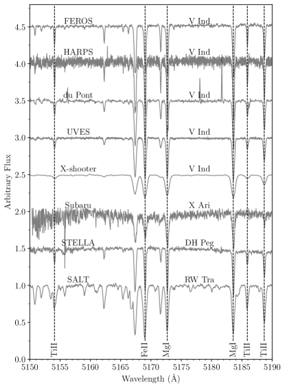
Figure 1: Representative high resolution spectra for all spectrographs used in this work. The top five spectra are of V Ind ([Fe/H] = -1.63$\pm$± 0.03, RRab) at the same pulsation phase. They are followed by random phase spectra for X Ari ([Fe/H] = -2.59$\pm$0.05, RRab), DH Peg ([Fe/H] = -1.37$\pm$0.05, RRc), and RW Tra ([Fe/H] = 0.13$\pm$0.06, RRab). The dashed lines indicate the iron and $\alpha$-element absorption lines in this wavelength region.

The stacking of spectra was performed after these steps. We made an initial selection based on phase, followed by a visual inspection. This ensured that all the spectra to be stacked displayed similar line depths and introduced no artifacts in the final stacked spectrum. Of the 243 final spectra that we analysed, 178 were collected with high SNR and did not require stacking, 26 were the result of the stacking of two spectra, and 39 of three to seven spectra.

3 Spectroscopic samples

The 162 RRLs described above form the This Work (TW-RRL) sample. Previous high resolution metallicity measurements are available in the literature for 47 of these stars. They were used to transform iron and $\alpha$-element abundances into a homogeneous abundance scale. This supplied us with 69 measurements for 46 stars made by nine previous works. Note that the measurements taken from For & Sneden (2010); For et al. (2011); Chadid et al. (2017) and Sneden et al. (2017) are natively in our scale and require no shifts. Indeed, a comparison between 23 RRLs measured both in those works and in the present work resulted in absolute differences smaller than 0.10 dex for all abundances. Note that the investigation from For & Sneden (2010) was focused on non-variable HB stars for which we did not perform a reanalysis, but they used the same line list, instrument, and methodology as For et al. (2011). Once all abundances of interest were brought to our scale, multiple measurements for the same star were averaged. This allowed us to form the Literature RRL (Lit-RRL) sample, with 46 stars. We will refer to the TW-RRL and Lit-RRL samples together as the RRL sample. Its basic characteristics are shown in Tab. 2. The individual measurements for the literature stars both in their native scale and in our scale are shown in Tab. 3, alongside their references.

Table 2: Basic information of the entire RRL sample.

GaiaID	Star	RAJ2000	DecJ2000	Vmag	Vamp	P	Class	Sample
(DR2)		(deg)	(deg)	(mag)	(mag)	(day)
4224859720193721856	AA Aql	309.5628	-2.8903	11.831	1.275	0.3618	RRab	TW-RRL
2608819623000543744	AA Aqr	339.0161	-10.0153	12.923	1.087	0.6089	RRab	TW-RRL
3111925220109675136	AA CMi	109.3299	1.7278	11.558	0.965	0.4763	RRab	TW-RRL
1234729400256865664	AE Boo	221.8968	16.8453	10.651	0.423	0.3149	RRc	TW-RRL
2150632997196029824	AE Dra	276.7780	55.4925	12.474	0.799	0.6027	RRab	Lit-RRL

Note. — Identification, coordinates, average visual magnitude (Vmag), visual amplitude (Vamp), period (P), classification, and sample of the RRL stars. Table 2 is published in its entirety in machine-readable format. A portion is shown here for guidance regarding its form and content.

Table 3: RRL abundances adopted from the literature.

GaiaID	[Fe/H]${}_{\text{o}}$	[Mg/Fe]${}_{\text{o}}$	[Ca/Fe]${}_{\text{o}}$	[Ti/Fe]${}_{\text{o}}$	[Fe/H]	[Mg/Fe]	[Ca/Fe]	[Ti/Fe]	Reference
(DR2)
15489408711727488	-2.59		0.34	0.43	-2.59		0.34	0.43	C17
15489408711727488	-2.48	0.48	0.45	0.43	-2.68	0.61	0.44	0.38	C95
15489408711727488	-2.47		0.29		-2.48		0.39		L96
15489408711727488	-2.19	0.48	0.29	0.80	-2.42	0.36	0.32	0.91	P15
234108363683247616	-0.28		0.14		-0.28		0.09		F96

Note. — Identification, iron and $\alpha$-element abundances in both their original (subscript o) scale and in our scale for the Lit-RRL sample. Table 3 is published in its entirety in machine-readable format. A portion is shown here for guidance regarding its form and content. References and number of stars in common with the TW-RRL sample are: C17, 13: Chadid et al. (2017); C95, 8: Clementini et al. (1995); F10, 1: For & Sneden (2010); F11, 5: For et al. (2011); F96, 4: Fernley & Barnes (1996), G14, 2: Govea et al. (2014); L96, 8: Lambert et al. (1996); P15, 8: Pancino et al. (2015); S17, 5: Sneden et al. (2017).

For & Sneden (2010) investigated the chemical abundances of metal-poor field red HB stars, in our same metallicity and $\alpha$-element scale. We found that two of their stars were later classified as RRL. One of them is already in the TW-Lit sample, and the other was added to the Lit-RRL sample. We adopted the data for the remaining HB stars as the Lit-HB sample, with 46 stars. The complete sample of RRL and HB stars in this work will be referred to as the RRL+HB sample.

4 Chemical abundance measurements

We have applied the same iron line list and LTE line analysis described in Crestani et al. (2021). In brief, equivalent widths were measured manually with the splot IRAF. We only considered lines with equivalent widths between 15 and 150 mÅ in order to avoid spurious measurements and saturated lines. We derived the effective temperature (T${}_{\text{eff}}$), surface gravity (log(g)), microturbulent velocity ($\xi_{\text{t}}$), and metallicity ([Fe/H]) for each atmosphere using the equivalent widths of the neutral and single-ionized iron lines. For this, we followed the method of iteratively changing the atmospheric parameters in order to achieve excitation equilibrium of FeI lines (T${}_{\text{eff}}$), ionization equilibrium between FeI and FeII lines (log(g)), and no trend between the abundance of each individual FeI line against its respective reduced equivalent width ($\xi_{\text{t}}$). This process was done using the 2019 release of Moog (Sneden, 1973), the Moog wrapper pyMOOGi developed by M. Adamow, and an interpolated grid of $\alpha$-enhanced ([$\alpha$/Fe] = 0.4 dex)ATLAS9 model atmospheres (Castelli & Kurucz, 2003). The adopted atmospheric values for each individual measurement are shown in Tab. 4.

Once the final model atmosphere was constrained, the abundances of the $\alpha$-elements were computed from the equivalent widths of their lines. The line list is shown in Tab. 5, alongside the reference for their excitation potential (EP) and oscillator strength (log(gf)). As with iron, only lines with equivalent widths between 15 and 150 mÅ were considered. Solar abundance values were adopted from Asplund et al. (2009). In the case where more than one line was available for a given chemical species, the median value was adopted.

A single RRL can undergo changes as large as 1000 K in effective temperature and 1 dex in log(g) (For et al., 2011). Thus, the robustness of a given method of abundance determination can be assessed by its capacity to recover coherent values across the pulsation phase. Similarly, the difference between repeated measurements is a reliable determination of the uncertainty of the measurements. With this in mind, we computed the uncertainties for iron and individual $\alpha$-elements by taking the median absolute deviation between multiple measurements for the same star both in the TW-RRL and Lit-RRL samples. For the TW-RRL sample, this allowed us to determine the typical uncertainty of each chemical species in each spectrograph, which we adopted for the stars with a single measurement. For stars with a single measurement in the Lit-RRL sample, we adopted a fixed uncertainty of 0.10 dex for iron, and 0.15 for each $\alpha$-element. We averaged the abundances of TiI and TiII in order to derive a total [Ti/Fe] ratio. The [TiI/Fe] and [TiII/Fe] are on average shifted by 0.05 dex in our data. Any disagreements between TiI and TiII abundances are reflected in the uncertainties for each star.

To compute the total [$\alpha$/H] abundance, we took the median of [Mg/H], [Ca/H], [TiI/H], and [TiII/H] according to their availability and weighted by their uncertainties. The median absolute deviation between the different $\alpha$-elements was adopted as the uncertainty in the total [$\alpha$/H] abundance. Finally, we subtracted the iron abundance from [$\alpha$/H] for each individual star to arrive at the final [$\alpha$/Fe] value.

4.1 Verification of the T${}_{\text{eff}}$ scale

The atmospheric parameter that most strongly affects the determination of chemical abundances is the effective temperature. As described above, it is essential that the methodology employed for chemical abundance analysis be capable of recovering coherent abundances across the pulsation cycle, i.e. at different values of T${}_{\text{eff}}$. It is already known that spectroscopic studies of RRL in both low and high resolution can achieve excellent precision at random phases (e.g. For et al., 2011; Crestani et al., 2021).

In order to have a sanity check indepedent of spectroscopy, we applied the photometric T${}_{\text{eff}}$ calibration of Alonso et al. (1999, 2001) to a subsample of RRL with V- and K-band photometry. The V-K color was chosen because it is the least affected by uncertainties in the temperature and provides very stable results (Cacciari et al., 2000; Bono, 2003). Photometric T${}_{\text{eff}}$ relations have a limited applicability to the RRLs because these stars cover a wide range of metallicities and moderately high temperatures (see e.g. Table 1 in Alonso et al., 1999). As the RRL are variable stars with continuously changing colors, the application of these calibrations requires either simultaneous or well sampled light curves in both optical and near-infrared bands. Moreover, the phasing itself requires very good determinations of both period and reference epoch. An added difficulty is that, in order to adopt photometric temperatures in a chemical abundance analysis, both photometric and spectroscopic data must be acquired for the same phase. Unfortunately, obtaining all the necessary data for these paired observations is not trivial.

Fortunately enough, we found well sampled V-K colors curves for three variables with a total of seven spectra in the TW-RRL sample: DH Peg (RRc, [Fe/H] = -1.36, two spectra), VY Ser (RRab, [Fe/H] = -1.96, three spectra), and W Tuc (RRab, [Fe/H] = -1.90, two spectra). The photometry was taken from Jones et al. (1988); Barnes et al. (1988); Liu & Janes (1989); Clementini et al. (1990); Fernley et al. (1990); Cacciari et al. (1992). We found a very good agreement between photometric and spectroscopic estimates, with residuals displaying a median $\eta$=39$\pm$47 K, and median absolute deviation $\sigma$=124 K (Fig. 2).

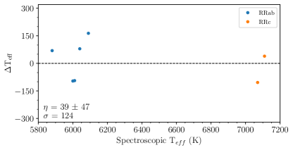
Figure 2: Difference between the photometric and spectroscopic effective temperatures $\Delta$T${}_{\text{eff}}$ for seven measurements of three RRLs. The median ($\eta$) and median absolute deviation ($\sigma$) of the difference is shown on the lower left. See text for details.

Table 4: Atmospheric parameters derived in this work for each individual measurement.

GaiaID	Spectrograph	T${}_{\text{eff}}$	log(g)	$\xi_{\text{t}}$	[FeI/H]	N${}_{\text{FeI}}$	[FeII/H]	N${}_{\text{FeII}}$	N${}_{\text{stack}}$
(DR2)		(K)	(dex)	(km s-1)	(dex)		(dex)
4224859720193721856	SALT	6610$\pm$130	2.70$\pm$0.12	2.52$\pm$0.08	-0.34$\pm$0.24	206	-0.34$\pm$0.22	39	1
4224859720193721856	Subaru	6470$\pm$110	2.62$\pm$0.10	2.42$\pm$0.08	-0.49$\pm$0.17	137	-0.49$\pm$0.16	22	1
2608819623000543744	UVES	5840$\pm$160	1.52$\pm$0.06	3.51$\pm$0.25	-2.31$\pm$0.10	37	-2.31$\pm$0.12	13	1
3111925220109675136	SALT	7090$\pm$180	3.01$\pm$0.15	3.04$\pm$0.16	0.24$\pm$0.24	146	0.24$\pm$0.21	19	1
1234729400256865664	HARPS	6630$\pm$150	2.04$\pm$0.08	2.79$\pm$0.09	-1.62$\pm$0.14	64	-1.62$\pm$0.10	25	2

Note. — Atmospheric parameters for each indvidual measurement of the TW-RRL sample. The columns N${}_{\text{FeI}}$ and N${}_{\text{FeII}}$ contain the number of adopted FeI and FeII lines, respectively. Column N${}_{\text{stack}}$ shows the number of individual exposures that are stacked in order to obtain the measurement. See text for details. Table 4 is published in its entirety in machine-readable format. A portion is shown here for guidance regarding its form and content.

Table 5: List of $\alpha$-element transitions adopted in this work.

Wavelength	Species	EP	log(gf)	Reference
(Å)		(eV)	(dex)
3829.36	12.0	2.709	-0.227	NIST
4571.10	12.0	0.000	-5.620	NIST
4702.99	12.0	4.346	-0.440	NIST
5172.68	12.0	2.712	-0.393	NIST
5183.60	12.0	2.717	-0.167	NIST

Note. — Table 5 is published in its entirety in machine-readable format. A portion is shown here for guidance regarding its form and content. References – NIST: https://www.nist.gov/, LAW2013: Lawler et al. (2013), WOO2013: Wood et al. (2013).

4.2 Validation of the $\alpha$-element abundance scale

The validation of our metallicity scale was performed in Crestani et al. (2021). For the validation of our $\alpha$-element abundance scale, we performed three tests. First, we analysed one high SNR ($\approx$ 350), high dispersion (R=115000) spectrum for Arcturus collected with HARPS. We found the atmospheric parameters T${}_{\text{eff}}$ = 4350$\pm$60 K, log(g) = 1.65$\pm$0.07, $\xi_{\text{t}}$ = 1.75$\pm$0.04 kms^-1, and chemical abundances [FeI/H] = -0.52$\pm$0.06, [FeII/H] = -0.52$\pm$0.20, [Ca/Fe] = 0.08$\pm$0.14, [TiI/Fe] = 0.32$\pm$0.20, and [TiII/Fe] = 0.33$\pm$0.09 dex. These results are in excellent agreement with Ramírez & Allende Prieto (2011). Indeed, the difference in the abundances is 0.00, 0.03, -0.05, -0.12 for Fe, Ca, TiI, and TiII, respectively. Unfortunately, the Mg lines in our line list, optimized for hotter stars, were all saturated in the much colder atmosphere of Arcturus. Second, we performed the same analysis on six red HB stars investigated by Afsar et al. (2018). These stars are only slightly colder than the RRL. The results are shown in Fig. 3, and once again they agree quite well with literature estimates. Third, we made a comparison using directly the equivalent widths of iron and $\alpha$-element for several pairs of stars at similar effective temperature. The analysis of these paired spectra is discussed in Appendix A.

We verified that NLTE corrections do not change the conclusions of our investigation (Sect. 5). As most works in the literature do not make use of such corrections, we opted to not apply them in order to better compare our results to previous ones. Ca, TiI, and TiII display a few lines that appear in all metallicity regimes and allowed us to verify that the averages for each species are not affected by systematics between lines. For Mg, no individual line is measurable in the entire metallicity range, but different lines have superposed metallicity regimes, e.g. one line appears in stars from metal-poor to -intermediate, and another from metal-intermediate to -rich. These considered together exhibit a coherent trend with each other, and with both Ca and Ti. We refer the reader to Appendix B for a detailed discussion of both the NLTE corrections and the behavior of individual lines.

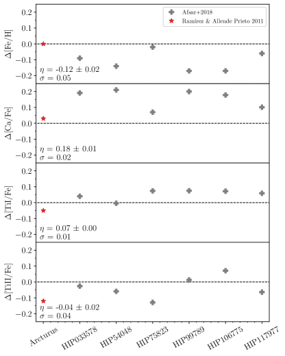
Figure 3: Difference between the iron and $\alpha$-element abundances derived in this work and those of Afsar et al. (2018) for a sample of six HB stars, shown as grey crosses. The median ($\eta$) and median absolute deviation ($\sigma$) of the difference is shown in each panel. A red star shows the same difference for Arcturus (Ramírez & Allende Prieto, 2011).

5 Results and discussion

5.1 The individual species

The final metallicity, individual $\alpha$-element abundance, and total [$\alpha$/Fe] abundance for each RRL and HB star is shown in Tab. 6. The coverage in pulsational amplitude and period of the full RRL sample is shown in the top panels of Fig. 4. The bottom panel of the same figure shows the same sample, but color-coded according to metallicity (see the color bar on the right side).

Fundamental RRLs located in the high-amplitude, short-period (P $\lesssim$ 0.48 day) region, i.e. the so-called HASP region, are confirmed to be more metal-rich than -1.5 dex, as expected from low resolution spectra and globular cluster metallicities (see Fiorentino et al., 2015, 2017). The precision of the current iron abundances strenghtens the evidence that the HASPs trace quite well the transition from fundamental to first overtone RRLs. The RRc seems to show a similar trend: their metal-rich tail is traced by short period variables (P$\leq$0.27 day), although their luminosity amplitudes have typical RRc values. However, the number of metal-rich RRc variables is still too limited to constrain their pulsation properties close to the blue (hot) edge of the RRL instability strip.

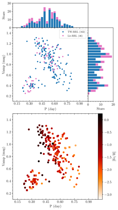
Figure 4: Top: Bailey diagram for the TW-RRL sample (blue), and the Lit-RRL sample (pink). The top and left histograms show the distribution of period and V-band amplitudes, respectively. Bottom: Bailey diagram colored by metallicity according to the color bar on the right. The TW-RRL and the Lit-RRL stars are marked with circles and squares, respectively.

The [X/Fe] versus [Fe/H] plane for each $\alpha$-element of interest is shown in Fig. 5 with both the RRL and the Lit-HB samples. Several interesting features are visible and worth being discussed in detail.

Table 6: Abundances for the RRL and Lit-HB samples.

Gaia ID	[Fe/H]	[Mg/Fe]	[Ca/Fe]	[Ti/Fe]	[$\alpha$/Fe]	Sample
(DR2)	(dex)	(dex)	(dex)	(dex)	(dex)
15489408711727488	-2.53$\pm$0.09	0.49$\pm$0.20	0.37$\pm$0.20	0.43$\pm$0.20	0.37$\pm$0.09	Lit-RRL
53848448829915776	-1.41$\pm$0.03	0.56$\pm$0.15	0.29$\pm$0.15	0.20$\pm$0.15	0.26$\pm$0.06	Lit-HB
77849374617106176	-1.78$\pm$0.02	0.14$\pm$0.03	0.10$\pm$0.04	0.15$\pm$0.08	0.13$\pm$0.02	TW-RRL
80556926295542528	-1.88$\pm$0.09	0.58$\pm$0.12	0.35$\pm$0.11	0.35$\pm$0.10	0.43$\pm$0.09	TW-RRL
234108363683247616	-0.26$\pm$0.02		0.04$\pm$0.20		0.04$\pm$0.06	Lit-RRL

Note. — Table 6 is published in its entirety in machine-readable format. A portion is shown here for guidance regarding its form and content.

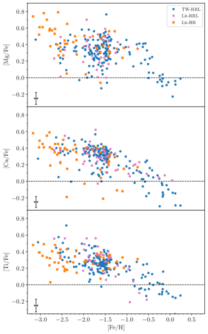
Figure 5: Abundances of Mg, Ca, and Ti for the TW-RRL (blue dots), Lit-RRL (pink dots), and Lit-HB (orange squares) samples. The error bars in the lower left corner of each panel display typical uncertainties.

i) Similar trends for RRL and HB stars – The targets plotted in Fig. 5 come from the same evolutionary path. The current empirical and theoretical evidence indicates that blue HB, RRL and red HB stars are old (t$\geq$ 10 Gyr), low-mass (M$\approx$0.50-0.95M_⊙) stars in their central helium burning phase. They have very similar helium core masses ($\sim$0.50M_⊙) and their key difference is in the envelope mass. A steady decrease in the envelope mass causes a systematic increase in the effective temperature moving the stellar structure from the red HB to the blue HB, passing through the RRL instability strip. There is evidence that some RRLs are the aftermath of close binary evolution and could be younger objects (Pietrzyński et al., 2012; Karczmarek et al., 2017). However, the fraction of RRLs in binary systems is of the order of a few percent (Hajdu et al., 2015; Kervella et al., 2019; Prudil et al., 2019), and the figure for systems with mass transfer is likely to be even more modest. In all our spectroscopic investigations with the present sample, we found no evidence of binarity.

ii) Similar slopes for Mg, Ca, and Ti – The investigated species display a well defined slope when moving from the metal-poor to the metal-rich regime. The steady decrease in $\alpha$-enhancement is more clear in Ti and Ca for which the variation is of the order of $\sim$0.6 dex, but it is also present in Mg. Very metal-poor (Fe/H]$\leq$-2.2) RRLs are strongly enhanced in $\alpha$-elements ([$\alpha$/Fe]$\sim$0.4 to 0.5), while those approaching solar iron abundance are depleted in $\alpha$-elements ([$\alpha$/Fe]$\sim$-0.2 to -0.3, see also Prudil et al. 2020).

iii) Similar dispersion for Ca and Ti – Both Ca and Ti display trends in tight agreement and can be considered the same within uncertainties. Their scatter remains of the order of 0.4 dex over the entire metallicity range and appears to be intrinsic, because it is over 3 times larger than the typical errors (see typical error bars in the bottom left corner of Fig. 5).

The value of the plateau for these two species is not significantly different in our data. It bears mentioning that a disagreement between Ti and Ca in a given investigation may be a consequence of the adopted atomic lines and their transition parameters. Indeed, updated transition parameters derived from laboratory studies are only available for titanium. For calcium, a variety of parameters can be found ranging from laboratory studies dating back to half a century ago to astrophysical determinations that use the Sun or nearby bright stars as a reference. Differences in the adopted lines and their oscillator strengths can result in abundances with variations of the order of 0.2 dex (Pancino et al., 2010). This limitation coupled with smaller sample sizes may have created difficulties in detecting the $\alpha$-element depletion we observe in metal-rich RRLs (e.g. Liu et al., 2013).

iv) Larger dispersion for Mg – Mg shows a large dispersion at metallicities lower than [Fe/H]$\lesssim$-1.2. Measurement difficulties play a role in the scatter. The number of Mg lines is very limited, with mostly strong lines that easily saturate and must be discarded. This means that for several stars the Mg abundance is computed using only one or two transitions. Meanwhile, our spectra typically contained five to 15 lines of varied strengths for Ca and for Ti. As with calcium, magnesium lacks updated transition parameters from laboratory studies. An intrinsic spread, independent of the number of lines and their quality, but rather due to the mechanisms of Mg nucleosynthesis may be present and it is discussed in Sect. 5.4.

5.2 Comparison with different Galactic components

The range in metallicity covered by field RRLs is significantly larger than any other similar datasets in the literature. This is strikingly clear in a comparison with typical stars of different Galactic components, as shown in Fig. 6. The RRLs cover the metal-poor ([Fe/H]$\leq$-2.5) region of the Halo and Bulge, but they also extended to super solar metallicities like the dwarfs and giants in the Thin and Thick Disks.

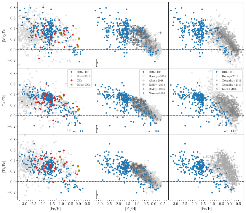
Figure 6: Abundances of Mg, Ca, and Ti for the RRL+HB sample, compared to three typical Galactic populations. Left: Globular clusters and Halo field stars. Middle: Thin and thick disk field stars. Right: Bulge field stars. References – GCs: Pritzl et al. (2005); Carretta et al. (2009a, b, 2010a), Bulge GCs: Gonzalez et al. (2011), The remaining references are labeled according to the first author and year of publication: Frebel (2010), Bensby et al. (2014), Reddy et al. (2003), Reddy et al. (2006), Afsar et al. (2018), Nissen & Schuster (2010), Duong et al. (2019), Gonzalez et al. (2011), Gonzalez et al. (2015), Koch et al. (2016).

As suggested by Nissen & Schuster (2010) and more recently by the near-infrared APOGEE survey Hayes et al. (2018), there is evidence of a bimodal distribution in the [Mg/Fe] versus [Fe/H] plane for metallicities between -1.50 and -0.50 dex. This bimodality is not observed in our data, suggesting that it may an age-related phenomenon. In this same Mg vs iron plane, field RRLs, field stars and GCs attain quite similar values in the Halo, with a dispersion that allows only modest claims about a slope. On the other hand, field RRLs display a well defined slope in Ca and in Ti when moving from [Fe/H]$\approx$-3.2 to -1.3, while field stars and GCs display an almost constant value at $\approx$0.3 dex.

5.3 Comparison with nearby dwarf galaxies

The current Cold Dark Matter cosmological simulations suggest that the Halo formed from the aggregation of protogalactic fragments – small galaxies form first and then merge to form larger galaxies (Dekel & Silk, 1986; Bullock & Johnston, 2005; Monachesi et al., 2019). The discovery of stellar streams and the merging of a massive dwarf galaxy like Sagittarius (Ibata et al., 1994), Gaia Enceladus (Helmi et al., 2018) and Sequoia (Myeong et al., 2019) provided further support to this hierarchical mechanism. Metallicity distribution functions can provide solid quantitative constraints on the mass assembly of the Galactic Halo (Fiorentino et al., 2017), therefore, we also compared the current $\alpha$-element abundances with similar abundances for RGs in nearby dwarf galaxies.

The data plotted in Fig. 7 display the same comparison of Fig. 6, but for $\alpha$-element abundances of individual RG stars in both classical dwarf galaxies and Ultra Faint Dwarfs (UFDs). Note that in this comparison we are only taking into account measurements based on HR spectra.

The samples for Sagittarius and Fornax are marked by red stars and goldenrod diamonds, respectively. The comparison indicates a remarkable agreement in the metal-rich tail ([Fe/H]$\geq$-1.2) between Halo RRLs and RGs in Sagittarius and, in particular, the $\alpha$-poor RRLs approaching solar iron abundance. The trend in the three different $\alpha$-elements are similar across a range in iron abundance of over 1 dex, with marginal variations. In the case of the RGs in Fornax, however, the agreement with the RRL+HB sample is only present for metallicities between -1.3 to -1.8 dex. Indeed, the bulk of Fornax RGs are on overage more $\alpha$-poor than our sample.

A good agreement can also be seen in the metal-poor regime ([Fe/H]$\leq$-2.2) between the RRL+HB sample and RGs in UFDs (grey crosses, data from Vargas et al., 2013). This is quite interesting, because the age distribution in UFDs is narrower when compared to classical dSph galaxies. However, recent spectroscpic measurements are suggesting that the chemical abundance distributions of RGs in UFDs is inhomogeneous (Koch et al., 2008b; Weisz et al., 2014). The empirical framework becomes even more complex for the more massive dwarf galaxies because they exhibit a broad range of star formation histories and chemical enrichment histories (Tolstoy et al., 2009). Indeed, the $\alpha$-element abundances for classical dwarf galaxies (light blue squares) have a dispersion in $\alpha$ abundances, at fixed iron content, that is significantly larger than for our sample. Note that this trend is also caused by the fact that the current $\alpha$-element abundances are restricted, due to an observational bias, to bright RGs in nearby dwarf galaxies. This means that they typically cover a broad range in age. Fabrizio et al. (2015) has recently addressed this issue and found that old and intermediate-age stellar populations in the Carina dSph galaxy display a difference of $\sim$0.6 dex in $\alpha$-element abundances (see also Koch et al., 2008a). Unfortunately, we still lack accurate abundance estimates of $\alpha$-elements in truly old stellar tracers (RRL and non-variable HB stars) belonging to nearby dwarf galaxies to be compared to our sample.

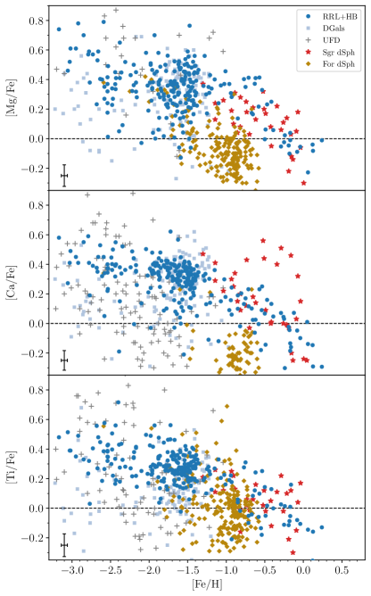
Figure 7: Abundances of Mg, Ca, and Ti for the RRL+HB sample, compared to stars in nearby dwarf galaxies. Red stars: Sagittarius dSph. Goldenrod diamonds: Fornax dSph. Light blue squares: Carina, Draco, Leo I, Sculptor, Sextans, and Ursa Minor. Grey crosses: ultrafaint dwarf galaxies. References – Shetrone et al. (2001), Tolstoy et al. (2003), Geisler et al. (2005), Sbordone et al. (2007), Aoki et al. (2009) Cohen & Huang (2009), Frebel et al. (2010), Carretta et al. (2010b), Letarte et al. (2010), Tafelmeyer et al. (2010), Starkenburg et al. (2013), Vargas et al. (2013), Hendricks et al. (2014b).

5.4 Preliminary circumstantial evidence concerning RRL chemical enrichment

As mentioned in Sect. 5.1, the plateau in the [X/Fe] versus [Fe/H] plane depends on the quality of the adopted atomic transition parameters. This is the reason why we are mainly interested in the trends among the different $\alpha$-elements. Yet, our results show very good agreement among Mg, Ca, and Ti, including the value of the plateau, in accordance with both the data from Frebel (2010) shown in the rightmost panels of Fig. 6. The same agreement is found with the very metal-poor Halo dwarfs and giants investigated by Cayrel et al. (2004). The logarithmic fits of the [X/Fe] versus [Fe/H] planes agree within errors for the three species, and indeed they are nearly identical for Ca and Ti across the whole metallicity range (Fig. 8, bottom panel).

Magnesium displays a larger spread than Ca and Ti for both the RRL and the Lit-HB samples, and for the typical populations of each Galactic component (Fig. 6). An intrinsic spread in Mg and deviations from the trends set by Ca and Ti may be present due to the dependence on progenitor mass and metallicity of the Mg yields. In theoretical models, the yields of Ca and Ti remain similar for wide range of progenitor masses, but the same cannot be said for Mg. The production of the latter significantly increases in progenitors with large stellar masses (35 M_⊙, see Figure 6 of McWilliam, 1997). Moreover, the production of Mg, at fixed stellar mass, depends on the metallicity. Indeed, it shows a marked decrease when moving from metal-poor/metal-intermediate to metal-rich progenitors (see Figures 2 and 4 in Kobayashi et al., 2006).

However, the current data indicate that [Mg/H], [Ca/H], and [Ti/H] vary in lockstep with one another, with negligible differences in their dispersion. Taken at face value, this result points to an early chemical enrichment that appears to be quite homogeneous for these three species over a wide range in iron abundance.

The average [$\alpha$/Fe] versus iron plane is quite homogeneous and properly fit by the logarithmic function

$$\text{[\alpha/Fe]=a+blog(c-[Fe/H])}$$ (1)

with parameters a, b, c, and RMS error as listed in Tab. 7. The fit is shown in both panels of Fig. 8. We found no trends in the residuals of this fit against the pulsational properties, i.e. period and amplitude, of the RRL sample, nor any peculiar behavior when separating RRab and RRc stars. Furthermore, we did not observe a significant change in either the logarithmic fit parameters nor the residuals when removing Mg. As mentioned in Sect.5.1, our spectra have only a small number of Mg lines, and so the weighted average of the three species favours Ca and Ti with their nearly identical trends. As the $\alpha$-elements considered in this work have different formation channels, we included the parameters for the same logarithmic function considering each individual chemical species individually in Tab. 7. The corresponding fits are shown in the bottom panel of Fig. 8.

Table 7: Parameters of the logarithmic fits (Eq. 1).

Fit	a	b	c	RMS
$\alpha$	0.057$\pm$0.064	0.690$\pm$0.108	0.581$\pm$0.190	0.10
Mg	0.175$\pm$0.074	0.498$\pm$0.139	0.479$\pm$0.278	0.16
Ca	0.075$\pm$0.070	0.639$\pm$0.125	0.532$\pm$0.216	0.12
Ti	0.047$\pm$0.070	0.657$\pm$0.124	0.534$\pm$0.211	0.11
Halo	0.237$\pm$0.013	0.229$\pm$0.032	0.270$\pm$0.021	0.19

Note. — The parameters for the $\alpha$, Mg, Ca, and Ti fits were derived using the full RRL+HB sample. The Halo fit was derived considering all objects in the left panels of Fig. 6 with the exception of the RRL+HB sample.

The spread in $\alpha$-abundance steadily decreases when moving from the metal-poor/metal-intermediate into the more metal-rich ([Fe/H]$\geq$-1.0) regime. The Lit-HB sample does not reach higher metallicities, but this change in spread appears even when considering only the RRLs. Indeed, the spread in alpha element abundance decreases from $\sim$0.5 dex to $\sim$0.2 dex. The position of this sharp decrease in $\alpha$-abundance, the so-called ”knee”, is traditionally interpreted as evidence of the growing impact of SNe Ia. While the SNe II, with their short time scales, quickly enrich the interstellar medium with mainly $\alpha$-elements and some iron, the SNe Ia, with much longer time scales, begin to enrich the interstellar medium when it is already at higher metallicities, injecting it with mostly iron and causing a quick decrease of the $\alpha$-to-iron ratio.

The RRL and HB stars appear to be, at fixed iron abundance, more alpha enhanced than typical Halo objects (left panel of Fig. 6) in the metal-poor ([Fe/H]$\leq$=-2.0) regime and more alpha poor than typical Halo objects in the metal-rich ([Fe/H]$\geq$-1.0) regime. Indeed, a fit with the same logarithmic form shown above but applied to these typical Halo objects is indicated by a dashed grey line in both panels of Fig. 8. The corresponding parameters are listed in Tab. 7. This plain evidence could imply that the role played by SNe II in the Halo chemical enrichment was more crucial in the metal-poor than in the metal-intermediate/metal-rich regime.

There is mounting evidence for a sizable sample of metal-rich HB stars that are also $\alpha$-poor (see Figure 12 in Afsar et al., 2018). Indeed, for iron abundances larger than $\approx$-0.2 dex their $\alpha$-element abundance is either solar or lower. This finding together with our results based on RRLs indicates that the chemical enrichment in a significant fraction of metal-rich old field stars was mainly driven by SNe Ia with a minor contribution from SNe II. The lockstep variations we observed for [X/H] for the three species, and in particular the spread in Mg that is comparible to that of the other species (Sect.5.1), point towards an early chemical enrichment driven by a homogeneous initial mass function over a wide range in iron abundance.

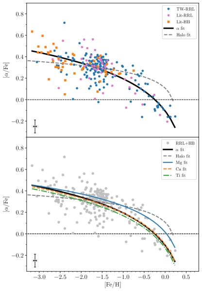
Figure 8: Top: Average [$\alpha$/Fe] abundances using Mg, Ca, and Ti, for the stars in the TW-RRL (blue dots), Lit-RRL (pink dots), and Lit-HB (orange squares) samples. See text for details on the averaging method. The full black line shows the logarithmic fit for the RRL and Lit-HB samples, and the dashed grey line shows the logarithmic fit for the Halo field stars and GCs included the left panels of Fig. 6. Bottom: Same as the top, but with the full RRL+HB sample shown as grey dots. The logarithmic fits for the individual species are shown for Mg (blue solid line), Ca (orange dashed line), and Ti (green dot-dashed line).

6 Summary and future perspectives

We performed the largest and most homogeneous measurement of $\alpha$-element (Mg, Ca, Ti) and iron abundances for field RRLs (162) by using high-resolution spectroscopy. This dataset was complemented with similar abundance estimates available in the literature for 46 field RRLs transformed into our metallicity scale by using objects in common. We ended up with a sample of old (t$\geq$ 10 Gyr) stellar tracers (208 RRLs: 169 RRab, 38 RRc, 1 RRd) covering more than three dex in iron abundance (-3.00$\leq$[Fe/H]$\leq$0.24). Note that the targets were selected to have Galactocentric distances ranging from $\sim$5 to $\sim$ 25 kpc. Therefore, they are solid beacons to investigate the early chemical enrichment of the Galactic Halo.

We found that Mg, Ca, and Ti abundances vary, within the errors, in lock step with one another and have similar scatter over the entire range in iron abundance. Furthermore, the trend in the [$\alpha$/Fe] versus [Fe/H] plane displayed by field RRLs only partially follows the trend typical of other Halo stellar populations. RRLs in the metal-poor regime, appear to be systematically more $\alpha$-enhanced by $\sim$0.1 dex, while in the metal-rich regime they are more $\alpha$-poor by $\sim$0.3 dex, i.e. a factor of three larger than the typical uncertainties. This is the first time this depletion in $\alpha$-elements is detected on the basis of a large, homogeneous and coeval sample of old stellar tracers.

A comparison with nearby classical dwarf galaxies and ultra-faint dwarf galaxies reveals a remarkable agreement between the Halo RRL and RGs in the Sagittarius dSph galaxy in the metal-rich regime. In the the metal-poor regime, beyond the range of the Sagittarius dSph sample, the RRL display a better agreement with the ultra-faint dwarf galaxies than with more massive dwarf galaxies.

To further constrain the role played by stellar age in the early chemical enrichment of the Halo, we took also into account similar elemental abundances for 46 field blue and red HB stars provided by For & Sneden (2010). These stars are either slightly hotter (blue) or slightly cooler (red) than RRLs, however, they share the same evolutionary phase (central helium burning) and the same old (t$\geq$ 10 Gyr), low-mass progenitors. Theory and observations indicate that they only differ in their envelope mass. We found that RRLs and HB stars show the same trends in the [$\alpha$/Fe] versus [Fe/H] planes. These findings support the Halo early chemical enrichment, here traced by unambiguously old stellar tracers.

To overcome the possible occurrence of significant continuum placement uncertainty or saturated lines, we carefully selected lines with equivalent widths between 15 and 150 mÅ. Moreover, we selected several lines that could be measured over a significant fraction of the range in iron covered by the current RRL sample in order to verify that no systematic differences between different lines and chemical species influenced the trend in the [$\alpha$/Fe] versus [Fe/H] plane. Finally, we also performed a comparison with spectroscopic standards (Arcturus) and with field metal-rich red HB stars (Afsar et al., 2018). We found that our iron and $\alpha$-element abundances are, within the errors, in remarkable agreement with similar estimates available in the literature.

Chemical evolution models, for the chemical species discussed in this investigation, point to different dependencies of the yields on the stellar mass and the metallicity regime. This means that the current findings can be soundly adopted to constrain the chemical enrichment history of the Halo. In passing we also note that RRLs and HB stars cover a very narrow range in stellar masses, therefore the comparison with similar Halo stellar tracers can provide useful insights into the role played by the initial mass function and the star formation rate during the Halo early formation.

Our findings concerning the impact that stellar age has on the analysis of the different [$\alpha$/Fe] vs [Fe/H] planes is very promising. New spectroscopic surveys ( WEAVE, Dalton 2016; 4MOST, de Jong et al. 2019; GALAH, De Silva et al. 2015; H3, Conroy et al. 2019; SDSSV, Kollmeier et al. 2017) based on high resolution optical spectra will provide in a few years detailed Halo elemental abundances not only for blue HB and red HB stars, but also for RRLs. This means the unique opportunity to investigate the fine structure in time and in Galactocentric distance of the Halo early chemical enrichment. A similar quantitative jump is also planned for the chemical enrichment of the Galactic Bulge. Thanks to current (APOGEE, Majewski et al. 2017; WINERED, Ikeda et al. 2016) and near future (CRIRES+ at VLT, Follert et al. 2014; MOONS at VLT, Cirasuolo et al. 2014; ERIS at VLT, Davies et al. 2018; PFS at Subaru, Tamura et al. 2018) spectroscopic surveys, detailed elemental abundances will also become available. This means the opportunity to constrain on a quantitative basis the chemical enrichment and the timescale of the Galactic spheroid, i.e. both the Halo and the Bulge.

The current spectroscopic measurements are a fundamental stepping stone for a detailed comparison between chemical evolution models and observations. Indeed, our RRL sample was built to provide a clean (concerning the age distribution) and homogeneous (concerning the methodological approach and the spectroscopic data set) observational framework to compare with theoretical predictions (Cescutti, 2008; Spitoni & Matteucci, 2011; Limongi & Chieffi, 2018).

Appendix A Comparison of equivalent widths

As a simple sanity check, we compared the EWs among pairs of stars with similar effective temperatures and with either similar iron or $\alpha$-abundance (Fig. 9). The number of such pairs is limited due to the need not only of similar T${}_{\text{eff}}$ but also of a significant number of lines in common. The comparison is particularly difficult for stars with lower metallicities or at higher effective temperatures, as they have fewer lines and higher uncertainties overall.

The effective temperature is the parameter that most strongly affects the abundance of each individual line. Thus, a comparison further supports the real variations of [Fe/H] and [$\alpha$/H] among our stars. For a difference of up to approximately 0.15 dex, the EWs for both stars visually coincide. This can be seen in the second row of the left column of Fig. 9. For the other panels, the pair of stars have a difference in either [Fe/H] or [$\alpha$/H] that can be visually detected by the fact that the EWs for the abundance that is similar show an identity relation, while the EWs for abundance that is different are shifted from the identity to either higher or lower values.

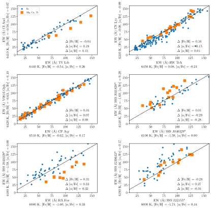
Figure 9: Comparison of equivalent widths for iron (blue dots) and $\alpha$-element (orange squares) lines for stars at similar effective temperatures. The atmospheric parameters of interest for each star are shown in the axes. The difference between [Fe/H], [$\alpha$/H], and [$\alpha$/Fe] are shown on the right left corner of each panel.

Appendix B NLTE corrections and the trend of individual lines

The absorption lines of a given chemical species display equivalent widths that depend on the abundance of the element in question, which is directly related to the overall metallicity [M/H] and, consequently, to the [Fe/H] as well. In other words, the EWs of a given element will be smaller at lower metallicities, and increase with increasing metallicity. This is of particular importance when analysing the [X/Fe] versus [Fe/H] trend because a given line may be too weak at low [Fe/H] or too strong at high [Fe/H], and therefore only measured in a limited range of [Fe/H] values. Using several lines of different strengths ensures that the whole metallicity range is covered, but the transition parameters of different lines are subjected to uncertainties that may result in significant disagreements between them and create spurious trends if one line is only available at lower metallicities, and the other line only at higher metallicities. Therefore, the presence of one single line that covers a wide metallicity range is extremely valuable in order to confirm that any trends are real and not due to such systematics.

A few of the lines adopted in this work cover the entire metallicity range of the current sample. For Mg, no line is present in all metallicity regimes, but the domains of different lines are superposed in such a way that it is possible to verify they are in the same scale. Moreover, the overall behavior of Mg is in agreement with that of Ca and Ti. This is shown in Fig. 10.

Different lines in the same chemical species may be subjected to different levels of NLTE effects. We obtained the values of NLTE corrections using the MPIA NLTE Spectrum Tools. The corrections for Mg (Bergemann et al., 2017), Ca (Mashonkina et al., 2007), and Ti (Bergemann, 2011) lines were computed using 1D plane-parallel models for a set of typical RRL atmospheric parameters in the whole metallicity range covered by our sample. A few lines adopted in this work were not available for this analysis, namely the Mg lines at 8712.69 and 8717.83 Å, the Ca lines at 5581.97, 5601.29, 6471.66, 6493.78, 6499.65, and 6717.69 Å, the TiI lines at 3729.81, 3741.06, 5036.46, and 5038.4 Å, and the TiII lines at 4464.45, 6606.96, and 7214.73 Å. The results for the remaining lines are as follows.

i) Mg: Most corrections for the seven available lines were under $\pm$0.05 dex, with the exception of the metal-poor tail, where four lines had corrections of the order of +0.14.

ii) Ca: Most lines had corrections of the order of a staggering +0.4 dex. However, three lines (6166.4, 6449.8, and 6455.6 Å) display vanishing corrections and yet, in our results, these lines are in good agreement with all others in any given star where they appear. We also note that choosing the spherical 1D models produced corrections as high as 1.0 dex. The source paper for the corrections does not quite cover the atmospheric parameters of RRL, but the closest values provide corrections of the order of 0.2 dex in the metal-poor regime for some of the lines, with smaller positive or negative corrections for the metal-rich regime. We have included the 6455.6 Å line as goldenrod stars in Fig. 10. If the corrections were adopted, this line would remain largely unchanged, while the others were shifted +0.4 dex.

iii) TiI: All available lines displayed corrections of the order of +0.15 dex in the metal-rich regime, increasing to about +0.30 dex in the metal-poor regime. This would further increase the slope in the [TiI/Fe] versus [Fe/H] plane. Interestingly, the results for TiI without any NLTE have a tighter scatter than those for TiII with or without NLTE considerations.

iv) TiII: All available corrections were vanishing, except for a few lines where a shift of the order of +0.12 dex was present in the metal-poor regime. We note, however, that the corrections for the line at 4911.19 Å, shown as goldenrod stars in Fig. 10, were zero.

Without considering the NLTE corrections, a few lines in our sample seem to be systematically higher than others (see e.g. the TiII lines at 4805.09 and 5185.90 Å in Fig. 10), however other lines follow either of the two sequences set by these lines, or remain between them. As the trend in [X/Fe] versus [Fe/H] is the same for both sequences, taking the average value among all lines preserves it, and the higher $\sigma$ of each $\alpha$-element accounts for this decision to include all available lines. The LTE analysis preserves both the internal consistency of our investigation, and the possibility to readily compare it against other data sets in the literature.

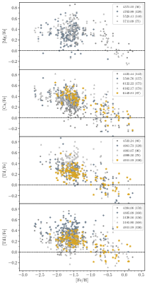
Figure 10: The [X/Fe] versus [Fe/H] trend for individual lines for the three chemical species considered in this work. The lines shown as grey symbols are those with the greatest number of measurments. In red, we show two lines that do not require any NLTE correction. See text for details.

References

- Af\textcommabelowsar et al. (2018) Af\textcommabelowsar, M., Bozkurt, Z., Böcek Topcu, G., et al. 2018, AJ, 155, 240, doi: 10.3847/1538-3881/aabe86
- Alonso et al. (1999) Alonso, A., Arribas, S., & Martínez-Roger, C. 1999, A&AS, 140, 261, doi: 10.1051/aas:1999521
- Alonso et al. (2001) —. 2001, A&A, 376, 1039, doi: 10.1051/0004-6361:20011095
- Aoki et al. (2009) Aoki, W., Arimoto, N., Sadakane, K., et al. 2009, A&A, 502, 569, doi: 10.1051/0004-6361/200911959
- Asplund et al. (2009) Asplund, M., Grevesse, N., Sauval, A. J., & Scott, P. 2009, ARA&A, 47, 481, doi: 10.1146/annurev.astro.46.060407.145222
- Barnes et al. (1988) Barnes, Thomas G., I., Moffett, T. J., Hawley, S. L., Slovak, M. H., & Frueh, M. L. 1988, ApJS, 67, 403, doi: 10.1086/191277
- Bensby et al. (2014) Bensby, T., Feltzing, S., & Oey, M. S. 2014, A&A, 562, A71, doi: 10.1051/0004-6361/201322631
- Bergemann (2011) Bergemann, M. 2011, MNRAS, 413, 2184, doi: 10.1111/j.1365-2966.2011.18295.x
- Bergemann et al. (2017) Bergemann, M., Collet, R., Amarsi, A. M., et al. 2017, ApJ, 847, 15, doi: 10.3847/1538-4357/aa88cb
- Bono (2003) Bono, G. 2003, RR Lyrae Distance Scale: Theory and Observations, ed. D. Alloin & W. Gieren, Vol. 635, 85–104, doi: 10.1007/978-3-540-39882-0_5
- Bono et al. (2020) Bono, G., Braga, V. F., Crestani, J., et al. 2020, ApJ, 896, L15, doi: 10.3847/2041-8213/ab9538
- Bullock & Johnston (2005) Bullock, J. S., & Johnston, K. V. 2005, ApJ, 635, 931, doi: 10.1086/497422
- Cacciari et al. (2000) Cacciari, C., Clementini, G., Castelli, F., & Meland ri, F. 2000, Astronomical Society of the Pacific Conference Series, Vol. 203, Revised Baade-Wesselink Analysis of RR Lyrae Stars, ed. L. Szabados & D. Kurtz, 176–181
- Cacciari et al. (1992) Cacciari, C., Clementini, G., & Fernley, J. A. 1992, ApJ, 396, 219, doi: 10.1086/171711
- Carretta et al. (2009a) Carretta, E., Bragaglia, A., Gratton, R., & Lucatello, S. 2009a, A&A, 505, 139, doi: 10.1051/0004-6361/200912097
- Carretta et al. (2010a) Carretta, E., Bragaglia, A., Gratton, R., et al. 2010a, ApJ, 712, L21, doi: 10.1088/2041-8205/712/1/L21
- Carretta et al. (2009b) Carretta, E., Bragaglia, A., Gratton, R. G., et al. 2009b, A&A, 505, 117, doi: 10.1051/0004-6361/200912096
- Carretta et al. (2010b) —. 2010b, A&A, 520, A95, doi: 10.1051/0004-6361/201014924
- Castelli & Kurucz (2003) Castelli, F., & Kurucz, R. L. 2003, in IAU Symposium, Vol. 210, Modelling of Stellar Atmospheres, ed. N. Piskunov, W. W. Weiss, & D. F. Gray, A20. https://arxiv.org/abs/astro-ph/0405087
- Cayrel et al. (2004) Cayrel, R., Depagne, E., Spite, M., et al. 2004, A&A, 416, 1117, doi: 10.1051/0004-6361:20034074
- Cescutti (2008) Cescutti, G. 2008, A&A, 481, 691, doi: 10.1051/0004-6361:20078571
- Chadid et al. (2017) Chadid, M., Sneden, C., & Preston, G. W. 2017, ApJ, 835, 187, doi: 10.3847/1538-4357/835/2/187
- Cirasuolo et al. (2014) Cirasuolo, M., Afonso, J., Carollo, M., et al. 2014, in Society of Photo-Optical Instrumentation Engineers (SPIE) Conference Series, Vol. 9147, Ground-based and Airborne Instrumentation for Astronomy V, ed. S. K. Ramsay, I. S. McLean, & H. Takami, 91470N, doi: 10.1117/12.2056012
- Clementini et al. (1990) Clementini, G., Cacciari, C., & Lindgren, H. 1990, A&AS, 85, 865
- Clementini et al. (1995) Clementini, G., Carretta, E., Gratton, R., et al. 1995, AJ, 110, 2319, doi: 10.1086/117692
- Cohen (1981) Cohen, J. G. 1981, ApJ, 247, 869, doi: 10.1086/159097
- Cohen & Huang (2009) Cohen, J. G., & Huang, W. 2009, ApJ, 701, 1053, doi: 10.1088/0004-637X/701/2/1053
- Conroy et al. (2019) Conroy, C., Naidu, R. P., Zaritsky, D., et al. 2019, ApJ, 887, 237, doi: 10.3847/1538-4357/ab5710
- Cosentino et al. (2012) Cosentino, R., Lovis, C., Pepe, F., et al. 2012, in Society of Photo-Optical Instrumentation Engineers (SPIE) Conference Series, Vol. 8446, Ground-based and Airborne Instrumentation for Astronomy IV, ed. I. S. McLean, S. K. Ramsay, & H. Takami, 84461V, doi: 10.1117/12.925738
- Crause et al. (2014) Crause, L. A., Sharples, R. M., Bramall, D. G., et al. 2014, in Society of Photo-Optical Instrumentation Engineers (SPIE) Conference Series, Vol. 9147, Ground-based and Airborne Instrumentation for Astronomy V, 91476T, doi: 10.1117/12.2055635
- Crestani et al. (2021) Crestani, J., Fabrizio, M., Braga, V. F., et al. 2021, ApJ, 908, 20, doi: 10.3847/1538-4357/abd183
- Curtis et al. (2019) Curtis, S., Ebinger, K., Fröhlich, C., et al. 2019, ApJ, 870, 2, doi: 10.3847/1538-4357/aae7d2
- Dalton (2016) Dalton, G. 2016, in Astronomical Society of the Pacific Conference Series, Vol. 507, Multi-Object Spectroscopy in the Next Decade: Big Questions, Large Surveys, and Wide Fields, ed. I. Skillen, M. Balcells, & S. Trager, 97
- Davies et al. (2018) Davies, R., Esposito, S., Schmid, H. M., et al. 2018, in Society of Photo-Optical Instrumentation Engineers (SPIE) Conference Series, Vol. 10702, Ground-based and Airborne Instrumentation for Astronomy VII, ed. C. J. Evans, L. Simard, & H. Takami, 1070209, doi: 10.1117/12.2311480
- de Jong et al. (2019) de Jong, R. S., Agertz, O., Berbel, A. A., et al. 2019, The Messenger, 175, 3, doi: 10.18727/0722-6691/5117
- De Silva et al. (2015) De Silva, G. M., Freeman, K. C., Bland-Hawthorn, J., et al. 2015, MNRAS, 449, 2604, doi: 10.1093/mnras/stv327
- Dekel & Silk (1986) Dekel, A., & Silk, J. 1986, ApJ, 303, 39, doi: 10.1086/164050
- Dekker et al. (2000) Dekker, H., D’Odorico, S., Kaufer, A., Delabre, B., & Kotzlowski, H. 2000, in Society of Photo-Optical Instrumentation Engineers (SPIE) Conference Series, Vol. 4008, Optical and IR Telescope Instrumentation and Detectors, ed. M. Iye & A. F. Moorwood, 534–545, doi: 10.1117/12.395512
- Duong et al. (2019) Duong, L., Asplund, M., Nataf, D. M., et al. 2019, MNRAS, 486, 3586, doi: 10.1093/mnras/stz1104
- Fabrizio et al. (2015) Fabrizio, M., Nonino, M., Bono, G., et al. 2015, A&A, 580, A18, doi: 10.1051/0004-6361/201525753
- Fabrizio et al. (2019) Fabrizio, M., Bono, G., Braga, V. F., et al. 2019, ApJ, 882, 169, doi: 10.3847/1538-4357/ab3977
- Fernley & Barnes (1996) Fernley, J., & Barnes, T. G. 1996, A&A, 312, 957
- Fernley et al. (1990) Fernley, J. A., Skillen, I., Jameson, R. F., et al. 1990, MNRAS, 247, 287
- Fiorentino et al. (2015) Fiorentino, G., Bono, G., Monelli, M., et al. 2015, ApJ, 798, L12, doi: 10.1088/2041-8205/798/1/L12
- Fiorentino et al. (2017) Fiorentino, G., Monelli, M., Stetson, P. B., et al. 2017, A&A, 599, A125, doi: 10.1051/0004-6361/201629501
- Follert et al. (2014) Follert, R., Dorn, R. J., Oliva, E., et al. 2014, in Society of Photo-Optical Instrumentation Engineers (SPIE) Conference Series, Vol. 9147, Ground-based and Airborne Instrumentation for Astronomy V, ed. S. K. Ramsay, I. S. McLean, & H. Takami, 914719, doi: 10.1117/12.2054197
- For & Sneden (2010) For, B.-Q., & Sneden, C. 2010, AJ, 140, 1694, doi: 10.1088/0004-6256/140/6/1694
- For et al. (2011) For, B.-Q., Sneden, C., & Preston, G. W. 2011, ApJS, 197, 29, doi: 10.1088/0067-0049/197/2/29
- Frebel (2010) Frebel, A. 2010, Astronomische Nachrichten, 331, 474, doi: 10.1002/asna.201011362
- Frebel et al. (2010) Frebel, A., Simon, J. D., Geha, M., & Willman, B. 2010, ApJ, 708, 560, doi: 10.1088/0004-637X/708/1/560
- Geisler et al. (2005) Geisler, D., Smith, V. V., Wallerstein, G., Gonzalez, G., & Charbonnel, C. 2005, AJ, 129, 1428, doi: 10.1086/427540
- Gonzalez et al. (2011) Gonzalez, O. A., Rejkuba, M., Zoccali, M., et al. 2011, A&A, 530, A54, doi: 10.1051/0004-6361/201116548
- Gonzalez et al. (2015) Gonzalez, O. A., Zoccali, M., Vasquez, S., et al. 2015, A&A, 584, A46, doi: 10.1051/0004-6361/201526737
- Govea et al. (2014) Govea, J., Gomez, T., Preston, G. W., & Sneden, C. 2014, ApJ, 782, 59, doi: 10.1088/0004-637X/782/2/59
- Gratton et al. (2004) Gratton, R., Sneden, C., & Carretta, E. 2004, ARA&A, 42, 385, doi: 10.1146/annurev.astro.42.053102.133945
- Hajdu et al. (2015) Hajdu, G., Catelan, M., Jurcsik, J., et al. 2015, MNRAS, 449, L113, doi: 10.1093/mnrasl/slv024
- Harris (1996) Harris, W. E. 1996, AJ, 112, 1487, doi: 10.1086/118116
- Harris (2010) —. 2010, arXiv e-prints, arXiv:1012.3224. https://arxiv.org/abs/1012.3224
- Hayes et al. (2018) Hayes, C. R., Majewski, S. R., Shetrone, M., et al. 2018, ApJ, 852, 49, doi: 10.3847/1538-4357/aa9cec
- Helmi et al. (2018) Helmi, A., Babusiaux, C., Koppelman, H. H., et al. 2018, Nature, 563, 85, doi: 10.1038/s41586-018-0625-x
- Hendricks et al. (2014a) Hendricks, B., Koch, A., Lanfranchi, G. A., et al. 2014a, ApJ, 785, 102, doi: 10.1088/0004-637X/785/2/102
- Hendricks et al. (2014b) Hendricks, B., Koch, A., Walker, M., et al. 2014b, A&A, 572, A82, doi: 10.1051/0004-6361/201424645
- Ibata et al. (1994) Ibata, R. A., Gilmore, G., & Irwin, M. J. 1994, Nature, 370, 194, doi: 10.1038/370194a0
- Ikeda et al. (2016) Ikeda, Y., Kobayashi, N., Kondo, S., et al. 2016, in Society of Photo-Optical Instrumentation Engineers (SPIE) Conference Series, Vol. 9908, Ground-based and Airborne Instrumentation for Astronomy VI, ed. C. J. Evans, L. Simard, & H. Takami, 99085Z, doi: 10.1117/12.2230886
- Jones et al. (1988) Jones, R. V., Carney, B. W., & Latham, D. W. 1988, ApJ, 326, 312, doi: 10.1086/166093
- Karczmarek et al. (2017) Karczmarek, P., Wiktorowicz, G., Iłkiewicz, K., et al. 2017, MNRAS, 466, 2842, doi: 10.1093/mnras/stw3286
- Kaufer et al. (1999) Kaufer, A., Stahl, O., Tubbesing, S., et al. 1999, The Messenger, 95, 8
- Kervella et al. (2019) Kervella, P., Gallenne, A., Remage Evans, N., et al. 2019, A&A, 623, A116, doi: 10.1051/0004-6361/201834210
- Kobayashi et al. (2006) Kobayashi, C., Umeda, H., Nomoto, K., Tominaga, N., & Ohkubo, T. 2006, ApJ, 653, 1145, doi: 10.1086/508914
- Koch et al. (2008a) Koch, A., Grebel, E. K., Gilmore, G. F., et al. 2008a, AJ, 135, 1580, doi: 10.1088/0004-6256/135/4/1580
- Koch et al. (2008b) Koch, A., McWilliam, A., Grebel, E. K., Zucker, D. B., & Belokurov, V. 2008b, ApJ, 688, L13, doi: 10.1086/595001
- Koch et al. (2016) Koch, A., McWilliam, A., Preston, G. W., & Thompson, I. B. 2016, A&A, 587, A124, doi: 10.1051/0004-6361/201527413
- Kollmeier et al. (2017) Kollmeier, J. A., Zasowski, G., Rix, H.-W., et al. 2017, arXiv e-prints, arXiv:1711.03234. https://arxiv.org/abs/1711.03234
- Lambert et al. (1996) Lambert, D. L., Heath, J. E., Lemke, M., & Drake, J. 1996, ApJS, 103, 183, doi: 10.1086/192274
- Lawler et al. (2013) Lawler, J. E., Guzman, A., Wood, M. P., Sneden, C., & Cowan, J. J. 2013, ApJS, 205, 11, doi: 10.1088/0067-0049/205/2/11
- Lemasle et al. (2014) Lemasle, B., de Boer, T. J. L., Hill, V., et al. 2014, A&A, 572, A88, doi: 10.1051/0004-6361/201423919
- Letarte et al. (2010) Letarte, B., Hill, V., Tolstoy, E., et al. 2010, A&A, 523, A17, doi: 10.1051/0004-6361/200913413
- Limongi & Chieffi (2018) Limongi, M., & Chieffi, A. 2018, ApJS, 237, 13, doi: 10.3847/1538-4365/aacb24
- Liu et al. (2013) Liu, S., Zhao, G., Chen, Y.-Q., Takeda, Y., & Honda, S. 2013, Research in Astronomy and Astrophysics, 13, 1307, doi: 10.1088/1674-4527/13/11/003
- Liu & Janes (1989) Liu, T., & Janes, K. A. 1989, ApJS, 69, 593, doi: 10.1086/191322
- Majewski et al. (2017) Majewski, S. R., Schiavon, R. P., Frinchaboy, P. M., et al. 2017, AJ, 154, 94, doi: 10.3847/1538-3881/aa784d
- Mashonkina et al. (2007) Mashonkina, L., Korn, A. J., & Przybilla, N. 2007, A&A, 461, 261, doi: 10.1051/0004-6361:20065999
- Matteucci & Brocato (1990) Matteucci, F., & Brocato, E. 1990, ApJ, 365, 539, doi: 10.1086/169508
- Matteucci & Greggio (1986) Matteucci, F., & Greggio, L. 1986, A&A, 154, 279
- Mayor et al. (2003) Mayor, M., Pepe, F., Queloz, D., et al. 2003, The Messenger, 114, 20
- McWilliam (1997) McWilliam, A. 1997, ARA&A, 35, 503, doi: 10.1146/annurev.astro.35.1.503
- McWilliam (2016) —. 2016, PASA, 33, e040, doi: 10.1017/pasa.2016.32
- McWilliam et al. (2013) McWilliam, A., Wallerstein, G., & Mottini, M. 2013, ApJ, 778, 149, doi: 10.1088/0004-637X/778/2/149
- Monachesi et al. (2019) Monachesi, A., Gómez, F. A., Grand, R. J. J., et al. 2019, MNRAS, 485, 2589, doi: 10.1093/mnras/stz538
- Myeong et al. (2019) Myeong, G. C., Vasiliev, E., Iorio, G., Evans, N. W., & Belokurov, V. 2019, MNRAS, 488, 1235, doi: 10.1093/mnras/stz1770
- Nissen & Schuster (2010) Nissen, P. E., & Schuster, W. J. 2010, A&A, 511, L10, doi: 10.1051/0004-6361/200913877
- Noguchi et al. (2002) Noguchi, K., Aoki, W., Kawanomoto, S., et al. 2002, PASJ, 54, 855, doi: 10.1093/pasj/54.6.855
- Pancino et al. (2015) Pancino, E., Britavskiy, N., Romano, D., et al. 2015, MNRAS, 447, 2404, doi: 10.1093/mnras/stu2616
- Pancino et al. (2010) Pancino, E., Carrera, R., Rossetti, E., & Gallart, C. 2010, A&A, 511, A56, doi: 10.1051/0004-6361/200912965
- Pietrzyński et al. (2012) Pietrzyński, G., Thompson, I. B., Gieren, W., et al. 2012, Nature, 484, 75, doi: 10.1038/nature10966
- Pilachowski et al. (1983) Pilachowski, C. A., Sneden, C., & Wallerstein, G. 1983, ApJS, 52, 241, doi: 10.1086/190867
- Pritzl et al. (2005) Pritzl, B. J., Venn, K. A., & Irwin, M. 2005, AJ, 130, 2140, doi: 10.1086/432911
- Prudil et al. (2020) Prudil, Z., Dékány, I., Grebel, E. K., & Kunder, A. 2020, MNRAS, 492, 3408, doi: 10.1093/mnras/staa046
- Prudil et al. (2019) Prudil, Z., Skarka, M., Liška, J., Grebel, E. K., & Lee, C. U. 2019, MNRAS, 487, L1, doi: 10.1093/mnrasl/slz069
- Ramírez & Allende Prieto (2011) Ramírez, I., & Allende Prieto, C. 2011, ApJ, 743, 135, doi: 10.1088/0004-637X/743/2/135
- Reddy et al. (2006) Reddy, B. E., Lambert, D. L., & Allende Prieto, C. 2006, MNRAS, 367, 1329, doi: 10.1111/j.1365-2966.2006.10148.x
- Reddy et al. (2003) Reddy, B. E., Tomkin, J., Lambert, D. L., & Allende Prieto, C. 2003, MNRAS, 340, 304, doi: 10.1046/j.1365-8711.2003.06305.x
- Reichert et al. (2020) Reichert, M., Hansen, C. J., Hanke, M., et al. 2020, A&A, 641, A127, doi: 10.1051/0004-6361/201936930
- Salaris & Weiss (1998) Salaris, M., & Weiss, A. 1998, A&A, 335, 943. https://arxiv.org/abs/astro-ph/9802075
- Savino et al. (2020) Savino, A., Koch, A., Prudil, Z., Kunder, A., & Smolec, R. 2020, A&A, 641, A96, doi: 10.1051/0004-6361/202038305
- Sbordone et al. (2007) Sbordone, L., Bonifacio, P., Buonanno, R., et al. 2007, A&A, 465, 815, doi: 10.1051/0004-6361:20066385
- Shetrone et al. (2001) Shetrone, M. D., Côté, P., & Sargent, W. L. W. 2001, ApJ, 548, 592, doi: 10.1086/319022
- Sneden (1973) Sneden, C. 1973, ApJ, 184, 839, doi: 10.1086/152374
- Sneden et al. (1979) Sneden, C., Lambert, D. L., & Whitaker, R. W. 1979, ApJ, 234, 964, doi: 10.1086/157580
- Sneden et al. (2017) Sneden, C., Preston, G. W., Chadid, M., & Adamów, M. 2017, ApJ, 848, 68, doi: 10.3847/1538-4357/aa8b10
- Spitoni & Matteucci (2011) Spitoni, E., & Matteucci, F. 2011, A&A, 531, A72, doi: 10.1051/0004-6361/201015749
- Starkenburg et al. (2013) Starkenburg, E., Hill, V., Tolstoy, E., et al. 2013, A&A, 549, A88, doi: 10.1051/0004-6361/201220349
- Tafelmeyer et al. (2010) Tafelmeyer, M., Jablonka, P., Hill, V., et al. 2010, A&A, 524, A58, doi: 10.1051/0004-6361/201014733
- Tamura et al. (2018) Tamura, N., Takato, N., Shimono, A., et al. 2018, in Society of Photo-Optical Instrumentation Engineers (SPIE) Conference Series, Vol. 10702, Ground-based and Airborne Instrumentation for Astronomy VII, ed. C. J. Evans, L. Simard, & H. Takami, 107021C, doi: 10.1117/12.2311871
- Timmes et al. (1995) Timmes, F. X., Woosley, S. E., & Weaver, T. A. 1995, ApJS, 98, 617, doi: 10.1086/192172
- Tody (1993) Tody, D. 1993, in Astronomical Society of the Pacific Conference Series, Vol. 52, Astronomical Data Analysis Software and Systems II, ed. R. J. Hanisch, R. J. V. Brissenden, & J. Barnes, 173
- Tolstoy et al. (2009) Tolstoy, E., Hill, V., & Tosi, M. 2009, ARA&A, 47, 371, doi: 10.1146/annurev-astro-082708-101650
- Tolstoy et al. (2003) Tolstoy, E., Venn, K. A., Shetrone, M., et al. 2003, AJ, 125, 707, doi: 10.1086/345967
- VandenBerg et al. (2013) VandenBerg, D. A., Brogaard, K., Leaman, R., & Casagrande, L. 2013, ApJ, 775, 134, doi: 10.1088/0004-637X/775/2/134
- Vargas et al. (2013) Vargas, L. C., Geha, M., Kirby, E. N., & Simon, J. D. 2013, ApJ, 767, 134, doi: 10.1088/0004-637X/767/2/134
- Venn et al. (2004) Venn, K. A., Irwin, M., Shetrone, M. D., et al. 2004, AJ, 128, 1177, doi: 10.1086/422734
- Vernet et al. (2011) Vernet, J., Dekker, H., D’Odorico, S., et al. 2011, A&A, 536, A105, doi: 10.1051/0004-6361/201117752
- Walker et al. (2019) Walker, A. R., Martínez-Vázquez, C. E., Monelli, M., et al. 2019, MNRAS, 490, 4121, doi: 10.1093/mnras/stz2826
- Wallerstein et al. (2012) Wallerstein, G., Gomez, T., & Huang, W. 2012, Ap&SS, 341, 89, doi: 10.1007/s10509-012-1033-6
- Wallerstein et al. (1963) Wallerstein, G., Greenstein, J. L., Parker, R., Helfer, H. L., & Aller, L. H. 1963, ApJ, 137, 280, doi: 10.1086/147501
- Wallerstein et al. (1997) Wallerstein, G., Iben, Icko, J., Parker, P., et al. 1997, Reviews of Modern Physics, 69, 995, doi: 10.1103/RevModPhys.69.995
- Weber et al. (2012) Weber, M., Granzer, T., & Strassmeier, K. G. 2012, in Society of Photo-Optical Instrumentation Engineers (SPIE) Conference Series, Vol. 8451, Software and Cyberinfrastructure for Astronomy II, 84510K, doi: 10.1117/12.926525
- Weisz et al. (2014) Weisz, D. R., Dolphin, A. E., Skillman, E. D., et al. 2014, ApJ, 789, 148, doi: 10.1088/0004-637X/789/2/148
- Wood et al. (2013) Wood, M. P., Lawler, J. E., Sneden, C., & Cowan, J. J. 2013, ApJS, 208, 27, doi: 10.1088/0067-0049/208/2/27
- Woosley & Weaver (1995) Woosley, S. E., & Weaver, T. A. 1995, ApJS, 101, 181, doi: 10.1086/192237