Grassmann Iterative Linear Discriminant Analysis with Proxy Matrix Optimization

Abstract

Linear Discriminant Analysis (LDA) is commonly used for dimensionality reduction in pattern recognition and statistics. It is a supervised method that aims to find the most discriminant space of reduced dimension that can be further used for classification. In this work, we present a Grassmann Iterative LDA method (GILDA) that is based on Proxy Matrix Optimization (PMO). PMO makes use of automatic differentiation and stochastic gradient descent (SGD) on the Grassmann manifold to arrive at the optimal projection matrix. Our results show that GILDA outperforms the prevailing manifold optimization method.

1 Introduction

Linear dimensionality reduction is a popular tool used in statistics, machine learning, and signal processing. Linear Discriminant Analysis (LDA) finds the linear projections of high-dimensional data into a low-dimensional space bishop2006pattern and determines the optimal linear decision boundaries in the resulting latent space cunningham2015linear . Fishers LDA fisher1936use ; lda_bio learns the low dimensional space by maximizing the inter-class variability while minimizing the intra-class variability.

LDA is usually solved using the generalized eigenvalue solution, however, this is sub-optimal cunningham2015linear . A better approach would be to cast LDA as an optimization problem over a matrix manifold absil2009optimization . In this paper, we propose the Grassmann Iterative LDA (GILDA) method based on the Proxy Matrix Optimization (PMO) approach Minnehan_2019_CVPR . PMO makes use of Grassmann manifold (GM) optimization combined with a deep learning framework. Previous works have considered the GM in a neural network for various optimization schemes gm_cluster ; gm_sgd ; zhang2018grassmannian . We propose GILDA in a PMO framework and demonstrate improved results over the two-step optimization method in cunningham2015linear . The main contributions of this work are:

• The introduction of a proxy matrix optimization scheme in GILDA to find the optimal projection matrix for LDA.

• Our PMO-based GILDA method outperforms the popular two-step optimization procedure in cunningham2015linear .

• The GILDA framework is suitable for implementation in a neural network with end-to-end training, as it uses automatic differentiation paszke2017automatic and SGD sgd optimization.

2 Background

Linear Discriminant Analysis (LDA) projects labeled data in a lower dimensional space, in a way that maximizes the separation between classes. Let $\textbf{X}=[x_{1},x_{2},\dots,x_{N}]\in\mathbb{R}^{m\times N}$ be the data matrix which is $m$ dimensional and has $N$ data points. To find the LDA projection, the between class scatter matrix ($\mathbf{\Sigma_{B}}$) and the within class scatter matrix ($\mathbf{\Sigma_{W}}$) are calculated as:

$$\mathbf{\Sigma_{W}}=\sum_{i=1}^{n}(x_{i}-\mu_{c_{i}})(x_{i}-\mu_{c_{i}})^{T}\quad\text{ and }\quad\mathbf{\Sigma_{B}}=\sum_{i=1}^{n}(\mu_{c_{i}}-\mu)(\mu_{c_{i}}-\mu)^{T},$$ (1)

where $\mu$ is the mean of the entire dataset and $\mu_{c_{i}}$ is the class mean associated with $x_{i}$. The LDA projection matrix $\textbf{R}\in\mathbb{O}^{m\times p}$ ($p<m$ is the dimension of the lower dimensional space) aims to maximize the between-class variability while minimizing the within-class variability, which leads to minimizing the following objective,

$$f=-\frac{trace(\textbf{R}^{T}\mathbf{\Sigma_{B}}\textbf{R})}{trace(\textbf{R}^{T}\mathbf{\Sigma_{W}}\textbf{R})}.$$ (2)

The projection matrix R is orthogonal under this objective function. The eigenvalue solution considers the top $p$ eigenvectors of the objective ($\mathbf{\Sigma_{W}}^{-1}\mathbf{\Sigma_{B}}$).

3 Manifold Optimization

Manifolds are used in machine learning for dimensionality reduction edelman1998geometry and other applications. The Grassmann manifold $\mathcal{G}^{m\times p}$ hamm_gm ; turaga_gm is of particular interest, because every point on $\mathcal{G}^{m\times p}$ is a linear subspace specified by an orthogonal basis represented by $m\times p$ dimensional matrices edelman1998geometry .

$$\mathcal{G}^{m\times p}\overset{\Delta}{=}\{Span(\textbf{X}):\textbf{X}\in\mathbb{R}^{m\times p},\textbf{X}^{T}\textbf{X}=\textbf{I}_{p}\}$$

Two points on $\mathcal{G}^{m\times p}$ are equivalent if their columns span the same $p$-dimensional subspace edelman1998geometry . The tangent space of the manifold $M$ at a point $\textbf{Y}\in M$ is the linear approximation of the manifold at a particular point and contains all the tangent vectors to $M$ at Y. Mathematically, the tangent space, $T_{Y}M$ is the set of all points X that satisfy $\textbf{Y}^{T}\textbf{X}+\textbf{X}^{T}\textbf{Y}=\textbf{0}_{p}$, where $\textbf{0}_{p}$ is the matrix containing all zero entries. Another important geometric concept is the geodesic, which is the shortest length connecting two points on the manifold.

When optimizing over the Grassmann manifold, the direction of each update step is found in the tangent space of the current location on the manifold. For a given objective $F$, the gradient with respect to a point on the manifold $\textbf{Y}\in M$ is given by:

$$\nabla F=\frac{\partial F}{\partial\mathbf{Y}}-\mathbf{Y}(\frac{\partial F}{\partial\mathbf{Y}})^{T}\mathbf{\mathbf{Y}}^{T}.$$ (3)

The gradient of the loss however is not restricted to the manifold of the tangent space. Thus, it needs to be projected back onto the tangent space. The equation for the projection of a point Z in ambient Euclidean space to the tangent space of the manifold defined at point Y is given by:

$$\pi_{T,{\mathbf{Y}}}({\mathbf{Z}})=\mathbf{Y}\frac{1}{2}(\mathbf{Y}^{T}\mathbf{Z}-\mathbf{Z}^{T}\mathbf{Y})+(\mathbf{I}_{p}-\mathbf{Y}\mathbf{Y}^{T})\mathbf{Z}.$$ (4)

This operation eliminates the components normal to the tangent space while preserving the components on the tangent space of the manifold at point Y. The retraction $r_{p}$ is a mapping from a point in ambient space to the closest point on the manifold: $r_{p}:T_{p}M\rightarrow M$. In this work we use the retraction operation defined by cunningham2015linear which makes use of the SVD of Z, $\textbf{Z}=\textbf{U}\mathbf{\Sigma}\textbf{V}^{T}$ as:

$$r_{\mathbf{p}}(\mathbf{Z})=\mathbf{U}\mathbf{V}^{T}.$$ (5)

The two-step approach for retraction from ambient space on the manifold is used by cunningham2015linear to find the optimal projection matrix. A point $\textbf{R}_{i}$, at iteration $i$, is updated based on the optimization gradients that produce $\textbf{Z}_{i+1}$ in ambient Euclidean space at the next iteration. The point $\textbf{Z}_{i+1}$ is projected to the tangent space using Eq. 4. Following the projection to tangent space, the point is then retracted to the manifold using Eq. 5, resulting in point $\textbf{R}_{i+1}$ on the manifold.

3.1 Proxy Matrix Optimization

The PMO approach in GILDA performs the optimization steps in ambient space, such that each update is in the loss minimizing direction. PMO embeds the manifold retraction inside the optimization function, instead of performing retraction after optimization. Unlike the two-step process, the PMO search is not restricted to the local region of the manifold, and therefore, the extent of the optimization step is not limited. Thus, PMO allows greater steps in ambient space and achieves faster convergence.

The PMO method does not aim to directly optimize a matrix on the manifold, but instead it uses an auxiliary, or Proxy Matrix, that exists in the ambient Euclidean space and is retracted to the closest location on the manifold using Eq. 5. The PMO process is illustrated in Fig. 1 and the corresponding steps are outlined in Algorithm 1. The first step in the PMO process is to retract the proxy matrix, $\mathbf{P_{i}}$ to $\mathbf{Y_{i}}$, its closest location on the manifold. Once the proxy matrix is retracted to the manifold, the loss is calculated based on the loss function at $\mathbf{Y_{i}}$. This loss is then backpropagated through the singular value decomposition of proxy matrix using a method developed by ionescu2015training to a new point $\mathbf{P_{i+1}}$. This point is then retracted back onto the manifold using Eq. 5 to point $\mathbf{Y_{i+1}}$.

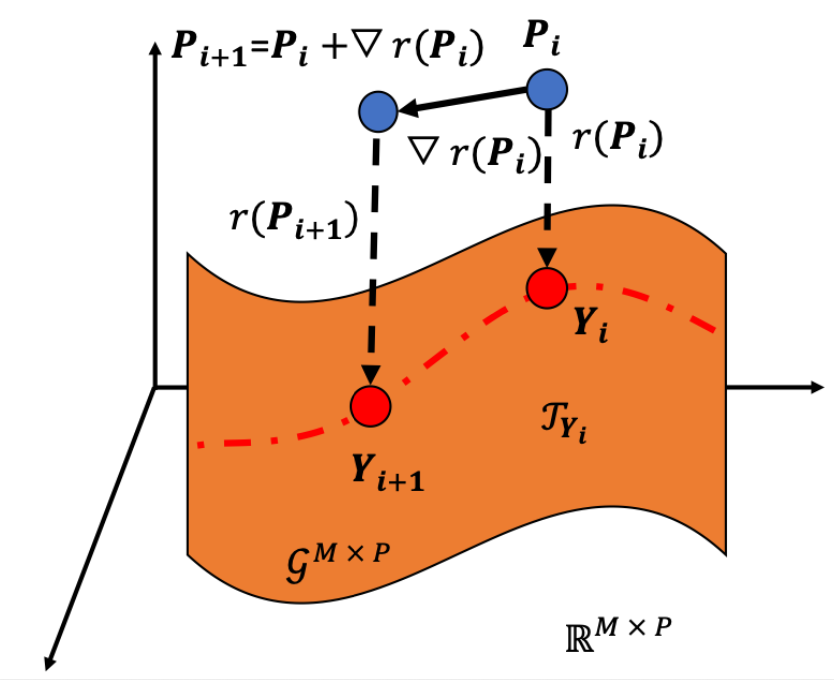
Figure 1: Illustration of the proxy matrix optimization procedure.

Data: $\mathbf{X}\in\mathbb{R}^{m\times N}$

Result: Locally Optimal $\mathbf{P}$ such that $r(\mathbf{P_{i}})$ minimizes the loss $f_{\mathbf{X}}$

initialize $\mathbf{P}\in\mathcal{R}^{m\times p}$ and $\mathbf{P}\not\in\mathcal{G}^{m\times p}$;

for  $i>iter$ do

       $\mathbf{U}\mathbf{S}\mathbf{V}^{T}=\mathbf{P_{i}}$ ;

        /* Retract $\mathbf{P_{i}}$ to $\mathcal{G}^{m\times p}$ */

       $r(\mathbf{P_{i}})=\mathbf{U}\mathbf{V}^{T}$;

       $\nabla r(\mathbf{P_{i}})=\frac{\partial}{\partial\mathbf{P_{i}}}f_{X}(r(\mathbf{P_{i}}))$ ;

        /* Calculate gradients for $\mathbf{P_{i}}$ using Eq.3 */

       $\mathbf{P_{i+1}}=\mathbf{P_{i}}-\mathbf{\beta\nabla r(P_{i})}$ ;

        /* Update $\mathbf{P}$ */

      

end for

Algorithm 1 Proxy Matrix Optimization.

For realization in a deep learning framework, Algorithm 1 is converted into a fully connected layer which is then integrated into a neural network. The dimensionality reduction loss is back-propagated along with the loss corresponding to the network task to obtain the optimal projection matrix. PMO leverages the autograd routine in Pytorch to back-propagate through the SVD and hence removing the need for analytical gradient calculation.

4 Experiments and Results

We perform two experiments to demonstrate the advantage of GILDA and compare our results to the two-step method in cunningham2015linear for the same toy dataset and initial conditions. For the first experiment, data of dimensionality, $d\in[4,8,16,32,64,128,256,512,1024]$ with $N=2000$ points are generated. Each time the data is projected onto a space of dimension $r=3$. The data is normally distributed with random covariance (exponentially distributed eccentricity with mean 2). The metric used to compare the methods is the normalised improvement over the eigenvector objective, described as:

$$-\frac{(f_{X}(\mathbf{R^{(orth)}})-f_{X}(\mathbf{R^{(eig)}}))}{|f_{X}(\mathbf{R^{(eig)}})|},$$ (6)

where $f_{X}$ is the objective function described in Eq. 2, $\mathbf{R^{(orth)}}$ is the projection matrix obtained using our PMO method and $\mathbf{R^{(eig)}}$ is the projection matrix obtained by a tradition eigenvector approach described in Section 2 by orthogonalizing the top $r$ eigenvectors of $\mathbf{\Sigma_{W}}^{-1}\mathbf{\Sigma_{B}}$. We also compare our approach to the two-step method provided by cunningham2015linear using the same metric. The experiments were run 20 times and the results for the two methods are shown in Fig. 2. The results illustrate that for all the experiments, PMO outperforms cunningham2015linear with the added benefit of not having to manually calculate the gradient of the objective function.

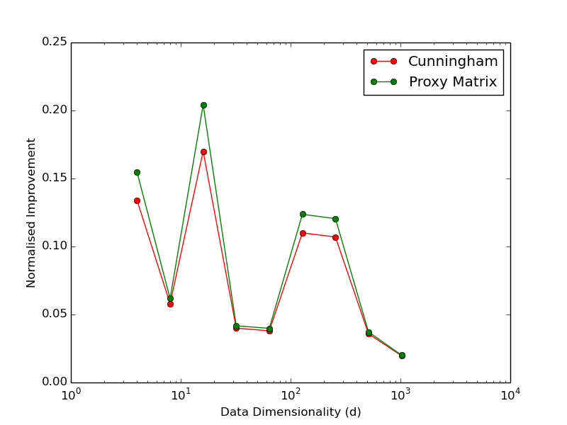
Figure 2: Results from the $d$-sweep experiments using GILDA (with PMO) and two-step cunningham2015linear .

In the second experiment performed, the data dimensionality is fixed at $d=100$ and the projected dimensionality takes on the values of $r\in[1,2,5,10,20,40,80]$ with $n=1000$ data points in each of the $d$ classes. The within class data was generated according to a normal distribution with random covariance (uniformly distributed orientation and exponentially distributed eccentricity with mean 5), and each class mean vector was randomly chosen (normal with standard deviation 5/d). The results of the sweep are shown in Fig. 3. Apart form the case where $r=1$, PMO does better than cunningham2015linear and better than the eigenvector solution.

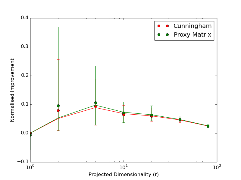
Figure 3: Results from the $r$-sweep experiments using GILDA (with PMO) and two-step cunningham2015linear .

5 Conclusion

We introduced GILDA, a novel method for performing Linear Discriminant Analysis (LDA) using Proxy Matrix Optimization (PMO), that outperforms the popular two-step optimization method and heuristic solutions using eigenvectors. Furthermore, PMO is more functional as it leverages the inbuilt Pytorch SGD routine and automatic differentiation to find the gradients of the loss functions, and is suitable for realization within a deep learning framework. Future work would include integrating the LDA as a layer of a neural network to enable end-to-end training on real world datasets.

References

- (1) C. M. Bishop, Pattern recognition and machine learning. springer, 2006.
- (2) J. P. Cunningham and Z. Ghahramani, “Linear dimensionality reduction: survey, insights, and generalizations.” Journal of Machine Learning Research, vol. 16, no. 1, pp. 2859–2900, 2015.
- (3) R. A. Fisher, “The use of multiple measurements in taxonomic problems,” Annals of Human Genetics, vol. 7, no. 2, pp. 179–188, 1936.
- (4) C. R. Rao, “The utilization of multiple measurements in problems of biological classification,” Journal of the Royal Statistical Society. Series B (Methodological), vol. 10, no. 2, pp. 159–203, 1948. [Online]. Available: http://www.jstor.org/stable/2983775
- (5) P. A. Absil, R. Mahony, and R. Sepulchre, Optimization algorithms on matrix manifolds. Princeton University Press, 2009.
- (6) B. Minnehan and A. Savakis, “Cascaded projection: End-to-end network compression and acceleration,” in Proceedings of the IEEE/CVF Conference on Computer Vision and Pattern Recognition (CVPR), June 2019.
- (7) Q. Wang, J. Gao, and H. Li, “Grassmannian manifold optimization assisted sparse spectral clustering,” in 2017 IEEE Conference on Computer Vision and Pattern Recognition (CVPR), 2017, pp. 3145–3153.
- (8) S. K. Roy, Z. Mhammedi, and M. Harandi, “Geometry aware constrained optimization techniques for deep learning,” in 2018 IEEE/CVF Conference on Computer Vision and Pattern Recognition, 2018, pp. 4460–4469.
- (9) J. Zhang, G. Zhu, R. W. H. J. au2, and K. Huang, “Grassmannian learning: Embedding geometry awareness in shallow and deep learning,” 2018.
- (10) A. Paszke, S. Gross, S. Chintala, G. Chanan, E. Yang, Z. DeVito, Z. Lin, A. Desmaison, L. Antiga, and A. Lerer, “Automatic differentiation in pytorch,” in Advances in Neural Information Processing Systems (NIPS) workshops, 2017.
- (11) H. Robbins and S. Monro, “A stochastic approximation method,” The Annals of Mathematical Statistics, vol. 22, no. 3, pp. 400–407, 1951. [Online]. Available: http://www.jstor.org/stable/2236626
- (12) A. Edelman, T. A. Arias, and S. T. Smith, “The geometry of algorithms with orthogonality constraints,” SIAM journal on Matrix Analysis and Applications, vol. 20, no. 2, pp. 303–353, 1998.
- (13) J. Hamm and D. D. Lee, “Grassmann discriminant analysis: A unifying view on subspace-based learning,” ICML ’08, p. 376–383, 2008. [Online]. Available: https://doi.org/10.1145/1390156.1390204
- (14) P. Turaga, A. Veeraraghavan, and R. Chellappa, “Statistical analysis on stiefel and grassmann manifolds with applications in computer vision,” 26th IEEE Conference on Computer Vision and Pattern Recognition, CVPR, 2008.
- (15) C. Ionescu, O. Vantzos, and C. Sminchisescu, “Training deep networks with structured layers by matrix backpropagation,” arXiv preprint arXiv:1509.07838, 2015.