Safe Affine Transformation-Based Guidance of a Large-Scale Multi-Quadcopter System (MQS)

Abstract

This paper studies the problem of affine transformation-based guidance of a multi-quadcopter system (MQS) in an obstacle-laden environment. Such MQSs can perform a variety of cooperative tasks including information collection, inspection mapping, disinfection, and firefighting. The MQS affine transformation is an approach to a decentralized leader-follower coordination guided by $n+1$ leaders, where leaders are located at vertices of an $n$-D simplex, called leading simplex, at any time $t$. The remaining agents are followers acquiring the desired affine transformation via local communication. Followers are contained in a rigid-size ball at any time $t$ but they can be distributed either inside or outside the leading simplex. By eigen-decomposition of the affine transformation coordination, safety in a large-scale MQS coordination can be ensured by constraining eigenvalues of the affine transformation. Given the initial and final configurations of the MQS, A* search is applied to optimally plan safe coordination of a large-scale MQS minimizing the travel distance between the the initial and final configuration. The paper also proposes a proximity-based communication topology for followers to assign communication weights with their in-neighbors and acquire the desired coordination with minimal computation cost.

I Introduction

Multi-agent coordination has been an active research area in the past few decades and found various applications such as surveillance [1], search and rescue missions [2], agriculture [3], structural health monitoring [4], and air traffic management [5]. Consensus and containment control are common multi-agent coordination approaches that have been extensively studied in the past.

Consensus control is the most well-known decentralized multi-agent coordination approach. Leaderless multi-agent consensus [6, 7] and leader-follower consensus [8] have been previously proposed for multi-agent coordination applications. Multi-agent consensus under fixed communication topology and switching inter-agent communication have been investigated in [9] and [10], respectively. Refs. [11, 12] study stability of the consensus control in the presence of communication delays. Consensus control of a system of nonlinear agents has been investigated in Refs. [13, 14].

Containment control is a leader-follower method in which the group coordination is guided by a finite number of leaders and acquired by followers through local communication. Refs. [15, 16] provide necessary and sufficient conditions for stability and convergence in the multi-agent containment coordination problem. Containment under fixed and switching inter-agent communications are investigated in Refs. [15, 17, 18] Also, multi-agent containment control in the presence of time-varying delays are analyzed in [19, 20]. Refs. [21, 22] have studied finite-time containment control of a multi-agent system.

Continuum deformation is another muti-agent coordination approach that treats agents as particles of a continuum, deforming in a $3$-D motion space. An $n$-D continuum deformation coordination is guided by $n+1$ leaders in a $3$-D motion space where leaders are located at vertices of an $n$-D simplex at any time $t$, and $n\in\{1,2,3\}$. In a continuum deformation coordination, desired trajectories are planned by leaders and acquired by followers through local communication [23]. Therefore, the continuum deformation and containment control are both decentralized leader-follower methods. However, the continuum deformation formally specifies and verifies safety in a large-scale agent coordination by ensuring inter-agent collision avoidance, obstacle collision avoidance, and agent containment [24, 25]. As the result, a large-scale multi-agent system can participate in a continuum deformation coordination mission and the agent team can aggressively deform to pass through the narrow passages in an obstacle-laden environments.

The existing continuum deformation approach [23, 24] requires that the leaders form an $n$-D simplex at any time $t$. This requirement can be quite restrictive when agents are not uniformly distributed at the initial configuration. The main contribution of this paper is to advance the continuum deformation towards affine transformation in which $n+1$ leaders defining the affine transformation coordination form an $m$-D polytope at any time $t$, where $m\leq n\leq 3$. In other words, $n+1$ leaders, guiding the agent coordination, are not required to form an $n$-D simplex at all times $t$. This advancement can significantly improves maneuverability of a large-scale swarm coordination. In particular, our affine transformation-based coordination approach allows to plan more efficient motions than the existing continuum deformation approaches that it extends.

This paper studies the problem of safe and scalable affine transformation of a multi-quadcopter system (MQS) in an obstacle-laden environment (see Fig. 1). Compared to the existing literature and the authors’ previous work, this paper offers the following novel contributions:

1. We decompose the affine transformation coordination problem into spatial and temporal planning problems. For the spatial planning, we use the A* search method to assign the optimal path of quadcopters such that the travel distance between their initial and final positions are minimized, and collision avoidance is guaranteed. For the temporal planning, the MQS travel time is determined such that deviation of every quadcopter from its global desired trajectory, defined by the affine transformation, remains bounded at any time.

2. This paper provides conditions guaranteeing safety in a large-scale affine transformation coordination. By eigen-decomposition of the affine transformation and constraining the deformation eigenvalues of the affine transformation coordination, inter-agent collision avoidance and quadcopter containment are ensured.

3. This paper offers a new proximity-based communication topology for followers to acquire a desired affine transformation through local communication. Our approach is therefore of decentralized type.

The proposed affine transformation approach is particularly appealing for application to smart indoor or outdoor fire-fighting performed by a team of autonomous quadcopters exploiting the proposed approach. In particular, a fire-fighter quadcopter team can effectively coordinate itself in a geometrically-constrained and hazardous environment with minimal human interventions. The fire-fighter quadcopters can deform to pass through narrow channels and quicky react to a rapid growth of fire.

This paper is organized as follows: Preliminaries of the graph theory and motion space discretization are presented in Section II. The problem of affine transformation coordination for a large-scale MQS is stated in Section III. Section VI describes steps to determine (”tune”) [26] algorithm parameters that we used in our case study. More specifically, affine transformation is defined in section IV and inferred via local communication in Section V. Simulation results are presented in Section VI and followed by concluding remarks in Section VII. The proofs are relegated to the Appendix A. Quadcopter modeling details are summarized in Appendices B amd C.

II Preliminaries

II-A Graph Theory Notions

We consider an MQS consisting of $N$ quadcopters moving collectively in a $3$-D space where every quadcopter is uniquely identified by an index number $i\in\mathcal{V}=\{1,\cdots,N\}$ (see Fig. 1). By classifying quadcopters as leaders and followers, $\mathcal{V}$ can be expressed as $\mathcal{V}=\mathcal{V}_{L}\bigcup\mathcal{V}_{F}$, where $\mathcal{V}_{L}=\{1,\cdots,n+1\}$ and $\mathcal{V}_{F}=\mathcal{V}\setminus\mathcal{V}_{L}$ define the leaders’ and followers’ index numbers, respectively, in an $n$-D affine transformation, i.e. $n=1,2,3$. While leaders move independently, followers acquire the desired coordination through local communication. Inter-agent communication is defined by digraph $\mathcal{G}\left(\mathcal{V},\mathcal{E}\right)$ with node set $\mathcal{V}$ and edge set $\mathcal{E}\subset\mathcal{V}\times\mathcal{V}$. Set $\mathcal{V}$ can be expressed as $\mathcal{V}=\mathcal{V}_{B}\bigcup\mathcal{V}_{I}$ where $\mathcal{V}_{B}=\{1,\cdots,N_{B}\}$ and $\mathcal{V}_{I}\{N_{B}+1,\cdots,N\}$ define the index numbers of boundary and interior quadcopters, and $N_{B}\geq n+1$. Given edge set $\mathcal{E}$, the set of in-neighbor quadcopters of quadcopter $i\in\mathcal{V}$ is defined by $\mathcal{N}_{i}=\{j\in\mathcal{V}\big{|}(j,i)\in\mathcal{E}\}$.

Figure 1: Example MQS affine transformation coordination in an obstacle-laden motion space.

II-B Position Notations

This paper studies collective motion of $N$ quadcopters where the position of every quadcopter is expressed with respect to an inertial coordinate system with base vectors $\hat{\mathbf{e}}_{1}=[1\leavevmode\nobreak\ 0\leavevmode\nobreak\ 0]^{T}$, $\hat{\mathbf{e}}_{2}=[0\leavevmode\nobreak\ 1\leavevmode\nobreak\ 0]^{T}$, and $\hat{\mathbf{e}}_{3}=[0\leavevmode\nobreak\ 0\leavevmode\nobreak\ 1]^{T}$. Throughout this paper, $\mathbf{r}_{i,0}=[x_{i,0}\leavevmode\nobreak\ y_{i,0}\leavevmode\nobreak\ z_{i,0}]^{T}$ and $\mathbf{r}_{i,f}=[x_{i,f}\leavevmode\nobreak\ y_{i,f}\leavevmode\nobreak\ z_{i,f}]^{T}$ denote the initial and final positions of quadcopter $i\in\mathcal{V}$ at the initial time $t_{0}$ and at the final time $t_{f}$, respectively. Also, the vector $\mathbf{r}_{i}(t)=[x_{i}(t)\leavevmode\nobreak\ y_{i}(t)\leavevmode\nobreak\ z_{i}(t)]^{T}$ denotes the actual position of quadcopter $i$ at the time instant $t\in[t_{0},t_{f}]$. The global desired position of quadcopter $i\in\mathcal{V}$ is defined by an affine transformation as follows:

$$t\in[t_{0},t_{f}],\qquad\mathbf{r}_{i,a}(t)=\mathbf{Q}(t){\color[rgb]{0,0,0}\left(\mathbf{r}_{i,0}-\mathbf{d}_{0}\right)}+\mathbf{d}\left(t\right),$$ (1)

where $\mathbf{Q}(t)\in\mathbb{R}^{3\times 3}$ is the Jacobian matrix, $\mathbf{d}(t)\in\mathbb{R}^{3\times 3}$ is the rigid-body displacement vector at time $t\in[t_{0},t_{f}]$, and we let $\mathbf{d}_{0}=\mathbf{d}\left(t_{0}\right)$. Furthermore,

$$\mathbf{r}_{i,d}(t)=\begin{cases}\mathbf{r}_{i,a}(t)&i\in\mathcal{V}_{L}\\ \sum_{j\in\mathcal{N}_{i}}w_{i,j}\mathbf{r}_{j}{\color[rgb]{0,0,0}(t)}&i\in\mathcal{V}_{F}\end{cases}.$$ (2)

is called local desired position of quadcopter $i\in\mathcal{V}$ where $w_{i,j}>0$ is the communication weight between follower $i$ and in-neighbor $j\in\mathcal{N}_{i}$ and $\mathbf{r}_{j}(t)$ is the actual position of quadcopter $j$. Note that local and global desired positions of every leader $i\in\mathcal{V}_{L}$ are the same.

Remark 1.

Elements of $\mathbf{Q}{\color[rgb]{0,0,0}(t)}\in\mathbb{R}^{3\times 3}$ and $\mathbf{d}{\color[rgb]{0,0,0}(t)=}\begin{bmatrix}d_{1}(t)&d_{2}(t)&d_{3}(t)\end{bmatrix}^{T}\in\mathbb{R}^{3\times 1}$ can be uniquely related to the global desired positions of $n+1$ leader quadcopters where leader agents form an $n$-D simplex at initial time $t_{0}$ so that:

$$\mathrm{rank}\left(\begin{bmatrix}\mathbf{r}_{2,0}-\mathbf{r}_{1,0}&\cdots&\mathbf{r}_{n+1,0}-\mathbf{r}_{1,0}\end{bmatrix}\right)=n.$$ (3)

Assumption 1.

This paper assumes that quadcopters are initially distributed in an $n$-D hyper-plane defined based on initial positions of leaders $1$ through $n+1$ guiding an $n$-D affine transformation.

Proposition 1.

If Assumption 1 is satisfied and leaders’ initial positions satisfy rank condition (3) at the initial time $t_{0}$, initial position of every quadcopter $i\in\mathcal{V}$ can be uniquely expressed as a linear combination of leaders’ initial positions so that

$$\forall i\in\mathcal{V},\qquad\mathbf{r}_{i,0}=\sum_{j=1}^{n+1}\alpha_{i,j}\mathbf{r}_{j,0},$$ (4)

where

$$\forall i\in\mathcal{V},\qquad\sum_{j=1}^{n+1}\alpha_{i,j}=1.$$ (5)

II-C Rank Operator and Containment Function

Let $\mathbf{p}_{1}$, $\mathbf{p}_{2}$, $\cdots$, $\mathbf{p}_{n+1}$ denote $n+1$ position vectors in a $3$-D motion space. We define the rank function as

$$\varrho_{n}\left(\mathbf{p}_{1},\cdots,\mathbf{p}_{n+1}\right)={\color[rgb]{0,0,0}\mathrm{rank}\left(\begin{bmatrix}\mathbf{p}_{2}-\mathbf{p}_{1}&\cdots&\mathbf{p}_{n+1}-\mathbf{p}_{1}\end{bmatrix}\right)}.$$ (6)

Vectors $\mathbf{p}_{1}$, $\mathbf{p}_{2}$, $\cdots$, $\mathbf{p}_{n+1}$ define vertices of an $n$-D simplex, if $\varrho_{n}\left(\mathbf{p}_{1},\cdots,\mathbf{p}_{n+1}\right)=n$. We also define the containment function as

$$\varkappa_{n}\left(\mathbf{p}_{1},\cdots,\mathbf{p}_{n},\mathbf{c}\right)=\sum_{i=1}^{n+1}\mathrm{sign}\left(\mathbf{D}_{i}\right),$$ (7)

where

$$\mathbf{D}_{i}=\begin{bmatrix}\mathbf{p}_{1}&\cdots&\mathbf{p}_{i-1}&\mathbf{c}&\mathbf{p}_{i+1}&\cdots&\mathbf{p}_{n+1}\\ 1&\cdots&1&1&1&\cdots&1\\ \end{bmatrix}$$ (8)

and $\mathbf{c}\in\mathbb{R}^{3\times 1}$ is the position of an arbitrary point in a $3$-D motion space, $\left|\mathbf{D}_{i}\right|$ is the determinant of matrix $\mathbf{D}_{i}$, and $\mathrm{sign}:\mathbb{R}\rightarrow\left\{-1,0,1\right\}$ is the sign function.

A point $\mathbf{c}$ is inside an $n$-D simplex defined by $\mathbf{p}_{1}$, $\mathbf{p}_{2}$,$\cdots$, $\mathbf{p}_{n+1}$, if $\left|\varkappa_{n}\left(\mathbf{p}_{1},\cdots,\mathbf{p}_{n},\mathbf{c}\right)\right|=n+1$ (See Ref. [24]). Therefore, if $\varkappa_{n}\left(\mathbf{p}_{1},\cdots,\mathbf{p}_{n},\mathbf{c}\right)=n+1$ or $\varkappa_{n}\left(\mathbf{p}_{1},\cdots,\mathbf{p}_{n},\mathbf{c}\right)=-\left(n+1\right)$, then, the point $\mathbf{c}$ is inside the $n$-D simplex defined by $\mathbf{p}_{1}$ through $\mathbf{p}_{n+1}$. The rank function $\varrho_{n}$ and the containment function $\varkappa_{n}$ are used in Section V-A to determine followers’ in-neighbors and communication weights based on local proximity in the MQS initial configuration.

II-D Matrix Decomposition

This paper uses the standard $3-2-1$ Euler angles to define a rotation matrix by

where $C_{\left(\cdot\right)}$ and $S_{\left(\cdot\right)}$ abbreviate $\cos{\left(\cdot\right)}$ and $\sin{\left(\cdot\right)}$, respectively. Also, ${\color[rgb]{0,0,0}X}$, ${\color[rgb]{0,0,0}Y}$, and ${\color[rgb]{0,0,0}Z}$ are the first, second, and third Euler angles where

$$\mathbf{R}\left({\color[rgb]{0,0,0}X},{\color[rgb]{0,0,0}Y},{\color[rgb]{0,0,0}Z}\right)=\mathbf{R}\left({\color[rgb]{0,0,0}X},0,0\right)\mathbf{R}\left(0,{\color[rgb]{0,0,0}Y},0\right)\mathbf{R}\left(0,0,{\color[rgb]{0,0,0}Z}\right).$$ (10)

Now, the Jacobian matrix $\mathbf{Q}(t)$, introduced in Eq. (1), can be represented as follows:

$$\mathbf{Q}(t)=\mathbf{\Phi}\left(\mathbf{\Theta}(t)\right),$$ (11)

where

$$\mathbf{\Theta}(t)=\begin{bmatrix}\lambda_{1}(t)&\cdots&\lambda_{3}(t)&\beta_{1}(t)&\cdots&\beta_{6}(t)\end{bmatrix}^{T}$$ (12)

is called the deformation feature vector, and $\mathbf{\Phi}$ can be decomposed as follows:

$$\mathbf{\Phi}=\mathbf{R}_{r}\mathbf{U}_{D}{\color[rgb]{0,0,0},}$$ (13)

where the matrix $\mathbf{R}_{r}\left(\beta_{1},\beta_{2},\beta_{3}\right)$ is orthonormal, and the deformation matrix $\mathbf{U}_{D}\left(\beta_{4},\beta_{5},\beta_{6},\lambda_{1},\lambda_{2},\lambda_{3}\right)$ is symmetric. The deformation features $\beta_{1}(t)$, $\beta_{2}(t)$, and $\beta_{3}(t)$ are the first, second, and third Euler angles, and

$$\mathbf{R}_{r}=\mathbf{R}\left(\beta_{1}(t),\beta_{2}(t),\beta_{3}(t)\right).$$ (14)

The deformation matrix can be represented as

$$\mathbf{U}_{D}=\mathbf{R}_{u}\mathbf{\Lambda}\mathbf{R}_{u}^{T}{\color[rgb]{0,0,0},}$$ (15)

where

$$\mathbf{R}_{u}=\mathbf{R}\left(\beta_{4},\beta_{5},\beta_{6}\right)$$ (16)

is a rotation matrix, and $\beta_{4}$, $\beta_{5}$, and $\beta_{6}$ are the first, second, and third Euler angles. The matrix

$$\mathbf{\Lambda}=\begin{bmatrix}\lambda_{1}&0&0\\ 0&\lambda_{2}&0\\ 0&0&\lambda_{3}\end{bmatrix}$$ (17)

is diagonal and real.

Remark 2.

The matrix $\mathbf{U}_{D}(t)$ can be expressed as

$$\mathbf{U}_{D}(t)=\sum_{i=1}^{3}\lambda_{i}(t)\hat{\mathbf{u}}_{i}\left(\beta_{4}(t),\beta_{5}(t),\beta_{6}(t)\right)\hat{\mathbf{u}}_{i}^{T}\left(\beta_{4}(t),\beta_{5}(t),\beta_{6}(t)\right),$$ (18)

where

$$i=1,2,3,\qquad\hat{\mathbf{u}}_{i}\left(\beta_{4}(t),\beta_{5}(t),\beta_{6}(t)\right)=\mathbf{R}^{T}\left(\beta_{4}(t),\beta_{5}(t),\beta_{6}(t)\right)\hat{\mathbf{e}}_{i}$$ (19)

is the $i$-th eigenvector of the deformation matrix $\mathbf{U}_{D}(t)$.

Proposition 2.

If $\lambda_{1}(t)=\lambda_{2}(t)=\lambda_{3}(t)=\lambda(t)$ at time $t$, then the matrix $\mathbf{U}_{D}(t)$ simplifies to

$$\mathbf{U}_{D}(t)=\lambda(t)\mathbf{I}_{3}$$ (20)

independent of the values of $\beta_{4}(t)$, $\beta_{5}(t)$, and $\beta_{6}(t)$ at $t$.

III Problem Statement and Solution Approach

This paper considers collective motion of a quadcopter team consisting of $N$ vehicles defined by $\mathcal{V}=\{1,\cdots,N\}$, where quadcopter $i\in\mathcal{V}$ is modeled by

$$\begin{cases}\dot{\mathbf{x}}_{i}=\mathbf{f}_{i}\left(\mathbf{x}_{i}\right)+\mathbf{g}_{i}\left(\mathbf{x}_{i}\right)\mathbf{u}_{i}\\ \mathbf{r}_{i}=\mathbf{C}_{i}\mathbf{x}_{i}\end{cases}.$$ (21)

In (21), $\mathbf{x}_{i}=\begin{bmatrix}\mathbf{r}_{i}^{T}&\dot{\mathbf{r}}_{i}^{T}&\phi_{i}&\theta_{i}&\psi_{i}&{\color[rgb]{0,0,0}\bf{\omega}}_{i}^{T}\end{bmatrix}^{T}$ is the state, $\mathbf{u}_{i}=\begin{bmatrix}p_{i}&\tau_{\phi,i}&\tau_{\theta,i}&\tau_{\psi,i}\end{bmatrix}^{T}$ is the input, $\mathbf{C}_{i}=\begin{bmatrix}\mathbf{I}_{3}&\mathbf{0}_{3\times 9}\end{bmatrix}$,

where $m_{i}$ and $\mathbf{J}_{i}$ are the mass and mass moment of inertia of quadcopter $i\in\mathcal{V}$, respectively, $\mathbf{0}_{3\times 1}\in\mathbb{R}^{3\times 1}$, $\mathbf{0}_{3\times 3}\in\mathbb{R}^{3\times{\color[rgb]{0,0,0}3}}$, and $\mathbf{0}_{3\times 9}\in\mathbb{R}^{3\times{\color[rgb]{0,0,0}9}}$ are the zero-entry matrices, $\mathbf{I}_{3}\in\mathbb{R}^{3\times 3}$ is the identity matrix, $g=9.81m/s^{2}$ is the gravity, $\mathbf{u}_{i}=\begin{bmatrix}p_{i}&\tau_{\phi,i}&\tau_{\theta,i}&\tau_{\psi,i}\end{bmatrix}^{T}$, and $\mathbf{\Gamma}_{i}\left(\phi_{i},\theta_{i},\psi_{i}\right)$ is defined in Eq. (83) in Appendix B.

The quadcopter team is positioned in an $n$-D hyper plane ($n=1,2,3$) at initial time $t_{0}$ and the MQS initial formation is defined by set $\mathbf{\Omega}_{0}=\{\mathbf{r}_{1,0},\cdots\mathbf{r}_{N,0}\}$ at time $t_{0}$. It is desired that the MQS ultimately forms the desired configuration specified by $\mathbf{\Omega}_{f}=\{\mathbf{r}_{1,f},\cdots\mathbf{r}_{N,f}\}$. where

$$\forall i\in\mathcal{V},\qquad\mathbf{r}_{i,f}={\color[rgb]{0,0,0}\bar{\mathbf{Q}}}_{f}\mathbf{r}_{i,0}+{\color[rgb]{0,0,0}\bar{\mathbf{d}}}_{f},$$ (22)

and where the matrix ${\color[rgb]{0,0,0}\bar{\mathbf{Q}}_{f}}\in\mathbb{R}^{3\times 3}$ and vector ${\color[rgb]{0,0,0}\bar{\mathbf{d}}}_{f}\in\mathbb{R}^{3\times 1}$ are known at time $t_{f}$, and the global desired trajectory of agent $i\in\mathcal{V}$ is defined by Eq. (1) for $t\in[t_{0},t_{f}]$. To ensure safety, we require that the MQS remains inside the rigid containment ball

$$\bar{\mathcal{S}}(t)=\left\{\mathbf{r}\in\mathbb{R}^{3}\big{|}\|\mathbf{r}-\left(\mathbf{d}(t)\right)\|\leq r_{\mathrm{max}}\right\}$$ (23)

at any time $t\in[t_{0},t_{f}]$.

Figure 2: Block diagram of the MQS collective dynamics with the proposed approach.

Given the above problem setup, this paper offers a solution shown in Fig. 2 to safely plan affine transformation of a large-scale quadcopter team by addressing the following two problems:

Problem 1: Affine Transformation Determination: We determine a safe MQS affine transformation by specifying the Jacobian matrix $\mathbf{Q}(t)$ and the rigid-body displacement vector $\mathbf{d}(t)$ such that the travel distance between the initial and final configurations of the MQS is minimized in a geometrically-constrained motion space (see Fig. 1). We assume that every quadcopter can be enclosed by a ball of radius $\epsilon$, and define the matrix $\mathbf{Q}(t)$ over the time interval $[t_{0},t_{f}]$ such that no quadcopter collides with obstacles, or with other quadcopters, and followers do not leave the containment ball $\bar{\mathcal{S}}(t)$ defined by (23) at any time $t\in[t_{0},t_{f}]$. Furthermore, we seek to determine the rigid-body displacement vector $\mathbf{d}$ minimizing the travel distance between the specified initial and final conditions: $\bar{\mathbf{Q}}_{0}=\mathbf{Q}(t_{0})$, $\bar{\mathbf{d}}_{0}=\mathbf{d}(t_{0})$, $\bar{\mathbf{Q}}_{f}=\mathbf{Q}(t_{f})$, $\bar{\mathbf{d}}_{f}=\mathbf{d}(t_{f})$.

Problem 2: Affine Transformation Acquisition: We seek to develop a decentralized method for acquiring the desired affine transformation with local communication. In particular, inter-agent communication and communication weights are assigned based on local proximity. Furthermore, we provide a condition guaranteeing stability of the decentralized affine transformation coordination. We also seek to ensure the boundedness of the deviation of the quadcopter team from a desired affine tranformation coordination by choosing a sufficiently large travel time between in the initial and final MQS configurations.

IV Problem 1: Affine Transformation Definition

An $n$-D affine transformation is defined by planning the trajectory of the rigid-body displacement vector $\mathbf{d}(t)$ and deformation vector $\mathbf{\Theta}(t)$ over the time-interval $t\in[t_{0},t_{f}]$ as described in Sections IV-A and IV-B

IV-A Planning of Rigid-Body Displacement Vector $\mathbf{d}$

Given the initial and final displacement vectors $\bar{\mathbf{d}}_{0}$ and $\bar{\mathbf{d}}_{f}$, we use the the A* search to determine $n_{\tau}-1$ intermediate waypoints $\bar{\mathbf{d}}_{1}$, $\cdots$, $\bar{\mathbf{d}}_{n_{\tau}-1}$. The objective of the A* planner is to minimize the travel distance of the containment ball in an obstacle-laden motion space while ensuring collision avoidance.

Given the optimal waypoints $\bar{\mathbf{d}}_{0}$, $\cdots$, $\bar{\mathbf{d}}_{n_{\tau}}$ ($\bar{\mathbf{d}}_{n_{\tau}}=\bar{\mathbf{d}}_{f}$), we define

$$\mu_{l}=\dfrac{\|\bar{\mathbf{d}}_{l+1}-\bar{\mathbf{d}}_{l}\|}{\sum_{l=0}^{n_{\tau}-1}\|\bar{\mathbf{d}}_{l+1}-\bar{\mathbf{d}}_{l}\|}.$$ (24)

for $l=0,1,\cdots,n_{\tau}-1$. In this paper,

$$T_{l}=\mu_{l}\left(t_{n_{\tau}}-t_{0}\right)$$ (25)

is considered as the travel time between two consecutive waypoints $\bar{\mathbf{d}}_{l}$ and $\bar{\mathbf{d}}_{l+1}$, where $t_{n_{\tau}}=t_{f}$ is free. The rigid body displacement vector $\mathbf{d}(t)$ is defined by

$$\mathbf{d}(t)=\begin{cases}\bar{\mathbf{d}}_{l}\left(1-\gamma\left(t,T_{l}\right)\right)+\gamma\left(t,T_{l}\right)\bar{\mathbf{d}}_{l+1}&t_{l}\leq t<t_{l+1},\leavevmode\nobreak\ l<n_{\tau}\\ \bar{\mathbf{d}}_{n_{\tau}}&t=n_{\tau}=t_{f}\end{cases}$$ (26)

where $T_{l}=t_{l+1}-t_{l}$ is the travel time between $\bar{\mathbf{d}}_{l}$ and $\bar{\mathbf{d}}_{l+1}$, $\bar{\mathbf{d}}_{n_{\tau}}=\mathbf{d}_{f}$, and $\gamma(t,T_{l})$ is defined as follows:

$$t\in[t_{l},t_{l+1}],\qquad\gamma(t,T_{l})=\sum_{j=0}^{5}\zeta_{j}\left({t-{\color[rgb]{0,0,0}t_{l}}\over T_{l}}\right)^{j}$$ (27)

for $l=0,\cdots,n_{\tau-1}$. Here $\zeta_{0}$ through $\zeta_{5}$ are constant coefficients, and $T_{l}=t_{l+1}-t_{l}$. Therefore, the containment ball moves on a straight path at every time $t\in[t_{l},t_{l+1}]$ where $\gamma(t_{l},T_{l})=0$ and $\gamma(t_{l+1},T_{l})=1$ for every $T_{l}>0$ and $l=0,\cdots,n_{\tau}-1$.

IV-B Planning of Deformation Feature Vector Trajectory $\mathbf{\Theta(t)}$

By using Eq. (11), $\mathbf{Q}(t)$ can be expressed as $\mathbf{Q}(t)=\mathbf{\Phi}\left(\mathbf{\Theta}(t)\right)$, and assigned by planning of the deformation vector $\mathbf{\Theta}(t)$ over the time-interval $[t_{0},t_{f}]$. The deformation feature vector $\mathbf{\Theta}:\left[t_{0},t_{f}\right]\rightarrow\mathbb{R}^{6\times 1}$ is defined as follows:

$$\mathbf{\Theta}(t)=\begin{cases}\bar{\mathbf{\Theta}}_{l}\left(1-\gamma\left(t,T_{l}\right)\right)+\gamma\left(t,T_{l}\right)\bar{\mathbf{\Theta}}_{l+1}&t_{l}\leq t<t_{l+1},\leavevmode\nobreak\ l<n_{\tau}\\ \bar{\mathbf{\Theta}}_{n_{\tau}}&t=n_{\tau}=t_{f}\end{cases},$$ (28)

where initial and final conditions

$$\bar{\mathbf{\Theta}}_{0}=\mathbf{\Theta}\left(t_{0}\right)=\begin{bmatrix}\lambda_{1,0}&\lambda_{2,0}&\lambda_{3,0}&\beta_{1,0}&\cdots&{\color[rgb]{0,0,0}\beta_{6,0}}\end{bmatrix}^{T},$$ (29a)

$$\bar{\mathbf{\Theta}}_{f}=\mathbf{\Theta}\left(t_{f}\right)=\begin{bmatrix}\lambda_{1,f}&\lambda_{2,f}&\lambda_{3,f}&\beta_{1,f}&\cdots&\beta_{6,f}\end{bmatrix}^{T}$$ (29b)

are known, and

$$\bar{\mathbf{\Theta}}_{l}=\bar{\mathbf{\Theta}}_{0}+\mu_{l}\left(\bar{\mathbf{\Theta}}_{f}-\bar{\mathbf{\Theta}}_{0}\right).$$ (30)

Note that function $\gamma(t,T_{l})$ is defined in Eq. (27).

IV-B1 Deformation Angles $\beta_{4}$, $\beta_{5}$ and $\beta_{6}$

There is no constraint on selecting $\beta_{4,0}$, $\beta_{5,0}$, $\beta_{6,0}$, and they can be arbitrarily because $\lambda_{1,0}=\lambda_{2,0}=\lambda_{3,0}=1$. In this paper, we let shear deformation angles $\beta_{5}(t)$ and $\beta_{6}(t)$ be constant over time, and assign them based on the initial positions of the quadcopters by solving the following max-min optimization problem:

$$\left(\beta_{5,0},\beta_{6,0}\right)=\operatorname*{\arg\!\max}\limits_{\beta_{5},\beta_{6}}\left\{\min\limits_{i,j\in\mathcal{V},\leavevmode\nobreak\ i\neq j}\left\{\left(\mathbf{r}_{i,0}-\mathbf{r}_{j,0}\right)\cdot\hat{\mathbf{u}}_{1}\left(0,\beta_{5},\beta_{6}\right)\right\}\right\}.$$ (31)

Note that $\hat{\mathbf{u}}_{1,0}$ is independent of $\beta_{4,0}$ and hence we choose $\beta_{4,0}=0$ without loss of generality. Therefore,

$$\hat{\mathbf{u}}_{1,0}=\begin{bmatrix}\cos\beta_{5,0}\cos\beta_{6,0}&\cos\beta_{5,0}\sin\beta_{6,0}&-\sin\beta_{5,0}\end{bmatrix}^{T},$$ (32a)

$$\hat{\mathbf{u}}_{2,0}=\begin{bmatrix}\sin\beta_{6,0}&\cos\beta_{6,0}&0\end{bmatrix}^{T},$$ (32b)

$$\hat{\mathbf{u}}_{3,0}=\begin{bmatrix}\sin\beta_{5,0}\cos\beta_{6,0}&\sin\beta_{5,0}\sin\beta_{6,0}&\cos\beta_{5,0}\end{bmatrix}^{T}$$ (32c)

are the eigenvectors of deformation matrix $\mathbf{U}_{D}(t)$ at any time $t\in[t_{0},t_{f}]$.

Remark 3.

Deformation angles $\beta_{5,0}$ and $\beta_{6,0}$ are assigned such that the unit vector $\hat{\mathbf{u}}_{1,0}$ is along the line connecting the two quadcopters identified by solving (31).

IV-B2 Eigenvalues $\lambda_{1}$, $\lambda_{2}$, and $\lambda_{3}$

Theorem 1 is provided in this section to ensure inter-agent collision avoidance and quadcopter containment by assigning lower and upper bounds on eigenvalues $\lambda_{1}$, $\lambda_{3}$, and $\lambda_{3}$.

Definition 1.

The minimum global separation distance in an affine transformation is defined by

$$d_{\mathrm{min}}=\min\limits_{i,j\in\mathcal{V},\leavevmode\nobreak\ i\neq j}\left\{\left(\mathbf{r}_{i,0}-\mathbf{r}_{j,0}\right)\cdot\hat{\mathbf{u}}_{1}\left(0,\beta_{5},\beta_{6}\right)\right\}.$$ (33)

Definition 2.

The maximum global separation distance in an affine transformation is defined as

$$d_{\mathrm{max}}=\max\limits_{i\in\mathcal{V}}=\|\mathbf{r}_{i,0}-\bar{\mathbf{d}}_{0}\|_{2}.$$ (34)

Theorem 1.

Assume every quadcopter is enclosed by a ball of radius $\epsilon$, and the control input $\mathbf{u}_{i}$ is designed such that

$$\|\mathbf{r}_{i}(t)-\mathbf{r}_{i,a}(t)\|\leq\delta$$ (35)

at any time $t\in[t_{0},t_{f}]$ where $\delta>0$ is constant. Inter-agent collision avoidance and quadcopter containment conditions, specified by

$$\forall t\in\left[t_{0},t_{f}\right],\qquad\bigwedge_{i=1}^{N-1}\bigwedge_{j=i+1}^{N}\left(\|\mathbf{r}_{i}(t)-\mathbf{r}_{j}(t)\|>2\epsilon\right),$$ (36a)

$$\forall t\in\left[t_{0},t_{f}\right],\qquad\bigwedge_{i=1}^{N}\left(\mathbf{r}_{i}(t)\in\bar{\mathcal{S}}(t)\right)$$ (36b)

are guaranteed, if

$$\forall t\in[t_{0},t_{f}],\qquad\lambda_{1}(t)>\lambda_{\mathrm{min}},$$ (37a)

$$\forall t\in[t_{0},t_{f}],\leavevmode\nobreak\ i=1,2,3,\qquad\left|\lambda_{i}(t)\right|\leq\lambda_{\mathrm{max}},$$ (37b)

where

$$\lambda_{\mathrm{min}}=\dfrac{2\left(\delta+\epsilon\right)}{d_{\mathrm{min}}},$$ (38a)

$$\lambda_{\mathrm{max}}=\dfrac{r_{\mathrm{max}}-\delta-\epsilon}{d_{\mathrm{max}}}.$$ (38b)

Note that inter-agent collision avoidance is guaranteed only by imposing constraint (37a) on eigenvalue $\lambda_{1}$. However, all eigenvalues of matrix $\mathbf{U}_{D}(t)$ must satisfy safety condition (37b) to ensure no quadcopter leaves the containment ball $\bar{\mathcal{S}}(t)$ at any time $t\in[t_{0},t_{f}]$.

Remark 4.

While $\lambda_{1,0}=\lambda_{2,0}=\lambda_{3,0}=1$, $\lambda_{1,f}$, $\lambda_{2,f}$, and $\lambda_{3,f}$ need to be selected such that Eq. (22) is satisfied, and

$$i=1,2,3,\qquad\left|\lambda_{i,f}\right|\leq\lambda_{\mathrm{max}}.$$ (39)

IV-B3 Rotation angles $\beta_{1}$, $\beta_{2}$, and $\beta_{3}$

The initial values of rotation angles $\beta_{1}$, $\beta_{2}$, and $\beta_{3}$, denoted by $\beta_{1,0}$, $\beta_{2,0}$, $\beta_{3,0}$, can be arbitrarily selected. However, $\beta_{1,f}$, $\beta_{2,f}$, $\beta_{3,f}$ need to be selected such that Eq. (22) is satisfied.

V Problem 2: Affine Transformation Acquisition

In this paper, a desired affine transformation is acquired in a decentralized fashion via local communication. A proximity-based communication topology is developed in Section V-A to (i) classify quadcopters into followers and leaders and (ii) determine in-neighbor quadcopters of every follower quadcopter $i\in\mathcal{V}_{F}$. MQS collective dynamics are then obtained in Section V-B and followed by analysis of stability and boundedness of the MQS collective dynamics in Sections V-B2 and V-C, respectively.

V-A Proximity-Based Inter-Agent Communication

In a decentralized affine transformation coordination, leaders move independently therefore $\mathcal{N}_{i}=\emptyset$ if $i\in\mathcal{V}_{L}$. Non-leader boundary quadcopters, defined by $\mathcal{V}_{B}$, directly communicate with leaders. Therefore,

$$i\in\mathcal{V}_{B}\setminus\mathcal{V}_{L},\qquad\mathcal{N}_{i}=\mathcal{V}_{L}.$$ (40)

In-neighbors of the interior quadcopters, defined by $\mathcal{V}_{I}$, are assigned based on local proximity. For every quadcopter $i\in\mathcal{V}_{I}$, we define $l_{i}$-proximity set

$$\begin{split}\mathcal{W}_{i,n}\left(l_{i}\right)=&\bigg{\{}\left(i_{1},\cdots,i_{n+1}\right)\in\mathcal{V}^{n+1}\big{|}\left(\bigwedge_{k=1}^{n+1}\|\mathbf{r}_{i_{k},0}-\mathbf{r}_{i,0}\|\leq l_{i}\right)\wedge\\ &\left(\left|\varkappa_{n}\left(\mathbf{r}_{i_{1},0},\cdots,\mathbf{r}_{i_{n+1},0},\mathbf{r}_{i,0}\right)\right|=n+1\right)\bigg{\}}\end{split}$$ (41)

as the set of all $n$-D simplexes that are inside the ball of radius $l_{i}$ with the center positioned at $\mathbf{r}_{i,0}$. Then, the minimum proximity distance $l_{i}^{*}$ is assigned by solving the following optimization problem:

$$\min l_{i}$$ (42)

such that

$$\mathcal{W}_{i}\left(l_{i}\right)\neq\emptyset.$$ (43)

Remark 5.

If $\left|\mathcal{W}_{i}\left(l_{i}^{*}\right)\right|=1$, then, $\mathcal{W}_{i}=\{\mathcal{N}_{i}\}$.

Assumption 2.

If $\left|\mathcal{W}_{i}\left(l_{i}^{*}\right)\right|>1$, any collection of $n+1$ quadcopters belonging to set $\mathcal{W}_{i}\left(l_{i}^{*}\right)$ can be selected as in-neighbors of interior agent $i\in\mathcal{V}_{I}$.

Let the communication weight of follower quadcopter $i\in\mathcal{V}_{F}$ with in-neighbor quadcopter $j\in\mathcal{N}_{i}$ is denoted by $w_{i,j}$. Let $N_{i}=\{i_{1},\cdots,i_{n+1}\}$ define in-neighbors of follower $i\in\mathcal{V}_{F}$, then, the local desired trajectory of quadcopter $i\in\mathcal{V}_{F}$ is given by

$$\forall t\in[t_{0},t_{f}],i\in\mathcal{V}_{F},\qquad\mathbf{r}_{i,d}(t)=\sum_{k=1}^{n+1}w_{i,k}\mathbf{r}_{i_{k}}(t),$$ (44)

where $\mathbf{r}_{i_{k}}(t)$ denotes the actual position of in-neighbor $i_{k}\in\mathcal{N}_{i}$ ($k=1,\cdots,n+1$). Communication weights of follower $i\in\mathcal{V}_{F}$ are defined as [23, 24]

$$\begin{bmatrix}w_{i,i_{2}}\\ \vdots\\ w_{i,i_{n+1}}\end{bmatrix}=\begin{bmatrix}\mathbf{r}_{i_{2},0}-\mathbf{r}_{i_{1},0}&\cdots&\mathbf{r}_{i_{n+1},0}-\mathbf{r}_{i_{1},0}\end{bmatrix}^{-1}\mathbf{r}_{i,0},$$ (45a)

$$w_{i,i_{1}}=1-\sum_{k=2}^{n+1}w_{i,i_{k}}.$$ (45b)

Given followers’ communication weights, weight matrix $\mathbf{W}=[W_{ij}]\in\mathbb{R}^{N\times N}$ is defined as follows:

$$W_{ij}=\begin{cases}w_{i,j}&i\in\mathcal{V}_{F},\leavevmode\nobreak\ j\in\mathcal{N}_{i}\\ 0&\mathrm{otherwise}\end{cases}.$$ (46)

The matrix $\mathbf{W}$ can be partitioned as follows:

$$\mathbf{W}=\left[\begin{array}[]{c|c}\mathbf{0}&\mathbf{0}\\ \hline\cr\mathbf{F}&\mathbf{G}\end{array}\right]\in\mathbb{R}^{N\times N},$$ (47)

where $\mathbf{F}\in\mathbb{R}^{\left(N-n-1\right)\times\left(n+1\right)}$; matrix $\mathbf{G}\in\mathbb{R}^{\left(N-n-1\right)\times\left(N-n-1\right)}$ is non-negative.

Theorem 2.

Assume inter-agent communication is defined by graph $\mathcal{G}\left(\mathcal{V},\mathcal{E}\right)$ with node set $\mathcal{V}$ and edge set $\mathcal{E}\subset\mathcal{V}\times\mathcal{V}$, where $\mathcal{V}=\mathcal{V}_{B}\bigcup\mathcal{V}_{I}$; $\mathcal{V}_{B}=\{1,\cdots,N_{B}\}$ and $\mathcal{V}_{I}=\{N_{B}+1,\cdots,N\}$ define index numbers of boundary and interior agents, respectively. If leaders defined by set $\mathcal{V}_{L}=\{1,\cdots,n+1\}\subset\mathcal{V}_{B}$ moves independently, non-leader boundary agents defined by $\mathbf{V}_{B}\setminus\mathcal{V}_{L}$ all communicate with leaders, followers’ in-neighbors are determined by solving the optimization problem given in (42) and (43), and followers communication weights are defined based on agents’ initial positions using relation (45), then, the matrix

$$\mathbf{L}=-\mathbf{I}+\mathbf{W}$$ (48)

is Hurwitz.

Let

$$\mathbf{Y}_{a}(t)=\mathrm{vec}\left(\begin{bmatrix}\mathbf{r}_{1,a}(t)&\cdots&\mathbf{r}_{N,a}(t)\end{bmatrix}^{T}\right)$$ (49)

aggregate global desired positions of all quadcopters at time $t$ and

$$\mathbf{R}_{L}(t)=\mathrm{vec}\left(\begin{bmatrix}\mathbf{r}_{1,a}(t)&\cdots&\mathbf{r}_{n+1,a}(t)\end{bmatrix}^{T}\right)$$ (50)

aggregate global desired positions of all leaders at time $t$, where $\mathrm{vec}\left(\cdot\right)$ is the matrix vectorization operator. Vectors $\mathbf{Y}_{a}(t)$ and $\mathbf{R}_{L}(t)$ are related by [24]

$$\mathbf{Y}_{a}(t)=\left(\mathbf{I}_{3}\otimes\mathbf{H}\right)\mathbf{R}_{L}(t)$$ (51)

at time $t$, where

$$\mathbf{H}=\begin{bmatrix}\alpha_{1,1}&\cdots&\alpha_{n+1}\\ \vdots&\ddots&\vdots\\ \alpha_{N,1}&\cdots&\alpha_{N+1}\\ \end{bmatrix}\in\mathbb{R}^{N\times\left(n+1\right)}.$$ (52)

Theorem 3.

If initial positions of leaders satisfy rank condition (3), followers’ in-neighbors are obtained by (42) and (43), and followers’ communication weights are assigned using relation (45), then, the following properties hold:

$$\mathbf{H}=-\mathbf{L}^{-1}\mathbf{L}_{0}=-\begin{bmatrix}-\mathbf{I}_{n+1}\\ \left(-\mathbf{I}_{n+1}+\mathbf{G}\right)^{-1}\mathbf{F}\end{bmatrix},$$ (53a)

$$t\in[t_{0},t_{f}],\qquad\mathbf{Y}_{d}(t)-\mathbf{Y}(t)=\left(\mathbf{I}_{3}\otimes\mathbf{L}\right)\left(\mathbf{Y}(t)-\mathbf{Y}_{a}(t)\right),$$ (53b)

where “$\otimes$” is the Kronecker product symbol, and where

$$\mathbf{Y}(t)=\mathrm{vec}\left(\begin{bmatrix}\mathbf{r}_{1}(t)&\cdots&\mathbf{r}_{N}(t)\end{bmatrix}^{T}\right),$$ (54a)

$$\mathbf{Y}_{d}(t)=\mathrm{vec}\left(\begin{bmatrix}\mathbf{r}_{1,d}(t)&\cdots&\mathbf{r}_{N,d}(t)\end{bmatrix}^{T}\right),$$ (54b)

aggregate actual, local desired, and global desired positions of all agents at time $t$, and

$$\mathbf{L}_{0}=\begin{bmatrix}\mathbf{I}_{n+1}\\ \mathbf{0}\end{bmatrix}\in\mathbb{R}^{3N\times 3(n+1)}.$$ (55)

V-B MQS Collective Dynamics and Coordination Control

A feedback controller needs to be designed, for each individual quacopter $i\in\mathcal{V}$, to stably track the reference trajectory $\mathbf{r}_{i,d}(t)$ at any time $t\in[t_{0},t_{f}]$.

Definition 3.

Let $y:\mathbb{R}^{p}\rightarrow\mathbb{R}$ and $\mathbf{f}:\mathbb{R}^{p}\rightarrow\mathbb{R}^{p}$ be smooth functions. The Lie derivative $y$ with respect to $\mathbf{f}$ is defined as follows:

$$L_{\mathbf{f}}y=\bigtriangledown y\mathbf{f}.$$

Let $\mathbf{g}_{i}\left(\mathbf{x}_{i}\right)=\begin{bmatrix}\mathbf{g}_{1,i}\left(\mathbf{x}_{i}\right)&\cdots&\mathbf{g}_{4,i}\left(\mathbf{x}_{i}\right)\end{bmatrix}$ and $\mathbf{u}_{i}=\begin{bmatrix}u_{1,i}&\cdots&u_{4,i}\end{bmatrix}^{T}$ where $\mathbf{g}_{1,i}$ through $\mathbf{g}_{4,i}$ are the columns of matrix $\mathbf{g}_{i}$, and $u_{1,i}=p_{i}$, $u_{2,i}=\tau_{\phi,i}$, $u_{3,i}=\tau_{\theta,i}$, and $u_{4,i}=\tau_{\psi,i}$. By considering Definition 3 and defining $\mathbf{r}_{i}=\begin{bmatrix}x_{i}\leavevmode\nobreak\ y_{i}\leavevmode\nobreak\ z_{i}\end{bmatrix}^{T}$ as the output of quadcopter $i\in\mathcal{V}$, we can write

$$q\in\{x,y,z\},\leavevmode\nobreak\ i\in\mathcal{V},\qquad\ddot{q}_{i}=L_{\mathbf{f}_{i}}^{2}q_{i}+\sum_{h=1}^{4}L{\mathbf{g}_{{}_{h,i}}}L_{\mathbf{f}_{i}}q_{i}u_{h,i}.$$ (56)

where $L{\mathbf{g}_{{}_{2,i}}}L_{\mathbf{f}_{i}}q_{i}=L{\mathbf{g}_{{}_{3,i}}}L_{\mathbf{f}_{i}}q_{i}=L{\mathbf{g}_{{}_{4,i}}}L_{\mathbf{f}_{i}}q_{i}=0$. Thus, $u_{2,i}$, $u_{3,i}$, and $u_{4,i}$ do not appear on the right-hand side of Eq. (56).

To overcome this issue, we extend the quadcopter dynamics (21) to

$$\begin{cases}\tilde{\mathbf{x}}_{i}=\tilde{\mathbf{f}}_{i}\left(\tilde{\mathbf{x}}_{i}\right)+\tilde{\mathbf{g}}_{i}\left(\tilde{\mathbf{x}}_{i}\right)\tilde{\mathbf{u}}_{i}\\ \mathbf{r}_{i}=\tilde{\mathbf{C}}\tilde{\mathbf{x}}_{i}\end{cases},$$ (57)

where $\tilde{\mathbf{x}}_{i}=\begin{bmatrix}{\mathbf{x}}_{i}^{T}&p_{i}&\dot{p}_{i}\end{bmatrix}^{T}$, $\tilde{\mathbf{u}}_{i}=\begin{bmatrix}u_{p,i}&\tau_{\phi,i}&\tau_{\theta,i}&\tau_{\psi,i}\end{bmatrix}^{T}$, $\tilde{\mathbf{C}}_{i}=\begin{bmatrix}\mathbf{I}_{3}&\mathbf{0}_{3\times 11}\end{bmatrix}$,

Define $\tilde{\mathbf{g}}_{i}\left(\mathbf{x}_{i}\right)=\begin{bmatrix}\tilde{\mathbf{g}}_{1,i}\left(\tilde{\mathbf{x}}_{i}\right)&\cdots&\tilde{\mathbf{g}}_{4,i}\left(\tilde{\mathbf{x}}_{i}\right)\end{bmatrix}$ and $\tilde{\mathbf{u}}_{i}=\begin{bmatrix}\tilde{u}_{1,i}&\cdots&\tilde{u}_{4,i}\end{bmatrix}^{T}$ where $\tilde{\mathbf{g}}_{1,i}$ through $\tilde{\mathbf{g}}_{4,i}$ are the columns of matrix $\tilde{\mathbf{g}}_{i}$, and $\tilde{u}_{1,i}=u_{p,i}$, $\tilde{u}_{2,i}=\tau_{\phi,i}$, $\tilde{u}_{3,i}=\tau_{\theta,i}$, and $\tilde{u}_{4,i}=\tau_{\psi,i}$. Here, we can write

$$q\in\{x,y,z\},\leavevmode\nobreak\ i\in\mathcal{V},\qquad\ddddot{q}_{i}=L_{\tilde{\mathbf{f}}_{i}}^{4}q_{i}+\sum_{h=1}^{4}L_{\tilde{\mathbf{g}}_{{}_{h,i}}}L_{\tilde{\mathbf{f}}_{i}}^{3}q_{i}\tilde{u}_{h,i},$$ (58)

where $L_{\tilde{\mathbf{g}}_{{}_{h,i}}}L_{\tilde{\mathbf{f}}_{i}}^{3}q_{i}\neq 0$ for $h=1,\cdots,4$ and $q\in\{x,y,z\}$. Therefore, the extended dynamics (57) is input-output linearizable. By defining the state transformation $\tilde{\mathbf{x}}_{i}\rightarrow\left(\mathbf{z}_{i},\bf{\zeta}_{i}\right)$, the extended dynamics (57) is converted to the following internal and external dynamics:

$$\dot{\bf{\psi}}_{i}=\begin{bmatrix}0&1\\ 0&0\end{bmatrix}{\bf{\psi}}_{i}+\begin{bmatrix}0\\ 1\end{bmatrix}u_{\psi,i},$$ (59a)

$$\begin{split}\dot{\mathbf{z}}_{i}=\mathbf{A}_{i}\mathbf{z}_{i}+\mathbf{B}_{i}\mathbf{s}_{i},\end{split}$$ (59b)

where $\mathbf{z}_{i}=\begin{bmatrix}{\mathbf{r}}_{i}^{T}&\dot{\mathbf{r}}_{i}^{T}&\ddot{\mathbf{r}}_{i}{{}^{T}}&\dddot{\mathbf{r}}_{i}^{T}\end{bmatrix}^{T}$ and $\bf{\zeta}_{i}=\begin{bmatrix}\psi_{i}&\dot{\psi}_{i}\end{bmatrix}^{T}$ are the state vectors of the internal and external dynamics, respectively, $\mathbf{A}_{i}=\begin{bmatrix}\mathbf{0}_{9\times 3}&\mathbf{I}_{9}\\ \mathbf{0}_{3\times 9}&\mathbf{0}_{3\times 9}\end{bmatrix}$, and $\mathbf{B}_{i}=\begin{bmatrix}\mathbf{0}_{9\times 3}\\ \mathbf{I}_{3}\end{bmatrix}$.

V-B1 Feedback-Linearization Control Design

Define $\mathbf{v}_{i}=\begin{bmatrix}\mathbf{s}_{i}^{T}&u_{\psi,i}\end{bmatrix}^{T}$ as the vector aggregating the control inputs of the external and internal dynamics, respectively. If quadcopter $i\in\mathcal{V}$ is modeled by dynamics (57), then $\mathbf{v}_{i}$ and $\mathbf{u}_{i}$ are related by

$$\mathbf{v}_{i}=\mathbf{M}_{i}\mathbf{u}_{i}+\mathbf{N}_{i},$$ (60)

where

$$\mathbf{N}_{i}=\begin{bmatrix}L_{\tilde{\mathbf{f}}_{i}}^{4}x_{i}&L_{\tilde{\mathbf{f}}_{i}}^{4}y_{i}&L_{\tilde{\mathbf{f}}_{i}}^{4}z_{i}&0\end{bmatrix}^{T}=\left[\begin{array}[]{cc}{1\over m_{i}}\left(\mathbf{O}_{1,i}\mathbf{O}_{4,i}+\mathbf{O}_{2,i}\right)\\ 0\end{array}\right]$$ (61b)

and $\mathbf{O}_{1,i}$ through $\mathbf{O}_{4,i}$ are defined in Appendix C.

We choose

$$u_{\psi_{i}}=-k_{1,\psi,i}\dot{\psi}_{i}-k_{2,\psi,i}\psi_{i},$$

$k_{1,\psi,i}>0$ and $k_{2,\psi,i}>0$. Therefore, $\psi_{i}(t)$ asymptotically converges to $0$. We also choose

$$\forall i\in\mathcal{V}\qquad\mathbf{s}_{i}=-k_{1,i}\dddot{\mathbf{\mathbf{r}}}_{i}-k_{2,i}\ddot{\mathbf{\mathbf{r}}}_{i}-k_{3,i}\dot{\mathbf{\mathbf{r}}}_{i}+k_{4,i}\left(\mathbf{r}_{d,i}-{\mathbf{\mathbf{r}}}_{i}\right),$$ (62)

where $k_{1,i}$ through $k_{4,i}$ are selected for every quadcopter $i\in\mathcal{V}$ such the stability of the MQS collective dynamics is ensured. A condition for stability of the MQS collective coordination is provided in Section V-B2.

V-B2 MQS External Dynamics and Stability Analysis

The external dynamics of the MQS is given by

$$\begin{cases}\dot{\mathbf{Z}}=\mathbf{A}_{\mathrm{SYS}}\mathbf{Z}+\mathbf{B}_{\mathrm{SYS}}\mathbf{S}\\ \mathbf{Y}=\mathbf{C}_{\mathrm{SYS}}\mathbf{Z}\end{cases},$$ (63)

where $\mathbf{Y}=\mathrm{vec}\left(\begin{bmatrix}\mathbf{r}_{1}&\cdots&\mathbf{r}_{N}\end{bmatrix}^{T}\right)$, $\mathbf{Z}=\begin{bmatrix}\mathbf{z}_{1}^{T}&\cdots&{\color[rgb]{0,0,0}\mathbf{z}}_{N}^{T}\end{bmatrix}^{T}$, $\mathbf{S}=\begin{bmatrix}\mathbf{s}_{1}^{T}&\cdots&\mathbf{s}_{N}^{T}\end{bmatrix}^{T}$, $\mathbf{C}_{\mathrm{SYS}}\in\mathbb{R}^{3N\times 12N}$, $\mathbf{A}_{\mathrm{SYS}}=\mathrm{diag}\left(\mathbf{A}_{1},\cdots,\mathbf{A}_{N}\right)\in\mathbb{R}^{12N\times 12N}$, and $\mathbf{B}_{\mathrm{SYS}}=\mathrm{diag}\left(\mathbf{B}_{1},\cdots,\mathbf{B}_{N}\right)\in\mathbb{R}^{12N\times 3N}$. Given the local desired trajectory definition in (2),

$$\begin{bmatrix}\mathbf{Y}_{d}(t)\\ \dot{\mathbf{Y}}_{d}(t)\\ \ddot{\mathbf{Y}}_{d}(t)\\ \dddot{\mathbf{Y}}_{d}(t)\end{bmatrix}=\left(\mathbf{I}_{12}\otimes\mathbf{W}\right)\begin{bmatrix}\mathbf{Y}(t)\\ \dot{\mathbf{Y}}(t)\\ \ddot{\mathbf{Y}}(t)\\ \dddot{\mathbf{Y}}(t)\end{bmatrix}+\left(\mathbf{I}_{12}\otimes\mathbf{L}_{0}\right)\begin{bmatrix}\mathbf{R}_{L}(t)\\ \dot{\mathbf{R}}_{L}(t)\\ \ddot{\mathbf{R}}_{L}(t)\\ \dddot{\mathbf{R}}_{L}(t)\end{bmatrix}$$ (64)

where $\mathbf{I}_{12}\in\mathbb{R}^{12\times 12}$ is the identity matrix; $\mathbf{W}$, $\mathbf{R}_{L}$, and $\mathbf{L}_{0}$ were previously defined in (47), (50), and (55), respectively. the external dynamics of the MQS can be expressed as follows:

$$\dfrac{d}{dt}\left(\begin{bmatrix}\mathbf{Y}\\ \dot{\mathbf{Y}}\\ \ddot{\mathbf{Y}}\\ \dddot{\mathbf{Y}}\\ \end{bmatrix}\right)=\mathbf{A}_{\mathrm{MQS}}\begin{bmatrix}\mathbf{Y}\\ \dot{\mathbf{Y}}\\ \ddot{\mathbf{Y}}\\ \dddot{\mathbf{Y}}\\ \end{bmatrix}+\mathbf{B}_{\mathrm{MQS}}\begin{bmatrix}\mathbf{R}_{L}\\ \dot{\mathbf{R}}_{L}\\ \ddot{\mathbf{R}}_{L}\\ \dddot{\mathbf{R}}_{L}\\ \end{bmatrix},$$ (65)

where

$$\mathbf{A}_{\mathrm{MQS}}=\begin{bmatrix}\mathbf{0}&\mathbf{I}_{3N}&\mathbf{0}&\mathbf{0}\\ \mathbf{0}&\mathbf{0}&\mathbf{I}_{3N}&\mathbf{0}\\ \mathbf{0}&\mathbf{0}&\mathbf{0}&\mathbf{I}_{3N}\\ \mathbf{I}_{3}\otimes\left(\mathbf{K}_{4}\mathbf{L}\right)&\mathbf{I}_{3}\otimes\left(\mathbf{K}_{3}\mathbf{L}\right)&\mathbf{I}_{3}\otimes\left(\mathbf{K}_{2}\mathbf{L}\right)&\mathbf{I}_{3}\otimes\left(\mathbf{K}_{1}\mathbf{L}\right)\end{bmatrix},$$ (66a)

$$j=1,2,3,4,\qquad\mathbf{K}_{j}=\mathrm{diag}\left(k_{j,1},\cdots,k_{j,N}\right),$$ (66c)

and $\mathbf{I}_{3N}\in\mathbb{R}^{3N\times 3N}$ is the identity matrix. Note that control gains $k_{j,i}$ ($i\in\mathcal{V}$ and $j=1,2,3,4$) are selected such that roots of the characteristic equation

$$\left|s^{4}\mathbf{I}+s^{3}\mathbf{K}_{1}+s^{2}\mathbf{K}_{2}+s\mathbf{K}_{3}+\mathbf{K}_{4}\right|=0$$ (67)

are all located in the open left half of complex plane. The block diagram of the MQS control system is shown in Fig. 2.

V-C Inter-Agent Collision Avoidance and Quadcopter Containment

To ensure inter-agent collision avoidance and quadcopter containement, safety conditions (35), (37a), and (37b) must be satisfied. Conditions (37a) and (37b) can be guaranteed by defining admissible affine transformation features as discussed in Section IV. To ensure (35), we assume that $k_{j,1}$, $k_{j,2}$, $\cdots$, and $k_{j,2}$ ($\forall j\in\{1,\cdots,4\}$) are selected such that the roots of the Characteristic Eq. (67) are all placed in the open left half of complex plane. Then, we guarantee the safety condition (35) by choosing a sufficiently-large maneuver duration, i.e., $T$.

Define $\mathbf{E}=\mathbf{Y}(t)-\mathbf{Y}_{a}(t)$ as the error vector. Per Theorem 3, $\mathbf{Y}_{d}(t)-\mathbf{Y}(t)=\left(\mathbf{I}_{3}\otimes\mathbf{L}\right)\mathbf{E}$; thus, the error dynamics becomes

where

$$\mathbf{V}_{\mathrm{MQS}}(t)=\begin{bmatrix}\mathbf{0}&\mathbf{0}&\mathbf{0}&\mathbf{I}_{3}\otimes\mathbf{H}^{T}\\ \end{bmatrix}^{T}{\color[rgb]{0,0,0}\ddddot{\mathbf{R}}}_{L}(t).$$ (69)

Therefore,

$${\color[rgb]{0,0,0}\begin{bmatrix}\mathbf{E}(t)\\ \dot{\mathbf{E}}(t)\\ \ddot{\mathbf{E}}(t)\\ \dddot{\mathbf{E}}(t)\\ \end{bmatrix}}=\mathrm{e}^{\mathbf{A}_{\mathrm{MQS}}{\left(t-t_{0}\right)}}{\color[rgb]{0,0,0}\begin{bmatrix}\mathbf{E}(t_{0})\\ \dot{\mathbf{E}}(t_{0})\\ \ddot{\mathbf{E}}(t_{0})\\ \dddot{\mathbf{E}}(t_{0})\\ \end{bmatrix}}+\int_{t_{0}}^{t}\mathrm{e}^{\mathbf{A}_{\mathrm{SYS}}\left(t-\tau\right)}{\mathbf{V}_{\mathrm{MQS}}\left(\tau\right)}\mathrm{d}\tau{\color[rgb]{0,0,0}.}$$ (70)

Note that

$$t\in[t_{0},t_{f}],\qquad\|\mathbf{r}_{i}(t)-\mathbf{r}_{i,a}(t)\|_{2}^{2}=\mathbf{E}^{T}(t)\mathbf{C}_{i}^{T}\mathbf{C}_{i}\mathbf{E}(t),$$ (71)

where $\mathbf{C}_{i}=[{\mathbf{C}_{i}}_{{}_{lh}}]\in{\mathbb{R}^{3\times 12N}}$ is a matrix with the $(l,h)$ element of which is given by

Theorem 4.

Assume the initial condition $\mathbf{E}(t_{0})$, $\dot{\mathbf{E}}(t_{0})$, $\ddot{\mathbf{E}}(t_{0})$, and $\dddot{\mathbf{E}}(t_{0})$ are given such that the the trajectory of (68) satisfies

$$\forall t\in[t_{0},t_{f}],\leavevmode\nobreak\ \forall i\in\mathcal{V},\qquad\|\mathbf{r}_{i}(t)-\mathbf{r}_{i,a}(t)\|<\varrho\delta,$$

where $0<\varrho<1$. Then, there exists a $\tilde{t}_{f}>0$ such that (35) holds, if $t_{f}\geq\tilde{t}_{f}$.

The inter-agent collision avoidance can be ensured by choosing $T\geq T^{*}$ where $T_{k}^{*}=t_{f}^{*}-t_{0}$ is assigned as the solution of the following constrained optimization problem:

$$t_{f}^{*}=\operatorname*{\arg\!\min}\left(t_{f}-t_{0}\right)$$ (72)

subject to

$$t\in[t_{0},t_{f}],\qquad\bigwedge_{i\in\mathcal{V}}\mathbf{E}^{T}(t)\mathbf{C}_{i}^{T}\mathbf{C}_{i}\mathbf{E}(t)\leq\delta^{2},$$ (73)

where $t_{0}$ is known.

Remark 6.

By satisfaction of constraint (35), deviation of every quadcopter from its global desired trajectory remains bounded at any time $t$, and thus, safety of the MQS affine transformation can be ascertained only by constraining eigenvalues of the deformation matrix $\mathbf{U}_{D}$, by conditions (37a) and (37b). We can guarantee the satisfaction of the safety requirements (35), (37a), and (37b) without constraining the total number of quadcopters participating in an affine transformation coordination. Thus, our proposed multi-agent coordination approach is scalable to large values of $N$.

Figure 3: (a,b) MQS initial and final formations.

VI Simulation Results

Consider an MQS consisting of $33$ quadcopters with the initial formation distributed in the $z-x$ plane as shown in Fig. 3 (a). For the initial configuration, $\lambda_{1,0}=\lambda_{2,0}=\lambda_{3,0}=1$, $\beta_{1,0}=\beta_{2,0}=0$, $\beta_{3,0}=\beta_{4,0}={\color[rgb]{0,0,0}0\leavevmode\nobreak\ r}ad$, and $\bar{\mathbf{d}}_{0}=\begin{bmatrix}1935&215&43\end{bmatrix}^{T}$. It is desired that the MQS ultimately achieves the final configuration distributed in the $x-y$ plane as shown in Fig. 3 (b) by moving in an obstacle-laden environment shown in Fig. 4 (a). The final configuration is an affine transformation of the initial formation and characterized by the following features: $\lambda_{1,f}=\lambda_{3,f}=1$, $\lambda_{2,f}=-0.8$ $\beta_{1,f}=\beta_{2,f}{\color[rgb]{0,0,0}=\beta_{3,f}}=\beta_{4,f}={\color[rgb]{0,0,0}0\leavevmode\nobreak\ r}ad$, and $\bar{\mathbf{d}}_{f}=\begin{bmatrix}731&1935&43\end{bmatrix}^{T}$. The shear deformation angles $\beta_{5}(t)=\beta_{5,0}=\beta_{5,f}$ and $\beta_{6}(t)=\beta_{6,0}=\beta_{6,f}$ are constant at any time $t$, where $\beta_{5,0}={\color[rgb]{0,0,0}0\leavevmode\nobreak\ r}ad$ and $\beta_{6,0}=2.0735\leavevmode\nobreak\ rad$ are obtained by solving Eq. (31). Given quadcopters’ initial positions, followers’ in-neighbors and communication weights are computed using the approach presented in Section IV. Note that $\mathcal{V}=\{1,\cdots,33\}$ can be expressed as $\mathcal{V}=\mathcal{V}_{B}\bigcup\mathcal{V}_{I}$, where $\mathcal{V}_{B}=\{1,\cdots,{\color[rgb]{0,0,0}11}\}$ and $\mathcal{V}_{I}=\{{\color[rgb]{0,0,0}12},\cdots,33\}$. Also, the set $\mathcal{V}_{L}=\{1,2,3\}$ and $\mathcal{V}_{F}=\{4,\cdots,33\}$ define index numbers of leaders and followers’, respectively.

VI-A Safety Conditions

Assignment of $\delta$: Because $\lambda_{1,0}=\lambda_{1,f}=1$, and $\lambda_{1}(t)$ is defined by Eq. (28) at any time $t\in[t_{0},t_{f}]$, $\lambda_{1}(t)=1$ at every time $t\in\left[0,t_{f}\right]$ ($t_{0}=0s$). Therefore, $\lambda_{\mathrm{min}}=1$ is considered as the lower limit of eigenvalue $\lambda_{1}$: $\lambda_{1}(t)\geq 1$, $\forall t\in\left[t_{0},t_{f}\right]$. Given quadcopters’ initial positions, $d_{\mathrm{min}}=2\left(\delta+\epsilon\right)=0.4387\leavevmode\nobreak\ m$ is computed using (33). It is assumed that every quadcopter is enclosed by a ball of radius $\epsilon=0.10m$, therefore, $\delta=0.11{\color[rgb]{0,0,0}5\leavevmode\nobreak\ m}$.

Assignment of $\lambda_{\mathrm{max}}$: Given quadcopters’ initial positions, $d_{\mathrm{max}}=38.0555m$ is obtained by Eq. (34). Given $\epsilon=0.1m$ and $\delta=0.11{\color[rgb]{0,0,0}5\leavevmode\nobreak\ m}$, $\lambda_{\mathrm{max}}=1.1243$ is obtained by Eq. (38b). Therefore, collision avoidance and quadcopter containment are guaranteed, if the following inequalities are satisfied at any time $t\in[t_{0},t_{f}]$: $\|\mathbf{r}_{i}(t)-\mathbf{r}_{i,a}(t)\|\leq 0.1$ for every quadcopter $i\in\mathcal{V}$ and $\lambda_{1}(t),\lambda_{2}(t),\lambda_{3}(t)\leq 1.1234$.

Assignment of Travel Time $T$: We choose $t_{0}=0s$, thus, a $t_{f}=T\geq T^{*}$ needs to be selected to ensure safety, where $T^{*}=776$ is obtained by solving Eq. (72)-(73). For simulation, we choose $T=780s$.

VI-B Plots

In Fig. 4(a), the optimal path of the containment ball $\mathcal{S}$ is shown by green. Furthermore, MQS formations are shown at sample times $0s$, $250s$, $350s$, $450s$, $650s$, and $770s$ in Figs. 4 (a-d). Note that Fig. 4 (b-d) plots the projections of the MQS formations on the $x-y$ plane at different sample times. Additionally, $x$, $y$, and $z$ components of positions of all quadcopters are plotted versus time $t$ in Fig. 5. Fig. 6 plots $\|\mathbf{r}_{i}-\mathbf{r}_{i,a}\|$ versus time for every agent $i\in\mathcal{V}$. It is seen that deviation of every quadcopter is less than $\delta=0.11{\color[rgb]{0,0,0}5\leavevmode\nobreak\ m}$ from its global desired position at any time $t\in[0,780]$. Figs. 7 plot the thrust force magnitude $p_{i}$, roll angle $\phi_{i}$, and pitch angle $\theta_{i}$ for every quadcopter $i\in\mathcal{V}$ versus time.

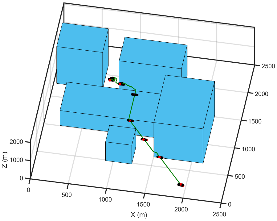
(a) MQS affine transformation

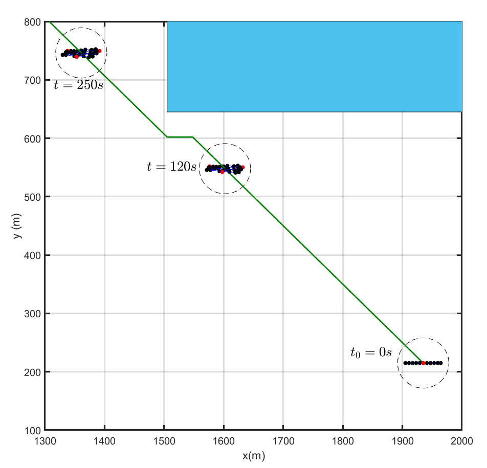
(b) $t=0,120,250s$

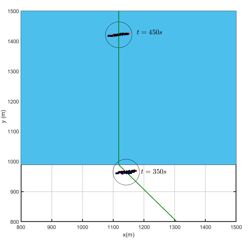
(c) $t=350,450s$

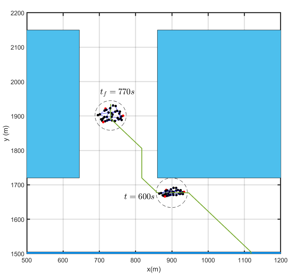
(d) $t=650,770s$

Figure 4: Affine transformation of the MQS in an obstacle-laden environment is illustrated in (a). Top view of MQS formations at sample times (b) $t=0,250,350s$, (c) $t=350,450s$, and (d) $t=650,770s$.

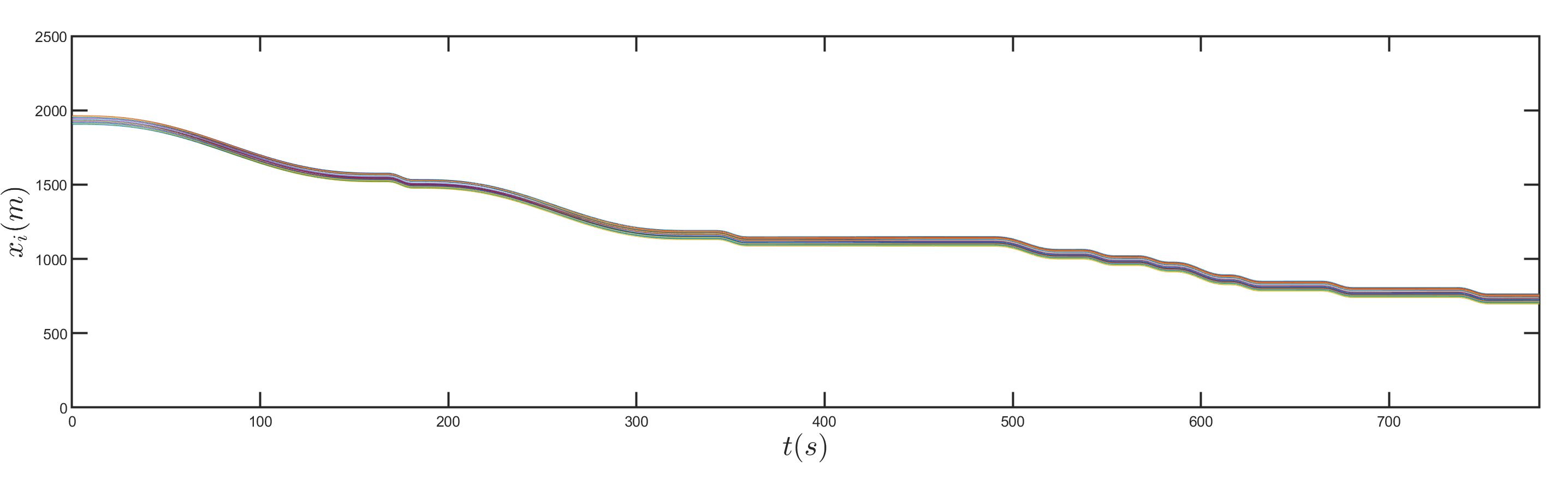
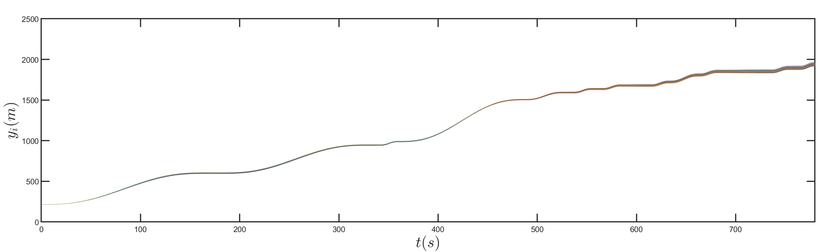
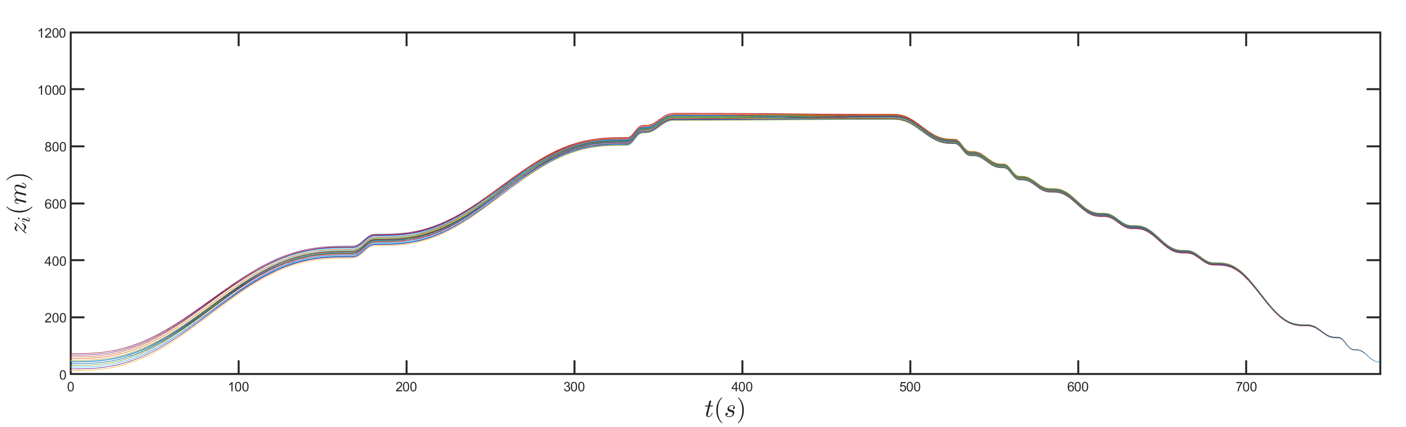
Figure 5: (a,b,c) $x$, $y$, and $z$ components of positions of all agents versus time $t$.

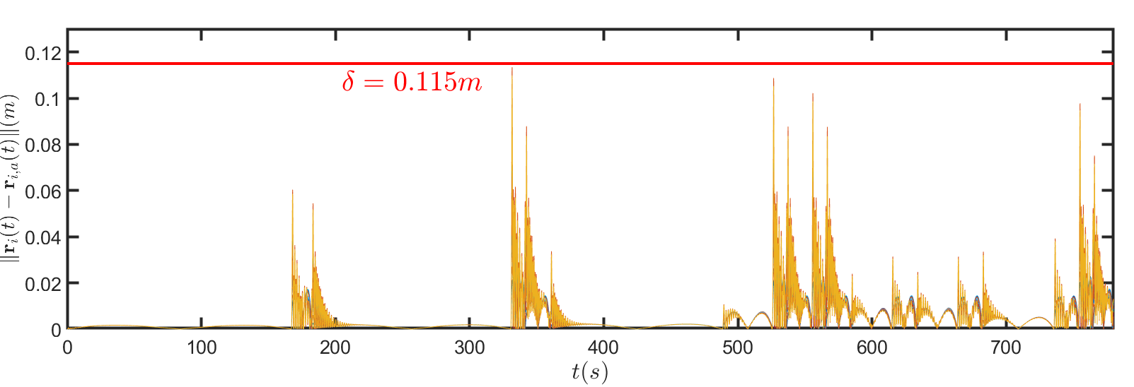
Figure 6: Deviation of agents from global desired trajectories defined by an affine transformation.

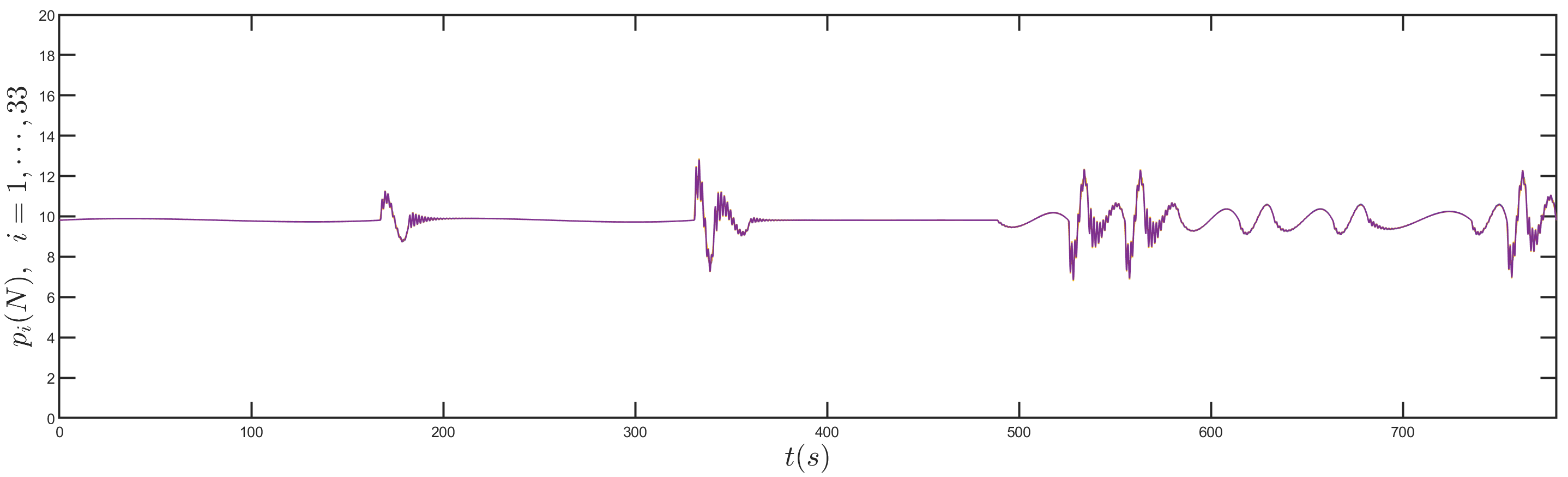
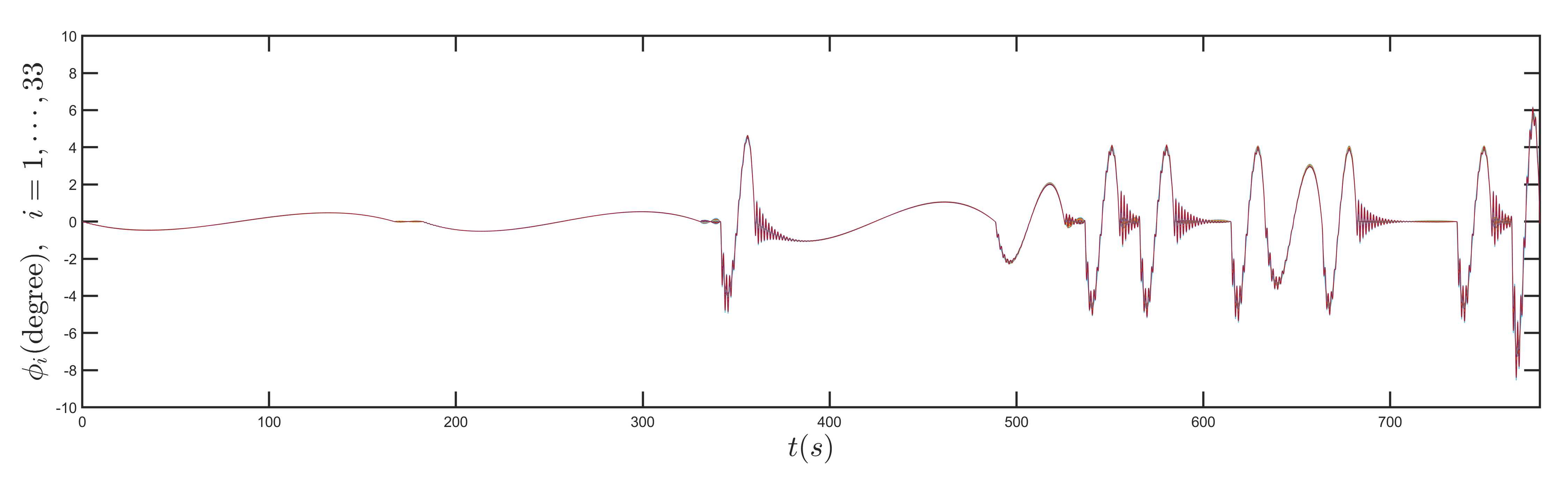
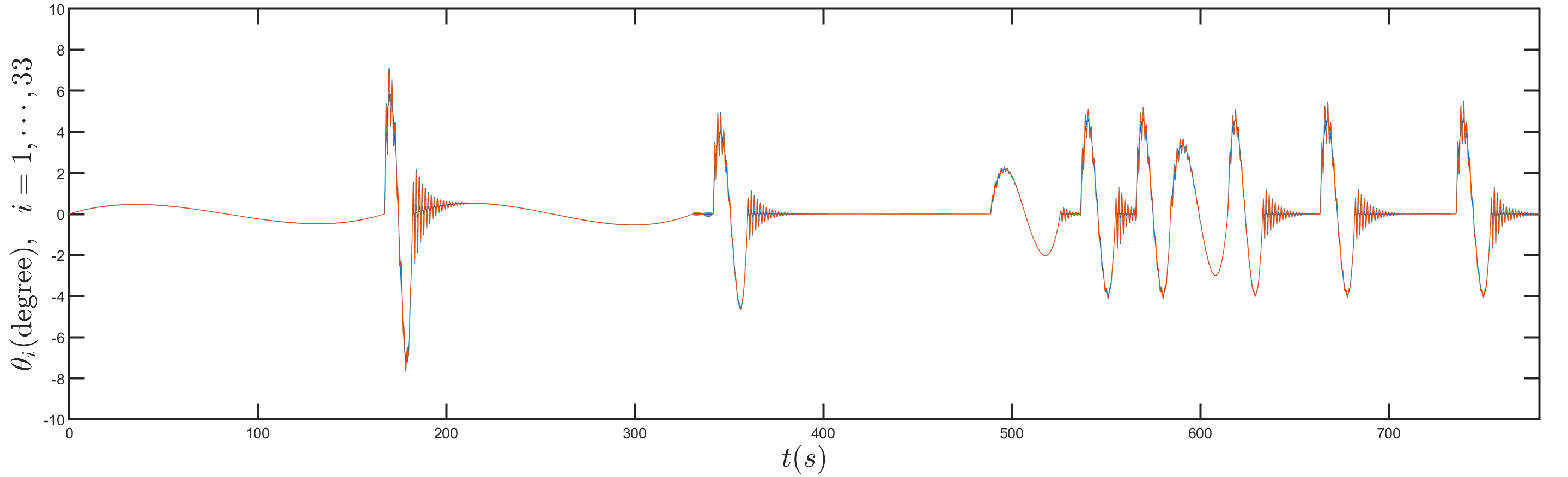
Figure 7: (a,b,c) Thrust force magnitude $p_{i}$, roll angle $\phi_{i}$, and pitch angle $\theta_{i}$ for every quadcopter $i$ versus time.

VII Conclusion

This paper studied the problem of large-scale affine transformation of an MQS in an obstacle-laden environment. By eigen-decomposition of the affine transformation, it was shown how a large-scale collective motion of an MQS can be safely planned such that inter-agent collision avoidance is avoided, quadcopter containment is guaranteed, and no quacopter hits an obstacle in an obstacle-laden environment. Similar to the previously proposed continuum deformation-based coordination approaches our method is scalable to coordination of a large numbers of vehicles, however, it allows to plan more efficient motions due to a more flexible form of the transformation being employed. A comprehensive comparison with other multi-agent coordination approaches proposed in the literature and the development of further calibration/ tuning guidelines is beyond the scope of this paper and is left to future work. Furthermore, the proposed affine transformation-based approach paradigm improves the maneuverability of the swarm coordination by relaxing thee restrictions in the existing continuum deformation coordination approach.

Appendix A Proofs

Proof of Proposition 1: If Assumption 1 and rank condition (3) are satisfied, initial position of quadcopter $i\in\mathcal{V}$ can be expressed by the following linear combination,

$$i\in\mathcal{V},\qquad\mathbf{r}_{i,0}-\mathbf{r}_{1,0}=\sum_{j=2}^{n+1}\alpha_{i,j}\left(\mathbf{r}_{j,0}-\mathbf{r}_{1,0}\right),$$ (74)

where $\alpha_{i,2}$, $\cdots$, $\alpha_{i,n+1}$ are uniquely obtained by

$$\begin{bmatrix}\alpha_{i,2}\\ \vdots\\ \alpha_{i,n+1}\end{bmatrix}=\begin{bmatrix}\mathbf{r}_{2,0}-\mathbf{r}_{1,0}&\cdots&\mathbf{r}_{n+1,0}-\mathbf{r}_{1,0}\end{bmatrix}^{-1}\mathbf{r}_{i,0}.$$ (75)

Now, Eq. (74) can be written in the form of Eq. (4), where $\alpha_{i,1}=1-\sum_{j=2}^{n+1}\alpha_{i,j}$ which in turn implies Eq. (5).

Proof of Proposition 20: Elements of matrix $\mathbf{U}_{D}=\left[U_{ij}\right]\in\mathbb{R}^{3\times 3}$, defined by (18), are expressed as follows:

$$U_{33}=\lambda_{3}C_{\beta_{4}}^{2}C_{\beta_{5}}^{2}+\lambda_{2}C_{\beta_{5}}^{2}S_{\beta_{4}}^{2}+\lambda_{1}S_{\beta_{5}}^{2},$$

$U_{21}=U_{12}$, $U_{32}=U_{23}$, and $U_{31}=U_{13}$. If $\lambda_{1}=\lambda_{2}=\lambda_{3}=\lambda$, then,

$$U_{ij}=\begin{cases}\lambda&i=j\\ 0&i\neq j\end{cases}.$$

Proof of Theorem 1: Inter-agent collision between every two quadcopters is avoided, if

$$\forall i,j\in\mathcal{V},\leavevmode\nobreak\ i\neq j,\qquad\|\mathbf{r}_{i}(t)-\mathbf{r}_{j}(t)\|>2\epsilon.$$ (76)

We can write

$$\left(\mathbf{r}_{i}-\mathbf{r}_{j}\right)=\left(\mathbf{r}_{i,a}-\mathbf{r}_{j,a}\right)-\left(\mathbf{r}_{i,a}-\mathbf{r}_{i}\right)-\left(\mathbf{r}_{j}-\mathbf{r}_{j,a}\right).$$

Therefore,

$$\|\mathbf{r}_{i}-\mathbf{r}_{j}\|\geq\|\mathbf{r}_{i,a}-\mathbf{r}_{j,a}\|-\|\mathbf{r}_{i,a}-\mathbf{r}_{i}\|-\|\mathbf{r}_{j}-\mathbf{r}_{j,a}\|.$$ (77)

Eq. (77) implies that $\|\mathbf{r}_{i}-\mathbf{r}_{j}\|\leq 2\epsilon$, if $\|\mathbf{r}_{i,a}-\mathbf{r}_{i}\|\leq\delta$, $\|\mathbf{r}_{j,a}-\mathbf{r}_{j}\|\leq\delta$, and $\|\mathbf{r}_{i,a}-\mathbf{r}_{j,a}\|\geq 2\left(\epsilon+\delta\right)$. Furthermore, $\|\mathbf{r}_{i,a}-\mathbf{r}_{j,a}\|\geq 2\left(\epsilon+\delta\right)$, if $\|\left(\mathbf{r}_{i,a}-\mathbf{r}_{j,a}\right)\cdot\hat{\mathbf{u}}_{1}\|\geq 2\left(\delta+\epsilon\right)$. Consequently, inter-agent collision avoidance between every two different quadcopters $i$ and $j$ is avoided, if

$$\|\left(\mathbf{r}_{i,a}-\mathbf{r}_{j,a}\right)\cdot\hat{\mathbf{u}}_{1}\|\geq 2\left(\delta+\epsilon\right).$$

Note that

$$\forall i,j\in\mathcal{V},\leavevmode\nobreak\ i\neq j,\qquad\lambda_{1}(t)=\dfrac{|\left(\mathbf{r}_{i,a}(t)-\mathbf{r}_{j,a}(t)\right)\cdot\hat{\mathbf{u}}_{1}(t)|}{|\left(\mathbf{r}_{i,0}(t_{0})-\mathbf{r}_{j,0}(t_{0})\right)\cdot\hat{\mathbf{u}}_{1}(t_{0})|}$$

It is ensured that no quadcopter leaver ball $\bar{\mathcal{S}}(t)$ at any time $t\in[t_{0},t_{f}]$, if

This implies that Eq. (38b) assigns the upper-limit for eigenvalue $\lambda_{1}(t)$ at any time $t\in[t_{0},t_{f}]$. Additionally, It is ensured that no two quadcopters collide, if

$$\forall t\in[t_{0},t_{f}],\qquad\min\limits_{i,j\in\mathcal{V},\leavevmode\nobreak\ i\neq j}\left|\left(\mathbf{r}_{i,a}(t)-\mathbf{r}_{j,a}(t)\right)\cdot\hat{\mathbf{u}}_{1}(t)\right|\geq 2\left(\delta+\epsilon\right).$$

Consequently, Eq. (38a) assigns the lower limit for $\lambda_{1}(t)$ at any time $t\in[t_{0},t_{f}]$.

Because $\mathbf{\Omega}_{0}\subset\mathcal{S}(t_{0})$ and $\mathbf{\Omega}_{0}\subset\mathcal{S}(t_{f})$. Therefore, $\lambda_{2,0}\leq\lambda_{\mathrm{max}}$, $\lambda_{2,f}\leq\lambda_{\mathrm{max}}$, $\lambda_{3,0}\leq\lambda_{\mathrm{max}}$, $\lambda_{3,f}\leq\lambda_{\mathrm{max}}$, and $\lambda_{j}(t)=\lambda_{j,0}\left(1-\gamma(t,T)\right)+\gamma(t,T)\lambda_{j,f}$ remains bounded:

$$j=2,3,\qquad\lambda_{j}(t)\leq\lambda_{\mathrm{max}}$$

at any time $t\in[t_{0},t_{f}]$.

Proof of Theorem 2: If assumptions of Theorem 2 are all satisfied, matrix $\mathbf{G}\in\mathbf{R}^{\left(N-n-1\right)\times\left(N-n-1\right)}$ is non-negative a there exists a directed path between every leader and every follower. By provoking Perron-Frobenius Theorem, it is concluded that the spectral radius of matrix $\mathbf{G}$, denoted by $\rho\left(\mathbf{G}\right)$, is less than $1$ and eigenvalues of matrix $-\mathbf{I}+\mathbf{G}$ are all placed on the left-hand of the $s$-plane inside a disk of radius $\rho\left(\mathbf{G}\right)$ centered at $-1+0\mathrm{j}$. Therefore, matrices $-\mathbf{I}+\mathbf{G}$ and $\mathbf{L}=-\mathbf{I}+\mathbf{W}$ are Hurwitz.

Proof of Theorem 3: Let $\mathbf{R}_{L,0}=\mathrm{vec}\left(\begin{bmatrix}\mathbf{r}_{1,0}&\cdots&\mathbf{r}_{n+1,0}\end{bmatrix}^{T}\right)\in\mathbb{R}^{3\left(n+1\right)\times 1}$ and $\mathbf{R}_{F,0}=\mathrm{vec}\left(\begin{bmatrix}\mathbf{r}_{n+2,0}&\cdots&\mathbf{r}_{N,0}\end{bmatrix}^{T}\right)\in\mathbb{R}^{3\left(N-n-1\right)\times 1},$ define initial position components of leaders and followers, respectively, where $\mathrm{vec}\left(\cdot\right)$ is the matrix vectorization operator. If assumptions of Lemma 3 are satisfied, quadcopters’ initial positions satisfy the following relation:

$$\mathbf{L}\begin{bmatrix}\mathbf{R}_{L,0}\\ \mathbf{R}_{F,0}\end{bmatrix}=\left[\begin{array}[]{cc}-\mathbf{I}&\mathbf{0}\\ \mathbf{F}&\left(-\mathbf{I}+\mathbf{G}\right)\end{array}\right]\begin{bmatrix}\mathbf{R}_{L,0}\\ \mathbf{R}_{F,0}\end{bmatrix}=\begin{bmatrix}-\mathbf{R}_{L,0}\\ \mathbf{0}\end{bmatrix}.$$

Thus,

$$\begin{bmatrix}\mathbf{R}_{L,0}\\ \mathbf{R}_{F,0}\end{bmatrix}=\begin{bmatrix}\mathbf{I}\\ -\left(-\mathbf{I}+\mathbf{G}\right)^{-1}\mathbf{F}\end{bmatrix}\mathbf{R}_{L,0}.$$

Because leaders form an $n$-D simplex at initial time $t_{0}$, positions of every quadcopter $i$ can be uniquely expressed as a linear combination of leaders’ initial positions using relation (4). Therfore,

$$\begin{bmatrix}\mathbf{R}_{L,0}\\ \mathbf{R}_{F,0}\end{bmatrix}=\mathbf{H}\mathbf{R}_{L,0}$$

which in turn implies correctness of Eq. (53a).

Now, we can write

$$\mathbf{Y}_{d}-\mathbf{Y}=\left(\mathbf{I}_{3}\otimes\mathbf{L}\right)\mathbf{Y}+\left(\mathbf{I}_{3}\otimes\mathbf{L}_{0}\right)\mathbf{R}_{L}(t)$$ (78)

On the other hand,

$$\left(\mathbf{I}_{3}\otimes\mathbf{L}\right)\left(\mathbf{Y}-\mathbf{Y}_{a}\right)=\mathbf{Y}_{d}-\mathbf{Y}.$$ (79)

Therefore, Eq. (53b) is proven.
Proof of Theorem 4: Given definition of $\gamma\left(t,T_{l}\right)$ in (27), $\dot{\gamma}\left(t,T_{l}\right)$, $\ddot{\gamma}\left(t,T_{l}\right)$, and $\dddot{\gamma}\left(t,T_{l}\right)$ are decreasing with respect to $T_{l}$. For a given initial time $t_{0}$, $T_{l}$, defined by (25), is increased if $t_{f}$ is increased. Also, $\dot{\gamma}\left(t,T_{l}\right),\ddot{\gamma}\left(t,T_{l}\right),\dddot{\gamma}\left(t,T_{l}\right)\rightarrow 0$, and $\mathbf{V}_{\mathrm{MQS}}\rightarrow\mathbf{0}$, if $T_{f}\rightarrow\infty$. Therefore, there exists a sufficiently-large final time $\tilde{t}_{f}=t_{0}+\tilde{T}_{1}+\cdots+\tilde{T}_{n_{\tau}-1}$ such that the response of zero-initial-state dynamics, given by

$$\begin{bmatrix}\mathbf{E}(t)\\ \dot{\mathbf{E}}(t)\\ \ddot{\mathbf{E}}(t)\\ \dddot{\mathbf{E}}(t)\\ \end{bmatrix}=\mathrm{e}^{\mathbf{A}_{\mathrm{MQS}}{\left(t-t_{0}\right)}}{\color[rgb]{0,0,0}\cancelto{\mathbf{0}}{\begin{bmatrix}\mathbf{E}(t_{0})\\ \dot{\mathbf{E}}(t_{0})\\ \ddot{\mathbf{E}}(t_{0})\\ \dddot{\mathbf{E}}(t_{0})\\ \end{bmatrix}}}+\int_{t_{0}}^{t}\mathrm{e}^{\mathbf{A}_{\mathrm{SYS}}\left(t-\tau\right)}{\mathbf{V}_{\mathrm{MQS}}\left(\tau\right)}\mathrm{d}\tau,$$

ensures that $\|\mathbf{r}_{i}(t)-\mathbf{r}_{i,a}(t)\|<(1-\varrho)\delta$ for every quadcopter $i\in\mathcal{V}$. This also ensures that safety condition (35) is satisfied, if the zero dynamics of the error dynamics (68) ensures that $\|\mathbf{r}_{i}(t)-\mathbf{r}_{i,a}(t)\|<\varrho\delta$ at any time $t\in[t_{0},t_{f}]$.

Appendix B Rotational Kinematics and Dynamics of a Quacopter

We use 3-2-1 standard to determine orientation of quadcopter $i$ at discrete time $k$. Given roll angle $\phi_{i}(t)$, pitch angle $\theta_{i}$, and yaw angle $\psi_{i}$ and the base vectors of the inertial coordinate system ($\hat{\mathbf{e}}_{1}$, $\hat{\mathbf{e}}_{2}$, and $\hat{\mathbf{e}}_{3}$), angular velocity of quadcopter $i\in\mathcal{V}$ is given by

$${\color[rgb]{0,0,0}\bf{\omega}}_{i}=\dot{\psi}_{i}\hat{\mathbf{k}}_{1,i}+\dot{\theta}_{i}\hat{\mathbf{j}}_{2,i}+\dot{\phi}_{i}\hat{\mathbf{i}}_{b,i},$$ (80)

where

$$\begin{bmatrix}\hat{\mathbf{i}}_{1,i}\\ \hat{\mathbf{j}}_{1,i}\\ \hat{\mathbf{k}}_{1,i}\end{bmatrix}=\mathbf{R}\left(0,0,\psi_{i}\right)\begin{bmatrix}\hat{\mathbf{e}}_{1}\\ \hat{\mathbf{e}}_{2}\\ \hat{\mathbf{e}}_{3}\end{bmatrix}=\begin{bmatrix}\cos\psi_{i}&\sin\psi_{i}&0\\ -\sin\psi_{i}&\cos\psi_{i}&0\\ 0&0&1\\ \end{bmatrix}\begin{bmatrix}\hat{\mathbf{e}}_{1}\\ \hat{\mathbf{e}}_{2}\\ \hat{\mathbf{e}}_{3}\end{bmatrix},$$ (81a)

$$\begin{bmatrix}\hat{\mathbf{i}}_{2,i}\\ \hat{\mathbf{j}}_{2,i}\\ \hat{\mathbf{k}}_{2,i}\end{bmatrix}=\mathbf{R}\left(0,\theta_{i},0\right)\begin{bmatrix}\hat{\mathbf{i}}_{1,i}\\ \hat{\mathbf{j}}_{1,i}\\ \hat{\mathbf{k}}_{1,i}\end{bmatrix}=\begin{bmatrix}\cos\theta_{i}&0&-\sin\theta_{i}\\ 0&1&0\\ \sin\theta_{i}&0&\cos\theta_{i}\\ \end{bmatrix}\begin{bmatrix}\hat{\mathbf{i}}_{1,i}\\ \hat{\mathbf{j}}_{1,i}\\ \hat{\mathbf{k}}_{1,i}\end{bmatrix},$$ (81b)

$$\begin{bmatrix}\hat{\mathbf{i}}_{b,i}\\ \hat{\mathbf{j}}_{b,i}\\ \hat{\mathbf{k}}_{b,i}\end{bmatrix}=\mathbf{R}\left(\phi_{i},0,0\right)\begin{bmatrix}\hat{\mathbf{i}}_{2,i}\\ \hat{\mathbf{j}}_{2,i}\\ \hat{\mathbf{k}}_{2,i}\end{bmatrix}=\begin{bmatrix}1&0&0\\ 0&\cos\phi_{i}&\sin\phi_{i}\\ 0&-\sin\phi_{i}&\cos\phi_{i}\end{bmatrix}\begin{bmatrix}\hat{\mathbf{i}}_{2,i}\\ \hat{\mathbf{j}}_{2,i}\\ \hat{\mathbf{k}}_{2,i}\end{bmatrix}.$$ (81c)

Substituting $\hat{\mathbf{e}}_{1}=\left[1\leavevmode\nobreak\ 0\leavevmode\nobreak\ 0\right]^{T}$, $\hat{\mathbf{e}}_{2}=\left[0\leavevmode\nobreak\ 1\leavevmode\nobreak\ 0\right]^{T}$, $\hat{\mathbf{e}}_{3}=\left[0\leavevmode\nobreak\ 0\leavevmode\nobreak\ 1\right]^{T}$, $\hat{\mathbf{i}}_{1,i}$, $\hat{\mathbf{k}}_{1,i}$, $\hat{\mathbf{j}}_{2,i}$, and $\hat{\mathbf{i}}_{b,i}$ into Eq. (80), ${\color[rgb]{0,0,0}\bf{\omega}}_{i}=\left[\omega_{x,i}\leavevmode\nobreak\ \omega_{y,i}\leavevmode\nobreak\ \omega_{z,i}\right]^{T}$ is related by $\dot{\phi}_{i}$, $\dot{\theta}_{i}$, and $\dot{\psi}_{i}$ by

$$\begin{bmatrix}\omega_{x,i}&\omega_{y,i}&\omega_{z,i}\end{bmatrix}^{T}=\mathbf{\Gamma}_{i}\left(\phi_{i},\theta_{i},\psi_{i}\right)\begin{bmatrix}\dot{\phi}_{i}&\dot{\theta}_{i}&\dot{\psi}_{i}\end{bmatrix}^{T},$$ (82)

where

$$\mathbf{\Gamma}_{i}\left(\phi_{i},\theta_{i},\psi_{i}\right)=\begin{bmatrix}1&0&-\sin\theta_{i}\\ 0&\cos\phi_{i}&\cos\theta_{i}\sin\phi_{i}\\ 0&-\sin\phi_{i}&\cos\phi_{i}\cos\theta_{i}\end{bmatrix}.$$ (83)

Angular acceleration of quadcopter $i\in\mathcal{V}$ is obtained by taking the time derivative of the angular velocity vector ${\color[rgb]{0,0,0}\bf{\omega}}_{i}$:

$$\begin{split}\dot{{\color[rgb]{0,0,0}\bf{\omega}}}_{i}=\tilde{\mathbf{B}}_{1,i}\begin{bmatrix}\ddot{\phi}_{i}&\ddot{\theta}_{i}&\ddot{\psi}_{i}\end{bmatrix}^{T}+\tilde{\mathbf{B}}_{2,i}.\end{split}$$ (84)

where

$$\tilde{\mathbf{B}}_{1,i}=\begin{bmatrix}\hat{\mathbf{i}}_{b,i}&\hat{\mathbf{j}}_{2,i}&\hat{\mathbf{k}}_{1,i}\end{bmatrix}$$ (85a)

$$\tilde{\mathbf{B}}_{2,i}=\dot{\theta}_{i}\dot{\psi}_{i}\left(\hat{\mathbf{k}}_{1,i}\times\hat{\mathbf{j}}_{1,i}\right)+\dot{\phi}_{i}\left(\dot{\psi}_{i}\hat{\mathbf{k}}_{1,i}+\dot{\theta}_{i}\hat{\mathbf{j}}_{2,i}\right)\times\hat{\mathbf{i}}_{2,i}$$ (85b)

Note that “$\times$” is the cross product symbol. On the other hand, the rotational dynamics of quadcopter $i$ is given by

$$\dot{\bf{\omega}}_{i}=\mathbf{J}_{i}^{-1}\left(\bf{\omega}_{i}\times\left(\mathbf{J}_{i}\bf{\omega}_{i}\right)+\begin{bmatrix}\tilde{u}_{2,i}&\tilde{u}_{3,i}&\tilde{u}_{4,i}\end{bmatrix}^{T}\right)$$ (86)

where $\tilde{u}_{2,i}=\tau_{\phi,i}$, $\tilde{u}_{3,i}=\tau_{\theta,i}$, $\tilde{u}_{4,i}\tau_{\psi,i}$ (See Eq. (57)). By equating the right-hand sides of Eqs. (84) and (86), we can write

$$\begin{bmatrix}\tilde{u}_{2,i}&\tilde{u}_{3,i}&\tilde{u}_{4,i}\end{bmatrix}^{T}=\mathbf{B}_{1,i}\begin{bmatrix}\ddot{\phi}_{i}&\ddot{\theta}_{i}&\ddot{\psi}_{i}\end{bmatrix}^{T}+\mathbf{B}_{2,i},$$ (87)

where

$$\mathbf{B}_{1,i}=\mathbf{J}_{i}\tilde{\mathbf{B}}_{1,i},$$ (88a)

$$\mathbf{B}_{2,i}=\mathbf{J}_{i}\tilde{\mathbf{B}}_{2,i}-\bf{\omega}_{i}\times\left(\mathbf{J}_{i}\bf{\omega}_{i}\right).$$ (88b)

Appendix C Time Derivatives of the Quadcopter Thrust Force

Let

$$\mathbf{P}_{i}=p_{i}\hat{\mathbf{k}}_{b,i}-m_{i}g\hat{\mathbf{e}}_{1}$$ (89)

be the external force executed on quadcopter $i$. Taking time derivatives from $\mathbf{P}_{i}$, we obtain the following relations:

$$\dot{\mathbf{P}}_{i}=\dot{p}_{i}\hat{\mathbf{k}}_{b,i}+p_{i}{\color[rgb]{0,0,0}\bf{\omega}}_{i}\times\hat{\mathbf{k}}_{b,i},$$ (90a)

$$\ddot{\mathbf{P}}_{i}=\mathbf{O}_{1,i}\mathbf{\Xi}_{i}+\mathbf{O}_{2,i},$$ (90b)

where $\mathbf{\Xi}_{i}=\begin{bmatrix}\ddot{p}_{i}&\ddot{\phi}_{i}&\ddot{\theta}_{i}&\ddot{\psi}_{i}\end{bmatrix}^{T}$,

$$\mathbf{O}_{1,i}=\left[\begin{array}[]{cccc}\hat{\mathbf{k}}_{b,i}&-p_{i}\hat{\mathbf{j}}_{b,i}&p_{i}\left(\hat{\mathbf{j}}_{2,i}\times\hat{\mathbf{k}}_{b,i}\right)&p_{i}\hat{\mathbf{k}}_{1,i}\times\hat{\mathbf{k}}_{b,i}\end{array}\right]\in\mathbb{R}^{3\times 4},$$ (91a)

$$\begin{split}\mathbf{O}_{2,i}=&p_{i}\left[-\dot{\phi}_{i}\dot{\theta}_{i}\left(\hat{\mathbf{k}}_{2,i}\times\hat{\mathbf{k}}_{b,i}\right)+{\color[rgb]{0,0,0}\bf{\omega}}_{i}\times\left({\color[rgb]{0,0,0}\bf{\omega}}_{i}\times\hat{\mathbf{k}}_{b,i}\right)\right]+2\dot{p}_{i}{\color[rgb]{0,0,0}\bf{\omega}}_{i}\times\hat{\mathbf{k}}_{b,i}.\end{split}$$ (91b)

Per Eq. (87), we can write

$$\mathbf{\Xi}_{i}=\mathbf{O}_{3,i}\tilde{\mathbf{u}}_{i}+\mathbf{O}_{4,i},$$ (92)

where $\tilde{\mathbf{u}}_{i}=\begin{bmatrix}\tilde{u}_{1,i}&\cdots&\tilde{u}_{4,i}\end{bmatrix}^{T}=\begin{bmatrix}\ddot{p}_{i}&\tau_{\phi,i}&\tau_{\theta,i}&\tau_{\psi,i}\end{bmatrix}^{T}$,

$$\mathbf{O}_{3,i}=\left[\begin{array}[]{c|c}1&\mathbf{0}_{1\times 3}\\ \hline\cr\mathbf{0}_{3\times 1}&\mathbf{B}_{1,i}^{-1}\end{array}\right],$$

$$\mathbf{O}_{4,i}=\left[\begin{array}[]{c}0\\ \hline\cr-\mathbf{B}_{1,i}^{-1}\mathbf{B}_{2,i}\end{array}\right].$$

By substituting (92), Eq. (90b) is converted to

$$\ddot{\mathbf{P}}_{i}=\mathbf{O}_{1,i}\mathbf{O}_{3,i}\tilde{\mathbf{u}}_{i}+\mathbf{O}_{1,i}\mathbf{O}_{4,i}+\mathbf{O}_{2,i}.$$ (93)

Note that $\mathbf{s}_{i}={1\over m_{i}}\ddot{\mathbf{P}}_{i}$ where $\mathbf{s}_{i}$ is the input vector of the external dynamics of quadcopter $i$ (see Section V-B).

Hossein Rastgoftar an Assistant Professor at Villanova University and an Adjunct Assistant Professor at the University of Michigan. He was an Assistant Research Scientist in the Aerospace Engineering Department from 2017 to 2020. Prior to that he was a postdoctoral researcher at the University of Michigan from 2015 to 2017. He received the B.Sc. degree in mechanical engineering-thermo-fluids from Shiraz University, Shiraz, Iran, the M.S. degrees in mechanical systems and solid mechanics from Shiraz University and the University of Central Florida, Orlando, FL, USA, and the Ph.D. degree in mechanical engineering from Drexel University, Philadelphia, in 2015.

Ilya V. Kolmanovsky received M.S. and Ph.D. degrees in aerospace engineering and the M.A. degree in mathematics from the University of Michigan, Ann Arbor, MI, USA, in 1993, 1995, and 1995, respectively. Between 1995 and 2009, he was with Ford Research and Advanced Engineering, Dearborn, MI, USA. He is currently a Full Professor with the Department of Aerospace Engineering, University of Michigan. His research interests include control theory for systems with state and control constraints, and control applications to aerospace and automotive systems. Dr. Kolmanovsky was a recipient of the Donald P. Eckman Award of American Automatic Control Council and two IEEE Transactions on Control Systems Technology Outstanding Paper Awards. Dr. Kolmanovsky is an IEEE Fellow and AIAA Associate Fellow.

References

• [1] M.ย K. Allouche and A.ย Boukhtouta, โ€œMulti-agent coordination by temporal plan fusion: Application to combat search and rescue,โ€ Information Fusion, vol.ย 11, no.ย 3, pp. 220โ€“232, 2010.
• [2] A.ย Kleiner, A.ย Farinelli, S.ย Ramchurn, B.ย Shi, F.ย Maffioletti, and R.ย Reffato, โ€œRmasbench: benchmarking dynamic multi-agent coordination in urban search and rescue,โ€ in 12th International Conference on Autonomous Agents and Multiagent Systems (AAMAS 2013), 2013, pp. 1195โ€“1196.
• [3] O.ย Ali, B.ย Saintย Germain, J.ย Vanย Belle, P.ย Valckenaers, H.ย Vanย Brussel, and J.ย Vanย Noten, โ€œMulti-agent coordination and control system for multi-vehicle agricultural operations.โ€ in AAMAS, 2010, pp. 1621โ€“1622.
• [4] S.ย Yuan, X.ย Lai, X.ย Zhao, X.ย Xu, and L.ย Zhang, โ€œDistributed structural health monitoring system based on smart wireless sensor and multi-agent technology,โ€ Smart Materials and Structures, vol.ย 15, no.ย 1, p.ย 1, 2005.
• [5] H.ย Idris, K.ย Bilimoria, D.ย Wing, S.ย Harrison, and B.ย Baxley, โ€œAir traffic management technology demonstrationโ€“3 (atd-3) multi-agent air/ground integrated coordination (maagic) concept of operations,โ€ NASA/TM-2018-219931, NASA, Washington DC, Tech. Rep., 2018.
• [6] J.ย Qin, C.ย Yu, and B.ย D. Anderson, โ€œOn leaderless and leader-following consensus for interacting clusters of second-order multi-agent systems,โ€ Automatica, vol.ย 74, pp. 214โ€“221, 2016.
• [7] C.ย Ding, X.ย Dong, C.ย Shi, Y.ย Chen, and Z.ย Liu, โ€œLeaderless output consensus of multi-agent systems with distinct relative degrees under switching directed topologies,โ€ IET Control Theory & Applications, vol.ย 13, no.ย 3, pp. 313โ€“320, 2018.
• [8] Y.ย Wu, Z.ย Wang, S.ย Ding, and H.ย Zhang, โ€œLeaderโ€“follower consensus of multi-agent systems in directed networks with actuator faults,โ€ Neurocomputing, vol. 275, pp. 1177โ€“1185, 2018.
• [9] H.ย Wang, W.ย Yu, G.ย Wen, and G.ย Chen, โ€œFixed-time consensus of nonlinear multi-agent systems with general directed topologies,โ€ IEEE Transactions on Circuits and Systems II: Express Briefs, vol.ย 66, no.ย 9, pp. 1587โ€“1591, 2018.
• [10] G.ย Wen, J.ย Huang, C.ย Wang, Z.ย Chen, and Z.ย Peng, โ€œGroup consensus control for heterogeneous multi-agent systems with fixed and switching topologies,โ€ International Journal of Control, vol.ย 89, no.ย 2, pp. 259โ€“269, 2016.
• [11] J.ย Zhou, C.ย Sang, X.ย Li, M.ย Fang, and Z.ย Wang, โ€œH-infinity consensus for nonlinear stochastic multi-agent systems with time delay,โ€ Applied Mathematics and Computation, vol. 325, pp. 41โ€“58, 2018.
• [12] X.ย Zhang, Y.ย Huang, L.ย Li, Y.ย Wang, and W.ย Duan, โ€œDelay-dependent stability analysis of modular microgrid with distributed battery power and soc consensus tracking,โ€ IEEE Access, vol.ย 7, pp. 101โ€‰125โ€“101โ€‰138, 2019.
• [13] H.ย Du, G.ย Wen, D.ย Wu, Y.ย Cheng, and J.ย Lรผ, โ€œDistributed fixed-time consensus for nonlinear heterogeneous multi-agent systems,โ€ Automatica, vol. 113, p. 108797, 2020.
• [14] D.ย Xu, X.ย Wang, Y.ย Hong, and Z.-P. Jiang, โ€œGlobal robust distributed output consensus of multi-agent nonlinear systems: An internal model approach,โ€ Systems & Control Letters, vol.ย 87, pp. 64โ€“69, 2016.
• [15] Y.ย Cao, W.ย Ren, and M.ย Egerstedt, โ€œDistributed containment control with multiple stationary or dynamic leaders in fixed and switching directed networks,โ€ Automatica, vol.ย 48, no.ย 8, pp. 1586โ€“1597, 2012.
• [16] M.ย Ji, G.ย Ferrari-Trecate, M.ย Egerstedt, and A.ย Buffa, โ€œContainment control in mobile networks,โ€ IEEE Transactions on Automatic Control, vol.ย 53, no.ย 8, pp. 1972โ€“1975, 2008.
• [17] G.ย Notarstefano, M.ย Egerstedt, and M.ย Haque, โ€œContainment in leaderโ€“follower networks with switching communication topologies,โ€ Automatica, vol.ย 47, no.ย 5, pp. 1035โ€“1040, 2011.
• [18] W.ย Li, L.ย Xie, and J.-F. Zhang, โ€œContainment control of leader-following multi-agent systems with markovian switching network topologies and measurement noises,โ€ Automatica, vol.ย 51, pp. 263โ€“267, 2015.
• [19] J.ย Shen and J.ย Lam, โ€œContainment control of multi-agent systems with unbounded communication delays,โ€ International Journal of Systems Science, vol.ย 47, no.ย 9, pp. 2048โ€“2057, 2016.
• [20] K.ย Liu, G.ย Xie, and L.ย Wang, โ€œContainment control for second-order multi-agent systems with time-varying delays,โ€ Systems & Control Letters, vol.ย 67, pp. 24โ€“31, 2014.
• [21] X.ย Wang, S.ย Li, and P.ย Shi, โ€œDistributed finite-time containment control for double-integrator multiagent systems,โ€ IEEE Transactions on Cybernetics, vol.ย 44, no.ย 9, pp. 1518โ€“1528, 2013.
• [22] H.ย Liu, L.ย Cheng, M.ย Tan, Z.ย Hou, and Y.ย Wang, โ€œDistributed exponential finite-time coordination of multi-agent systems: containment control and consensus,โ€ International Journal of Control, vol.ย 88, no.ย 2, pp. 237โ€“247, 2015.
• [23] H.ย Rastgoftar, Continuum deformation of multi-agent systems.ย ย ย Springer, 2016.
• [24] H.ย Rastgoftar, E.ย M. Atkins, and D.ย Panagou, โ€œSafe multiquadcopter system continuum deformation over moving frames,โ€ IEEE Transactions on Control of Network Systems, vol.ย 6, no.ย 2, pp. 737โ€“749, 2018.
• [25] H.ย Rastgoftar and E.ย M. Atkins, โ€œSafe multi-cluster uav continuum deformation coordination,โ€ Aerospace Science and Technology, vol.ย 91, pp. 640โ€“655, 2019.
• [26] R.ย Miranda-Colorado, โ€œParameter identification of conservative hamiltonian systems using first integrals,โ€ Applied Mathematics and Computation, vol. 369, p. 124860, 2020.