TEOBResumS: assessment of consistent next-to-quasicircular corrections and post-adiabatic approximation in multipolar binary black holes waveforms

Abstract

The use of effective-one-body (EOB) waveforms for black hole binaries analysis in gravitational-wave astronomy requires faithful models and fast generation times. A key aspect to achieve faithfulness is the inclusion of numerical-relativity (NR) informed next-to-quasicircular corrections (NQC), dependent on the radial momentum, to the waveform and radiation reaction. A robust method to speed up the waveform generation is the post-adiabatic iteration to approximate the solution of the EOB Hamiltonian equations. In this work, we assess the performances of a fast NQC prescription in combination to the post-adiabatic method for generating multipolar gravitational waves. The outlined approach allows a consistent treatment of NQC in both the waveform and the radiation-reaction, does not require iterative procedures to achieve high faithfulness, and can be efficiently employed for parameter estimation. Comparing to 611 NR simulations, for total mass $10M_{\odot}\leq M\leq 200M_{\odot}$ and using the Advanced LIGO noise, the model has EOB/NR unfaithfulness well below $0.01$, with 78.5% of the cases below $0.001$. We apply the model to the parameter estimation of GW150914 exploring the impact of the new NQC and of the higher modes up to $\ell=m=8$.

I Introduction

The continuously increasing sensitivity of gravitational-wave (GW) detectors Acernese et al. (2015); Aasi et al. (2015) and the associated compact binaries detections Abbott et al. (2020) motivate work towards physically complete, precise and efficient gravitational-wave models. The effective-one-body (EOB) framework Buonanno and Damour (1999, 2000); Damour et al. (2000); Damour (2001); Damour et al. (2015) is a possible approach to the general-relativistic two-body problem that, by construction, allows the inclusion of perturbative (post-Newtonian, black hole perturbations) and full numerical relativity (NR) results. It currently represents a state-of-art approach for modeling waveforms from binary black holes, conceptually designed to describe the entire inspiral-merger-ringdown phenomenology of quasicircular binaries Nagar and Rettegno (2019); Nagar et al. (2018); Cotesta et al. (2018); Nagar et al. (2019a, 2020); Ossokine et al. (2020); Schmidt et al. (2021) or even eccentric inspirals Nagar et al. (2021a) and hyperbolic captures Nagar et al. (2021b, a). In the low-frequency inspiral regime, where NR simulations are not available, EOB it is the only alternative to improve standard and badly convergent post-Newtonian (PN) models for exploring systematics effects in the modeling of the radiation reaction Gamba et al. (2020a). In the high-frequency merger regime, EOB can generate highly faithful waveforms for GW astronomy thank to the inclusion of NR information Nagar et al. (2019a, 2020). This paper focuses on a key aspect for EOB models: the consistent and efficient inclusion of NR information in the multipolar waveform.

Current EOB models are informed by NR in two separate ways: (i) on the one hand, through EOB flexibility parameters Damour et al. (2002) that allow to improve the conservative part of the dynamics, i.e. typically as effective high-order terms in the orbital, spin-orbit or spin-spin part sector of the EOB Hamiltonian; (ii) on the other hand, through next-to-quasi-circular (NQC) corrections to the multipolar waveform (and flux) Damour and Nagar (2007); Damour et al. (2008a, b); Damour and Nagar (2009). The latter enter as multiplicative factors, that depend on the radial motion, and correct the EOB factorized quasicircular waveform Damour et al. (2009); Messina et al. (2018) multipole by multipole, so to introduce effective, NR-tuned, modifications to both the amplitude and the phase. NQC corrections are essential to improve the analytical quasicircular waveform during the late plunge up to merger; they also guarantee a smooth transition to the subsequent ringdown phase. Importantly, NQC parameters are the largest set of data inferred from NR. For example, the spin-aligned TEOBResumS model uses NR information to determine 2 parameters (one orbital and one spin-orbital)Nagar et al. (2020) for the spin-aligned effective 5PN Hamiltonian, but 36 parameters (two for amplitude and two for phase) for the NQC-corrected multipolar waveform, that can have up to 9 multipoles completed through merger and ringdown Nagar et al. (2020): $(\ell,|m|)=\{(2,2),(2,1),(3,3),(3,2),(3,1),(4,4),(4,3),(4,2),(5,5)\}$. All higher modes up to $\ell=8$ can also be optionally generated by the model, although currently without the NR-informed merger ringdown Nagar et al. (2019a). In the spin-aligned SEOBNRv4 Bohé et al. (2017) and SEOBNRv4_HM Cotesta et al. (2018) the amount of information inferred from NR is similar, although it is included differently. In particular: (i) there are 3 flexibility parameters entering the Hamiltonian Bohé et al. (2017) (that is different from the TEOBResumS one Rettegno et al. (2019)); (ii) for each waveform multipole there are 5 NQC parameters (3 for the amplitude and 2 for the phase), for a total of 25 parameters since the modes completed through merger and ringdown are $(\ell,|m|)=\{(2,2),(2,1),(3,3),(4,4),(5,5)\}$. In addition, SEOBNRv4_HM needs two more effective corrections to the $(2,1)$ and $(5,5)$ amplitudes that are calibrated to NR.

To achieve internal consistency between the waveform and the radiation reaction in the EOB equations of motion, the NQC amplitude factor should be also incorporated within the radiation reaction force, i.e. the flux of mechanical angular momentum. A possible approach to this problem is to iterate the dynamics several time, updating the values of NQC parameters at each step, until their values are seen to converge Damour and Nagar (2009); Damour et al. (2013). This procedure, though necessary from the physical point of view, cannot be part of a waveform generator for parameter estimation, as it would increase the global computational time at least by a factor four. Yet, it is important because, as we will see below, it also yields a fractional agreement between the NR and EOB angular momentum flux $\lesssim 1\%$ even during the late-inspiral and plunge regime. One way out is simply to avoid this iterative procedure and keep radiation reaction without the NQC corrective factor. This route is the one implemented in SEOBNRv4 Bohé et al. (2017), but evidently the model lacks of self consistency between radiation reaction and waveform.

Reference Nagar et al. (2020) (hereafter Paper I), shows that the $(2,2)$ mode of TEOBResumS with iterated NQC corrections achieves an overall EOB/NR unfaithfulness for total mass $10M_{\odot}\leq M\leq 200M_{\odot}$ is always below $0.5\%$, with one single outlier grazing the $0.85\%$ level. SEOBNRv4, without the iterated NQC at most grazes $1\%$, although it has been tested on only 114 spin-aligned NR waveforms Bohé et al. (2017) up to $q=10$. This number is six time smaller than the testing sample of TEOBResumS, that is also pushed up to mass ratio $q=18$.

In this paper, we describe the NQC fitting procedure used in TEOBResumS in order to obtain a consistent (waveform and flux) NQC term without the iteration procedure. This NQC treatment is the default option in the most recent version of TEOBResumS, that incorporates higher modes Nagar et al. (2020) and has been already used in Breschi et al. (2021), although not reported before. For simplicity we will refer to this version as v2. By contrast, the v1 tag refers to the first implementation of TEOBResumS Nagar et al. (2018). We also present an updated faithfulness assessment of the TEOBResumS $\ell=m=2$ waveform against a large set of NR simulations where we include for the first time: (i) the new NQC fits; (ii) the (iterated) post-adiabatic approximation to the dynamics Damour et al. (2013); Nagar and Rettegno (2019); Nagar et al. (2019b); Rettegno et al. (2019).

The post-adiabatic (PA) approximation is a robust method to solve the EOB Hamiltonian equations by an iterative analytical procedure rather than solving numerically the set of ODEs. The PA was shown to be crucial for parameter estimation with TEOBResumS, both for black holes and neutron stars Gamba et al. (2020a, b); Breschi et al. (2021). In particular, the PA is a simple, flexible and robust alternative to surrogate methods Lackey et al. (2017); Cotesta et al. (2020). By using this approach, the dynamics computation can become up to 20 times faster and its employment is among the reasons why the TEOBResumS computational cost is generally one order of magnitude smaller than the SEOBNRv4HM Cotesta et al. (2018) one. This method is implemented in the most recent stand-alone release of TEOBResumS as well as in the v1 release within the LIGO Algorithm Library (LAL) LIGO Scientific Collaboration (2018a). We demonstrate the use of the NQC fits and of the PA approximation in parameter estimation on GW150914, notably using the multipolar waveform with all modes up to $\ell=m=8$. In particular, the possibility of doing PE with and without NQC fits allows us to analyze in detail a very specific source of analytical systematics in waveform modeling.

This paper is organized as follows. Section II reviews the motivations and structure of the NQC correction and the new fits. Sec. III discusses the validation of the production setup of TEOBResumS with the new NQCs and the PA against 595 SXS and 19 BAM waveforms. In Sec. IV we give an account of the TEOBResumS waveform generation time. Finally, Sec. V presents the application to GW150914 analysis. After the conclusions, the paper has two appendices: Appendix A reports the unfaithfulness plots of Paper I to facilitate the comparison with the new results; Appendix B contains all the details on the new NQC fits.

II EOB Next-to-quasicircular corrections

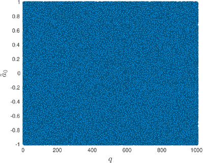
Figure 1: Robustness of the TEOBResumS implementation with higher modes, PA dynamics and NQC corrections fits in the flux. Waveforms (blue markers) are generated with no failures for 250,000 binaries with parameters uniformly sampled at random in the ranges $1\leq q\leq 1000$ and $-1<\chi_{i}<1$. The spin parameter on the $y$-axis is defined as $\tilde{a}_{0}=\chi_{\rm eff}=(m_{1}\chi_{1}+m_{2}\chi_{2})/M$.

Next-to-quasi-circular corrections were introduced in the first EOB analysis of the transition from inspiral to plunge, merger and ringdown in the test-particle limit Damour and Nagar (2007). They were originally conceived as an effective noncircular correction to the flux of mechanical angular momentum $\cal{F}_{\varphi}$, so to consistently model it during the plunge up to merger (see Fig. 2 in Ref. Damour and Nagar (2007)). In subsequent EOB/NR works Damour et al. (2008a, b) they were moved to the $(2,2)$ waveform in order to achieve an optimal EOB/NR amplitude and phase agreement at merger and ease the attachment of the ringdown part. Finally, Ref. Damour and Nagar (2009) introduced the current paradigm, within TEOBResumS, of having them in both the $(2,2)$ waveform and radiation reaction, with the iterative procedure to consistently determine the effective NQC parameters entering the $(2,2)$ amplitude. More precisely, each factorized and resummed Damour et al. (2009) EOB waveform mode $(\ell,m)$ is dressed by a multiplicative contribution $\hat{h}^{\rm NQC}_{\ell m}$ as

$$h_{\ell m}=h_{\ell m}^{(N,\epsilon)}\hat{h}_{\ell m}\hat{h}^{\rm NQC}_{\ell m}\ ,$$ (1)

where $h_{\ell m}^{(N,\epsilon)}$ is the Newtonian prefactor with parity $\epsilon$ and $\hat{h}_{\ell m}$ the relativistic correction. The NQC factor is parametrized by four parameters $(a^{\ell m}_{1},a^{\ell m}_{2},b^{\ell m}_{1},b^{\ell m}_{2})$,

$$\hat{h}^{\rm NQC}_{\ell m} =\left(1+a_{1}^{(\ell,m)}n^{(\ell,m)}_{1}+a_{2}^{(\ell,m)}n^{(\ell,m)}_{2}\right)$$

$$\times e^{{\rm i}(b_{1}^{(\ell,m)}n^{(\ell,m)}_{3}+b_{2}^{(\ell,m)}n^{(\ell,m)}_{4})}\ ,$$ (2)

where $n_{i}^{(\ell,m)}$ are functions depending on the radial velocity and acceleration, see Eqs.(3.32)-(3.35) of Nagar et al. (2019a) and Ref. Damour et al. (2013). Parameters $(a^{(\ell,m)}_{1},a^{(\ell,m)}_{2})$ determine the NQC of the amplitude’s multipole $(\ell,m)$, while $(b^{(\ell,m)}_{1},b^{(\ell,m)}_{2})$ determine the NQC to the phase and frequency of the multipole $(\ell,m)$. The parameters $(a^{(2,2)}_{1},a^{(2,2)}_{2})$ play a special role as they are those also included in the radiation reaction Damour and Nagar (2009). Their best values are determined by an iterative procedure, e.g. the one of Paper I. The parameters $(a^{(\ell,m)}_{1},a^{(\ell,m)}_{2},b^{(\ell,m)}_{1},b^{(\ell,m)}_{2})$ with $(\ell,m)\neq(2,2)$ are instead best generated by solving a set of four coupled algebraic equations and imposing NR-informed fits of amplitude, frequency and their first derivatives around merger Damour and Nagar (2009); Damour et al. (2013); Nagar et al. (2017, 2018, 2019a, 2020).

II.1 Fitting NQC parameters $(a^{(2,2)}_{1},a^{(2,2)}_{2})$

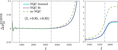
Figure 2: Comparison between EOB/NR phase differences $\Delta\phi_{22}^{\rm EOBNR}\equiv\phi_{22}^{\rm EOB}-\phi_{22}^{\rm NR}$ for dataset SXS:BBH:0257, configuration $(q,\chi_{1},\chi_{2})=(2,+0.85,+0.85)$. Waves are aligned in the early inspiral, on the time interval indicated by the vertical dash-dotted lines in the left panel. The vertical line in the right panel marks merger time, corresponding to the peak of the $\ell=m=2$ amplitude. The curves correspond to: (i) iterated NQC parameters $(a_{1}^{(2,2)},a_{2}^{(2,2)})$ in radiation reaction as in Paper I; fitted NQC parameters; no NQC parameters in radiation reaction. The corresponding maximum values of the EOB/NR unfaithfulness $\bar{F}$ from Eq. (5) are $0.414\%$, $0.456\%$ and $1.7\%$ respectively. See the corresponding $\bar{F}(M)$ curves in Figs. 4 and 11 below.

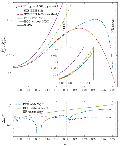
Figure 3: EOB/NR comparison of the fluxes of angular momentum at infinity for a demonstrative configuration $(q,\chi_{1},\chi_{2})=(6.281,0.009,-0.8)$ corresponding to SXS:BBH:1436 dataset. Top panel: Newton-normalized fluxes versus PN frequency parameter $x$. Bottom panel: EOB/NR fractional differences. The (iterated) EOB flux with the NQC correction factor shows $\sim 10^{-3}$ fractional agreement with the NR flux up to the EOB last stable orbit. A much larger difference is found in the absence of NQC correction factor. The Taylor-expanded 3.5PN flux is also shown to highlight the power of the EOB resummation procedures. See text for details.

The high NR-faithfulness of TEOBResumS in Paper I depends on the EOB flexibility functions $(a_{6}^{c},c_{3})$ that are NR-informed under the conditions that $(a^{(2,2)}_{1},a^{(2,2)}_{2})$ are determined from the iterative procedure. Dropping this would imply a worsening of the global EOB/NR agreement (see below). As a consequence, we need to construct accurate fits of $(a^{(2,2)}_{1},a^{(2,2)}_{2})$ all over the parameter space so to obtain EOB/NR unfaithfulness similar to the iterative procedure while not requiring iterations. To do so, we proceed as follows. First, the parameters $(a^{(2,2)}_{1},a^{(2,2)}_{2})$ are determined with the same iterative procedure of Paper I for $2291$ simulations up to mass-ratio of $q=30$ with aligned spins up to $\chi_{1}=\chi_{2}=\pm 0.99$. Second, the values $(a^{(2,2)}_{1},a^{(2,2)}_{2})$ are fitted across the parameter space. The latter is divided in four different regions:

1. Nonspinning sector, $\chi_{1}=\chi_{2}=0$

2. Spinning sector, equal-mass sector with $\nu>0.2485$

3. Spinning sector, $0.16\leq\nu<0.2485$

4. Spinning sector, with $\nu\leq 0.16$.

In each region different templates are employed to better capture the functional behavior of $(a^{(2,2)}_{1},a^{(2,2)}_{2})$. All fits are done using as single spin parameter the standard spin combination

$$\hat{S}\equiv\dfrac{S_{1}+S_{2}}{M^{2}}=X_{1}^{2}\chi_{1}+X_{2}^{2}\chi_{2}\ ,$$ (3)

where $S_{i}$ are the dimensionful individual spins, $\chi_{i}\equiv S_{i}/m_{i}^{2}$ are the dimensionless spins and $X_{i}\equiv m_{i}/M$. The spin parameter $\hat{S}$ is actually used in the fits only for the equal-mass case. In the other situations, it looks more flexible to incorporate some $\nu$-dependence and use instead

$$\hat{S}_{\nu}\equiv\dfrac{\hat{S}}{1-2\nu}\ .$$ (4)

All the details of the fitting procedure are in Appendix B.

Our NQC implementation has been extensively tested to check its robustness all over the parameter space. Fig. 1 illustrates that the new NQC implementation never failed for 420,000 binary configurations drawn from random distributions of spins $-1<\tilde{a}_{0}<+1$ and mass ratios $1\leq q\leq 1000$. The EOB runs in the figure are generated with the PA method, computing the dynamics up to the dimensionless radius $r=R/GM=14$ on a grid with $dr=0.1$ using the 8th PA order Nagar and Rettegno (2019). The other NR-informed EOB parameters are the same as in Nagar et al. (2020) and corresponds to the default configuration of TEOBResumS for parameter estimation.

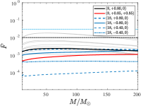
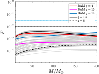
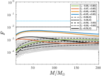
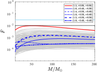
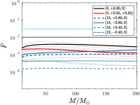
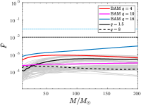
Figure 4: EOB/NR unfaithfulness for the $\ell=m=2$ mode using all currently available spin-aligned SXS NR simulations and a bunch of BAM simulations. Top row: TEOBResumS with the PA approximation for the inspiral and without NQC corrections in radiation reaction. Bottom row: TEOBResumS with the PA approximation for the inspiral and with the NQC parameters obtained by the fit in radiation reaction. From left to right, the columns use the following NR data: SXS spin-aligned waveforms publicly released before February 3, 2019; SXS spin-aligned waveforms publicly released after February 3, 2019; spin-aligned BAM data; nonspinning configurations. The quality of the EOB performance with the NQC fits is very good and essentially equivalent to the outcome of the exact iterative procedure of Ref. Nagar et al. (2020), that is reported in Fig. 11 in Appendix for completeness.

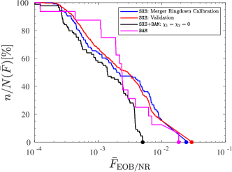
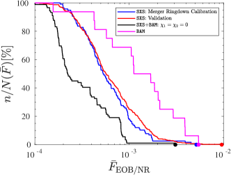
Figure 5: Summary histogram of EOB/NR unfaithfulness $\bar{F}_{\rm EOB/NR}$ over the full NR database of 611 simulations, without NQC fits (top panel) and with fits (bottom panel). The various SXS subsets, nonspinning (black online, 89 waveforms), merger-ringdown calibration (blue online, 116 spin-aligned waveforms) and validation (red online, 388 spin-aligned waveform) as defined in Paper I are presented separately. The plot shows the fraction (expressed in $\%$) $n/N_{\rm set}$, where $N_{\rm set}$ is the total number of waveforms in a given NR-waveform set and $n$ is the number of waveforms, in the same set, that, given a value $\bar{F}$, have $\bar{F}^{\rm max}_{\rm EOB/NR}\geq\bar{F}$. The colored marker highlight the largest values in each NR dataset.

Table 1: GW190514 analysis and main parameters intervals. We report the median and $90\%$ credible region for the parameters extracted from the posterior distribution. Explicitly, the total mass $M$, the chirp mass $\mathcal{M_{\rm c}}$, the individual masses $m_{i}$, the mass ratio $q$, the dimensionless spins $\chi_{i}\equiv S_{i}/m_{i}^{2}$ and their combination $\chi_{\rm eff}=\tilde{a}_{0}=(m_{1}\chi_{1}+m_{2}\chi_{2})/M$, the luminosity distance $D_{\rm L}$, the inclination angle $\iota$, the right ascension $\alpha$ and declination $\delta$. In the last row, we show the logarithmic Bayes’ factor with its standard deviation.

	22+NQCfit	22+noNQCfit	LM+NQCfit	LM+noNQCfit	HM+NQCfit	HM+noNQCfit
$M~{}{\rm[M_{\odot}]}$	$72.11_{-2.55}^{+2.79}$	$73.42_{-2.67}^{+2.88}$	$72.48_{-2.31}^{+3.51}$	$72.87_{-2.85}^{+3.66}$	$73.30_{-2.74}^{+3.18}$	$72.86_{-2.88}^{+3.31}$
$\mathcal{M}_{\rm c}~{}{\rm[M_{\odot}]}$	$31.16_{-1.20}^{+1.25}$	$31.72_{-1.31}^{+1.30}$	$31.39_{-1.12}^{+1.50}$	$31.54_{-1.26}^{+1.59}$	$31.75_{-1.26}^{+1.42}$	$31.54_{-1.25}^{+1.46}$
$m_{1}~{}{\rm[M_{\odot}]}$	$39.67_{-3.32}^{+4.31}$	$40.06_{-3.07}^{+3.79}$	$38.83_{-2.35}^{+3.73}$	$39.63_{-2.97}^{+4.66}$	$39.31_{-2.68}^{+4.72}$	$39.06_{-2.63}^{+4.46}$
$m_{2}~{}{\rm[M_{\odot}]}$	$32.53_{-3.77}^{+3.37}$	$33.34_{-4.04}^{+3.06}$	$33.66_{-3.82}^{+2.86}$	$33.25_{-3.46}^{+3.10}$	$33.83_{-3.88}^{+3.06}$	$33.68_{-3.68}^{+2.90}$
$q$	$1.22_{-0.19}^{+0.29}$	$1.20_{-0.17}^{+0.27}$	$1.15_{-0.13}^{+0.26}$	$1.19_{-0.16}^{+0.26}$	$1.16_{-0.14}^{+0.28}$	$1.16_{-0.14}^{+0.27}$
$\chi_{1}$	$0.01_{-0.19}^{+0.28}$	$0.05_{-0.18}^{+0.30}$	$0.01_{-0.18}^{+0.26}$	$0.02_{-0.22}^{+0.37}$	$0.02_{-0.17}^{+0.27}$	$0.01_{-0.22}^{+0.23}$
$\chi_{2}$	$-0.01_{-0.30}^{+0.24}$	$0.02_{-0.25}^{+0.30}$	$0.00_{-0.27}^{+0.29}$	$0.03_{-0.29}^{+0.33}$	$0.03_{-0.25}^{+0.31}$	$0.02_{-0.21}^{+0.28}$
$\chi_{\rm eff}$	$0.00_{-0.08}^{+0.10}$	$0.06_{-0.09}^{+0.09}$	$0.02_{-0.09}^{+0.11}$	$0.05_{-0.10}^{+0.11}$	$0.04_{-0.10}^{+0.11}$	$0.03_{-0.10}^{+0.10}$
$D_{\rm L}~{}{\rm[Mpc]}$	$471_{-185}^{+130}$	$464_{-214}^{+143}$	$495_{-179}^{+110}$	$505_{-179}^{+112}$	$549_{-161}^{+112}$	$506_{-133}^{+124}$
$\iota~{}{\rm[rad]}$	$2.62_{-0.56}^{+0.37}$	$2.53_{-0.62}^{+0.42}$	$2.60_{-0.58}^{+0.37}$	$2.68_{-0.40}^{+0.32}$	$2.74_{-0.50}^{+0.29}$	$2.70_{-0.40}^{+0.31}$
$\alpha~{}{\rm[rad]}$	$1.88_{-0.84}^{+0.70}$	$1.99_{-1.00}^{+0.60}$	$2.13_{-0.85}^{+0.46}$	$2.01_{-1.02}^{+0.56}$	$2.12_{-1.01}^{+0.45}$	$1.82_{-0.71}^{+0.74}$
$\delta~{}{\rm[rad]}$	$-1.23_{-0.05}^{+0.24}$	$-1.22_{-0.06}^{+0.25}$	$-1.23_{-0.05}^{+0.21}$	$-1.23_{-0.06}^{+0.22}$	$-1.22_{-0.06}^{+0.19}$	$-1.24_{-0.04}^{+0.20}$
${\rm log}\mathcal{B}^{\rm S}_{\rm N}$	$286.10\pm 0.15$	$285.27\pm 0.15$	$285.15\pm 0.15$	$285.12\pm 0.16$	$285.44\pm 0.16$	$285.10\pm 0.16$

II.2 Examples: EOBNR phasing and fluxes with and without NQC corrections

Before producing EOB/NR comparisons over the full database of NR simulations used in Paper I, let us discuss the effect of the various NQC choices on an illustrative example. We choose configuration $(2,+0.85,+0.85)$, corresponding to SXS:BBH:0257- TEOBResumS waveforms corresponding to this binary are generated with three distinct options for NQC: (i) the iterative procedure of Paper I (here used with 4 iterations); (ii) the new fits of Sec. II.1; (iii) the absence of NQC parameters in the flux. Figure 2 illustrates the EOB/NR phase difference $\Delta\phi_{\rm 22}^{\rm EOBNR}\equiv\phi_{22}^{\rm EOB}-\phi_{22}^{\rm NR}$ for these three cases, plotted versus dimensionless time $t\equiv T/M$. The NQC parameters are typically of order unity, consistently with what pointed out in the test-mass limit (see in particular discussion around Eq. (12) of Ref. Damour and Nagar (2007)). For the iterated case, we have $(a_{1}^{(2,2)},a_{2}^{(2,2)})=(-0.2245,1.2917)$, while the fit consistently yields $(-0.2368,1.1964)$. The EOB waveforms are aligned to the NR one by choosing relative time and phase shifts so to minimize the phase difference on the dimensionless gravitational wave frequency interval $[M\omega_{L},M\omega_{R}]=[0.034,0.045]$. The corresponding temporal interval is indicated by the dash-dotted vertical lines in the left panel of the plot. The fitted NQC parameters deliver a waveform that is perfectly consistent (though not strictly identical) with the one obtained via the iterative procedure. For each one of the three cases, the maximum EOB/NR unfaithfulness $\max({\bar{F}})$ computed in the next section using Eq. (5) is $0.414\%$, $0.456\%$ and $1.7\%$. Note that this last number corresponds to an accumulated phase difference $\sim 4$ rad around merger time.

The presence of iterated NQC correction is also essential to yield consistency between the NR angular momentum flux and the EOB flux, i.e. the radiation reaction force, with the opposite sign, that drives the inspiral dynamics. Figure 3 demonstrates this fact for a specific dataset. A more detailed and systematic analysis will will be discussed elsewhere Albertini and Nagar (2021). To our knowledge, this is the first EOB/NR flux comparison after earlier work Boyle et al. (2008). This analysis is essential to cross check the reliability of radiation reaction, an approach that is well consolidated in the test-particle limit Damour and Nagar (2007); Bernuzzi et al. (2011a, b); Harms et al. (2014). For comparable masses, it has never been exploited systematically because of the difficulty of computing it accurately from NR simulations Boyle et al. (2008). Figure 3 demonstrates that, at least for the most recent SXS datasets, this is actually possible. The top panel of the figure shows Newton-normalized angular momentum fluxes, while the bottom panel the EOB/NR fractional differences. Specifically, we use $\dot{J}_{\rm Newt}^{\rm circ}=32/5\nu^{2}x^{7/2}$, where we define the frequency parameter from the GW quadrupole frequency $\omega_{22}$ as $x\equiv(\omega_{22}/2)^{2/3}$. Note that $\omega_{22}=\omega_{22}^{\rm EOB,NR}$ in the EOB or NR case. The figure reports: (i) the raw NR angular momentum flux summed over all multipoles up to $\ell_{\rm max}=8$; (ii) the smoothed one, where the high-frequency noise (see inset) related to residual eccentricity and extrapolation has been eliminated with a specific fitting procedure Albertini and Nagar (2021); (iii) the EOB flux, summed up to $\ell_{\rm max}=8$, with the iterated NQC correction factor in the flux, as described in Ref. Damour and Nagar (2009); (iv) the same without the NQC correction factor. The top panel of Fig. 3 also display the 3.5 PN accurate Taylor expanded flux along circular orbits. The vertical lines mark the EOB Last Stable Orbit (LSO) as well as the location of the NR merger. It is important to note that this comparison does not depend on an arbitrary time and phase shift (as it happens in waveform comparisons). It is an intrinsic observable, complementary to the energy/angular momentum curves Nagar et al. (2016); Damour et al. (2012), that in principle could be used to improve the current knowledge of the resummed analytical flux. When looking at fractional differences (bottom panel) one sees that the inclusion of NR-informed NQC corrections in the flux yields a EOB/NR agreement at the level of the NR uncertainty up to the LSO location. The uncertainty on the NR data is obtained, as usual, by taking the fractional difference between the highest and second highest resolutions available. Incorporating NR-informed NQC corrections in the flux is thus an essential building element of TEOBResumS, since it guarantees the physical correctness of the (self-consistent) EOB dynamics driven by radiation reaction.

III EOB/NR unfaithfulness

Paper I assessed the quality of the $(2,2)$ mode of TEOBResumS by comparing it to a total set of 595 SXS and 19 BAM waveforms. Each EOB waveform was generated using 4 to 5 iterations. The overall comparison was done computing the EOB/NR unfaithfulness $\bar{F}(M)$ as a function of the total mass $M$. The unfaithfulness $\bar{F}$ between two waveforms $(h_{1},h_{2})$ is defined by

$$\bar{F}\equiv 1-F=1-\max_{t_{c},\phi_{c}}\frac{(h_{1},h_{2})}{\sqrt{(h_{1},h_{1})(h_{2},h_{2})}}\ ,$$ (5)

where $t_{c}$ and $\phi_{c}$ denote the time and phase at coalescence, and the Wiener scalar product associated to the power-spectral density (PSD) of the detector, $S_{n}(f)$, is $(h_{1},h_{2}):=4\ \Re{\int_{f_{\rm max}}^{f_{\rm max}}\,\mathrm{d}f\,\tilde{h}_{1}^{(}f)\tilde{h}_{2}^{*}(f)/S_{n}(f)}$, where $\tilde{h}_{1}(f)$ is the Fourier transform of $h_{1}(t)$. For the computation of EOB/NR unfaithfulness we use $f_{\rm min}$ as the minimum NR frequency, and the Advanced LIGO PSD Sn: . The full EOB/NR unfaithfulness calculations of Paper I was shown in Figs. 3 and 4 therein (and it is shown again in Fig. 11 for completeness): it is always below $0.5\%$ except for a single outlier that reaches the $0.85\%$. Here we repeat such calculation, but with important differences: (i) we use the fits determined in the section above for $(a_{1}^{(2,2)},a_{2}^{(2,2)})$, so that we do not have to iterate on the dynamics but still we have an improved consistency between the waveform and the flux; (ii) we use the post-adiabatic approximation Nagar and Rettegno (2019) to efficiently compute the inspiral part. The PA dynamics is computed at the 8th PA order on a grid with separation $dr=0.1$ and stops at $r=14$. The other EOB parameters are the same as in Paper I and corresponds to the default configuration of TEOBResumS for parameter estimation. In addition we also compute $\bar{F}$ without the NQC correction in the flux. The results are summarized in Fig. 4 without fits in the top row and with fits in the bottom row. Each figure collects four panels that refer to different subsets of the NR simulations available, separated according to the convenient classification of Paper I. From left to right, each column of the figure uses: spin-aligned SXS waveforms publicly released before February 3, 2019; spin-aligned SXS waveform data publicly released after February 3, 2019; spin-aligned BAM data; nonspinning SXS and BAM data, up to mass ratio $q=18$. The absence of the NQC corrections in radiation reaction increases $\max(\bar{F}$) up to (a still acceptable) $\sim 3\%$; by contrast, when the NQC fits are included one easily gets $\max(\bar{F})$ well below $1\%$, consistently with the results of the iteration. The global picture is summarized in Fig. 5 that highlights in a single figure the improvement brought by the fits.

IV Computational efficiency

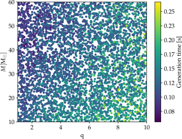
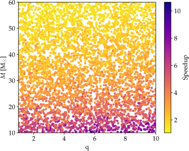
Figure 6: TEOBResumS generation time for 5000 time-domain waveforms without final interpolation on a uniform grid. The configurations are randomly sampled in $1<q<10$, $10<M[M_{\odot}]<60$ and $-1<\chi_{i}<1$ with starting GW frequency $f_{0}=10~{}{\rm Hz}$. Top panel: Computation time using the PA approximation to compute the dynamics. Bottom panel: Speed-up with respect to the same systems solving the complete ODEs.

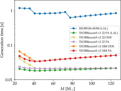
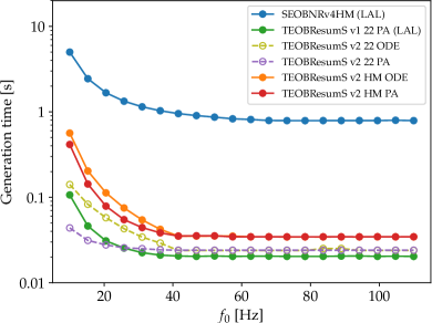
Figure 7: TEOBResumS generation time of time-domain waveforms interpolated on a uniform-in-time grid with rate equal to 4096 Hz. We show the most recent iteration, TEOBResumS v2, using either only the $\ell=m=2$ mode (22) or all the modes up to $\ell=8$ (HM). This is also run both employing the PA approximation (PA) or solving the full ODEs (ODE). We also show, as a comparison, the results for the LAL implementations of SEOBNRv4HM and TEOBResumS. The latter, TEOBResumS v1, uses the PA and does not include higher modes. The shown configurations correspond to $(q,\chi_{1},\chi_{2})=(2,+0.50,-0.30)$. Top panel: 20 waveforms with starting frequency $f_{0}=30~{}{\rm Hz}$ and total mass $25M_{\odot}\leq M\leq 125{\rm M}_{\odot}$. Bottom panel: 20 waveforms with $M=30~{}{\rm M_{\odot}}$ and varying $f_{0}$ between 10 and 110 Hz.

In this Section we show the performance of TEOBResumS using the PA approximation Nagar and Rettegno (2019). The latter is used to avoid part of the computation of Hamilton’s equations, that in the case of a nonprecessing system consist of 4 ordinary differential equations (ODEs). Its use can be extended to any EOB-based model, as shown in Sec. VI of Ref. Rettegno et al. (2019). Within TEOBResumS, the 8th PA order is generally used to compute the radial and angular momenta on a radial grid, starting at the initial radius $r_{0}$, ending at dimensionless separation $r=14$, with step $dr=0.1$. The other two dynamical variables, time and phase, are then calculated through an integration on the radial grid, essentially halving the number of necessary integrations. Beyond $r=14$ the approximation could become unreliable for certain configurations and hence the full ODEs are solved in the usual way The computational gain of using the PA approximation to compute full waveforms is preliminarily discussed in Appendices of Refs. Nagar et al. (2019b); Akcay et al. (2019), we present here a more detailed set of results.

In Fig. 6, we show the TEOBResumS waveform generation time and the speedup with respect to configurations when the 4 ODEs are solved for the whole evolution. As expected, the use of the PA approximation has a greater impact on longer waveforms (lower total mass). We can also note that, even without this speedup, TEOBResumS is already fast in the context of EOB-based models.

To put these times into perspective, in Fig. 7 we compare TEOBResumS to its equivalent higher modes model of the SEOBNR family, SEOBNRv4HM Bohé et al. (2017); Cotesta et al. (2018). This latter is implemented within the LIGO Algorithm Library (LAL) LIGO Scientific Collaboration (2018a, b) and, the time of writing, does not employ the PA approximation. The C implementation of TEOBResumS, denoted v2, is run with different settings: using all the modes up to $\ell=8$ or just the dominant $\ell=m=2$ one; employing the PA approximation for the dynamics or solving the full ODEs. These are compared to the LAL version of SEOBNRv4HM and of the same TEOBResumS. This older iteration, the TEOBResumS v1, already employed the PA approximation, but did not include higher modes nor NQC corrections in the flux. As we can expect, models which only include the $\ell=m=2$ multipole are found to be faster. At the same time, we can see that the PA approximation (that is never employed in TEOBResumS when systems would start at $r_{0}<14$) improves the performance for long waveforms. When compared to SEOBNRv4HM, we find that TEOBResumS is generally an order of magnitude faster.

We highlight that, in order to improve the SEOBNRv4HM performances, a reduced order model in the frequency domain has been developed Cotesta et al. (2020), that accelerates the waveform generation time by a factor of 100-200. In a similar effort, Ref. Schmidt et al. (2021) has recently applied machine learning methods to both TEOBResumS and SEOBNRv4 Bohé et al. (2017) and built time-domain models that achieve a speedup of 10 to 50 for TEOBResumS and about an order of magnitude more for SEOBNRv4, see Fig. 7 of Ref. Schmidt et al. (2021). This fact is consistent with our analysis of Fig. 7: it reflects the difference in computational cost of the two baseline models.

In conclusion, our timing analysis indicates that the native implementation of TEOBResumS using the PA approximation (including the v1 implementation distributed with LAL LIGO Scientific Collaboration (2018a)) is efficient enough to be used for parameter estimation, as we shall demonstrate in the following section.

V GW150914 analysis

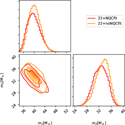
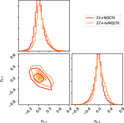
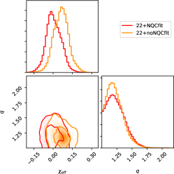
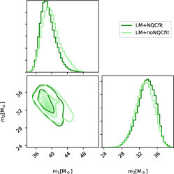
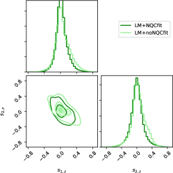
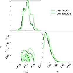
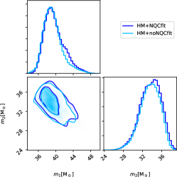
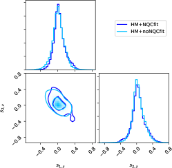
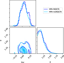
Figure 8: Parameter estimation of GW150914. Comparing parameter inference with and without NQC fits. It is interesting to note that the effect of the NQC is highly subdominant when all the higher modes up to $\ell=8$ are included in the waveform.

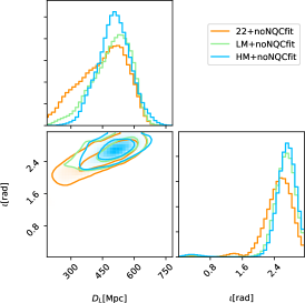
Figure 9: Parameter estimation of GW150914 without the NQC fits in radiation reaction. The figure compares posteriors of: (i) $\ell=m=2$ only waveform; (ii) multipolar waveform with all $\ell=m$ modes summed up to $\ell=5$; (iii) complete waveform with all modes up to $\ell=8$.

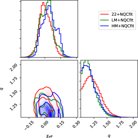
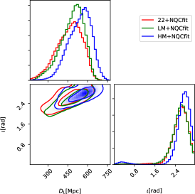
Figure 10: Parameter estimation of GW150914 with the NQC fits in radiation reaction. The figure compares posteriors of: (i) $\ell=m=2$ only waveform; (ii) multipolar waveform with all $\ell=m$ modes summed up to $\ell=5$; (iii) complete waveform with all modes up to $\ell=8$.

We ran a PE study on GW150914 using bajes Breschi et al. (2021). We employed the dynesty sampler with 1024 live points and tolerance of 0.1. We extracted the data from the GWOSC archive Abbott et al. (2019) and analyzed $16$ seconds of data around GPS time $1126259462$, with a sampling rate of 4096 Hz in the range of frequencies $[20,1024]$ Hz. We set the same prior distributions for all runs. The chirp mass prior was uniform in $[24,37]M_{\odot}$ and the mass ratio $q$ in $[1,8]$. We only considered aligned spins with an isotropic prior in the range $[-0.99,+0.99]$. We used a volumetric prior for the luminosity distance in $[100,800]$ Mpc.

Separate runs are performed with TEOBResumS, either including the new NQC fits in the radiation reaction or not. For each of the two cases, parameter estimation runs are performed with the $(2,2)$ mode only (22), the $\ell=m$ and $\ell\leq 5$ modes (LM), and with all the modes up to $\ell=m=8$ multipoles (HM). In this case, all the other subdominant modes except $(2,1)$, $(3,2)$, $(4,3)$ and $(4,2)$ do not use NR information to be completed through merger and ringdown, but only rely on the analytical EOB waveform (see e.g. Fig. 10 of Ref. Nagar et al. (2019a)). We used the PA approximation of the dynamics for all runs, as it is the default option for our implementation (e.g. Gamba et al. (2020a, b); Breschi et al. (2021).) Each one of these analyses took about 2 days on 8 CPUs. More details on the TEOBResumScomputational cost can be found in Appendix IV.

The results of such runs are listed in Table 1. The difference of using the NQC fits is highlighted in Fig. 8. Neglecting the NQC fits in the radiation reaction, that has a large impact on the EOB-NR unfaithfulness, has a very small effect on parameter estimation, despite the high SNR of GW150914. The only appreciable difference can be seen in the $\chi_{\rm eff}$ variable for the 22 run, which is more skewed towards 0 when NQC fits are used. It is interesting to note that the difference between using the NQC fits and not employing them tends to disappear when using more multipoles. Some effect in this direction was to be expected, since the NQC fits only affect the $\ell=m=2$ mode, which has a somewhat diminished importance when other multipoles are used.

Using the same data, we can attempt to determine whether this analysis is sensitive to the higher modes, given that the system is almost equal-mass and nonspinning. There are no appreciable differences in the system parameters when using higher order multipoles, apart from a small preference for a mass ratio closer to 1. Instead, using modes beyond the dominant $\ell=m=2$ one, helps to better constrain the source distance and inclination. In particular, the runs which employed a larger number of modes, seem to prefer larger distances and more face-on/away configuration. These results are compatible with what found in Ref. Kumar et al. (2019) using the NR surrogates NRSur7dq2 and NRSur7dq2HM. This difference in posteriors is shown in Figs. 9 and 10.

We conclude highlighting that using Bayes’ factors, we cannot determine a preference for any of the models used for these analyses (see again Table 1).

VI Conclusion

This work completes the description of the techniques employed in the current TEOBResumS waveform (v2) Nagar et al. (2018, 2020) and outlines a viable path towards the use of faithful EOB models in GW parameter estimation. Here, we highlighted the importance of: (i) including NQC corrections in the radiation reaction and (ii) using the post-adiabatic approximation to improve the computational efficiency of the inspiral.

The NQC fits developed here ensure an improved consistency between the EOB dynamics (radiation reaction flux) and the waveform without the need of an iterative procedure to determine the NQC parameters $(a^{(2,2)}_{1},a^{(2,2)}_{2})$. The EOB/NR unfaithfulness achieved with this NQC setting and with the use of the post-adiabatic approximation to the EOB dynamics is always below $0.01$, with 78.5% of the 611 NR waveforms below 0.001 (see right panel of Fig. 5).

The PA approximation, together with an efficient implementation, makes each version of TEOBResumS (including v1 distributed with LAL LIGO Scientific Collaboration (2018a)) suitable for parameter estimation in its native form, without the need of constructing surrogate or machine learning representations. The latter can provide significant further speed up Schmidt et al. (2021), but their construction becomes increasingly more complex as more physics effects are included (spin precession, eccentricity, etc).

The application of TEOBResumS to GW150914, that still represents one of the highest signal-to-noise ratio event observed thus far, indicates that the present techniques are well suited for the unbiased analysis of comparable-masses and moderately spinning binary black holes signals. In particular, the analysis is not sensitive to the inclusion of NQC fits in the radiation reaction, despite the inconsistency and far worse EOB/NR unfaithfulness of the model when these fits are not included. The inclusion of higher modes beyond the $\ell=m=2$ one has an appreciable effect only in giving a more stringent constraint of the source distance and inclination, as also seen with NR surrogates Kumar et al. (2019).

Future work should address the waveform systematics effects and limitation of current EOB models for larger mass-ratio and/or waveforms with larger spins. An important aspect in this respect, is to explore phasing, faithfulness and full parameter estimation altogether, as done for tidal effects in Gamba et al. (2020a), in order to identify which elements of the model require improvements and the connection between the phasing and the parameter estimation.

The current techniques can be immediately applied to include precessional effects Akcay et al. (2021) and tides Bernuzzi et al. (2015); Akcay et al. (2019); fast post-adiabatic multipolar waveforms with these features can be already generated with TEOBResumS. The same computationally efficient infrastructure of TEOBResumS is also shared by TEOBResumSGeneral Chiaramello and Nagar (2020); Nagar et al. (2021b, a), that deals with either eccentric inspirals (although without the PA approximation) or hyperbolic scatterings. Future work will also focus on rapid, and yet accurate, methods for the solution of the eccentric EOB dynamics Chiaramello and Nagar (2020); Nagar et al. (2021b, a), and on the extension of EOB to directly compute frequency-domain inspiral-merger-ringdown waveforms Gamba et al. (2020b).

Appendix A NR faithfulnesses with NQC iterations

This appendix reports for completeness the faithfulness published in Ref. Nagar et al. (2020) (Paper I) and obtained with the iterative NQC procedure and the full ODE integration. The plots are shown in Fig. 11 and can be directly compared to those shown in Fig. 4 in the main text, that are instead obtained with the fits for the NQC parameters $(a_{1}^{22},a_{2}^{22})$ entering the radiation reaction and the PA approximation to the numerical solution of the EOB Hamilton’s equations during the inspiral. The unfaithfulness plots are obtained using the most recent realization of the zero-detuned, high-power noise spectral density of Advanced LIGO aLI .

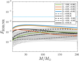
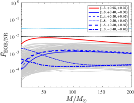
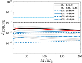
Figure 11: EOB/NR unfaithfulness for the $\ell=m=2$ mode using all currently available SXS NR simulations (left and middle panel) and a selection of BAM simulations (right panel). as published in Ref. Nagar et al. (2020) (Paper I). The NQC parameters are determined iteratively and included in the radiation reaction. The Hamilton equation of motion are solved numerically without using the post-adibatic approximation. Left panel: computation using SXS waveforms publicly released before February 3, 2019. Middle panel: using SXS waveform data publicly released after February 3, 2019. $\bar{F}^{\rm max}_{\rm EOB/NR}$ is always below $0.4\%$ except for a single outlier, red online, that however never exceeds $0.85\%$. The plot includes five exceptionally long waveforms, each one developing more than 139 GW cycles before merger, SXS:BBH:1412, 1413, 1414, 1415 and 1416 (blue online). Right panel: same computation done with a few BAM waveform data that include configurations with mass ratio $q=18$. See Ref. Nagar et al. (2020) for further details.

Appendix B NQC fits of $(a^{(2,2)}_{1},a^{(2,2)}_{2})$

This appendix summarizes the NQC fits performed in this work. The fits are performed hierarchically in different sectors of the parameter. All fits have been performed with fitnlm of Matlab. The superscript $(2,2)$ is dropped in the notation in this appendix.

B.1 Non-spinning sector

The fits in the non-spinning sector are obtained with a total of $27$ waveforms, for mass-ratios $1\leq q\leq 30$. The coefficient $a_{1}$ is fitted against $X_{12}^{2}=\left(1-4\nu\right)^{2}$ with the template

$$a_{1}\;\;\;\; =\frac{a_{1}^{q=1}}{1+b^{a_{1}}_{1}X_{12}^{2}+b^{a_{1}}_{2}X_{12}^{4}}$$ (6)

with

$$a_{1}^{q=1} =\;\;\,0.070974$$

$$b^{a_{1}}_{1}\,\;\; =\;\;\,0.786350$$

$$b^{a_{1}}_{2}\,\;\; =-9.085105\ .$$

The value of $a_{1}^{q=1}$ is extracted from $q=1$ NR data.

The coefficient $a_{2}$ in the non-spinning sector is fitted against $X_{12}=\sqrt{1-4\nu}$ with the template

$$a_{2}\;\;\;\; =a_{2}^{q=1}\frac{1+b^{a_{2}}_{1}X_{12}+b^{a_{2}}_{2}X_{12}^{2}}{1+b^{a_{2}}_{3}X_{12}}$$ (7)

with

$$a_{2}^{q=1} =\;\;\,1.315133$$

$$b^{a_{2}}_{1}\,\;\; =-0.324849$$

$$b^{a_{2}}_{2}\,\;\; =-0.304506$$

$$b^{a_{2}}_{3}\,\;\; =-0.371614\ .$$

The value of $a_{2}^{q=1}$ is extracted from $q=1$ NR data.

B.2 Equal-mass sector

Equal-mass data are defined by $\nu>0.2485$. A total of $40$ waveforms with spins $-0.98\leq\chi_{1,2}\leq 0.99$ are used to obtain the fits of the equal-mass region. The coefficient $a_{1}$ in the equal-mass cases is fitted with the template:

$$a_{1}=c^{a_{1}}_{0}\frac{1+c^{a_{1}}_{1}\hat{S}+c^{a_{1}}_{2}\hat{S}^{2}+c^{a_{1}}_{3}\hat{S}^{3}+c^{a_{1}}_{4}\hat{S}^{4}}{1+c^{a_{1}}_{5}\hat{S}+c^{a_{1}}_{6}\hat{S}^{2}+c^{a_{1}}_{7}\hat{S}^{3}}\ .$$ (8)

with the coefficients:

$$c^{a_{1}}_{0} =\,\;0.121187 \;\;\;c^{a_{1}}_{1} =\,\;-5.950663$$

$$c^{a_{1}}_{2} =\,\;9.420324 \;\;\;c^{a_{1}}_{3} =-10.601339$$

$$c^{a_{1}}_{4} =17.641549 \;\;\;c^{a_{1}}_{5} =\,\;-5.684777$$

$$c^{a_{1}}_{6} =10.910451 \;\;\;c^{a_{1}}_{7} =\,\;-6.867377\ .$$

The coefficient $a_{2}$ is fitted to the same template. The fitted coefficients are:

$$c^{a_{2}}_{0} =\;\;\,1.331703 \;\;\;c^{a_{2}}_{1} =-4.237724$$

$$c^{a_{2}}_{2} =\;\;\,1.786023 \;\;\;c^{a_{2}}_{3} =\,\,10.546205$$

$$c^{a_{2}}_{4} =-9.698233 \;\;\;c^{a_{2}}_{5} =-6.225823$$

$$c^{a_{2}}_{6} =\,\,13.209381 \;\;\;c^{a_{2}}_{7} =-9.402513\ .$$

B.3 Sector with mass ratio $1<q<4$

In this sector the fit of $a_{1}$ differs in two ways from the previous: (i) the fit is factorized in a spinning part $a_{1}^{S}$ and a non-spinning part $a_{1}^{0}$, and (ii) the fit uses the spin variable $\hat{S}_{\nu}\equiv\hat{S}/(1-2\nu)$. The full template is:

$$a_{1} =a_{1}^{0}\cdot a_{1}^{S}\ ,$$ (9)

$$a^{0}_{1} =d^{a_{1}}_{0}\frac{1+d^{a_{1}}_{1}\nu+d^{a_{1}}_{2}\nu^{3}}{1+d^{a_{1}}_{3}\nu}\ ,$$ (10)

$$a^{S}_{1} =\frac{1+d^{a_{1}}_{4}\hat{S}_{n}+d^{a_{1}}_{5}\hat{S}_{\nu}^{2}+d^{a_{1}}_{6}\hat{S}_{\nu}^{3}+d^{a_{1}}_{7}\hat{S}_{\nu}^{4}}{1+d^{a_{1}}_{8}\hat{S}_{\nu}+d^{a_{1}}_{9}\hat{S}_{\nu}^{2}+d^{a_{1}}_{10}\hat{S}_{\nu}^{3}}\ .$$ (11)

The fitted coefficients take the values of $a_{1}^{0}$ are:

$$d^{a_{1}}_{0} =\,\;0.26132647 \;\;\;d^{a_{1}}_{1} =-4.90302367$$

$$d^{a_{1}}_{2} =20.67036124 \;\;\;d^{a_{1}}_{3} =-3.17109808\ .$$

Note these coefficients are fitted to waveforms for which $\chi_{2}=\pm 0.01$ and $\chi_{1}$ is chosen such that $\hat{S}_{\nu}=0$. This approach is taken also for all of the following non-spinning factor fits. In total 70 waveforms with $\hat{S}_{n}=0$ and further $454$ with spin $-0.9<\chi_{1,2}\leq 0.99$. Of these $160$ are focused on the high positive region, $0.8\leq\chi_{1,2}\leq 0.99$.

The fitted coefficients of $a_{1}^{S}$ are:

$$d^{a_{1}}_{4} =-3.082861 \;\;\;d^{a_{1}}_{5} =2.169948$$

$$d^{a_{1}}_{6} =-0.636353 \;\;\;d^{a_{1}}_{7} =0.741419$$

$$d^{a_{1}}_{8} =-2.843896 \;\;\;d^{a_{1}}_{9} =2.709697$$

$$d^{a_{1}}_{10} =-0.832894 \ .$$

The coefficient $a_{2}$ is fitted in a factorized form as well. Additionally, it holds an explicit dependency of $a_{2}^{S}$ on $\nu$:

$$a_{2} =a_{2}^{0}\cdot a_{2}^{S}\ ,$$ (12)

$$a^{0}_{2} =d^{a_{2}}_{0}\frac{1+d^{a_{2}}_{1}\nu+d^{a_{2}}_{2}\nu^{3}}{1+d^{a_{2}}_{3}\nu}\ ,$$ (13)

$$a^{S}_{2} =\frac{1+d^{a_{2}}_{4}\hat{S}_{\nu}+d^{a_{2}}_{5}\hat{S}_{\nu}^{2}+d^{a_{2}}_{6}\hat{S}_{\nu}^{3}+d^{a_{2}}_{7}\hat{S}_{\nu}^{4}}{1+d^{a_{2}}_{8}\hat{S}_{\nu}+d^{a_{2}}_{9}\hat{S}_{\nu}^{2}+d^{a_{2}}_{10}\hat{S}_{\nu}^{3}}\ ,$$ (14)

$$d^{a_{2}}_{i} =d^{a_{2}}_{i,0}\left(1+d^{a_{2}}_{i,1}\nu\right),\ for\ i=4,...,10\ .$$ (15)

The fitted coefficients of $a_{2}^{0}$ are:

$$d^{a_{2}}_{0} =\;\;\,1.03364144 \;\;\;d^{a_{2}}_{1} =-3.46191440$$

$$d^{a_{2}}_{2} =-7.86652243 \;\;\;d^{a_{2}}_{3} =-3.96268815\ .$$

The fitted coefficients of $a_{2}^{S}$ are:

$$d^{a_{2}}_{4,0} =\;\;\,0.036452 \;\;\;d^{a_{2}}_{4,1} =-64.360789$$

$$d^{a_{2}}_{5,0} =\;\;\,0.275707 \;\;\;d^{a_{2}}_{5,1} =-34.573145$$

$$d^{a_{2}}_{6,0} =-0.113951 \;\;\;d^{a_{2}}_{6,1} =\;\;\,\,\;0$$

$$d^{a_{2}}_{7,0} =-2.531304 \;\;\;d^{a_{2}}_{7,1} =\,\;-7.691661$$

$$d^{a_{2}}_{8,0} =-1.025824 \;\;\;d^{a_{2}}_{8,1} =\;\;\,\,\;4.237539$$

$$d^{a_{2}}_{9,0} =\;\;\,0.593579 \;\;\;d^{a_{2}}_{9,1} =\;\;\,\,\;1.661809$$

$$d^{a_{2}}_{10,0} =-0.939736 \;\;\;d^{a_{2}}_{10,1} =\,\;-6.333442\ .$$

$d^{a_{2}}_{6,1}$ is set to $0$ prior to the evaluation of the fit to improve the convergence of the fit.

B.4 Sector with mass ratio $q\geq 4$

For the following fits a similar approach to was taken as above. A total of $44$ with $\hat{S}_{n}=0$ have been generated. $186$ waveforms with $-0.99\leq\chi_{1,2}\leq 0.99$ have been used to capture the $q=4$ behavior accurately. $1470$ further waveforms with $-0.99\leq\chi_{1,2}\leq 0.85$ have been used to fit the extrapolation of the $q=4$ fit up to mass ratio $q=30$. The coefficient $a_{1}$ for $q\geq 4$ has an additional feature. The explicit $\nu$ dependence is fitted through $x_{\nu}=\nu-0.16$. The full template is:

$$a_{1} =a_{1}^{0}\cdot a_{1}^{S}\ ,$$ (16)

$$a^{0}_{1} =e^{a_{1}}_{0}\frac{1+e^{a_{1}}_{1}\nu+e^{a_{1}}_{2}\nu^{3}}{1+e^{a_{1}}_{3}\nu}\ ,$$ (17)

$$a^{S}_{1} =\frac{1+e^{a_{1}}_{4}\hat{S}_{\nu}+e^{a_{1}}_{5}\hat{S}_{\nu}^{2}+e^{a_{1}}_{6}\hat{S}_{\nu}^{3}+e^{a_{1}}_{7}\hat{S}_{\nu}^{4}}{1+e^{a_{1}}_{8}\hat{S}_{\nu}+e^{a_{1}}_{9}\hat{S}_{\nu}^{2}+e^{a_{1}}_{10}\hat{S}_{\nu}^{3}}\ ,$$ (18)

$$e^{a_{1}}_{i} =e^{a_{1}}_{i,0}\frac{1+e^{a_{1}}_{i,1}x_{\nu}}{1+e^{a_{1}}_{i,2}x_{\nu}},\ for\ i=4,...,10\ .$$ (19)

The fitted $a_{1}^{0}$ coefficients are:

$$e^{a_{1}}_{0} =\;\;\,0.341803 \;\;\;e^{a_{1}}_{1} =-1.350488$$

$$e^{a_{1}}_{2} =-6.353357 \;\;\;e^{a_{1}}_{3} =\;\;\,2.216156\ .$$

The coefficients of $a_{1}^{S}$ are fitted in 2 steps. First, for $q=4$ and second, an extrapolated fit from there. The coefficients $e^{a_{1}}_{i,0}$ are fitted to $q=4$:

$$e^{a_{1}}_{4,0} =-2.287721 \;\;\;e^{a_{1}}_{5,0} =-0.598451$$

$$e^{a_{1}}_{6,0} =\;\;\,0.766069 \;\;\;e^{a_{1}}_{7,0} =\;\;\,1.857169$$

$$e^{a_{1}}_{8,0} =-2.035234 \;\;\;e^{a_{1}}_{9,0} =\;\;\,0.836427$$

$$e^{a_{1}}_{10,0} =\;\;\,0.297476 \ .$$

The remaining coefficients model the extrapolation of the spin dependence to larger mass ratios and are:

$$e^{a_{1}}_{4,1} =\;\;\,\;\,7.650946 \;\;\;e^{a_{1}}_{4,2} =\;\;\,\;\,7.106992$$

$$e^{a_{1}}_{5,1} =-60.630748 \;\;\;e^{a_{1}}_{5,2} =-69.630357$$

$$e^{a_{1}}_{6,1} =\;\;\,47.114247 \;\;\;e^{a_{1}}_{6,2} =\;\;\,\;\,5.733002$$

$$e^{a_{1}}_{7,1} =-12.905707 \;\;\;e^{a_{1}}_{7,2} =\;\;\,\;\,5.045688$$

$$e^{a_{1}}_{8,1} =\;\;\,\;\,3.515869 \;\;\;e^{a_{1}}_{8,2} =\;\;\,\;\,1.564146$$

$$e^{a_{1}}_{9,1} =\;\;\,\;\,0.642864 \;\;\;e^{a_{1}}_{9,2} =\;\;\,\;\,2.947890$$

$$e^{a_{1}}_{10,1} =\;\;\,31.023038 \;\;\;e^{a_{1}}_{10,2} =\;\;\,\;\,1.829543\ .$$

The coefficient $a_{2}$ is fitted similarly with the template:

$$a_{2} =a_{2}^{0}\cdot a_{2}^{S}\ ,$$ (20)

$$a^{0}_{2} =e^{a_{2}}_{0}\frac{1+e^{a_{2}}_{1}\nu+e^{a_{2}}_{2}\nu^{3}}{1+e^{a_{2}}_{3}\nu}\ ,$$ (21)

$$a^{S}_{2} =\frac{1+e^{a_{2}}_{4}\hat{S}_{\nu}+e^{a_{2}}_{5}\hat{S}_{\nu}^{2}+e^{a_{2}}_{6}\hat{S}_{\nu}^{3}+e^{a_{2}}_{7}\hat{S}_{\nu}^{4}}{1+e^{a_{2}}_{8}\hat{S}_{\nu}+e^{a_{2}}_{9}\hat{S}_{\nu}^{2}}\ ,$$ (22)

$$e^{a_{2}}_{i} =e^{a_{2}}_{i,0}\frac{1+e^{a_{2}}_{i,1}x_{\nu}}{1+e^{a_{2}}_{i,2}x_{\nu}},\ for\ i=4,...,9\ .$$ (23)

The fitted $a_{2}^{0}$ coefficients are:

$$e^{a_{2}}_{0} =\;\,\;\;\,0.929192 \;\;\;e^{a_{2}}_{1} =\;\;\,1.334263$$

$$e^{a_{2}}_{2} =-26.389790 \;\;\;e^{a_{2}}_{3} =-1.289984\ .$$

The coefficients of $a_{2}^{S}$ are fitted in 2 steps as well. The coefficients $e^{a_{2}}_{i,0}$ have been fitted to $q=4$:

$$e^{a_{2}}_{4,0} =-0.886561 \;\;\;e^{a_{2}}_{5,0} =-1.953955$$

$$e^{a_{2}}_{6,0} =\;\;\,1.366537 \;\;\;e^{a_{2}}_{7,0} =\;\;\,0.950212$$

$$e^{a_{2}}_{8,0} =-2.531000 \;\;\;e^{a_{2}}_{9,0} =\;\;\,1.723991\ .$$

The remaining coefficients model the extrapolation of the spin dependence to larger mass ratios and are:

$$e^{a_{2}}_{4,1} =\;\;\,15.871482 \;\;\;e^{a_{2}}_{4,2} =\;\,\;\;\,5.066190$$

$$e^{a_{2}}_{5,1} =\;\,\;\;\,7.168498 \;\;\;e^{a_{2}}_{5,2} =\;\,\;\;\,6.709490$$

$$e^{a_{2}}_{6,1} =\;\;\,18.583382 \;\;\;e^{a_{2}}_{6,2} =\;\,\;\;\,5.764512$$

$$e^{a_{2}}_{7,1} =-14.038564 \;\;\;e^{a_{2}}_{7,2} =-17.126231$$

$$e^{a_{2}}_{8,1} =\;\,\;\;\,6.387917 \;\;\;e^{a_{2}}_{8,2} =\;\,\;\;\,3.438456$$

$$e^{a_{2}}_{9,1} =\;\,\;\;\,8.867098 \;\;\;e^{a_{2}}_{9,2} =\;\,\;\;\,2.910938\ .$$

References

- Acernese et al. (2015) F. Acernese et al. (VIRGO), Class. Quant. Grav. 32, 024001 (2015), arXiv:1408.3978 [gr-qc] .
- Aasi et al. (2015) J. Aasi et al. (LIGO Scientific), Class. Quant. Grav. 32, 074001 (2015), arXiv:1411.4547 [gr-qc] .
- Abbott et al. (2020) R. Abbott et al. (LIGO Scientific, Virgo), (2020), arXiv:2010.14527 [gr-qc] .
- Buonanno and Damour (1999) A. Buonanno and T. Damour, Phys. Rev. D59, 084006 (1999), arXiv:gr-qc/9811091 .
- Buonanno and Damour (2000) A. Buonanno and T. Damour, Phys. Rev. D62, 064015 (2000), arXiv:gr-qc/0001013 .
- Damour et al. (2000) T. Damour, P. Jaranowski, and G. Schaefer, Phys. Rev. D62, 084011 (2000), arXiv:gr-qc/0005034 [gr-qc] .
- Damour (2001) T. Damour, Phys. Rev. D64, 124013 (2001), arXiv:gr-qc/0103018 .
- Damour et al. (2015) T. Damour, P. Jaranowski, and G. Schäfer, Phys. Rev. D91, 084024 (2015), arXiv:1502.07245 [gr-qc] .
- Nagar and Rettegno (2019) A. Nagar and P. Rettegno, Phys. Rev. D99, 021501 (2019), arXiv:1805.03891 [gr-qc] .
- Nagar et al. (2018) A. Nagar et al., Phys. Rev. D98, 104052 (2018), arXiv:1806.01772 [gr-qc] .
- Cotesta et al. (2018) R. Cotesta, A. Buonanno, A. Bohé, A. Taracchini, I. Hinder, and S. Ossokine, Phys. Rev. D98, 084028 (2018), arXiv:1803.10701 [gr-qc] .
- Nagar et al. (2019a) A. Nagar, G. Pratten, G. Riemenschneider, and R. Gamba, (2019a), arXiv:1904.09550 [gr-qc] .
- Nagar et al. (2020) A. Nagar, G. Riemenschneider, G. Pratten, P. Rettegno, and F. Messina, (2020), arXiv:2001.09082 [gr-qc] .
- Ossokine et al. (2020) S. Ossokine et al., (2020), arXiv:2004.09442 [gr-qc] .
- Schmidt et al. (2021) S. Schmidt, M. Breschi, R. Gamba, G. Pagano, P. Rettegno, G. Riemenschneider, S. Bernuzzi, A. Nagar, and W. Del Pozzo, Phys. Rev. D 103, 043020 (2021), arXiv:2011.01958 [gr-qc] .
- Nagar et al. (2021a) A. Nagar, A. Bonino, and P. Rettegno, (2021a), arXiv:2101.08624 [gr-qc] .
- Nagar et al. (2021b) A. Nagar, P. Rettegno, R. Gamba, and S. Bernuzzi, Phys. Rev. D 103, 064013 (2021b), arXiv:2009.12857 [gr-qc] .
- Gamba et al. (2020a) R. Gamba, M. Breschi, S. Bernuzzi, M. Agathos, and A. Nagar, preprint (ArXiv:2009.08467) , arXiv:2009.08467 (2020a), arXiv:2009.08467 [gr-qc] .
- Damour et al. (2002) T. Damour, E. Gourgoulhon, and P. Grandclement, Phys. Rev. D 66, 024007 (2002), arXiv:gr-qc/0204011 .
- Damour and Nagar (2007) T. Damour and A. Nagar, Phys. Rev. D76, 064028 (2007), arXiv:0705.2519 [gr-qc] .
- Damour et al. (2008a) T. Damour, A. Nagar, E. N. Dorband, D. Pollney, and L. Rezzolla, Phys. Rev. D77, 084017 (2008a), arXiv:0712.3003 [gr-qc] .
- Damour et al. (2008b) T. Damour, A. Nagar, M. Hannam, S. Husa, and B. Brügmann, Phys. Rev. D78, 044039 (2008b), arXiv:0803.3162 [gr-qc] .
- Damour and Nagar (2009) T. Damour and A. Nagar, Phys. Rev. D79, 081503 (2009), arXiv:0902.0136 [gr-qc] .
- Damour et al. (2009) T. Damour, B. R. Iyer, and A. Nagar, Phys. Rev. D79, 064004 (2009), arXiv:0811.2069 [gr-qc] .
- Messina et al. (2018) F. Messina, A. Maldarella, and A. Nagar, Phys. Rev. D97, 084016 (2018), arXiv:1801.02366 [gr-qc] .
- Bohé et al. (2017) A. Bohé et al., Phys. Rev. D95, 044028 (2017), arXiv:1611.03703 [gr-qc] .
- Rettegno et al. (2019) P. Rettegno, F. Martinetti, A. Nagar, D. Bini, G. Riemenschneider, and T. Damour, (2019), arXiv:1911.10818 [gr-qc] .
- Damour et al. (2013) T. Damour, A. Nagar, and S. Bernuzzi, Phys.Rev. D87, 084035 (2013), arXiv:1212.4357 [gr-qc] .
- Breschi et al. (2021) M. Breschi, R. Gamba, and S. Bernuzzi, preprint (ArXiv:2102.00017) (2021), arXiv:2102.00017 [gr-qc] .
- Nagar et al. (2019b) A. Nagar, F. Messina, P. Rettegno, D. Bini, T. Damour, A. Geralico, S. Akcay, and S. Bernuzzi, Phys. Rev. D99, 044007 (2019b), arXiv:1812.07923 [gr-qc] .
- Gamba et al. (2020b) R. Gamba, S. Bernuzzi, and A. Nagar, preprint (ArXiv:2012.00027) , arXiv:2012.00027 (2020b), arXiv:2012.00027 [gr-qc] .
- Lackey et al. (2017) B. D. Lackey, S. Bernuzzi, C. R. Galley, J. Meidam, and C. Van Den Broeck, Phys. Rev. D95, 104036 (2017), arXiv:1610.04742 [gr-qc] .
- Cotesta et al. (2020) R. Cotesta, S. Marsat, and M. Pürrer, Phys. Rev. D 101, 124040 (2020), arXiv:2003.12079 [gr-qc] .
- LIGO Scientific Collaboration (2018a) LIGO Scientific Collaboration, “LIGO Algorithm Library - LALSuite,” free software (GPL) (2018a).
- Nagar et al. (2017) A. Nagar, G. Riemenschneider, and G. Pratten, Phys. Rev. D96, 084045 (2017), arXiv:1703.06814 [gr-qc] .
- Albertini and Nagar (2021) A. Albertini and A. Nagar, (2021), arXiv:In preparation [gr-qc] .
- Boyle et al. (2008) M. Boyle, A. Buonanno, L. E. Kidder, A. H. Mroue, Y. Pan, et al., Phys.Rev. D78, 104020 (2008), arXiv:0804.4184 [gr-qc] .
- Bernuzzi et al. (2011a) S. Bernuzzi, A. Nagar, and A. Zenginoglu, Phys.Rev. D83, 064010 (2011a), arXiv:1012.2456 [gr-qc] .
- Bernuzzi et al. (2011b) S. Bernuzzi, A. Nagar, and A. Zenginoglu, Phys.Rev. D84, 084026 (2011b), arXiv:1107.5402 [gr-qc] .
- Harms et al. (2014) E. Harms, S. Bernuzzi, A. Nagar, and A. Zenginoglu, Class.Quant.Grav. 31, 245004 (2014), arXiv:1406.5983 [gr-qc] .
- Nagar et al. (2016) A. Nagar, T. Damour, C. Reisswig, and D. Pollney, Phys. Rev. D93, 044046 (2016), arXiv:1506.08457 [gr-qc] .
- Damour et al. (2012) T. Damour, A. Nagar, D. Pollney, and C. Reisswig, Phys.Rev.Lett. 108, 131101 (2012), arXiv:1110.2938 [gr-qc] .
- (43) “LIGO Document T0900288-v3,” https://dcc.ligo.org/cgi-bin/DocDB/ShowDocument?docid=2974, Advanced LIGO anticipated sensitivity curves.
- Akcay et al. (2019) S. Akcay, S. Bernuzzi, F. Messina, A. Nagar, N. Ortiz, and P. Rettegno, Phys. Rev. D99, 044051 (2019), arXiv:1812.02744 [gr-qc] .
- LIGO Scientific Collaboration (2018b) LIGO Scientific Collaboration, “LIGO Algorithm Library - LALSuite,” free software (GPL) (2018b).
- Abbott et al. (2019) R. Abbott et al. (LIGO Scientific, Virgo), (2019), arXiv:1912.11716 [gr-qc] .
- Kumar et al. (2019) P. Kumar, J. Blackman, S. E. Field, M. Scheel, C. R. Galley, M. Boyle, L. E. Kidder, H. P. Pfeiffer, B. Szilagyi, and S. A. Teukolsky, Phys. Rev. D 99, 124005 (2019), arXiv:1808.08004 [gr-qc] .
- Akcay et al. (2021) S. Akcay, R. Gamba, and S. Bernuzzi, Phys. Rev. D 103, 024014 (2021), arXiv:2005.05338 [gr-qc] .
- Bernuzzi et al. (2015) S. Bernuzzi, A. Nagar, T. Dietrich, and T. Damour, Phys.Rev.Lett. 114, 161103 (2015), arXiv:1412.4553 [gr-qc] .
- Chiaramello and Nagar (2020) D. Chiaramello and A. Nagar, Phys. Rev. D 101, 101501 (2020), arXiv:2001.11736 [gr-qc] .
- (51) “Updated Advanced LIGO sensitivity design curve,” https://dcc.ligo.org/LIGO-T1800044/public.