A Decomposition Model for Stereo Matching

Abstract

In this paper, we present a decomposition model for stereo matching to solve the problem of excessive growth in computational cost (time and memory cost) as the resolution increases. In order to reduce the huge cost of stereo matching at the original resolution, our model only runs dense matching at a very low resolution and uses sparse matching at different higher resolutions to recover the disparity of lost details scale-by-scale. After the decomposition of stereo matching, our model iteratively fuses the sparse and dense disparity maps from adjacent scales with an occlusion-aware mask. A refinement network is also applied to improving the fusion result. Compared with high-performance methods like PSMNet and GANet, our method achieves $10-100\times$ speed increase while obtaining comparable disparity estimation results.

1 Introduction

Stereo matching aims to estimate the disparity from a pair of images. It has various downstream applications, such as 3D reconstruction, AR, autonomous driving, robot navigation, etc. Despite years of research on stereo matching, many state-of-the-art methods still face the problem of excessive growth in computational cost and memory consumption as the resolution increases. This problem limits the ability of existing methods to process high-resolution images, and restricts the use of stereo matching methods in practical situations with memory/speed constraints.

Figure 1: As the resolution increases, the growth in time cost of state-of-the-art methods on one 1080 Ti GPU with 11GB of memory. The stopped growth of some curves is because the corresponding method cannot run at the expected resolution on the GPU. Compared to GANet [48], our model is 100 times faster. Compared to PSMNet [5], our model achieves almost $15\times$ speed increase. Compared to DeepPruner [8], our model achieves almost twice the running speed and lower memory consumption.

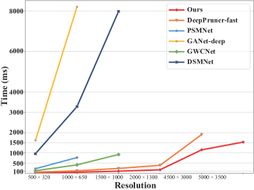
In this paper, we propose a decomposition model for stereo matching. Compared with the excessive growth of many state-of-the-art methods, our model reduces the growth rate by several orders of magnitude as shown in Figure 1. The design of our model is inspired by the following two observations:

(1) It is not necessary to estimate the disparity of all pixels at the highest resolution, such as the disparities on the wall and the floor. As long as the content is not significantly lost during downsampling, the disparity of most areas can be efficiently estimated at low resolution, and then refined at high resolution.

(2) It only needs to consider the disparity estimation of some image details that are lost during downsampling. Fortunately, those lost details are sparse, and their stereo matching is also sparse (i.e., the lost details in the left image mostly only match the lost details in the right image). The sparse matching means less time and memory cost compared to the dense matching.

Based on the first observation, our model only runs dense matching at a very low resolution (such as $20\times 36$, called reference resolution), ensuring disparity estimation for most regions that are not lost during downsampling. Based on the second observation, our model uses a series of sparse matching, each at a suitable higher resolution, to recover the disparity of lost details scale-by-scale. By decomposing the original stereo matching into a dense matching at the lowest resolution and a series of sparse matching at higher resolutions, the huge cost of original stereo matching can be significantly reduced.

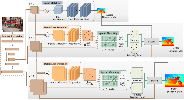
The specific pipeline of our model is shown in Figure 2. Our model uses a full cost volume and a cost regularization for dense matching at the reference resolution. From the reference resolution, a series of operations are performed scale-by-scale, until the original input resolution is reached. These operations include four modules: detail loss detection, sparse matching, disparity upsampling, and disparity fusion. The corresponding implementation of the four modules are as follows: (1) In the detail loss detection module, the lost image details are learned unsupervised based on the square difference between deep features from adjacent scales. (2) In the sparse matching module, the sparse disparity map is estimated via cross-correlation and soft-max under the guidance of detected lost details. (3) In the disparity upsampling module, the estimated disparity map from the previous scale is upsampled to the resolution at the current scale via content-aware weights. (4) In the disparity fusion module, the results of the disparity upsampling module and sparse matching module are fused via an occlusion-aware soft mask. A refinement network is also used in this module to improve the fused disparity map.

We analyze the complexity of stereo matching in this paper. For convenience, we define the complexity of matching as the size of the search space [21]. We prove that the complexity of original dense stereo matching grows cubically as the input resolution increases, while the complexity of sparse matching in our model only grows logarithmically. In our model, the complexity of dense matching at the reference resolution is fixed, and independent of the input resolution. At the same time, the three other operations, i.e., detail loss detection, disparity upsampling, and disparity fusion, could be efficiently implemented.

In the experiment, we compare our model with state-of-the-art methods over the growth in computation cost and memory consumption. The results show that our model reduces the growth rate by several orders of magnitude. We also compare our model with state-of-the-art methods on Scene Flow dataset [23], KITTI 2015 dataset [24, 25, 26], and Middlebury dataset [34]. The results show that our model is comparable to or even better than state-of-the-art methods with much faster running time and much lower memory cost.

2 Related Work

Stereo Matching has been studied for decades [39, 22, 33]. In the early stage, researchers focus on the analysis of binocular vision and the building of its computation framework [39, 30, 16, 22, 29]. Later, a series of traditional stereo matching approaches are proposed to improve the framework, including local model [2, 13, 45], global model [4, 19, 36] and semi-global model [15, 35]. Recently, deep-learning-based approaches have emerged and play the most important role in stereo matching [47, 23, 17, 5]. Although both traditional methods and deep learning methods have achieved great performance, they still suffer from the problem of excessive growth in computation cost as the resolution increases.

Traditional Methods. In order to solve the problem, researchers propose many approaches to reduce the size of search space, by either improving the operations in dense matching, or turning for the sparse-to-dense methods. In the first perspective, researchers propose to reduce the complexity of cost aggregation in terms of the size of image [27, 9], matching window [31], or disparity space [28, 9]. The semi-global matching (SGM) [14] is also proposed to approximate the global energy function with pathwise optimizations from all directions. Different from them improving the operations on dense matching, we replace the dense matching at high resolution with sparse matching to reduce the complexity. In the second perspective, researchers mainly focus on the sparse nature in stereo matching [10, 3, 12, 21, 35]. They propose to compute the sparse disparity map over the extracted key points, and then infer the dense disparity map based on the sparse result, like efficient large-scale stereo [10] and local plane sweeps [35]. PatchMatch-based methods [3, 12, 21] are similar to them but mostly generate the sparse result via random initialization. They are based on the assumption that at least one pixel of the areas is initialized with a label close to the ground truth. Different from them only using sparse matching with local information, we use dense matching at the lowest resolution to provide global information and use sparse matching to recover the local details at high resolution.

Deep Methods In deep learning methods, researchers try to solve the excessive growth in computation cost and memory consumption from two aspects, light-weight network, and improved the computaion with cost volume. In the first aspect, most researchers replace the expensive operations on cost volume with a specially designed module [48, 43, 40, 20]. Some others also improve the whole architecture of network to achieve less computation cost [18, 41, 37]. However, the above methods ignore the influence of cost volume. The cost volume will result in cubical growth of computation cost and memory consumption when resolution increasing. In order to further resolve the problem, researchers propose to improve the computaion with cost volume based on the assumption where most content of the cost volume is redundant. They mainly improve the computaion with cost volume via narrowing the disparity space based on the initial estimation and then upsample the result from coarse to fine [44, 8, 6, 46, 7, 11]. Among them, DeepPruner [8] achieves great performance. They use the minimum and maximum disparity regressed by CNN to sample fixed size candidate disparities for the matching at a higher resolution. They also design a light-weight architecture for more efficient cost aggregation and regression. However, they ignore the computation of details at high resolution which are lost in low-resolution matching and are difficult to be recovered with a small size of sampling. Different from the above coarse-to-fine methods, our model is coarse+fine. Instead of only depending on the initial estimation at coarse scale to generate the details at fine scale, we preserve the details in the decomposition of stereo matching. Thus, our model could perform the dense matching at a very low resolution to reduce the search space size but without significant information loss. Furthermore, we resolve the problem from a new view and propose a new pipeline for stereo matching where all the above methods could be integrated into each step in our model to build a more powerful stereo matching, which is a good supplement to the current research mainstream.

Figure 2: Overview of our model. Given a pair of images, we first extract the feature map for the matching at level $l$. We then run the dense matching at the lowest resolution $l=0$ and use sparse matching at different higher resolutions $l\geq 1$. For the computed dense and sparse disparity maps, we fuse them hierarchically to recover the dense disparity map at the original resolution $l=L$. The fusion is composed of disparity upsampling, disparity fusion, and refinement. ⓦ is the warping operation between left and right view. -⃝ represents the computation of the square difference between feature maps from adjacent levels. For details please refer to our method part.

3 Method

3.1 Multi-Scale Stereo Matching

Stereo matching is a dense correspondence problem. It is typically modeled as an exhaustive search process between different areas from left and right views with multi-scale analysis which is used to reduce the ambiguity caused by ill-posed areas. In order to better model this process, we recognize the image as a set of areas $\{A_{l}\}_{l=0}^{l=L}$ where $A_{l}$ represents all areas at each scale/level $l$. The exhausting search process is then modeled as

$$D_{L} =\mathcal{F}(\acute{A}_{L},\grave{A}_{L},D_{L-1}),$$ (1)

$$\ldots$$

$$D_{1} =\mathcal{F}(\acute{A}_{1},\grave{A}_{1},D_{0}),$$

$$D_{0} =\mathcal{F}(\acute{A}_{0},\grave{A}_{0}),$$

$$\tilde{D} =\phi(D_{L},\cdots,D_{0}).$$

$\acute{A}_{l}$ and $\grave{A}_{l}$ represent the areas of image from left and right views respectively. $D_{l}$ is the dense disparity maps estimated at level $l$ or is the cost volume taken as the input to the next level $l+1$. $\mathcal{F}(\cdot)$ represents the full matching operation. $\mathcal{F}(\cdot,D_{l})$ represents the full matching operation based on $D_{l}$. Some methods also contain $\phi(\cdot)$ which represents the fusion of dense disparity maps at different levels.

The $\mathcal{F}(\cdot)$, however, has a high complexity. Given $A_{l}$ with resolution of $\mathrm{H}_{l}\times\mathrm{W}_{l}$ and disparity space size of $\mathrm{D}_{l}$, we define the complexity $\mathrm{O}$ of $\mathcal{F}(\cdot)$ at level $l$ as the size of search space :

$$\mathrm{O}_{l} =\mathrm{W}_{l}\mathrm{H}_{l}\mathrm{D}_{l}.$$ (2)

Then, the whole complexity of exhaustive search process is

$$\mathrm{O}=\sum_{l=0}^{l=L}\mathrm{O}_{l},$$ (3)

After rewriting Eq. 3, we obtain the following theorem:

Theorem 1.

Supposing $s\in\{2,3,\cdots\}$ is the size of upsampling ratio between adjacent levels, $1<C\leq 8/7$ is a constant value and $\mathcal{O}(\cdot)$ represents the tight upper bound, then the complexity $\mathrm{O}$ of exhaustive search process is

$$\mathrm{O} =\mathrm{W}_{0}\mathrm{H}_{0}\mathrm{D}_{0}\ \mathcal{O}(s^{3L}C).$$ (4)

The theorem 20 reveals the cubic growth of complexity when using exhaustive search on high resolution images. For the specific proof, please refer to the supplementary materials.

3.2 Decomposition Model

As aforementioned, as long as the content is not lost significantly during downsampling, the disparity of most areas, called coarse-grained areas by us, can be estimated efficiently at low resolution and then refined at high resolution. For the image details that are lost during downsampling, we call them fine-grained areas and their disparities should be estimated at high resolution. Therefore, the image areas $A_{l}$ at level $l$ is decomposed as

$$A_{l} =\mathrm{CA}_{l}\cup\mathrm{FA}_{l},$$ (5)

$$\varnothing =\mathrm{CA}_{l}\cap\mathrm{FA}_{l},$$

where $\mathrm{CA}_{l}$ and $\mathrm{FA}_{l}$ represents the coarse-grained areas and fine-grained areas at level $l$ respectively.

As the stereo matching on coarse-grained areas and fine-grained areas are suitable to be carried out at low and high resolution respectively, we decompose the original stereo matching into a full matching at the lowest level and a series of sparse matching at the rest levels, as shown in Figure 2. Our model can be formulated as

$$\hat{D}_{L} =\widehat{\mathcal{F}}(\acute{\mathrm{FA}}_{L},\grave{\mathrm{FA}}_{L}),$$ (6)

$$\vdots$$

$$\hat{D}_{1} =\widehat{\mathcal{F}}(\acute{\mathrm{FA}}_{1},\grave{\mathrm{FA}}_{1}),$$

$$D_{0} =\mathcal{F}(\acute{\mathrm{A}}_{0},\grave{\mathrm{A}}_{0}),$$

$$\tilde{D} =\hat{D}_{L}\cup\cdots\cup\hat{D}_{1}\cup D_{0},$$ (7)

where $\widehat{\mathcal{F}}(\cdot)$ represents the sparse matching operation, $\hat{D}_{l}$ is the sparse disparity map estimated at level $l$, and $\cup$ means the disparity fusion after the disparity upsampling. The fine-grained areas $\mathrm{FA}_{l}$ will be detected by the detail loss detection module in our model.

The complexity $\hat{\mathrm{O}}$ of $\widehat{\mathcal{F}}(\cdot)$ is calculated as

$$\hat{\mathrm{O}}_{l} =\mathrm{W}_{l}\mathrm{H}_{l}\mathrm{D}_{l}\ r_{spa,l}\ r_{dis,l},$$ (8)

where $r_{spa,l}$ is the percentage of the sparse details in the left view that are lost during downsampling, and $r_{dis,l}$ is the percentage of the sparse disparity search space relative to the size $\mathrm{D}_{l}$ of the full disparity search space in right view. Without loss of generality, we use $r_{spa,l}$ to approximate $r_{dis,l}$. It is because the stereo matching of the details in the left view is only searched on the details in the right view. And $r_{spa,l}$ represents the percentage of detail pixels in a row, which can approximate the average percentage $r_{dis,l}$ of the pixels to be searched in the full disparity search range. Therefore, the complexity $\hat{\mathrm{O}}$ of $\widehat{\mathcal{F}}(\cdot)$ can be rewritten as

$$\hat{\mathrm{O}}_{l} =\mathrm{W}_{l}\mathrm{H}_{l}\mathrm{D}_{l}\ r_{l}^{2},$$ (9)

$$r_{l} =r_{spa,l}.$$

After rewriting Eq. 3 with Eq. 9 and Eq. 2, we obtain the following theorem:

Theorem 2.

Supposing $s\in\{2,3,\cdots\}$ is the size of upsampling ratio between adjacent levels, $C$ is a constant value and $\mathcal{O}(\cdot)$ represents the tight upper bound, then the complexity $\hat{\mathrm{O}}$ in our model is

$$\hat{\mathrm{O}} =\mathrm{W}_{0}\mathrm{H}_{0}\mathrm{D}_{0}\ \mathcal{O}(LC),$$ (10)

$$when \ r_{l}\leq\sqrt{C/s^{3l}}.$$

We present a statistical analysis of data to show that the condition in theorem 10 is satisfiable in most time. Specifically, we make statistical analyses according to the content-aware results of our detail loss detection module (see Sec 3.3.1). As shown in Table 1, almost all the data in Scene Flow dataset satisfy the condition $r_{l}\leq\sqrt{C/s^{3l}}$ in each level with a small value of $C$, which shows the condition of theorem 10 holds in most time. Compared to the exponetial growth of the complexity of exhaustive search process shown by the theorem 20, the complexity of stereo matching in our model grows only linearly with the number of levels $L$.

	1	2	3
1	99.86	70.01	49.79
2	100.00	99.27	92.02
3	100.00	100.00	98.87
4	100.00	100.00	99.74
5	100.00	100.00	99.88
6	100.00	100.00	100.00

Table 1: The statistical result about the percentage of data in SceneFlow dataset that satisfy the condition $r_{l}\leq\sqrt{C/s^{3l}}$ in each level.

3.3 Implementation

As shown in Figure 2, we first use U-Net [32] to obtain deep features $F_{l}$ on each level $l$ for the stereo matching. We then compute the dense disparity map $D_{0}$ based on dense matching at the lowest resolution $l=0$. We also estimate the sparse disparity map $\hat{D}_{l}$ with sparse matching under the guidance of the detected lost details. We fuse $D_{l-1}$ and $\hat{D}_{l}$ to compute the dense disparity map $D_{l}$ as the input to the next level or the output of our model.

3.3.1 Decomposed Matching

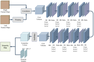
Dense Matching. At the lowest level, we follow the previous methods and build a full cost volume for disparity regression [17, 5]. It takes up little computation resources due to the negligible size of search space. We also use cost regularization to rectify the cost volume before the disparity regression with softmax. The cost regularization is composed of eight 3D convolutions all following a batch normalization layer. For the specific architecture please refer to the supplementary materials.

Detail Loss Detection. We formulate $FA_{l}$ as details that would disappear in the low level. We use a binary mask $M_{FA}$ to represents the positions of lost details, which is computed by a network $\mathcal{F}_{\rm{DLD}}$ based on the square difference between $F_{l}$ and upsampled $F^{\prime}_{l-1}$:

$$M_{FA_{l}} =\mathcal{F}_{\rm{DLD}}((F_{l}-F^{\prime}_{l-1})^{2};\theta),$$ (11)

where $\theta$ is the parameter of network. The network is composed of three convolution operations and a sigmoid function, and its learning is guided by an unsupervised loss. The unsupervised loss $\mathcal{L}^{\rm{DLD}}_{l}$ is designed by maximizing the differences between $F_{l}$ and $F_{l-1}$ on $FA_{l}$ and forcing the sparsity of $FA_{l}$ :

$$\mathcal{L}^{\rm{DLD}}_{l} =\mid{FA}_{l}\mid-\alpha\frac{\sum_{(h,w)\in{FA}_{l}}\parallel F_{l}(h,w)-F^{\prime}_{l-1}(h,w)\parallel_{2}}{\mid{FA}_{l}\mid}.$$ (12)

Benefiting from unsupervised learning, we do not need additional data annotation for training.

Sparse Matching. After obtaining the fine-grained areas, our focus turns to how to conduct the sparse matching on the extracted $\{FA_{l}\}_{l=0}^{l=L}$. It is not suitable to use cost volume representation, as $FA_{l}$ is content-aware whose shape and size are dynamic but not fixed. Instead, we opt for a direct computation of the disparity map. Specifically, we compute the cost via cross-correlation:

$$C_{l}(h,w,d) =<\acute{F}_{l}(h,w),\grave{F}_{l}(h,w-d)>,$$ (13)

where $\acute{F}_{l}$ and $\grave{F}_{l}$ are the deep features from left and right views respectively, $(h,w)\in\acute{FA}_{l}$ and $(h,w-d)\in\grave{FA}_{l}$. We then use softmax to get the probability distribution:

$$P_{l}(h,w,d) =\frac{\mathrm{e}^{C_{l}(h,w,d)-C_{l}^{max}(h,w)}}{\sum_{d=0}\mathrm{e}^{C_{l}(h,w,d)-C_{l}^{max}(h,w)}},$$ (14)

$$C_{l}^{max}(h,w) =\mathop{\max}_{d}\ C_{l}(h,w,d).$$

And we regress the sparse disparity map over the computed probability distribution as

$$\hat{D}_{l}(h,w) =\sum_{d=0}P_{l}(h,w,d)*d.$$ (15)

Compared to the full matching, the sparse matching not only reduces the number of points on $\acute{A}_{l}$, but also eliminates a lot of redundant matching on $\grave{A}_{l}$. As for the specific equation of back propagation, please refer to the supplementary materials.

$\rm Fusion_{l=1}$			$\rm Fusion_{l=2}$			$\rm Fusion_{l=3}$			EPE
dynamic upsampling	disparity fusion	refinement	dynamic upsampling	disparity fusion	refinement	dynamic upsampling	disparity fusion	refinement
-	-	-	-	-	-	-	-	-	2.104
✓	-	-	-	-	-	-	-	-	2.086
✓	✓	-	-	-	-	-	-	-	2.039
✓	✓	✓	-	-	-	-	-	-	1.286
✓	✓	✓	✓	-	-	-	-	-	1.208
✓	✓	✓	✓	✓	-	-	-	-	1.205
✓	✓	✓	✓	✓	✓	-	-	-	0.954
✓	✓	✓	✓	✓	✓	✓	-	-	0.896
✓	✓	✓	✓	✓	✓	✓	✓	-	0.893
✓	✓	✓	✓	✓	✓	✓	✓	✓	0.842

Table 2: The influence of each component in the Fusion step obatined on the Scene Flow dataset. $\mathrm{Fusion}_{l}$ represents the Fusion step at level $l$.

	Dense Result	Fusion Result	Hard Fusion	Soft Fusion
1	3.919	3.173	3.087	2.039
2	4.965	4.134	1.624	1.205
3	4.245	3.918	1.010	0.893

Table 3: The illustration of upsampled dense result $D_{l}^{{}^{\prime}}$ and fusion result $\bar{D}_{l}$ on the non-occluded fine-grained areas, and the result from hard fusion and soft fusion. Experiments are conducted on the Scene Flow dataset.

3.3.2 Fusion

Disparity Upsampling. After obtaining $D_{0}$ and $\{\hat{D}_{l}\}_{l=1}^{l=L}$, we fuse them hierarchically to compute the final output disparity map at the highest level. At each level, we first upsample the dense disparity map from previous level $D_{l-1}$ to current level ${D}^{\prime}_{l}$ in a content-aware fashion [38]. The content-aware weights are learned through three convolution operations with the input of the left feature map $\acute{A}_{l}$ at the current level and the dense disparity map $D_{l-1}$ from the previous level.

Disparity Fusion. According to Eq. 7, we could model the fusion process as the union of a collection of sets, like the superposition of multiple images, which we call as hard fusion. However, such a hard fusion performs poorly in practice due to the influence of occlusion. The occlusion results in severe matching ambiguity in sparse matching, while fine-grained areas contain many edges that are easy to occur in occlusion. Therefore, we propose to fuse the sparse disparity map $\hat{D}_{l}$ and the upsampled dense disparity map ${D}^{\prime}_{l}$ via a learned mask, which we call as soft fusion. Specifically, we use a regression network to generate the soft mask $M_{l}$. The regression network contains three 2D convolution operations and a sigmoid activation function. The input of regression network is the concatenation of left features $\acute{F}_{l}$, upsampled dense disparity map ${D}^{\prime}_{l}$, sparse disparity map $\hat{D}_{l}$, mask of current fine-grained areas $M_{\acute{FA}_{l}}$ and robustness mask of sparse matching $\hat{V}_{l}$. The pixel-wise robustness is formulated as the variance in sparse matching:

$$\hat{V}_{l}(h,w) =\sum_{d=0}P_{l}(h,w,d)*(\hat{D}_{l}(h,w)-d)^{2},$$ (16)

where $(h,w)\in\acute{FA}_{l}$ and $(h,w-d)\in\grave{FA}_{l}$. The generation of soft mask via regression network $\mathcal{F}_{\rm{REG}}$ is then formulated as

$$M_{l}=\mathcal{F}_{\rm{REG}}(cat(\acute{F}_{l},{D}^{\prime}_{l},\hat{D}_{l},M_{\acute{FA}_{l}},\hat{V}_{l});\ \theta).$$ (17)

$\theta$ is the parameter of regression network and $cat(\cdot)$ is the concatenation operation. After obtaining the soft mask $M_{l}$, we compute the soft fusion of dense and sparse disparity map as

$$\bar{D}_{l} ={D}^{\prime}_{l}(1-M_{l})+\hat{D}_{l}M_{l}.$$ (18)

Refinement. We further propose a refinement network to improve the sub-pixel accuracy of current dense disparity map $\bar{D}_{L}$. Specifically, we use $\bar{D}_{L}$ to warp the right feature maps. Then, we concatenate the warped right feature maps $\grave{F}^{\prime}_{l}$, left feature maps $\acute{F}_{l}$ and current disparity map $\bar{D}_{l}$ to feed into a refinement network $\mathcal{F}_{\rm{REF}}$ :

$$D_{l}=\bar{D}_{l}+\mathcal{F}_{\rm{REF}}(cat(\grave{F}^{\prime}_{l},\acute{F}_{l},\bar{D}_{l});\ \theta).$$ (19)

$\theta$ is the parameter of the refinement network, The refinement network contains seven convolution operations. All convolutions are followed by a relu activation function and a batch normalization level, except the last convolution that is only followed by a batch normalization level.

Figure 3: The visualization of results from detail loss detection and soft mask. The white areas in the second to last columns represent occlusion. The red points in the third and fourth columns represent the lost details, while the red points in the last two columns represent the learned soft mask.

4 Experiment

In this section, we conduct the most analysis of our model based on the Scene Flow dataset [23], except the complexity analysis which is carried out on the high-resolution Middlebury-v3 [34]. We also compare our model with state-of-the-art methods [23, 17, 5, 18, 37, 48, 41, 8, 1, 40, 42] based on Scene Flow [23], KITTI 2015 [24, 25, 26], and Middlebury-v3 [34].

We train our model end-to-end using Adam optimization with $\beta_{1}=0.9$, $\beta_{2}=0.999$ and batch size of $18$ on 3 Nvidia 1080Ti GPUs. We set the maximum of disparity as $216$ and apply color normalization to each input image during training. For the Scene Flow dataset, we train our model for 20 epochs with a learning rate of 0.001 which is then decayed by half every 7 epochs. For KITTI 2015 dataset, we fine-tune the model on mixed KITTI 2012 and KITTI 2015 training sets for 500 epochs. The initial learning rate is set as 0.001 and is decreased by half every 100 epochs after the 200th epoch. As for Middlebury-v3, we fine-tune the model pre-trained on Scene Flow. The learning rate is set to 0.001 for 300 epochs and then changed to 0.0001 for the rest of 600 epochs.

4.1 Analysis

4.1.1 Complexity Analysis

We analyze the complexity of our model by comparing the growth rate in computation cost with state-of-the-art methods. In order to obtain the curve of growth rate, we resize the image in Middlebury-v3, like the image named Australia, to obtain a sequence of inputs with different resolutions. We then test the running time of each method with the official code. The testing is conducted on a 1080Ti GPU with Cuda synchronization. As shown in Figure 1, most methods stop working on the high-resolution image due to the unaffordable memory consumption, while our method can still run on the image with $5000\times 3500$ resolution. The time cost of most state-of-the-art methods also grows exponentially when resolution increasing. Different from them, our model has a very low growth rate of time cost benefiting from our decomposition of stereo matching.

Models	EPE	$\rm>3px$	Time (ms)	Mem. (GB)
GA-Net-15 [48]	0.84	-	$4055^{*}$	$6.2^{*}$
Bi3D [1]	0.73	-	$1302^{*}$	$10.7^{*}$
GCNet [17]	2.51	9.34	950	-
PSMNet [5]	1.09	4.14	$640^{*}$	$6.8^{*}$
Waveletstereo [42]	0.84	4.13	270	-
AANet [40]	0.87	-	$147^{*}$	$1.2^{*}$
Deepruner-fast [8]	0.97	-	$87^{*}$	$1.9^{*}$
DispNetC [23]	1.68	9.31	60	-
StereoNet [18]	1.10	-	15	-
ours	0.84	3.58	50	1.6

Table 4: The comparison of algorithms on the Scene Flow dataset. ^∗ represents the result obtained on our machine with official code after Cuda synchronization in a unified setting. $EPE$ is the mean absolute disparity error in pixels. $>3px$ is the number of pixels whose predicted disparity is deviated from their ground truth by at least 3 pixels.

Comparing to the high-performing methods, GANet [48], our model is 100 times faster. Compared to the PSMNet [5], our model achieves almost $15\times$ speed increase. As for the DeepPruner [8], we still achieve almost twice faster running speed and better performance on memory consumption, even current implementation using a fixed-size level of decomposition. According to the theorem 10, our model could achieve better speed and memory consumption with a dynamic or larger size of decomposition.

Models	Noc			All			Time (ms)
	D1-bg	D1-fg	D1-all	D1-bg	D1-fg	D1-all
GCNet [17]	2.02	3.12	2.45	2.21	6.16	2.87	900
Bi3D [1]	1.79	3.11	2.01	1.95	3.48	2.21	480
PSMNet [5]	1.71	4.31	2.14	1.86	4.62	2.32	410
GA-Net-15 [48]	1.40	3.37	1.73	1.55	3.82	1.93	360
Waveletstereo [42]	2.04	4.32	2.42	2.24	4.62	2.63	270
HSM [41]	1.63	3.40	1.92	1.80	3.85	2.14	140
HD3S [44]	1.56	3.43	1.87	1.70	3.63	2.02	140
DispNetC [23]	4.11	3.72	4.05	4.32	4.41	4.34	60
Deepruner-fast [8]	2.13	3.43	2.35	2.32	3.91	2.59	60
AANet [40]	1.80	4.93	2.32	1.99	5.39	2.55	60
MADNet [37]	3.45	8.41	4.27	3.75	9.2	4.66	20
StereoNet [18]	-	-	-	4.3	7.45	4.83	15
ours	1.89	3.53	2.16	2.07	3.87	2.37	50

Table 5: The comparison of algorithms on the KITTI 2015 dataset. D1 metric measures the percentage of disparity outliers that exceed 3 pixels and $5\%$ of its true value. (Note: the time presented here are not tested in a unified setting. For fair comparison, please refer to the Table 4 and Figure 1).

Figure 4: The visualization of results on Middlebury-v3.

4.1.2 Ablation Study

We evaluate our model with different configurations to understand the effectiveness/influence of each component in our model. We use bicubic upsampling to upsample the prediction and compute the end-to-end point (EPE) with ground truth. As illustrated in Table 2, the error rate is reduced a little after using content-aware upsampling. The error rate is also improved after fusing the sparse results at each level. However, improvement is little. It is because the EPE metric in this table is calculated on the whole spatial space while the sparse result only improves a little area at each level $l$. Thus, we present the differences between upsampled dense result $D_{l}^{{}^{\prime}}$ and fusion result $\bar{D}_{l}$ only on the non-occluded fine-grained areas at each level $l$. As shown in Table 3, the fusion result $\bar{D}_{l}$ is better than the dense result $D_{l}^{{}^{\prime}}$, which mirrors the necessity of considering the lost details caused by downsampling. Furthermore, we compare the results from hard fusion and soft fusion to illustrate the necessity of considering the occlusion problem. As shown in Table 3, the soft fusion is much better than hard fusion at all levels. Furthermore, we analyze the effectiveness of our refinement network. As shown in Table 2, the performance is significantly improved with the refinement network.

4.1.3 Visualizing Results of Detail Loss Detection

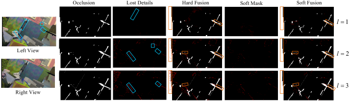
The goal of detail loss detection is to find the fine-grained areas at each scale. We visualize the learned binary mask to understand the efficacy of the detector. As shown in Figure 3, the thin or small objects are detected at a corresponding level $l$, especially in the blue boxes of the first and third columns.

4.1.4 Visualization of Soft Mask

We compare the visualization of hard fusion, soft mask, and soft fusion to understand the efficacy of soft fusion. As illustrated in Figure 3, most non-robust points, like the occluded points, are eliminated after soft fusion, especially in the orange boxes. We also find that the average value in soft attention is getting smaller when increasing the resolution. We think it is due to the reduced context of sparse matching, which deserves feature exploration, like dense graph net or transformer for better context learning in sparse matching.

4.2 Benchmark performance

SceneFlow. Following previous methods [8, 40], we split the state-of-the-art methods into two parts according to the running time whether exceeds 100ms. It also should be noted that the time and memory cost of some methods are obtained on our 1080Ti GPU with corresponding official code after Cuda synchronization for a fair comparision. As shown in Table 4, our method achieves comparable results among all the methods. Comparing to the high-performing method, our model reduces the cost of time and memory by order of magnitude while still achieving comparable results. We also provide qualitative results in supplementary materials to show the estimation of our model in different areas, like thin or small objects and large texture-less areas.

KITTI 2015. In KITTI 2015 dataset, as shown in Table 5, the time cost of reference methods is obtained from the official declaration, which means the different types of GPU and the possibility of Cuda synchronization not being used. As presented in Table 5, our model achieves comparable results and a significant improvement in complexity comparing to the high-performing methods. As for the methods with a running time less than 100ms, we achieve state-of-the-art results. We also provide some visualization in supplementary materials to show the competitive estimation of our model in various scenarios.

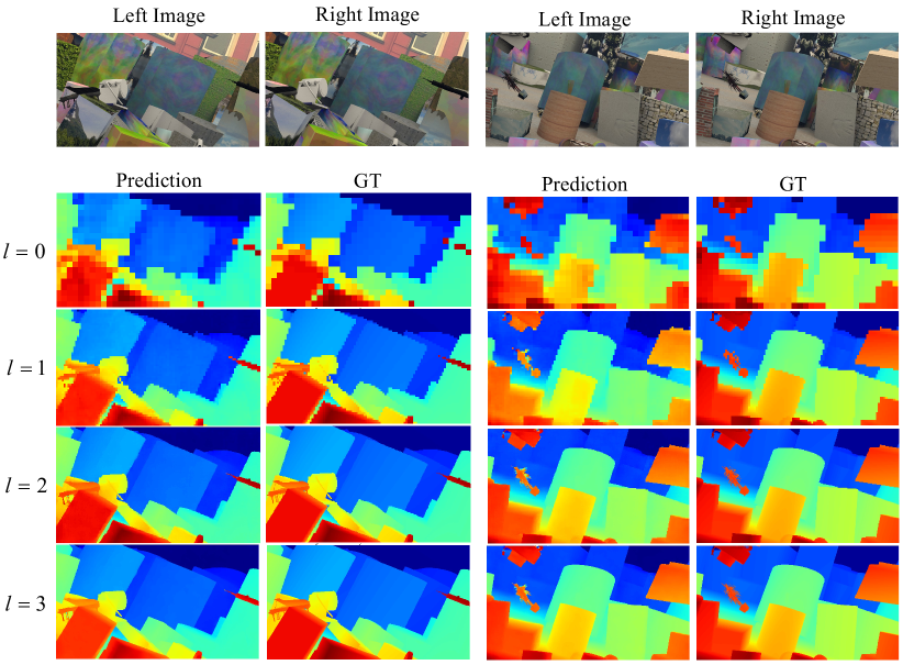
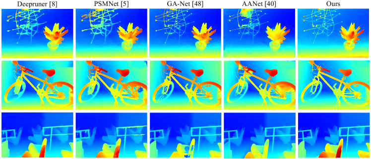
Middlebury-v3. In Middlebury-v3, we estimate the disparities based on the full-resolution inputs when most methods can only afford half resolution. Three examples are visualized in Figure 4 to show the ability of our model on the high-resolution image. For more results please refer to the supplementary materials.

5 Conclusion

In this paper, we have proposed a decomposition model for stereo matching. Compared with many state-of-the-art methods that face the problem of excessive growth in computational cost as the resolution increases, our model can reduce the growth rate by several orders of magnitude. Through a reference implementation of the modules in our model, we achieved state-of-the-art performance among real-time methods, and comparable results among high-performance methods with much lower cost on time and memory. Our model presents a new pipeline for the research of stereo matching, and state-of-the-art methods could be integrated into each step in our model to build a more powerful stereo matching method in the future.

6 Acknowledgment

This work was supported by the Natural Science Foundation of China (NSFC) under Grant No. 61773062.

Appendix A Method Details

A.1 Proof of Theorem 1

Theorem 1.

Supposing $s\in\{2,3,\cdots\}$ is the size of upsampling ratio between adjacent levels, $1<C\leq 8/7$ is a constant value and $\mathcal{O}(\cdot)$ represents the tight upper bound, then the complexity $\mathrm{O}$ of exhaustive search process is

$$\mathrm{O} =\mathrm{W}_{0}\mathrm{H}_{0}\mathrm{D}_{0}\ \mathcal{O}(s^{3L}C).$$ (20)

Proof.

As $\mathrm{W}_{l}=\mathrm{W}_{0}s^{l}$ and so does $\mathrm{H}_{l}$ and $\mathrm{D}_{l}$, we get $\mathrm{O}_{l}=\mathrm{W}_{l}\mathrm{H}_{l}\mathrm{D}_{l}=\mathrm{O}_{0}s^{3l}$. We then rewrite $\mathrm{O}=\sum_{l=0}^{l=L}\mathrm{O}_{l}$ as $\mathrm{O}=\sum_{l=0}^{L}\mathrm{O}_{0}s^{3l}=\mathrm{O}_{0}\frac{s^{3(L+1)}-1}{s^{3}-1}<\mathrm{O}_{0}s^{3L}\frac{s^{3}}{s^{3}-1}$. We use $C$ to represent $\frac{s^{3}}{s^{3}-1}$ where $1<\frac{s^{3}}{s^{3}-1}\leq\frac{8}{7}$ because $s$ is at least $2$. ∎

Figure 1: Architecture Of dense matching module. $3\times 3\times 3$ is the kernel size of 3D convolution, and $1\times 1\times 1$ is the stride size.

A.2 Dense Matching

As shown in Figure 1, we build the full cost volume via cross-correlation after warping the right feature maps. We then incorporate eright 3D convolutions to rectify the cost volume. A softmax operation is also used to turn cost volume into a probability volume. The dense disparity map is finally obtained via the regression of probability volume and the sampled disparities.

Models	Res	time (s)	time/MP (s)	time/GD (s)	NonOcc						All
					bad 2.0	bad 4.0	avgerr	rms	A90	A99	bad 2.0	bad 4.0	avgerr	rms	A90	A99
PSMNet [5]	Q	0.64	2.62	32.2	42.1	23.5	6.68	19.4	17.0	84.5	47.2	29.2	8.78	23.3	22.8	106
DeepPruner [8]	Q	0.13	0.41	4.38	30.1	15.9	4.80	14.7	10.4	67.7	36.4	21.9	6.56	18.0	17.9	83.7
GANet [48]	H	8.53	6.33	16.4	18.9	11.2	12.2	35.4	40.0	84.5	24.9	16.3	15.8	42.0	50.9	194
AANet [40]	H	4.56	4.17	11.0	25.2	19.6	8.88	26.2	24.2	131	31.8	25.8	12.8	32.8	41.4	142
ours	F	0.51	0.10	0.23	20.2	11.2	3.72	12.5	10.1	46.8	27.0	17.0	5.37	15.9	15.0	72.2

Table 1: The comparison of algorithms on Middlebury-v3 dataset (Q: quadratic resolution, H: half resolution, F: full resolution).

A.3 Backpropagation of Sparse Matching

In the main draft, sparse matching is formulated as follows:

$$C_{l}(h,w,d)=<\acute{F}_{l}(h,w),\grave{F}_{l}(h,w-d)>,$$ (21)

$$P_{l}(h,w,d) =\frac{\mathrm{e}^{C_{l}(h,w,d)-C_{l}^{max}(h,w)}}{\sum_{d=0}\mathrm{e}^{C_{l}(h,w,d)-C_{l}^{\max}(h,w)}},$$ (22)

$$C_{l}^{\max}(h,w) =\max_{d}C_{l}(h,w,d),$$

$$\hat{D}_{l}(h,w)=\sum_{d=0}P_{l}(h,w,d)\cdot d.$$ (23)

For the convenience of the derivation of the backpropagation, we rewrite the above equations as

$$\hat{D}_{l}(h,w)=\frac{\sum_{d=0}\mathrm{e}^{<}\acute{F}_{l}(h,w),\grave{F}_{l}(h,w-d)>-C_{l}^{\max}(h,w)\cdot d}{\sum_{d=0}\mathrm{e}^{<\acute{F}_{l}(h,w),\grave{F}_{l}(h,w-d)>-C_{i}^{\max}(h,w)}}.$$ (24)

We then compute the backpropagation over $\acute{F}_{l}(h,w)$ as

$$\frac{\partial\hat{D}_{l}(h,w)}{\partial\hat{F}_{l}(h,w,c)}=\sum_{d=0}( \hat{F}_{l}(h,w-d,c)(d-\hat{D}_{l}(h,w)$$ (25)

$$\mathrm{e}^{<\acute{F}_{l}(h,w),\grave{F}_{l}(h,w-d)>-C_{i}^{\max}(h,w)})$$

$$/\sum_{d=0} \mathrm{e}^{<\acute{F}_{l}(h,w),\grave{F}_{l}(h,w-d)>-C_{i}^{\max}(h,w)},$$

$$\frac{\partial\mathcal{L}}{\partial\dot{F}_{l}(h,w,c)}=\frac{\partial\mathcal{L}}{\partial\hat{D}_{l}(h,w)}\frac{\partial\hat{D}_{l}(h,w)}{\partial\dot{F}_{l}(h,w,c)}.$$ (26)

As for $\grave{F}_{l}(h,w)$, we compute its backpropagation as

$$\frac{\partial\hat{D}_{l}(h,w+d^{\prime})}{\partial\grave{F}_{l}(h,w,c)}= (\acute{F}_{l}(h,w+d^{\prime},c)(d^{\prime}-\hat{D}_{l}(h,w+d^{\prime})$$ (27)

$$\mathrm{e}^{<\acute{F}_{l}(h,w+d^{\prime}),\grave{F}_{l}(h,w)>-C_{i}^{\max}(h,w+d^{\prime})})$$

$$/\sum_{d=0}\mathrm{e}^{<\acute{F}_{l}(h,w+d^{\prime}),\grave{F}_{l}(h,w+d^{\prime}-d)>-C_{i}^{\max}(h,w+d^{\prime})}).$$

$$\frac{\partial\mathcal{L}}{\partial\grave{F}_{l}(h,w,c)}=\sum_{d^{\prime}=0}\frac{\partial\mathcal{L}}{\partial\hat{D}_{l}\left(h,w+d^{\prime}\right)}\frac{\partial\hat{D}_{l}\left(h,w+d^{\prime}\right)}{\partial\grave{F}_{l}(h,w,c)}$$ (28)

A.4 Loss

In addition to the unsupervised loss $\mathcal{L}^{\rm{DLD}}_{l}$ for detail loss detection, we also design a supervised loss for disparity estimation. As there is only ground truth $GT$ of disparity map at the highest level, we downsample the ground truth to each level $GT_{l}$. At the lowest level, we use smooth L1 between the predicted dense disparity map and the downsampled ground truth:

$$\mathcal{L}_{0} =smooth_{L_{1}}(\mathrm{D}_{0}-GT_{0}),$$ (29)

$$smoot\mathrm{H}_{L_{1}}(\epsilon) =\left\{\begin{array}[]{lr}0.5\epsilon^{2},&if\mid\epsilon\mid<1\\ \mid\epsilon\mid-0.5,&otherwise\end{array}\right..$$

At higher levels, there are four intermediate results at each level, including the upsampled dense disparity map from previous level ${D}^{\prime}_{l}$, the sparse disparity map $\hat{D}_{l}$, the fused disparity map $\bar{D}_{l}$ and the refined disparity map $\mathrm{D}_{l}$. To this end, we use a weighted combination of smooth L1 loss over them:

$$\mathcal{L}_{l}= \ \ \gamma_{1}*smooth_{L_{1}}(\mathrm{D}_{l}-GT_{l})$$ (30)

$$+\gamma_{2}*smooth_{L_{1}}(\bar{D}_{l}-GT_{l})$$

$$+\gamma_{3}*smooth_{L_{1}}(\hat{D}_{l}-GT_{l}\ M_{\acute{FA}_{l}})$$

$$+\gamma_{4}*smooth_{L_{1}}({D}^{\prime}_{l}-GT_{l}).$$

Finally, we train our model using end-to-end learning with following loss function:

$$\mathcal{L}=\mathcal{L}_{0}\cdot\mathrm{W}_{0}+\sum^{l=L}_{l=1}(\mathcal{L}_{l}\cdot\mathrm{W}_{l}+\mathcal{L}^{\rm{DLD}}_{l}w^{\prime}_{l}),$$ (31)

where $\mathrm{W}_{l}$ and $w^{\prime}_{l}$ are the loss weight.

Appendix B More Details on Experiment

We set $\gamma_{1}=0.5$, $\gamma_{2}=0.2$, $\gamma_{3}=0.2$, $\gamma_{4}=0.1$, and $w_{0}=0.037$, $w_{1}=0.11$, $w_{2}=0.33$, $w_{3}=1$, $w_{1}^{\prime}=0.01$.

B.1 Middlebury-v3

We present the comparison of results on the Middleburyv3 dataset [34]. We first give a brief description of the metric. time/MP: time normalized by the number of pixels (sec/megapixels). time/GD: time normalized by the number of disparity hypotheses (sec/(gigapixels*ndisp)). bad xx: percentage of ”bad” pixels whose error is greater than xx. avgerr: average absolute error in pixels. rms: root mean-square disparity error in pixels. Axx: xx-percent error quantile in pixels. As shown in Table 1, our model achieves the best speed on time/MP and time/GD. our model also obtains almost the best results on most metrics about accuracy.

B.2 KITTI 2015

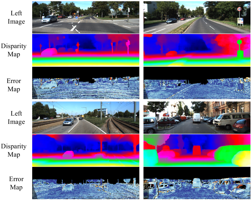
Despite the comparison with state-of-the-art methods in the main draft, we also give a visualization of our results on the KITTI 2015 dataset [24, 25, 26]. As shown in Figure 2, our model achieves competitive estimations in various scenarios.

Figure 2: Visualization of results on KITTI2015 dataset.

B.3 SceneFlow

We give a visualization of our results on the Scene Flow dataset [23]. As shown in Figure 3, our model achieves great results in different areas, like thin or small objects and large texture-less areas.

Figure 3: Visualization of results on Scene Flow dataset.

References

- [1] Badki. Bi3d: Stereo depth estimation via binary classifications. In Proceedings of the IEEE Conference on Computer Vision and Pattern Recognition (CVPR), pages 1600–1608, 2020.
- [2] Birchfield. Depth discontinuities by pixel-to-pixel stereo. International Journal of Computer Vision (IJCV), 35(3):269–293, 1999.
- [3] Bleyer. Patchmatch stereo-stereo matching with slanted support windows. In Proceedings of the British Machine Vision Conference (BMVC), volume 11, pages 1–11, 2011.
- [4] Boykov. Fast approximate energy minimization via graph cuts. IEEE Transactions on Pattern Analysis and Machine Intelligence (TPAMI), 23(11):1222–1239, 2001.
- [5] Chang. Pyramid stereo matching network. In Proceedings of the IEEE Conference on Computer Vision and Pattern Recognition (CVPR), pages 5410–5418, 2018.
- [6] Chen. Point-based multi-view stereo network. In Proceedings of the IEEE International Conference on Computer Vision (ICCV), pages 1538–1547, 2019.
- [7] Cheng. Deep stereo using adaptive thin volume representation with uncertainty awareness. In Proceedings of the IEEE Conference on Computer Vision and Pattern Recognition (CVPR), pages 2524–2534, 2020.
- [8] Duggal. Deeppruner: Learning efficient stereo matching via differentiable patchmatch. In Proceedings of the IEEE International Conference on Computer Vision (ICCV), pages 4384–4393, 2019.
- [9] Falkenhagen. Hierarchical block-based disparity estimation considering neighbourhood constraints. In International Workshop on Snhc and 3D Imaging, pages 115–122, 1997.
- [10] Geiger. Efficient large-scale stereo matching. In Proceedings of the Asian Conference on Computer Vision (ACCV), pages 25–38. Springer, 2010.
- [11] Gu. Cascade cost volume for high-resolution multi-view stereo and stereo matching. In Proceedings of the IEEE Conference on Computer Vision and Pattern Recognition (CVPR), pages 2495–2504, 2020.
- [12] He. Computing nearest-neighbor fields via propagation-assisted kd-trees. In IEEE Conference on Computer Vision and Pattern Recognition, pages 111–118. IEEE, 2012.
- [13] Hirschmüller. Real-time correlation-based stereo vision with reduced border errors. International Journal of Computer Vision (IJCV), 47(1-3):229–246, 2002.
- [14] Hirschmuller. Accurate and efficient stereo processing by semi-global matching and mutual information. In IEEE Computer Society Conference on Computer Vision and Pattern Recognition (CVPR), volume 2, pages 807–814. IEEE, 2005.
- [15] Hirschmuller. Stereo processing by semiglobal matching and mutual information. IEEE Transactions on Pattern Analysis and Machine Intelligence (TPAMI), 30(2):328–341, 2008.
- [16] Julesz. Foundations of cyclopean perception. 1971.
- [17] Kendall. End-to-end learning of geometry and context for deep stereo regression. In Proceedings of the IEEE International Conference on Computer Vision (ICCV), pages 66–75, 2017.
- [18] Khamis. Stereonet: Guided hierarchical refinement for real-time edge-aware depth prediction. In Proceedings of the European Conference on Computer Vision (ECCV), pages 573–590, 2018.
- [19] Kolmogorov. Computing visual correspondence with occlusions using graph cuts. In Proceedings of the IEEE International Conference on Computer Vision (ICCV), volume 2, pages 508–515. IEEE, 2001.
- [20] Liu. A novel recurrent encoder-decoder structure for large-scale multi-view stereo reconstruction from an open aerial dataset. In Proceedings of the IEEE Conference on Computer Vision and Pattern Recognition (CVPR), pages 6050–6059, 2020.
- [21] Lu. Patch match filter: Efficient edge-aware filtering meets randomized search for fast correspondence field estimation. In Proceedings of the IEEE Conference on Computer Vision and Pattern Recognition (CVPR), pages 1854–1861, 2013.
- [22] Marr. A computational theory of human stereo vision. Proceedings of the Royal Society of London. Series B. Biological Sciences, 204(1156):301–328, 1979.
- [23] Mayer. A large dataset to train convolutional networks for disparity. In Proceedings of the IEEE Conference on Computer Vision and Pattern Recognition (CVPR), pages 4040–4048, 2016.
- [24] Menze. Object scene flow for autonomous vehicles. In Proceedings of the IEEE Conference on Computer Vision and Pattern Recognition (CVPR), pages 3061–3070, 2015.
- [25] Moritz Menze, Christian Heipke, and Andreas Geiger. Joint 3d estimation of vehicles and scene flow. In Isprs Workshop on Image Sequence Analysis (ISA), 2015.
- [26] Moritz Menze, Christian Heipke, and Andreas Geiger. Object scene flow. Isprs Journal of Photogrammetry and Remote Sensing (JPRS), 2018.
- [27] Min. Cost aggregation and occlusion handling with wls in stereo matching. IEEE Transactions on Image Processing (TIP), 17(8):1431–1442, 2008.
- [28] Min. A revisit to cost aggregation in stereo matching: How far can we reduce its computational redundancy? In Proceedings of the IEEE International Conference on Computer Vision (ICCV), pages 1567–1574. IEEE, 2011.
- [29] Von Noorden. Binocular vision and ocular motility. Theory and Management of Strabismus, 1990.
- [30] Ogle. Researches in binocular vision. 1950.
- [31] Richardt. Real-time spatiotemporal stereo matching using the dual-cross-bilateral grid. In Proceedings of the European Conference on Computer Vision (ECCV), pages 510–523. Springer, 2010.
- [32] Ronneberger. U-net: Convolutional networks for biomedical image segmentation. In Proceedings of the International Conference on Medical Image Computing and Computer-Assisted Intervention, pages 234–241. Springer, 2015.
- [33] Scharstein. A taxonomy and evaluation of dense two-frame stereo correspondence algorithms. International Journal of Computer Vision (IJCV), 47(1-3):7–42, 2002.
- [34] Scharstein. High-resolution stereo datasets with subpixel-accurate ground truth. In Proceedings of the German Conference on Pattern Recognition (GCPR), pages 31–42, 2014.
- [35] Sinha. Efficient high-resolution stereo matching using local plane sweeps. In Proceedings of the IEEE Conference on Computer Vision and Pattern Recognition (CVPR), pages 1582–1589, 2014.
- [36] Sun. Stereo matching using belief propagation. IEEE Transactions on Pattern Analysis and Machine Intelligence (TPAMI), 25(7):787–800, 2003.
- [37] Tonioni. Real-time self-adaptive deep stereo. In Proceedings of the IEEE Conference on Computer Vision and Pattern Recognition (CVPR), pages 195–204, 2019.
- [38] Wang. Carafe: Content-aware reassembly of features. In Proceedings of the IEEE International Conference on Computer Vision (ICCV), 2019.
- [39] Wheatstone. Xviii. contributions to the physiology of vision.—part the first. on some remarkable. Philosophical Transactions of the Royal Society of London, (128):371–394, 1838.
- [40] Xu. Aanet: Adaptive aggregation network for efficient stereo matching. In Proceedings of the IEEE Conference on Computer Vision and Pattern Recognition (CVPR), pages 1959–1968, 2020.
- [41] Yang. Hierarchical deep stereo matching on high-resolution images. In Proceedings of the IEEE Conference on Computer Vision and Pattern Recognition (CVPR), pages 5515–5524, 2019.
- [42] Yang. Waveletstereo: Learning wavelet coefficients of disparity map in stereo matching. In Proceedings of the IEEE Conference on Computer Vision and Pattern Recognition (CVPR), pages 12885–12894, 2020.
- [43] Yao. Recurrent mvsnet for high-resolution multi-view stereo depth inference. In Proceedings of the IEEE Conference on Computer Vision and Pattern Recognition (CVPR), pages 5525–5534, 2019.
- [44] Yin. Hierarchical discrete distribution decomposition for match density estimation. In Proceedings of the IEEE Conference on Computer Vision and Pattern Recognition (CVPR), pages 6044–6053, 2019.
- [45] Yoon. Adaptive support-weight approach for correspondence search. IEEE Transactions on Pattern Analysis and Machine Intelligence (TPAMI), 28(4):650–656, 2006.
- [46] Yu. Fast-mvsnet: Sparse-to-dense multi-view stereo with learned propagation and gauss-newton refinement. In Proceedings of the IEEE Conference on Computer Vision and Pattern Recognition (CVPR), pages 1949–1958, 2020.
- [47] Zbontar. Computing the stereo matching cost with a convolutional neural network. In Proceedings of the IEEE Conference on Computer Vision and Pattern Recognition (CVPR), pages 1592–1599, 2015.
- [48] Zhang. Ga-net: Guided aggregation net for end-to-end stereo matching. In Proceedings of the IEEE Conference on Computer Vision and Pattern Recognition (CVPR), pages 185–194, 2019.