FedSAE: A Novel Self-Adaptive Federated Learning Framework in Heterogeneous Systems

Abstract

Federated Learning (FL) is a novel distributed machine learning which allows thousands of edge devices to train model locally without uploading data concentrically to the server. But since real federated settings are resource-constrained, FL is encountered with systems heterogeneity which causes a lot of stragglers directly and then leads to significantly accuracy reduction indirectly. To solve the problems caused by systems heterogeneity, we introduce a novel self-adaptive federated framework FedSAE which adjusts the training task of devices automatically and selects participants actively to alleviate the performance degradation. In this work, we

1) propose FedSAE which leverages the complete information of devices’ historical training tasks to predict the affordable training workloads for each device. In this way, FedSAE can estimate the reliability of each device and self-adaptively adjust the amount of training load per client in each round.

2) combine our framework with Active Learning to self-adaptively select participants. Then the framework accelerates the convergence of the global model. In our framework, the server evaluates devices’ value of training based on their training loss. Then the server selects those clients with bigger value for the global model to reduce communication overhead.

The experimental result indicates that in a highly heterogeneous system, FedSAE converges faster than FedAvg, the vanilla FL framework. Furthermore, FedSAE outperforms than FedAvg on several federated datasets — FedSAE improves test accuracy by $26.7\%$ and reduces stragglers by $90.3\%$ on average.

I Introduction

Federated Learning (FL) [1, 2, 3], famous for its significant contribution on privacy protection [4], is one of the most popular topics on distributed machine learning, widely used in personalized recommendation [5, 6] and clinical disease detection [7]. Similar to the traditional distributed machine learning framework, FL performs most of its computation on remote clients but no data sharing between clients and the server in the FL training procedure. Typical FL includes a central server and millions of remote clients such as personal computers, mobile phones, wearable devices, and so on. In each communication round, due to constraint network connectivity, the FL server only selects several participants which train a model such as neural networks locally, and then these participants upload their model parameters to the server periodically. Finally, the server aggregates these uploaded model parameters to get a new global model. Usually, to train an FL model, several training rounds are performed, during which no raw data leaves clients. This unique training mechanism keeps FL privacy-preserving compared with conventional distributed machine learning.

Nonetheless, a key challenge of FL is that the devices’ configurations such as GPU, CPU, software, and network conditions are markedly different in real federated settings. This challenge is called systems heterogeneity [3, 8] which causes the overhead of devices such as computation time and resources to accomplish the same task to vary heavily. Due to the different training overhead, some devices with high performance can complete their task. However, others called stragglers [10] with poor training conditions can only do partial training work, which leads to performance degradation of the global model. Unfortunately, to handle the problem of stragglers, the FL server can only choose to wait or ignore them [9] because devices take full control of the connection at each round. Systems heterogeneity heavily slows down the convergence rate and decreases the model accuracy [10] as the existence of numerous stragglers.

To solve the problem of systems heterogeneity, Nishio et al. [11] propose FedCS which selects devices with enough resources to participate in FL training. However, this method requests the server to gather the available resource information of clients, which violates the principle of privacy protection. To alleviate the negative influence of stragglers, Li et al. [10] propose FedProx which allows each device to perform a variable amount of local work to endure the partial work of stragglers. FedProx successfully promotes the test accuracy by 22% on average compared with FedAvg. However, FedProx assumes that the partial work which stragglers can finish is known before stragglers drop out, which is impractical in a real federated setting. Moreover, the occurrence of drop out is unpredictable which means stragglers can not upload their partial work before they drop out. In most FL frameworks, the server usually assigns the same training workload to all of the selected clients, which neglects systems heterogeneity hence causes the high probability of stragglers.

In this paper, we propose FedSAE, a self-adaptive FL framework aiming to alleviate the performance degradation caused by systems heterogeneity. In FedSAE, the server self-adaptively adjusts the workloads allocated to clients according to their training history. Meanwhile, to accelerate the model convergence speed, we propose a mechanism based on active learning to select clients, which improves the quality of the global model. We compare our framework with FedAvg [2] in highly heterogeneous networks. The experiment results convey that FedSAE improves the absolute testing accuracy by 26.7% and decreases the drop out rate by 90.3% on average.

The main contributions of this paper are as follows:

• We consider a new drop out scenario, which is more complex than the previous FL settings. In our work, the ability of clients to complete the training task is varied dynamically, so the probability of stragglers is also dynamic. Therefore, we propose a workload prediction algorithm for this heterogeneous scenario.

• We propose two federated algorithms, FedSAE-Ira and FedSAE-Fassa, to efficiently predict the affordable training workload of clients. Our methods are self-adaptive and privacy-preserving which works relying on the public training history of devices rather than any other private hardware information.

• We evaluate our methods with two models on four datasets. Comparing with baseline FedAvg, our methods significantly upgrade the accuracy of the global model by 26.7% and alleviate stragglers by 90.3%.

II background and related work

II-A Federated Learning

In this subsection, we introduce the classical FL algorithm FedAvg. And then, we briefly introduce systems heterogeneity.

Federated Averaging. Federated learning is introduced in [2] where McMahan et al. propose the classical FL algorithm FedAvg. In FedAvg, the server coordinates clients to perform stochastic gradient descent (SGD) locally several iterations in parallel and updates global model by aggregating the uploaded model parameters from clients with Federated Averaging (FedAvg)[2]. During the FL training process, no raw data but model weights are transmitted between clients and the server. Before FedAvg, pioneers rely on full-batch SGD to train the federated learning model. To get an optimal model, the server usually training hundreds of rounds which produces a large communication overhead. By utilizing the powerful computation ability of clients, FedAvg forces clients to perform local mini-batch SGD several times to reduce the communication rounds and is communication-efficient.

In FedAvg, the particular object function is to optimize [10]:

$$\min\limits_{{\bm{w}}}f(\bm{w})=\sum_{k=1}^{N}\frac{n_{k}}{n}F_{k}(\bm{w}),$$ (1)

Where $N$ is the number of total clients, $n$ is the total samples of $N$ clients i.e. $n=\sum_{k=1}^{N}n_{k}$, and $\frac{n_{k}}{n}$ is the weight of client $k$. For client $k$, the local objective function $F_{k}(\bm{w})$ is denoted by [10]:

$$F_{k}(\bm{w})=\frac{1}{n_{k}}\sum_{\bm{i}\in\mathcal{D}_{k}}f_{i}(\bm{w})$$ (2)

where $\mathcal{D}_{k}$ is the training data on client $k$. $f_{i}(\bm{w})=\ell_{i}(x_{i},y_{i};w)$ is the loss function on examples $(\bm{x},\bm{y})\in\mathcal{D}_{k}$. If $\mathcal{D}_{k}$ is sampled from global data uniformly, then $F_{k}(\bm{w})\approx f(\bm{w})$ holds approximatively. The approximation level between local objective and global objective improves as the increasing uniformity of client data $\mathcal{D}_{k}$. That is why FedAvg performs well on independently and identically distributed (IID) datasets.

In FedAvg, at each round $t$, the server selects $K$ clients randomly ($K=C*N$, $C$ is the selected ratio in $N$ clients) and broadcasts the initial model parameter $w^{t}$ to participants. The selected client (assumed client $k$) minimizes the local function loss $F_{k}(\bm{w})$ by performing SGD $E$ epochs locally (an epoch means training all the data on client $k$ once). At last, the server aggregates these parameters $w_{k}^{t+1}$ with federated averaging according to clients’ weight $\frac{n_{k}}{n}$ to get the global parameter $w^{t+1}$ of round $t+1$. In general, the above process is executed $T$ rounds, i.e. the number of communication rounds is $T$. The details of FedAvg is shown in Algorithm 1.

Algorithm 1 Federated Averaging (FedAvg)

1:initial model parameter $\bm{w}^{0}$, client fraction $C$, the number of clients $K$, the number of local epoch $E$, the learning rate $\eta$.

2:the eventual model parameter $\bm{w}$.

3:Initialize $\bm{w}^{0}$.

4:for each communication round t = 1,2,3,…,T do

5:    $S_{t}$ $\leftarrow$ (Server selects $C*K$ clients clients randomly)

6:    Server broadcasts model parameters $\bm{w}_{t}$ to $S_{t}$.

7:    for client $k\in S_{t}$ parallelly do

8:         //clients perform SGD locally

9:         for local epoch $e=1,2,3,...,E$ do

10:             $\bm{w}_{k}^{t+1}\leftarrow\bm{w}_{k}^{t}-\eta\nabla F_{k}(\bm{w}_{k}^{t})$          

11:         $\bm{w}^{t+1}\leftarrow\sum_{k=1}^{K}\frac{n_{k}}{n}\bm{w}_{k}^{t+1}$     

12:return $\bm{w}\leftarrow\bm{w}^{t+1}$

Systems heterogeneity. Systems heterogeneity is a challenge in FL [3]. It is inevitable because remote devices own varied configuration conditions such as GPU, CPU, memory, networks, etc. Due to systems heterogeneity, clients have different resource budgets thereby not all participants can finish their training tasks[10]. So some devices finish their training tasks fastly while some others called stragglers [10] train their model slowly even drop out. These devices with better resource conditions could finish their training task more possible. That is to say, systems heterogeneity causes heterogeneous training ability. Conventional FL methods solve this problem by waiting for stragglers or omitting them[2], which leads to the accuracy degradation of the global model and slows down model convergence. Our work in this paper is to solve the systems heterogeneity challenges.

II-B Related Work

Federated Learning. Based on the first work on FL algorithm FedAvg [2], the early FL studies are more about solving the statistical heterogeneity challenge in which the data distributed on devices is non-independent and non-identical (Non-IID). Zhao et al.[12] find that the accuracy of FedAvg decreases by 55% on highly skewed Non-IID datasets. Thereby [13, 12, 14] aim to enhance the accuracy of the global model on Non-IID data. At the same time, that the global model converges slowly is another problem caused by Non-IID data[10], which induces [15, 16] to make efforts on increasing the convergence rate of the global model, [17, 10, 18] to provide convergence guarantees for Non-IID data. Some pioneers work hard at reducing the communication overhead between clients and the server [1, 19, 20, 21, 22, 23]. For another aspect, some researchers try building a better FL system instead of optimizing the FL algorithm [24, 19, 9] where [9] preliminarily explores a scalable production FL system for Android while [24, 19] provide FL more secure privacy protection. However, the above works assume that all clients are equivalent in the training process, which causes a big performance variance in clients. Recently, some literature indicates that more fair local model performance distribution across clients contributes to a better global model [25, 26]. But the idea of performance fairness conflicts with privacy for the reason that it collects much sensitive information to ensure that the eventual distribution of local performance is fair enough.

Systems Heterogeneity and Straggling. Systems heterogeneity generally exists in a real federated environment and it slows down the convergence rate of model [3]. Heterogeneous systems usually lead to the straggle issue in FL. We can not eliminate systems heterogeneity but mitigate device straggling caused by it. Some works reduce stragglers by selecting clients with enough resources [11, 27]. Nishio et al. [11] propose FedCS which selects clients according to constrained time budget and resource budget to prevent participants from dropping out because of lack of resources [9]. But it is difficult to judge whether the resource is enough or not. Rahman et al. [27] propose another client selection framework FedMCCS which selects clients according to multi-criteria such as location, resource, etc. However, the strict constraints of client selection may cause few participants thus slow down the convergence. Instead of selecting clients conditionally, Li et al. [10] propose FedProx which utilizes the partial work of stragglers to alleviate the model performance degradation. But FedProx is too ideal to be implemented in real federated settings where whether a client will straggle is unknown. To avoid wasting the partial work of stragglers, Ferdinand et al. [28] propose Anytime Minibatch and Reisizadeh et al. [29] propose QuanTimed-DSGD. The two frameworks contribute to a novel training way that fixes the computation time of devices instead of fixing computation epochs.

III Federated Optimization: FedSAE

In this section, we describe the motivation of this paper and then introduce the details of the proposed method FedSAE.

III-A Motivation

Before introducing our framework, we conduct a simple experiment to show the motivation of this paper. To reveal the accuracy decrease of FedAvg in heterogeneous systems, we implement a convex multinomial logistic regression task training with FedAvg on MNIST [30] dataset and Federated Extend MNIST (FEMNIST) [31, 32] dataset.

For heterogeneous FL systems, a more reasonable design is to build a more complex federated environment, in which the client’s ability to perform training tasks changes dynamically. So we simulate a heterogeneous environment by varying the computing ability of each client with time separately. The affordable workload of each client is refreshed with a Gaussian Distribution in each round where the mean value $\mu$ is randomly initialized from the interval $[5,10)$, and the standard deviation $\sigma$ is randomly initialized from the interval $[0.25\mu,0.5\mu)$.

In our motivation experiment, we assign each client a varying amount of affordable local epoch each round, which quantifies the ability of clients to finish their training tasks. In the FEMNIST dataset, the number of clients is $N=200$, we set the number of selected clients $K=10$ per round. In MNIST dataset, $N=1000$, we set $K=30$. We set learning rate $\eta=0.03$ to train $T=200$ rounds with FedAvg and test the global model in each round. We run FedAvg on FEMNIST and MNIST four times with $epoch=10,12,15,20$ separately. The top-1 testing accuracy of the global model, training loss, and drop out rate of clients are depicted in Fig. 1.

From Fig. 1 we can see that taking the testing accuracy with $epoch=10$ as the reference accuracy, as the local epoch increases, the averaging testing accuracy on FEMNIST decreases by $5.2\%$ to $52.2\%$, and the average testing accuracy on MNIST decreases by $1.1\%$ to $53.3\%$. Also, we can see that as the local epoch increases, the training loss on the two datasets decreases more and more slowly. In extreme cases (i.e. $epoch=20$), the training loss even increases, which means that the training task fails because the model is diverging. Besides, we find that the drop out rate fluctuates greatly when $epoch>10$, and almost all clients drop out when $epoch=20$. This is because FedAvg cannot self-adapt the training task to the training ability of clients. In short, Fig. 1 shows that when FL systems are heterogeneous, the performance degradation of traditional FL framework (e.g. FedAvg) is very obvious.

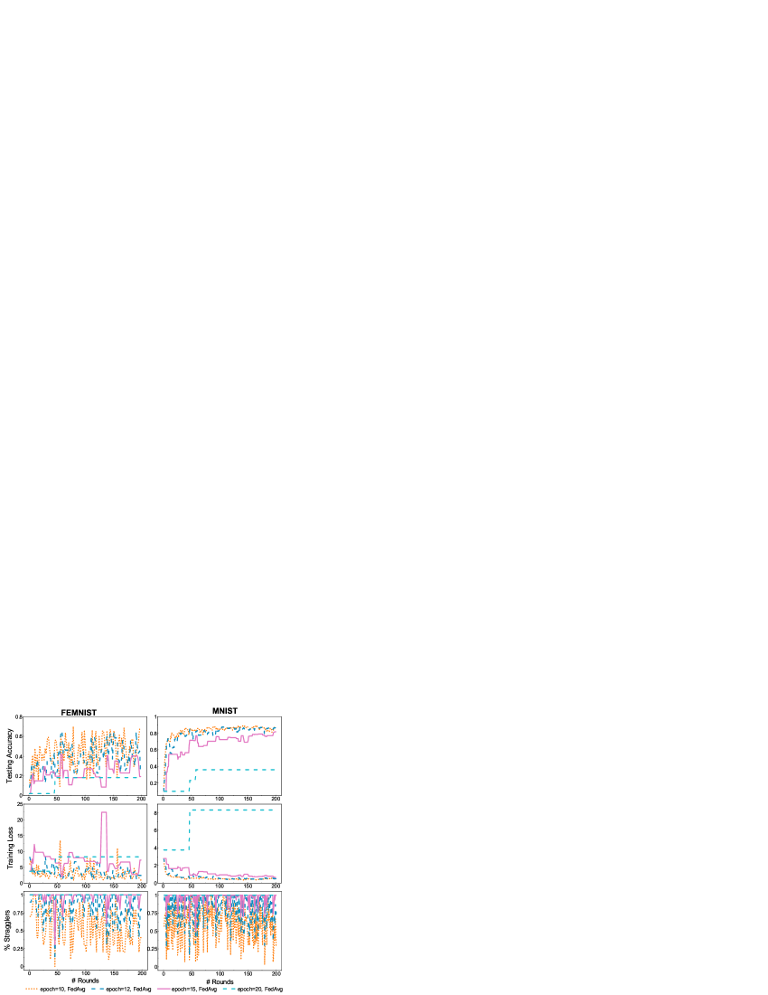
Figure 1: The results of FedAvg trained on FEMNIST and MNIST datasets. The real affordable local epoch of each client is varying while the training epoch allocated to clients is fixed (i.e. $epoch=10,12,15,20$). With allocated epoch increasing from 10 to 20, averaging testing accuracy reduces by up to 53.3% on MNIST, and the averaging drop out rate increases by up to 41% on FEMNIST, which means considering systems heterogeneity, the performance of FedAvg declines heavily. That’s because many clients do not finish their assignments.

III-B Proposed Framework: FedSAE

To handle systems heterogeneity challenges in FL, we propose a new FL framework, FedSAE which leverages workload prediction strategy based on the workload complete history of clients to predict the varied affordable workload of clients. Besides, FedSAE uses client selection strategy based on the training loss of clients to pick participants each round. Our framework is similar to FedAvg in the training process. Both of them include selecting clients, broadcasting models, locally performing SGD, uploading local models, and aggregating models. However, FedSAE has two changes: predicting affordable workload and selecting participants with active learning (AL). These changes make our framework more rational in practical federated settings. Before detailedly introducing our changes, we show our framework in Fig. 2.

As shown in Fig. 2, the training process of FedSAE can be divided into four steps. First, the server predicts the affordable workload of clients according to their uploaded historical task completion information (①). Second, the server converts clients’ training loss into selected probability (②). Third, the server picks participants according to probabilities in ② then broadcasts the global model and participants’ predicted workload to participants (③). At last, participants return model parameters, new task completion information and loss to the server and the server aggregates model weights for the next round (④). We will introduce ① and ② in detail in the rest of this section.

Affordable workload prediction. As we discussed before, the ability of clients to perform training tasks in a heterogeneous system is varied dynamically. Clients participating in training without self-adaptively adjusting the number of training workloads are more likely to drop out, which leads to an inefficient global model. Therefore, it is necessary to predict the affordable workload of clients correctly. To better predict the affordable workload of clients, FedSAE utilizes a task pair $(L_{k}^{t},H_{k}^{t})$ to limit the maximum and minimum values of affordable workload, where $L_{k}^{t}$ represents the amount of easy task, $H_{k}^{t}$ represents the amount of difficult task, obviously, $L_{k}^{t}\textless H_{k}^{t}$. Each client will maintain a task pair. The client first performs the easy workload $L_{k}^{t}$ and then increases its workload until it drops out or completes the difficult workload $H_{k}^{t}$. This pair is beneficial in two aspects: (1) It makes sure that devices at least finish a conservative workload $L_{k}^{t}$ instead of dropping out. (2) It predicts the affordable workload of clients to a specified range, which is more stable than directly accurate to the amount of affordable workload.

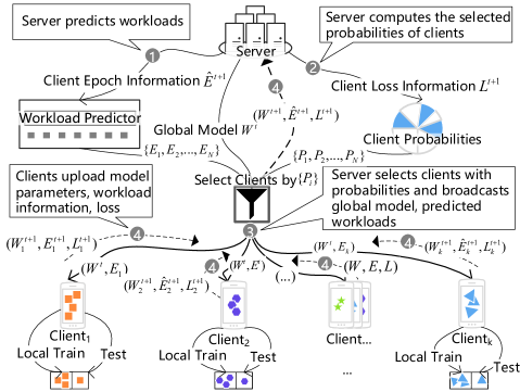
Figure 2: The workflow of FedSAE.

Considering the workload prediction task is similar to the congestion control task in communication technology, we get inspiration from classic TCP congestion control algorithms[33, 34]. We propose two algorithms—-FedSAE-Ira (Algorithm 2) and FedSAE-Fassa (Algorithm 3) to predict the affordable workload of clients according to the historical task completion information. For client $k$, it records $\tilde{E_{k}^{t}}$, the amount of workload it can accomplish recently, as the prediction basis of the workload prediction algorithms. Specifically, to predict the affordable workload of the next round, FedSAE-Ira utilizes clients’ task completion of the latest round while FedSAE-Fassa utilizes clients’ task completion of many past rounds. The details of the two algorithms are as follows:

Algorithm 2 FedSAE-Ira: Federated Self-Adaptive Epoch with inverse ratio arise (Proposed Framework)

1:the actually affordable local epoch $\tilde{E}_{k}^{t}$ of client $\bm{k}$ at round t, the server-predict workloads $\hat{E}_{k}^{t}$, the easy workloads $\hat{L}_{k}^{t}$, the difficult workloads $\hat{H}_{k}^{t}$.

2:the predicted easy workloads $\hat{L}_{k}^{t+1}$, the predicted difficult workloads $\hat{H}_{k}^{t+1}$.

3:procedure Server

4:    Initialize $\bm{w}^{0}$, $\hat{L}_{k}^{0}$, $\hat{H}_{k}^{0}$

5:    for each communication round $t=1,2,...,T$ do

6:        $S_{t}\leftarrow$ Select $K$ clients according to selected probabilities.

7:        Server broadcasts $\bm{w}_{t}$ to all selected clients.

8:        $(\hat{L}_{k}^{t},\hat{H}_{k}^{t},\tilde{E}_{k}^{t})\leftarrow$ Read history data from $S_{t}$.

9:        for each client $k\in S_{t}$ in parallel do do

10:           $(\hat{L}_{k}^{t+1},\hat{H}_{k}^{t+1},\hat{E}_{k}^{t})\leftarrow$ EpochPredict ($\hat{L}_{k}^{t}$, $\hat{H}_{k}^{t}$, $\tilde{E}_{k}^{t}$)

11:           ${w}_{k}^{t+1}\leftarrow$ Client($k$, $\bm{w}^{t}$, $\hat{E}_{k}^{t}$)         

12:        $\bm{w}^{t+1}\leftarrow\sum_{k=1}^{K}\frac{n_{k}}{n}\bm{w}_{k}^{t+1}$     

13:// run on server

14:function EpochPredict($\hat{L}_{k}^{t}$, $\hat{H}_{k}^{t}$, $\tilde{E}_{k}^{t}$) // client $\bm{k}$ will not drop out.

15:    if  the actual affordable workloads greater than $\hat{H}_{k}^{t}$ then

16:        $\hat{L}_{k}^{t+1},\hat{H}_{k}^{t+1}\leftarrow\hat{L}_{k}^{t}+\frac{\mathcal{U}}{\hat{L}_{k}^{t}},\hat{H}_{k}^{t}+\frac{\mathcal{U}}{\hat{H}_{k}^{t}}$

17:        $\hat{E}_{k}^{t}\leftarrow\hat{H}_{k}^{t}$ // client $\bm{k}$ will drop out but weight at epoch $\hat{L}_{k}^{t}$ will be uploaded.

18:    else if the actually affordable workloads fall into $[\hat{L}_{k}^{t},\hat{H}_{k}^{t}]$ then

19:        $\hat{L}_{k}^{t+1}\leftarrow min(\hat{L}_{k}^{t}+\frac{\mathcal{U}}{\hat{L}_{k}^{t}},\frac{1}{2}\hat{H}_{k}^{t})$

20:        $\hat{H}_{k}^{t+1}\leftarrow max(\hat{L}_{k}^{t}+\frac{\mathcal{U}}{\hat{L}_{k}^{t}},\frac{1}{2}\hat{H}_{k}^{t})$

21:        $\hat{E}_{k}^{t}\leftarrow\hat{L}_{k}^{t}$ // client k will drop out and no weight will be uploaded.

22:    else

23:        $\hat{L}_{k}^{t+1},\hat{H}_{k}^{t+1}\leftarrow\frac{1}{2}\hat{L}_{k}^{t},\frac{1}{2}\hat{H}_{k}^{t}$

24:        $\hat{E}_{k}^{t}\leftarrow 0$     

25:    return $\hat{L}_{k}^{t+1}$, $\hat{H}_{k}^{t+1}$, $\hat{E}_{k}^{t}$

26:// run on client $\bm{k}$

27:function Client($k$, $\bm{w^{t}}$, $\hat{E}_{k}^{t}$)

28:    $\mathcal{B}\leftarrow(seperate~{}\mathcal{P}_{k}~{}into~{}batches~{}of~{}size~{}B)$

29:    for each local epoch $e=1,2,...,\hat{E}_{k}^{t}$ do

30:        for each local batch $b\in\mathcal{B}$ do

31:           $\bm{w^{t}}\leftarrow\bm{w^{t}}-\eta\nabla L(b;\bm{w^{t}})$             

32:    return $\bm{w^{t}}$

III-B1 FedSAE-Ira

In Algorithm 2, we show the simple process of FedSAE-Ira in which the increased workload is inversely proportional to itself. If a client drops out, the client’s predicted workload of the next round will be half of the current round otherwise the predicted workload of the client will increase by increment $\frac{\mathcal{U}}{\hat{E}_{k}^{t}}$ (see the line 11 to line 22 in Algorithm 2). As shown in Fig. 3, at the beginning of the training the workload of clients is conservative and easy. Therefore, the workload increases fastly by increment $\frac{\mathcal{U}}{\hat{E}_{k}^{t}}$ which is inversely proportional to the amount of current workload until the client drops out in round $t$. And then, the workload of the client in round $t+1$ turns to half of the current workload. In this process, FedSAE-Ira shows the following advantages: (1) It is cautious to increase the workload of clients in a gradually smaller increment, which can reduce the drop out probability of clients to a certain extent. (2) It reduces workload exponentially after dropping out, which makes the workload recover to a safe level quickly. In this way, the client avoids dropping out consecutively.

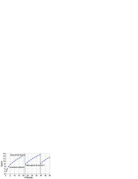
Figure 3: The simple process diagram of FedSAE-Ira. If the client drops out at round $t$, the predicted workload of the next round $t+1$ turns to be halved. If not, it keeps increasing in inverse proportion e.g. client $k$ at $t$-th round increased by $\frac{\mathcal{U}}{E_{k}^{t}}$.

We simply summarize the predicted workload of clients as the following equation:

$$\begin{split}\hat{E}_{k}^{t+1}=\left\{\begin{array}[]{ll}\frac{1}{2}\hat{E}_{k}^{t},&if~{}client~{}k~{}drops~{}out\\ \hat{E}_{k}^{t}+\frac{\mathcal{U}}{\hat{E}_{k}^{t}},&otherwise\end{array}\right.\end{split}$$ (3)

where $\hat{E}_{k}^{t}$ is the predicted workload of client $k$ in $t$-th round, $\mathcal{U}$ is the hyperparameter to control the increment. An appropriate $\mathcal{U}$ is efficient because an excessively high $\mathcal{U}$ makes the prediction process fluctuated while an excessively low $\mathcal{U}$ causes the time converging to the affordable workload interval too long. In FedSAE-Ira, $L_{k}^{t}$ and $H_{k}^{t}$ are predicted according to (3). This method is a kind of Additive Increase Multiplicative Decrease (AIMD) method[35] which is a feedback control algorithm with linear growth and exponential reduction. Chiu et al.[33] demonstrate that for an additive increase and multiplicative decrease iterative process, the method is convergent.

III-B2 FedSAE-Fassa

In order to make full use of the history of task completion, we propose FedSAE-Fassa which utilizes the amount of the affordable workload of many past rounds to self-adaptively predict the affordable workload of the next round. As shown in Algorithm 3, first, the server calculates the workload threshold $\theta_{k}^{t}$ of $k$-th client in round $t$ as (4) based on the historical workload records (see the line 8 in Algorithm 3). $\theta$ represents the number of workloads that the client can complete in most cases.

$$\theta_{k}^{t+1}=\alpha\theta_{k}^{t}+(1-\alpha)\tilde{E}_{k}^{t}$$ (4)

Where $\tilde{E}_{k}^{t}$ is the real affordable workload, $\alpha$ is the smoothness index which decides the percentage of the affordable workload of the last few rounds in threshold $\theta_{k}^{t}$. For example, a small $\alpha$ means that the workload threshold $\theta_{k}^{t}$ is biased towards $\tilde{E}_{k}^{t}$, the affordable workload of the latest round. Equation (4) is a simple expression of Exponential Moving Average (EMA)[36] which means in $\theta_{k}^{t}$ the weights of old affordable workload (e.g. the epochs before round $t$) decrease exponentially as the training rounds increase. After obtaining $\theta_{k}^{t}$, the clients get predicted workloads of round $t+1$ according to the following equation:

$$\begin{split}\hat{E}_{k}^{t+1}=\left\{\begin{array}[]{ll}\hat{E}_{k}^{t}+\gamma_{1},&if~{}\hat{E}_{k}^{t}~{}is~{}in~{}start~{}stage\\ \hat{E}_{k}^{t}+\gamma_{2},&if~{}\hat{E}_{k}^{t}~{}is~{}in~{}arise~{}stage\\ \frac{1}{2}\hat{E}_{k}^{t},&if~{}client~{}k~{}drops~{}out\end{array}\right.\end{split}$$ (5)

Algorithm 3 FedSAE-Fassa: Federated Self-Adaptive Epoch with fastly starting and slowly arising (Proposed Framework)

1:the actually affordable local epoch $\tilde{E}_{k}^{t}$ of client $\bm{k}$ at round t, the server-predict workloads $\hat{E}_{k}^{t}$, the easy workloads $\hat{L}_{k}^{t}$ , the difficult workloads $\hat{H}_{k}^{t}$.

2:the predicted easy workloads $\hat{L}_{k}^{t+1}$, the predicted difficult workloads $\hat{H}_{k}^{t+1}$.

3:procedure Server

4:    Initialize $\bm{w}^{0}$, $\hat{L}_{k}^{0}$, $\hat{H}_{k}^{0}$, $\alpha$

5:    for each communication round $t=1,2,...,T$ do

6:        $S_{t}\leftarrow$ Select $K$ clients according to selected probabilities.

7:        Server broadcasts $\bm{w}_{t}$ to all selected clients.

8:        $(\hat{L}_{k}^{t},\hat{H}_{k}^{t},\tilde{E}_{k}^{t})\leftarrow$ Read history data from $S_{t}$.

9:        for each client $k\in S_{t}$ in parallel do do

10:           ${\theta}_{k}^{t}\leftarrow\alpha{\theta}_{k}^{t-1}+(1-\alpha)\tilde{E}_{k}^{t-1}$

11:           $(\hat{L}_{k}^{t+1},\hat{H}_{k}^{t+1},\hat{E}_{k}^{t})\leftarrow$ EpochPredict ($\hat{L}_{k}^{t}$, $\hat{H}_{k}^{t}$, $\tilde{E}_{k}^{t}$, ${\theta}_{k}^{t}$) //the function Client() is defined in Algorithm 2

12:           ${w}_{k}^{t+1}\leftarrow$ Client($k$, $\bm{w}^{t}$, $\hat{E}_{k}^{t}$)         

13:        $\bm{w}^{t+1}\leftarrow\sum_{k=1}^{K}\frac{n_{k}}{n}\bm{w}_{k}^{t+1}$     

14:// run on server

15:function EpochPredict($\hat{L}_{k}^{t}$, $\hat{H}_{k}^{t}$, $\tilde{E}_{k}^{t}$, ${\theta}_{k}^{t}$) // client $\bm{k}$ will not drop out.

16:    if  the actual affordable workloads greater than $\hat{H}_{k}^{t}$ then

17:        //client is in the arise stage.

18:        if  ${\theta}_{k}^{t}$ equal or less than $\hat{L}_{k}^{t}$  then

19:           $\hat{L}_{k}^{t+1},\hat{H}_{k}^{t+1}=\hat{L}_{k}^{t}+{r}_{2},\hat{H}_{k}^{t}+{r}_{2}$

20:        else if  ${\theta}_{k}^{t}$ in ($\hat{L}_{k}^{t}$,$\hat{H}_{k}^{t}$] then

21:           $\hat{L}_{k}^{t+1},\hat{H}_{k}^{t+1}=\hat{L}_{k}^{t}+{r}_{1},\hat{H}_{k}^{t}+{r}_{2}$

22:        //client is in the start stage.

23:        else

24:           $\hat{L}_{k}^{t+1},\hat{H}_{k}^{t+1}=\hat{L}_{k}^{t}+{r}_{1},\hat{H}_{k}^{t}+{r}_{1}$         

25:        $\hat{E}_{k}^{t}=\hat{H}_{k}^{t}$ // client $\bm{k}$ will drop out but weight at epoch $\hat{L}_{k}^{t}$ will be uploaded.

26:    else if $E_{k}^{t}$ in ($\hat{L}_{k}^{t}$,$\hat{H}_{k}^{t}$]  then

27:        if  ${\theta}_{k}^{t}$ equal or greater than $\hat{L}_{k}^{t}$  then

28:           $\hat{L}_{k}^{t+1}=min(\hat{L}_{k}^{t}+{r}_{2},\frac{1}{2}\hat{L}_{k}^{t})$

29:           $\hat{H}_{k}^{t+1}=max(\hat{L}_{k}^{t}+{r}_{2},\frac{1}{2}\hat{H}_{k}^{t})$

30:        else if  ${\theta}_{k}^{t}$ in ($\hat{L}_{k}^{t}$, $\hat{H}_{k}^{t}$]  then

31:           $\hat{L}_{k}^{t+1}=min(\hat{L}_{k}^{t}+{r}_{1},\frac{1}{2}\hat{H}_{k}^{t})$

32:           $\hat{H}_{k}^{t+1}=max(\hat{L}_{k}^{t}+{r}_{1},\frac{1}{2}\hat{H}_{k}^{t})$

33:        else

34:           $\hat{L}_{k}^{t+1}=min(\hat{L}_{k}^{t}+{r}_{1},\frac{1}{2}\hat{H}_{k}^{t})$

35:           $\hat{H}_{k}^{t+1}=max(\hat{L}_{k}^{t}+{r}_{1},\frac{1}{2}\hat{H}_{k}^{t})$         

36:        $\hat{E}_{k}^{t}=\hat{L}_{k}^{t}$ // client k will drop out and no weight will be uploaded.

37:    else

38:        $\hat{L}_{k}^{t+1},\hat{H}_{k}^{t+1}=\frac{1}{2}\hat{L}_{k}^{t},\frac{1}{2}\hat{H}_{k}^{t}$

39:        $\hat{E}_{k}^{t}=0$     

40:    return $\hat{L}_{k}^{t+1}$, $\hat{H}_{k}^{t+1}$, $\hat{E}_{k}^{t}$

Similarly, $\hat{E}_{k}^{t}$ is the predicted workload of $k$-th client at round $t$, $\gamma_{1}$ and $\gamma_{2}$ ($\gamma_{1}$ $\textgreater$ $\gamma_{2}$) are the hyperparameters related to the increment. In FedSAE-Fassa, $L_{k}^{t}$ and $H_{k}^{t}$ are predicted according to (5). The workload threshold $\theta_{k}^{t}$ reflects the weighted average of the affordable workload till $t$-th round. To accurately predict the affordable workload of clients, FedSAE-Fassa divides the workload growth process into two stages based on the workload threshold—-start stage and arise stage. Among them, the workload in the start stage is less than $\theta_{k}^{t}$ and the probability of drop out is low so the workload grows fastly with an increment $\gamma_{1}$ while the workload in the arise stage is bigger than $\theta_{k}^{t}$ and the client is easy to drop out so the workload grows slowly with an increment $\gamma_{2}$. Obviously, $\gamma_{1}\textgreater\gamma_{2}$. The algorithm FedSAE-Fassa using segmentation strategy is advantaged in the following points: (1) It takes full advantage of historical performance data of clients and dynamically adjusts the weights of old affordable workload in threshold computation to avoid abusing the out-of-date information. (2) It increases the local epoch with two different growth rates, which predicts the local epoch of clients more cautiously. We show the process of FedSAE-Fassa in Fig. 4.

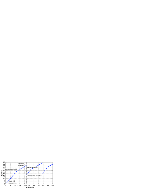
Figure 4: The simple process diagram of FedSAE-Fassa. Each round clients calculate their workload threshold $\theta$ according to the historical information. In the start stage where the clients’ local epoch less than $\theta$ and clients’ local epoch increases by $\gamma_{1}$ each round. In the arise stage where the number of client’s local epoch is greater than $\theta$ and clients’ local epoch increases by $\gamma_{2}$, where $\gamma_{1}$ $\textgreater$ $\gamma_{2}$. Also, if clients drop out then the local epoch of the next round will be halved.

Client selection with Active Learning. Although the aforementioned workload prediction algorithms can reduce stragglers, the quality of the global model should be considered further as not all clients are active in the training process. Therefore, we combine active learning (AL)[37] with FedSAE to select clients with high training value for the global model to participate in training in order to obtain a high-quality global model. In general, some clients’ local models own large loss, and focusing on optimizing these models will greatly improve the quality of the global model[38]. Hence, AL aims to select clients with larger training loss to participate in training. In our framework, the server firstly converts the cross-entropy loss of each client into the corresponding training value to measure the importance of the client. And then, the server converts the training value into selected probability and selects participants for each round according to the probabilities. The training value of client $k$ at round $t$ is calculated as the following equation:

$$\begin{split}v_{k}^{t+1}=\left\{\begin{array}[]{ll}\sqrt{n_{k}}\bar{l}_{k}^{t},&if~{}client~{}k~{}is~{}selected\\ v_{k}^{t},&otherwise\end{array}\right.\end{split}$$ (6)

where $n_{k}$ is the number of samples on client $k$, $\bar{l}_{k}^{t}$ is the average loss of client $k$ at round $t$. At each round, only the loss of participants is refreshed. Each participant computes the evaluation of value $v_{k}^{t}$ and returns it to the server. Then the server turns $v_{k}^{t}$ into a selected probability $p_{k}^{t}$ by the equation as follows:

$$p_{k}^{t}=\frac{e^{\beta*v_{k}^{t}}}{\sum_{k}^{K}e^{\beta*v_{k}^{t}}}$$ (7)

where $\beta$ is the hyper parameter to scale $v_{k}$ to prevent $e^{\beta*v_{k}}$ from being too large of too small to reflect the numerical relationship between the raw data $v_{k}$. Then the server picks participants out according to the selected probabilities $\{p_{1},p_{2},...,p_{n}\}$.

In terms of the cost of FedSAE, compared to FedAvg, the server requires $\mathcal{O}(n)$ extra time to calculate the affordable workload and selected probability. Besides, each client requires $\mathcal{O}(1)$ extra space to store the local loss and $\mathcal{O}(1)$ extra space to store the workload information of its latest model. However, the above-mentioned additional calculation overhead and storage overhead are small enough and can be ignored, which means our algorithm is practical. To verify the rationality of our framework, we will introduce multiple experiments we conducted in the next section.

IV evaluation

In this section, we present the experimental details and results for our framework FedSAE. In subsection IV-B, we show the performance improvement of FedSAE in heterogeneous systems. In subsection IV-C, we sufficiently exhibit the effects of FedSAE combined with AL on convergence.

IV-A Experimental Details

TABLE I: Statistics of FEMNIST, MNIST, Synthetic(1,1) and Sent140.

Dataset	Model	Devices	Samples
MNIST	MCLR	1,000	69,035
FEMNIST		200	18,345
Synthetic(1,1)		100	75,349
Sent140	LSTM	772	40,783

Datasets $\&$ Models. Our evaluation includes two model families on four datasets which are consisted of both image classification tasks and text sentiment analysis tasks. Federated Extended MNIST (FEMNIST)[32] is a 26-class image classification dataset composed of handwritten digits and characters which partition the 62-class data in EMNIST[31] according to writers. The data of FEMNIST is distributed into 200 devices where each device holds only 5 classes as heterogeneous settings. We use multinomial logistic regression (MCLR) with 7850 parameters to train a convex model on FEMNIST. MNIST[30] is a 10-class image classification dataset composed of handwriting digits 0-9. On MNIST, 18,345 samples are divided into 1,000 devices. To simulate obvious heterogeneity, each device holds only 2-class digits and the samples of devices follow a power law. We optimize the model on MNIST with the same training model MCLR as FEMNIST. Sentiment140 (Sent140)[39] is a text sentiment analysis dataset composed of many tweets where each tweet can be extracted as a positive or negative sentiment. The number of clients on Sent140 is 772. We use LSTM to train the model on Sent140. Synthetic[40] is a synthetic federated dataset that consists of 100 devices. We generated Synthetic dataset with the hyperparameter $\alpha=1$, $\beta=1$ (e.g. Synthetic(1,1)) and the data size on clients follows a power law. We use the MCLR classifier to train the model on Synthetic(1,1). The statistics of the above four datasets are shown in TABLE I.

Federated Parameters. All of the above models support training with at least one iteration. We split an epoch into multiple iterations. For example, if a client is required to train 3.5 epochs, then this client will train 3 epochs and $0.5\tau$ iterations where $\tau=\frac{S_{k}}{B}$ varies with the practical iterations of an epoch, $S_{k}$ is the number of samples for client $k$, $B$ is the local mini-batch. In our experiments, we simulate systems heterogeneity by generating the affordable local workloads $E$ of clients at each round with Gaussian Distributions $E\sim\mathcal{N}(\mu,\sigma^{2})$ where $\mu$ $\in$ $[5,10)$, $\sigma\in[\frac{\mu}{4},\frac{\mu}{2})$, $\mu$, $\sigma$ are valued from their regions uniformly. We use the same federated learning settings as introduced in III-A: the number of selected clients per round $K=30$ for MNIST, $K=10$ for FEMNIST, Sent140 and Synthetic(1,1), the mini-batch for local SGD is $B=10$, the learning rate $\eta$ for FEMNIST, MNIST, Sent140, Synthetic(1,1) respectively are 0.03, 0.03, 0.3, 0.01. Specific to FedSAE, we initialize $(L_{k}^{0},H_{k}^{0})$ to (1,2) and we set the inverse ratio parameter $\mathcal{U}=10$, smooth index $\alpha=0.95$, the increment $\gamma_{1}=3$, $\gamma_{2}=1$, scale parameter of AL $\beta=0.01$. For the convenience of understanding, we will reiterate the meaning and value of above FedSAE parameters again when we use it.

Figure 5: Effects of choosing different inverse ratio parameter $\mathcal{U}$. We show the experimental testing accuracy of global model on FEMNIST and MNIST datasets when $\mathcal{U}=1,2,3,10$. Empirically, we find that when $\mathcal{U}=10$, FedSAE-Ira works well.

Baseline $\&$ Metrics. The baseline of this paper is the vanilla FL framework FedAvg[2]. In our experiments, the affordable workload of each client changes over time. We fix the random seed to ensure that the same client has the same affordable workload set on different datasets. If the assignment of clients is less than its affordable workload, then the client can complete the training task, otherwise, it will drop out. For FedAvg, the server fixes the assigned workload $E$ of clients to 15. For FedSAE, the workload of clients is predicted by the server. In order to eliminate the influence of client selection, we fixed the random seed of each round to ensure that when the training framework is different, the server will select the same clients in the same round of the same dataset. Each round we evaluate the global model. To compare each framework intuitively, we draw the top-1 testing accuracy, training loss of global model and drop out rate of clients in the following sections.

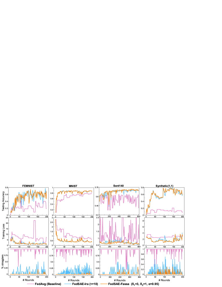
Figure 6: Testing accuracy, training loss, drop out rate of FedSAE-Ira, FedSAE-Fassa relative to FedAvg on four datasets. We simulate a heterogeneous system by giving devices different parameters $\mu$, $\sigma$ of affordable workloads distribution function $\mathcal{N}(\mu,\sigma^{2})$. FedSAE-Ira and FedSAE-Fassa can predict the affordable workloads of devices while FedAvg can not. (1) FedAvg vs. FedSAE-Ira. FedSAE-Ira can increase testing accuracy up to 58% and mitigate straggling up to 88.3%. (2) FedAvg vs. FedSAE-Fassa. Similar to FedSAE-Ira, FedSAE-Fassa brings testing accuracy improvement up to 57.5% and mitigate straggling up to 96.3%. (3) FedSAE-Ira vs. FedSAE-Fassa. FedSAE-Ira improves accuracy +0.4% higher than FedSAE-Fassa while FedSAE-Fassa mitigates stragglers +6.875% than FedSAE-Ira. FedSAE improves absolute testing accuracy by 26.7%. We also report accuracy improvement in TABLE II.

TABLE II: Results of FedSAE-Ira, FedSAE-Fassa on FEMNIST, MNIST, Sent140 and Synthetic(1,1). We show the top-1 testing accuracy and the average drop out rate( see the row of % stragglers in the TABLE) as below. Besides, the percentages of accuracy improvement and stragglers mitigation are calculated.

Dasaset	FedAvg (Baseline)		FedSAE-Ira (Ours)		FedSAE-Fassa (Ours)
	accuracy	% stragglers	accuracy	% stragglers	accuracy	% stragglers
FEMNIST	41.7	97.5	77.8 ($\uparrow$ 36.1)	10.2 ($\downarrow$ 87.3)	75.1 ($\uparrow$ 33.4)	8.0 ($\downarrow$ 89.5)
MNIST	81.9	96.6	89.4 ($\uparrow$ 7.5)	8.3 ($\downarrow$ 88.3)	89.4 ($\uparrow$ 7.5)	0.3 ($\downarrow$ 96.3)
Sent140	63.9	96.5	72.1 ($\uparrow$ 8.2)	10.3 ($\downarrow$ 86.2)	72.4 ($\uparrow$ 8.5)	1.4 ($\downarrow$ 95.1)
Synthetic(1,1)	20.9	97.1	78.9 ($\uparrow$ 58)	11.2 ($\downarrow$ 85.9)	78.4 ($\uparrow$ 57.5)	2.6 ($\downarrow$ 94.5)

IV-B Effects of Affordable Workload Prediction

We divide the experiment of FedSAE into three groups: FedAvg vs. FedSAE-Ira, FedAvg vs. FedSAE-Fassa, FedSAE-Ira vs. FedSAE-Fassa. The former two groups are to illustrate the effects of FedSAE, and the latter group is to illustrate the performance difference between the two prediction algorithms. The details are following:

Figure 7: Effects of assigning different values to $\gamma_{1}$, $\gamma_{2}$ and $\alpha$ in FedSAE-Fassa. We see that when $\gamma_{1}=3$, $\gamma_{2}=1$, $\alpha=0.95$, FedSAE-Fassa works well on both FEMNIST and MNIST.

FedAvg vs. FedSAE-Ira. FedSAE-Ira predicts clients’ local epoch according to the history of completing tasks of the latest round. In FedSAE-Ira, we predict the affordable workload with the increment which is inversely proportional to the amount of the client’s current work. We conduct several experiments on FEMNIST and MNIST to get a suitable value of the inverse ratio parameter $\mathcal{U}$, and some details are shown in Fig. 5. Empirically, we set $\mathcal{U}$ to 10 so the increment is $\frac{10}{E_{k}^{t}}$ if the client performs its assigned workloads successfully. To eliminate the influence of client selection, the server selects clients randomly on both FedSAE-Ira and FedAvg. We implement FedSAE-Ira (Algorithm 2) in Tensorflow[41] and report the performance of FedSAE-Ira and FedAvg in Fig. 6 and TABLE II. We can see that on the four datasets, systems heterogeneity leads to more than $90\%$ of stragglers (see the pink solid lint in the bottom row of Fig. 6). Moreover, from the training loss in the second row of Fig. 6, we can see that FedAvg has a divergent trend on FEMNIST, Sent140 and Synthetic(1,1). The evidence is that the training loss does not decrease but increases. In such a situation, FedSAE-Ira effectively improves the testing accuracy by up to $58\%$ (see the line of Synthetic(1,1) in TABLE II), and reduces the stragglers by up to $88.3\%$. Besides, the convergence rate of the global model is restored. Because FedSAE-Ira predicts an appropriate workload for each client, thus a large number of clients avoid dropping out.

FedAvg vs. FedSAE-Fassa. FedSAE-Fassa predicts clients’ local epoch according to the training history of all of the past communication rounds. We show the experimental results of choosing the suitable parameters (i.e. $\alpha$, $\gamma_{1}$, $\gamma_{2}$) for FedSAE-Fassa in Fig. 7. Empirically, we set smooth index $\alpha$ to 0.95. And we set the increment parameters $\gamma_{1}$, $\gamma_{2}$ to $3$, $1$. The participants of each round also are selected randomly. The experimental results are shown in Fig. 6. Similar to FedSAE-Ira, FedSAE-Fassa brings the accuracy improvement and mitigates straggling. Specifically, FedSAE-Fassa improves the testing accuracy by up to $57.5\%$, which is similar to FedSAE-Ira. Besides, FedSAE-Fassa also reduces stragglers up to $96.3\%$, which is $8\%$ higher than FedSAE-Ira. The reason may be that FedSAE-Fassa makes full use of clients’ past training history of completing tasks, which can more accurately predict the changing characteristics of the affordable workload.

FedSAE-Ira vs. FedSAE-Fassa. In Fig. 6, FedSAE-Ira and FedSAE-Fassa are efficient in accuracy improving and straggler decreasing. To be exact, FedSAE-Ira brings accuracy improvement +0.4% higher than FedSAE-Fassa on average. While FedSAE-Fassa mitigates straggling +6.875% more significantly than FedSAE-Ira on average. From the data in TABLE II, we see that our framework FedSAE improves absolute testing accuracy by 26.7% and reduces the straggle rate by 90.3% on average.

Although accuracy is improved, the convergence rate is still changeless. So we import Active Learning to accelerate the model convergence rate as described in the following section.

Figure 8: Testing accuracy and training loss on FedSAE-Ira with the different training rounds using AL. FedSAE-Ira+AL200 also named full FedSAE-Ira+AL owns the fastest convergence rate.

TABLE III: The number of training rounds for FEMNIST to achieve the goal testing accuracy 60% and MNIST to achieve the goal testing accuracy 84%.

Dataset	# Rounds of using AL in FedSAE-Ira						FedAvg, E=15
	0	20	50	100	150	200
FEMNIST	48	30	31	37	32	32	-
MNIST	25	19	21	19	19	19	-

IV-C Effects of AL

To improve the quality of the global model further, we utilize Active Learning (AL)[37] to dynamically select participants with high training value for the global model. Empirically, we set the scale parameter $\beta$ to $0.01$ which is the same as [38]. As shown in Fig. 8, we conduct multiple experiments with the number of rounds to perform AL as a variable, where the label FedSAE-Ira+ALn represents the client selection strategy is used in the first n training rounds. Particularly, FedSAE-Ira+AL0 represents the pure FedSAE-Ira. Similarly, FedSAE-Ira+AL200 represents full FedSAE-Ira+AL. The experimental results are shown in Fig. 8 which demonstrates that AL improves the convergence speed of the global model. In order to quantify the impact of AL on convergence, we show the number of training rounds for FEMNIST to achieve the goal accuracy 60% and for MNIST to achieve the goal accuracy 84% in TABLE III. From TABLE III, we can see that in the early of the training, compared to pure FedSAE-Ira and FedAvg, FedSAE-Ira+AL can increase the convergence speed of the model by at least 23.5 % on average. However, AL improves the convergence speed while slightly reducing the testing accuracy of the global model i.e. accuracy of FEMNIST and MNIST decreases by up to 2.3%, 0.7% separately. To achieve a compromise between convergence rate and global model accuracy, we recommend using the client selection strategy for the first quarter of the training round.

V conclusion

In this paper, we propose FedSAE, aiming to solve the straggle problems and performance reduction caused by systems heterogeneity. FedSAE allows clients to self-adaptively perform their affordable workloads according to the training history of clients which relies on the two self-adaptive algorithms FedSAE-Ira and FedSAE-Fassa. We explain the design details of these two algorithms and parameters choosing to get efficient performance. Also, we show a series of experimental results on federated datasets to demonstrate that the significant accuracy improvement and stragglers decreasing of our framework in heterogeneous federated learning systems. Our framework, FedSAE, generally improves 26.7% absolute testing accuracy and reduces 90.3% drop out rate on average. Besides, FedSAE can speed up convergence rate of global model. Our future work includes providing convergence analysis for our framework and providing more reliable accuracy improvements for imbalanced datasets when we accelerate model convergence.

References

- [1] J. Konečnỳ, H. B. McMahan, F. X. Yu, P. Richtárik, A. T. Suresh, and D. Bacon, “Federated learning: Strategies for improving communication efficiency,” arXiv preprint arXiv:1610.05492, 2016.
- [2] B. McMahan, E. Moore, D. Ramage, S. Hampson, and B. A. y Arcas, “Communication-efficient learning of deep networks from decentralized data,” in Artificial Intelligence and Statistics. PMLR, 2017, pp. 1273–1282.
- [3] V. Smith, C.-K. Chiang, M. Sanjabi, and A. S. Talwalkar, “Federated multi-task learning,” in Advances in Neural Information Processing Systems, 2017, pp. 4424–4434.
- [4] Q. Yang, Y. Liu, T. Chen, and Y. Tong, “Federated machine learning: Concept and applications,” ACM Transactions on Intelligent Systems and Technology (TIST), vol. 10, no. 2, pp. 1–19, 2019.
- [5] A. Hard, K. Rao, R. Mathews, S. Ramaswamy, F. Beaufays, S. Augenstein, H. Eichner, C. Kiddon, and D. Ramage, “Federated learning for mobile keyboard prediction,” arXiv preprint arXiv:1811.03604, 2018.
- [6] L. Yang, B. Tan, V. W. Zheng, K. Chen, and Q. Yang, “Federated recommendation systems,” in Federated Learning. Springer, 2020, pp. 225–239.
- [7] T. S. Brisimi, R. Chen, T. Mela, A. Olshevsky, I. C. Paschalidis, and W. Shi, “Federated learning of predictive models from federated electronic health records,” International journal of medical informatics, vol. 112, pp. 59–67, 2018.
- [8] T. Li, A. K. Sahu, A. Talwalkar, and V. Smith, “Federated learning: Challenges, methods, and future directions,” IEEE Signal Processing Magazine, vol. 37, no. 3, pp. 50–60, 2020.
- [9] K. Bonawitz, H. Eichner, W. Grieskamp, D. Huba, A. Ingerman, V. Ivanov, C. Kiddon, J. Konečnỳ, S. Mazzocchi, H. B. McMahan et al., “Towards federated learning at scale: System design,” arXiv preprint arXiv:1902.01046, 2019.
- [10] T. Li, A. K. Sahu, M. Zaheer, M. Sanjabi, A. Talwalkar, and V. Smith, “Federated optimization in heterogeneous networks,” arXiv preprint arXiv:1812.06127, 2018.
- [11] T. Nishio and R. Yonetani, “Client selection for federated learning with heterogeneous resources in mobile edge,” in ICC 2019-2019 IEEE International Conference on Communications (ICC). IEEE, 2019, pp. 1–7.
- [12] Y. Zhao, M. Li, L. Lai, N. Suda, D. Civin, and V. Chandra, “Federated learning with non-iid data,” arXiv preprint arXiv:1806.00582, 2018.
- [13] L. Huang, Y. Yin, Z. Fu, S. Zhang, H. Deng, and D. Liu, “Loadaboost: Loss-based adaboost federated machine learning on medical data,” arXiv preprint arXiv:1811.12629, 2018.
- [14] M. Duan, D. Liu, X. Chen, Y. Tan, J. Ren, L. Qiao, and L. Liang, “Astraea: Self-balancing federated learning for improving classification accuracy of mobile deep learning applications,” in 2019 IEEE 37th International Conference on Computer Design (ICCD). IEEE, 2019, pp. 246–254.
- [15] T. Li, A. K. Sahu, M. Zaheer, M. Sanjabi, A. Talwalkar, and V. Smithy, “Feddane: A federated newton-type method,” in 2019 53rd Asilomar Conference on Signals, Systems, and Computers. IEEE, 2019, pp. 1227–1231.
- [16] X. Yao, T. Huang, C. Wu, R. Zhang, and L. Sun, “Towards faster and better federated learning: A feature fusion approach,” in 2019 IEEE International Conference on Image Processing (ICIP). IEEE, 2019, pp. 175–179.
- [17] H. Yu, S. Yang, and S. Zhu, “Parallel restarted sgd with faster convergence and less communication: Demystifying why model averaging works for deep learning,” in Proceedings of the AAAI Conference on Artificial Intelligence, vol. 33, 2019, pp. 5693–5700.
- [18] X. Li, K. Huang, W. Yang, S. Wang, and Z. Zhang, “On the convergence of fedavg on non-iid data,” arXiv preprint arXiv:1907.02189, 2019.
- [19] K. Bonawitz, V. Ivanov, B. Kreuter, A. Marcedone, H. B. McMahan, S. Patel, D. Ramage, A. Segal, and K. Seth, “Practical secure aggregation for privacy-preserving machine learning,” in Proceedings of the 2017 ACM SIGSAC Conference on Computer and Communications Security, 2017, pp. 1175–1191.
- [20] H. Tang, S. Gan, C. Zhang, T. Zhang, and J. Liu, “Communication compression for decentralized training,” Advances in Neural Information Processing Systems, vol. 31, pp. 7652–7662, 2018.
- [21] S. Samarakoon, M. Bennis, W. Saad, and M. Debbah, “Federated learning for ultra-reliable low-latency v2v communications,” in 2018 IEEE Global Communications Conference (GLOBECOM). IEEE, 2018, pp. 1–7.
- [22] S. Caldas, J. Konečny, H. B. McMahan, and A. Talwalkar, “Expanding the reach of federated learning by reducing client resource requirements,” arXiv preprint arXiv:1812.07210, 2018.
- [23] E. Jeong, S. Oh, H. Kim, J. Park, M. Bennis, and S.-L. Kim, “Communication-efficient on-device machine learning: Federated distillation and augmentation under non-iid private data,” arXiv preprint arXiv:1811.11479, 2018.
- [24] H. B. McMahan, D. Ramage, K. Talwar, and L. Zhang, “Learning differentially private recurrent language models,” arXiv preprint arXiv:1710.06963, 2017.
- [25] M. Mohri, G. Sivek, and A. T. Suresh, “Agnostic federated learning,” in 36th International Conference on Machine Learning, ICML 2019. International Machine Learning Society (IMLS), 2019, pp. 8114–8124.
- [26] T. Li, M. Sanjabi, A. Beirami, and V. Smith, “Fair resource allocation in federated learning,” in International Conference on Learning Representations, 2019.
- [27] S. A. Rahman, H. Tout, A. Mourad, and C. Talhi, “Fedmccs: Multi criteria client selection model for optimal iot federated learning,” IEEE Internet of Things Journal, 2020.
- [28] N. Ferdinand, H. Al-Lawati, S. C. Draper, and M. Nokleby, “Anytime minibatch: Exploiting stragglers in online distributed optimization,” arXiv preprint arXiv:2006.05752, 2020.
- [29] A. Reisizadeh, H. Taheri, A. Mokhtari, H. Hassani, and R. Pedarsani, “Robust and communication-efficient collaborative learning,” in Advances in Neural Information Processing Systems, 2019, pp. 8388–8399.
- [30] Y. LeCun, L. Bottou, Y. Bengio, and P. Haffner, “Gradient-based learning applied to document recognition,” Proceedings of the IEEE, vol. 86, no. 11, pp. 2278–2324, 1998.
- [31] G. Cohen, S. Afshar, J. Tapson, and A. Van Schaik, “Emnist: Extending mnist to handwritten letters,” in 2017 International Joint Conference on Neural Networks (IJCNN). IEEE, 2017, pp. 2921–2926.
- [32] S. Caldas, P. Wu, T. Li, J. Konečnỳ, H. B. McMahan, V. Smith, and A. Talwalkar, “Leaf: A benchmark for federated settings,” arXiv preprint arXiv:1812.01097, 2018.
- [33] D.-M. Chiu and R. Jain, “Analysis of the increase and decrease algorithms for congestion avoidance in computer networks,” Computer Networks and ISDN systems, vol. 17, no. 1, pp. 1–14, 1989.
- [34] J. He, H.-H. Chen, T. M. Chen, and W. Cheng, “Adaptive congestion control for dsrc vehicle networks,” IEEE communications letters, vol. 14, no. 2, pp. 127–129, 2010.
- [35] M. Allman, V. Paxson, W. Stevens et al., “Tcp congestion control,” 1999.
- [36] D. Haynes, S. Corns, and G. K. Venayagamoorthy, “An exponential moving average algorithm,” in 2012 IEEE Congress on Evolutionary Computation. IEEE, 2012, pp. 1–8.
- [37] B. Settles, “Active learning literature survey,” 2009.
- [38] J. Goetz, K. Malik, D. Bui, S. Moon, H. Liu, and A. Kumar, “Active federated learning,” arXiv preprint arXiv:1909.12641, 2019.
- [39] A. Go, R. Bhayani, and L. Huang, “Twitter sentiment classification using distant supervision,” CS224N project report, Stanford, vol. 1, no. 12, p. 2009, 2009.
- [40] O. Shamir, N. Srebro, and T. Zhang, “Communication-efficient distributed optimization using an approximate newton-type method,” in International conference on machine learning, 2014, pp. 1000–1008.
- [41] M. Abadi, P. Barham, J. Chen, Z. Chen, A. Davis, J. Dean, M. Devin, S. Ghemawat, G. Irving, M. Isard et al., “Tensorflow: A system for large-scale machine learning,” in 12th USENIX symposium on operating systems design and implementation (OSDI), 2016, pp. 265–283.