Generalized-Hukuhara Subgradient and its Application in Optimization Problem with Interval-valued Functions
Abstract
In this article, the concepts of -subgradients and -subdifferentials of interval-valued functions are illustrated. Several important characteristics of the -subdifferential of a convex interval-valued function, e.g., closeness, boundedness, chain rule, etc. are studied. Alongside, we prove that -subdifferential of a -differentiable convex interval-valued function only contains -gradient of that interval-valued function. It is observed that the -directional derivative of a convex interval-valued function in each direction is maximum of all the products of -subgradients and the direction. Importantly, we show that a convex interval-valued function is -Lipschitz continuous if it has -subgradients at each point in its domain. Furthermore, the relations between efficient solutions of an optimization problem with interval-valued function and its -subgradients are derived.
keywords:
(R) Convex programming, -subgradient , -subdifferential , Interval optimization problemsAMS Mathematics Subject Classification (2010): 26B25 90C25 90C30.
1 Introduction
In the real-life decision-making process, we often face the optimization problem with nonsmooth functions and in order to deal with the optimization problems with nonsmooth functions, the concepts of subgradient and subdifferential inevitably arise. Due to inexact and imprecise natures of many real-world occurrences the study of Interval-Valued Functions (IVFs) and Optimization problems with IVFs, known as Interval Optimization Problems (IOP)s, become substantial topics to the researchers. In this article, we illustrate the concepts of subgradient and subdifferential for IVFs, and study the several important characteristics of subgradient and subdifferential of IVFs. We also study the optimality conditions for nonsmooth IOPs. As intervals are the inextricable things in IVFs and IOPs, before making a survey on IVFs and IOPs, we make a survey on the arithmetic and ordering of intervals.
1.1 Literature Survey
In the literature of IVFs, to deal with compact intervals and IVFs, Moore [27] developed interval arithmetic. There are a few limitations (see [16] for details) of Moore’s interval arithmetic; especially, Moore’s interval arithmetic cannot provide the additive inverse of a nondegenerate interval. By a nondegenerate interval, we mean an interval whose upper and lower limits are different. To overcome this difficulty, Hukuhara [19] proposed a new rule for the difference of intervals, known as Hukuhara difference of intervals. Although the Hukuhara difference provides the additive inverse of any compact interval, it is not applicable between all pairs of compact intervals (see [16] for details). For this reason, the ‘nonstandard subtraction’, introduced by Markov [26], has been used and named as generalized Hukuhara difference (-difference) by Stefanini [29]. The generalized Hukuhara difference is applicable for all pairs of compact intervals and it also provides the additive inverse of any compact interval.
Unlike the real numbers, intervals are not linearly ordered. Isibuchi and Tanaka [20] suggested a few partial ordering relations of intervals. In [5] some ordering relations based on the parametric representation of intervals are proposed. Also, an ordering relation of intervals is provided in [11] by a bijective map from the set of intervals to . However, all the ordering relations of [5, 11] can be derived from the ordering relations of [20]. The concept of variable ordering relation of intervals is introduced in [17].
Calculus is one of the most important tools in functional analysis. Therefore, as like the real-valued, vector-valued functions, the development of the calculus for IVFs is much more essential to study the characteristics of IVFs. In order to develop the calculus of IVFs, the concept of differentiability of IVFs was initially introduced by Hukuhara [19] with the help of Hukuhara difference of intervals. However, this definition of Hukuhara differentiability is restrictive [10]. Based on -difference, the concepts of -derivative, -partial derivative, -gradient, and -differentiability for IVFs are provided in [9, 12, 26, 30, 31]. Lupulescu studied the differentiability and the integrability for the IVFs on time scales in [23] and developed the fractional calculus for IVFs in [24]. The concept of directional -derivative for IVF is depicted in [3, 31]. Recently, Ghosh et al. [16] have introduced the idea of -Gâteaux derivative, and -Fréchet derivative of IVFs.
Based on the existing ordering relations of intervals and calculus of IVFs many authors developed the theories to characterize the solutions to IOPs. For instance, using the concept of Hukuhara differentiability, Wu proposed Karush-Kuhn-Tucker (KKT) conditions for IOPs in [34]. In [35], Wu presented the solution concepts of IOPs with the help of bi-objective optimization. Also, Wu presented some duality conditions for IOPs in [36, 37]. Using the concept of -differentiability, Chalco-Cano et al. [9] presented KKT conditions for IOPs. Ghosh et al. [15] developed generalized KKT conditions to obtain the solution of the IOPs. Recently, Stefanini et al. [31] have depicted the optimality conditions for IOPs using the concepts of directional -derivative and total -derivative of IVFs, and Ghosh et al. have developed the optimality conditions for IOPs using the concepts of -Gâteaux derivative, and -Fréchet derivative of IVFs.
The authors of [1, 2, 22, 32, 33] proposed various optimality and duality conditions for nonsmooth IOPs converting them into real-valued multiobjective optimization. However, in this approach, one needs the closed-form of boundary functions of the interval-valued objective and constrained functions as readily available, which is practically difficult. Because even for a very simple IVF F, the closed forms of the lower boundary function and upper boundary function are not easy to execute; for instance, consider for all . Apart from these, based on parametric representations of the IVFs, some authors [5, 12, 14] studied IOPs and developed theories to obtain the solutions to IOPs by converting them into real-valued optimization problems. The authors of [6] proposed some optimality conditions and duality results of a nonsmooth convex IOP using the parametric representation of its interval-valued objective and constrained functions. However, the parametric process is also practically difficult. Because in the parametric process, the number of variables increases with the number of intervals involved in the IVFs, and to verify any property of an IVF one has to verify it for an infinite number of its corresponding real-valued function. For instance, see Definition in [6].
1.2 Motivation and Contribution
From the literature of IVFs and IOPs, it is observed that the concepts of subgradient and subdifferentials for IVFs are not properly introduced. However, the authors of [18] proposed the concepts of subgradient and subdifferentials for -cell convex fuzzy-valued functions (FVFs) and proved that the subdifferentials of convex FVFs are convex. But they didn’t mention about other important properties of subgradient and subdifferentials of FVFs, such as closeness, boundedness, chain rule, etc. of subdifferentials. As IVFs are the special case of FVFs, in this article, at first adopting the concept of subgradient for convex FVFs of the article [18] we define subgradient of convex IVFs (namely -subgradient). Thereafter, we illustrate the concept of subgradient for convex IVFs in terms of linear IVFs. Subsequently, we define subdifferential of convex IVFs (namely -subdifferential) and study its various properties. We prove that -subdifferentials of convex IVFs are closed, and bounded sets. In order to prove these properties, the norm on the set of -continuous bounded linear IVFs is defined and the idea of sequences with their convergence on the set of -tuple of compact intervals is described. Although the author of [25] provided the concept of subgradients for IVFs in terms of linear functions, our concept is more general (please see Remark 6 of this article for details).
Along with the aforementioned properties of -subdifferentials, several important characteristics of -subgradients are also studied in this article. Interestingly, it is observed that if a convex IVF has -subgradients at each point in its domain, then the IVF is -Lipschitz continuous. It is reported that the -directional derivative of a convex IVF is the maximum of the products of the -subgradients and the concerning direction. The chain rule of a convex IVF and the -subgradient of the sum of finite numbers of convex IVFs are illustrated. Also, some optimality conditions of nonsmooth convex IOP without applying the parametric approach are explored in this article. Most importantly, it is to mention that all the proposed definitions and the results of this article are applicable to general IVFs regardless of whether or not
-
(i)
the IVFs can be expressed parametrically, or
-
(ii)
the explicit form of the lower and upper boundary functions of the IVFs can be found.
1.3 Delineation
The proposed work is organized as follows. The next section deals with some basic terminologies and notions of intervals analysis followed by the convexity and calculus of IVFs. The concepts of -subgradients and -subdifferentials of IVFs with their several important characteristics are illustrated in Section 3. It is shown that the -subdifferential of a convex IVF is closed and bounded. It is observed that a -differentiable convex IVF has only one -subgradient. It is also proved that the -directional derivative of a convex interval-valued function in each direction is maximum of all the products of -subgradients and the direction. Further in Section 3, it is shown that a convex IVF is -Lipschitz continuous if it has -subgradients at each point in its domain. Apart from these, The chain rule of a convex IVF and the -subgradient of the sum of finite numbers of convex IVFs are illustrated. The relations between efficient solutions of an IOP with -subgradients of its objective function are derived in Section 4. Finally, the last section is concerned with a few future directions for this study.
2 Preliminaries and Terminologies
This section is devoted to some basic terminologies and notions on intervals. Convexity and calculus of IVFs are also described here. The ideas and notations that we describe in this section are used throughout the paper.
2.1 Interval Arithmetic, Dominance Relation and Sequence of Intervals
Let be the set of real numbers, be the set of all nonnegative real numbers, and be the set of all compact intervals. We denote the elements of by bold capital letters . We represent an element A of with the help of corresponding small letter in the following way
Similarly, , , and so on. It is to note that any singleton set of can be represented by the interval with . In particular, .
In this article, along with the Moore’s interval addition (), substraction (), multiplication (), and division () [27, 28]:
we use -difference () of intervals because for a nondegenerate interval A. The -difference [26, 29] of the interval B from the interval A is defined by the interval C such that
It is to be noted that for and ,
Remark 1.
It is easy to check that the addition of intervals are commutative and associative, and
The algebraic operations on the product space ( times) are defined as follows.
Definition 2.1.
(Algebraic operations on ). Let and be two elements of . An algebraic operation between and , denoted by , is defined by
where .
The authors of [20] defined the ordering relations of intervals of the following types ‘’, ‘’, and ‘’. In this article, we only use ‘’ ordering relation and simply denote by ‘’. Also, it is to mention that in view of the ordering relation ‘’, we define the dominance relations of intervals as follows.
Definition 2.2.
(Dominance relations on intervals). Let A and B be two intervals in .
-
(i)
B is said to be dominated by A if and , and then we write ;
-
(ii)
B is said to be strictly dominated by A if either and or and , and then we write ;
-
(iii)
if B is not dominated by A, then we write ; if B is not strictly dominated by A, then we write ;
-
(iv)
if and , then we say that none of A and B dominates the other, or A and B are not comparable.
Now we illustrate the concept of sequence in and study its convergence. To do so, we need the concepts of norm on as well as on .
Definition 2.3.
Definition 2.4.
(Norm on ). For an , the function , defined by
is a norm on . To prove that the function satisfies all the properties of a norm please see A.
In the rest of the article, we use the symbols ‘’ and ‘’ to denote the norms on and , respectively, but we simply use the symbol ‘’ to denote the usual Euclidean norm on .
Definition 2.5.
(Sequence in ). A function is called sequence in .
Definition 2.6.
(Bounded sequence in ). A sequence in is said to be bounded from below (above) if there exists an (a ) such that
where for any two elements and in ,
A sequence that is both bounded below and above is called a bounded sequence.
Definition 2.7.
(Convergence in ). A sequence in is said to be convergent if there exists a such that
2.2 Convexity and Calculus of IVFs
A function F from a nonempty subset of to is known as an IVF (interval-valued function). For each argument point , the value of F is presented by
where and are real valued functions on such that for all .
In [34], Wu introduced two types of convexity for IVF, i.e., ‘LU-convexity’ and ‘UC-convexity’. However, in this article, we only use LU-convexity for IVF and we read an LU-convex IVF as simply a convex IVF, which is defined follows.
Definition 2.8.
(Convex IVF [34]). Let be a convex set. An IVF is said to be a convex IVF if for any two vectors and in ,
for all with .
It is notable that in Definition 2.8, we have used the notation ‘’ instead of ‘’. Because the ordering relation ‘’ provided in [34] is same as the ordering relation ‘’.
Lemma 2.1.
(See [34]). F is convex if and only if and are convex.
Definition 2.9.
Lemma 2.2.
An IVF F on a nonempty subset of is -continuous if and only if and are continuous.
Proof.
Please see B. ∎
Theorem 2.1.
If an IVF F on a nonempty open convex subset of is convex, then F is -continuous on .
Proof.
Please see C. ∎
Definition 2.10.
(-Lipschitz continuous IVF [16]). Let . An IVF is said to be -Lipschitz continuous on if there exists such that
The constant is called a Lipschitz constant.
Remark 3.
Definition 2.12.
Definition 2.13.
Definition 2.14.
Definition 2.15.
(Linear IVF [16]). Let be a linear subspace of . The function is said to be linear if
-
(i)
,
-
(ii)
for all , either
or none of and dominates the other.
Remark 4.
(See [16]). The IVF that is defined by
is a linear IVF, where ‘’ denotes successive addition of number of intervals.
We denote the set of all -continuous linear IVF on a linear space as .
Definition 2.16.
(Bounded linear interval-valued operator [16]). Let be a real normed space. A linear IVF is said to be a bounded linear operator if there exists such that
Lemma 2.3.
(See [16]). Let be a real normed. If a linear IVF is -continuous at the zero vector of , then it is a bounded linear operator.
The authors of [31] provided the definition of -differentiability for IVFs using the midpoint-radius representation of an IVF F. However, as our main intention in this article is to illustrate all the things regarding IVF whether its lower boundary function and upper boundary function are readily available or not, we consider the Proposition of [31] as the definition of -differentiability for IVFs, which is as follows.
Definition 2.17.
(-differentiability). Let be a nonempty subset of . An IVF is said to be -differentiable at a point if there exists an IVF , where and , an IVF and a such that
where as .
Theorem 2.2.
Theorem 2.3.
(See [31]). Let an IVF F on a nonempty subset of be -differentiable at . Then, F has directional -derivative at for every direction and
Theorem 2.4.
Let an IVF F on a nonempty open convex subset of be -differentiable at . If the function F is convex on , then
Proof.
Please see D. ∎
3 Subdifferentiability of IVFs
Here we describe the concepts -subgradient and -subdifferential for convex IVFs and study their characteristics. In order to do this, we adopt the concept of subgradient for convex FVFs provided in [18].
Definition 3.1.
(gH-subgradient). Let be a nonempty convex subset of . An element is said to be a -subgradient of a convex IVF at if
| (2) |
Due to Remark 4, we can also define the -subgradient as -continuous linear IVF.
A -continuous linear IVF is said to be -subgradient of F at if
| (3) |
where is the smallest linear subspace of containing .
Definition 3.2.
(gH-subdifferential). The set of all -subgradients of the convex IVF at , where is convex, is called -subdifferential of F at .
Throughout this article, we express an element of either as as an element of satisfying (2) or as an element of satisfying (3).
Remark 5.
In view of Theorem 2.4, it is to be noted that if F is -differentiable at , then .
Example 3.1.
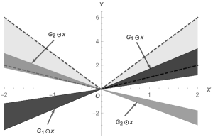
Let be a nonempty convex subset of and an IVF be defined by , where . If is a -subgradient of F at , then according to Definition 3.1, we have
Therefore, for , we have
| (4) |
and for , we have
| (5) |
With the help of (4) and (5), we obtain
Hence, .
Considering , the IVF F is depicted in Figure 1 by the shaded region within dashed lines, and two possible subgradients , of F are illustrated by black and dark gray regions, respectively.
Remark 6.
It is noteworthy that
- (i)
-
(ii)
as IVFs are the special case of FVFs, one may think that we can adopt the concept of subgradient for FVFs of the article [38] as the concept of subgradient for IVFs. However, according to Definition of [38], if we define the -subgradient satisfying the condition
(6) instead of satisfying the condition (2) in Definition 3.1, then Definition 3.1 will be quite restrictive even for a -differentiable IVF. For instance, consider the following example.
Example 3.2.
Now we provide an example of -subdifferential as a collection of -continuous linear IVF through Theorem 3.5. To do so, we introduce the concept of norm on the set of all -continuous linear IVFs on a linear subspace of .
Definition 3.3.
(Norm on ). A norm on the set of all -continuous linear IVF is defined by the function such that
To prove that the function satisfies all the properties of a norm please see E.
Lemma 3.1.
Let be a linear subspace of , and be such that
where C is a closed and bounded interval. Then,
Proof.
Please see F. ∎
Theorem 3.5.
Let be a linear subspace of and be a convex IVF, defined by
where . Then,
Proof.
Let . Therefore, for all nonzero ,
Hence,
∎
Next, we show that a -differentiable convex IVF has only one -subgradient, which is -gradient of the IVF. Also, we show that on a real linear subspace if the -subgradients of a convex IVF at a point exists, then the -directional derivative of the IVF at that point in each direction is maximum of all the products of -subgradients and the direction.
Lemma 3.2.
Let be a nonempty convex subset of and F be a convex IVF on . Then, for an arbitrary
where is -directional derivative of F at in the direction .
Proof.
For an arbitrary , we have
Replacing by , where , we get
which implies
∎
Theorem 3.6.
Let be a nonempty subset of . If an IVF is -differentiable at , then
Proof.
Theorem 3.7.
Let be a convex and -continuous IVF on a real linear subspace of . If -subdifferential of F at an is nonempty, then
where is -directional derivative of F at in the direction .
Proof.
Next, we show that -subdifferentials of a convex IVF are bounded and closed. To do so, we define a mapping by
| (10) |
where , with .
Lemma 3.3.
Proof.
Please see G. ∎
Lemma 3.4.
Proof.
Please see H. ∎
Theorem 3.8.
Let be a compact convex subset of and be a convex IVF. Then, the set is bounded.
Proof.
We claim that the set is bounded. On contrary, there exists a sequence on and an unbounded sequence , where , such that
Let us take , where the mapping is defined by (10). By Definition 3.1 we have
Since F is convex on , in view of Theorem 2.1 and Lemma 2.2, and are continuous on . As and are bounded and the real-valued functions and are continuous, by the property of real-valued function, is finite. Thus, is finite and hence, due to Lemma 3.4, is finite. Therefore, the sequence is bounded, which is a contradiction. Hence, the set is bounded. ∎
Theorem 3.9.
Let be a nonempty convex subset of and F be a convex IVF on . Then, for every , is closed.
Proof.
Let be an arbitrary sequence in which converges to , where and .
Since, , for all we have
i.e.,
| (11) |
Due to Remark 1, without loss of generality, let the first components of be nonnegative and the rest components be negative. Therefore, from (11), we get
Therefore, we get
| (12) |
| (13) |
Since the sequence converges to , in view of Remark 2, the sequences and converge to and , respectively, for all . Thus, by (12) and (13), we have
and
Hence,
for all . Therefore, and hence, is closed. ∎
In the following theorem, we prove that if a convex IVF has -subgradients in all over its domain, then the IVF is -Lipschitz continuous on its domain.
Lemma 3.5.
For any and ,
Proof.
Please see I. ∎
Lemma 3.6.
Let be a nonempty subset of and F be an IVF on such that
where . Then,
Proof.
Please see J. ∎
Theorem 3.10.
Let be a nonempty compact convex subset of and F be a convex IVF on such that F has -subgradient at every . Then, F is -Lipschitz continuous on .
Proof.
Since F has -subgradient at every , there exists a such that
Considering , we have
Hence, F is -Lipschitz continuous on . ∎
Now we show another two important characteristics of -subdifferential of a convex IVF.
Theorem 3.11.
(Chain rule). Let be a nonempty convex subset of and an IVF F be defined by
where is a convex IVF and is an matrix with real entries. Then,
Proof.
By the definition of -subdifferentiability of H at , for any , we have a such that
which implies
Since , by Definition 3.1,
∎
Theorem 3.12.
(-subdifferential of a sum). Let be a nonempty convex subset of and an IVF F be defined by
where each is a convex IVF. Then,
Proof.
We write
where is a matrix, defined by for all and is an IVF, defined by
Thus, by Theorem 3.11, we have
∎
4 Convex IOP and its Optimality Conditions
In this section, we explore the relation of efficient solutions to the following IOP:
| (14) |
where F is a convex IVF on the nonempty convex subset of , with the -subgradients of F. The IOP with convex IVFs is known as convex IOP.
The concept of an efficient solution of the IOP (14) is defined below.
Definition 4.1.
Theorem 4.13.
(Optimality condition). Let be a nonempty convex subset of and be a convex IVF. If for some , where , then is an efficient solution of the IOP (14).
Proof.
For instance, consider the following example.
Example 4.1.
Let us consider the following IOP:
| (15) |
Let , then we have
Thus,
Therefore, .
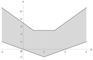
The graph of the IVF F is depicted by the gray shaded region in Figure 2. From Figure 2, it is to be observed that there does not exist any such that . Hence, is the efficient solution of the IOP (15). The following example shows that the converse of Theorem 4.13 is not true.
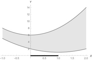
Example 4.2.
Consider the following IOP:
| (16) |
where .
Since and are convex on , the IVF F is convex on by Lemma 2.1. Further, as and are differentiable in , the IVF F is -differentiable in by Remark 3. Hence,
The graph of the IVF F is illustrated by the gray shaded region in Figure 3. From Figure 3, It is clear that for any , there does not exist any such that . Therefore, each is an efficient solution of the IOP (16). The region of the efficient solutions of the IOP (16) is marked by bold black line on the -axis in Figure 3. However, for each ,
and hence, .
Theorem 4.14.
(Optimality condition). Let be a nonempty convex subset of and be a convex IVF. If there exists a for some , such that
| (17) |
then is an efficient solution of the IOP (14).
Proof.
5 Conclusion and Future Directions
In this article, the concepts of -subgradients and -subdifferentials of convex IVFs with their several important characteristics have been provided. It has been shown that the -subdifferential of a convex IVF is closed (Theorem 3.8) and convex (Theorem 3.9); the -subdifferential of a -differentiable convex IVF contains only -gradient of that IVF (Theorem 3.6). It has been observed that on a real linear subspace if the -subgradients of a convex IVF at a point exists, then the -directional derivative of the IVF at that point in each direction is maximum of all the products of -subgradients and the direction (Theorem 3.7). Also, it has been observed that a convex IVF is -Lipschitz continuous if it has -subgradient at each point in its domain (Theorem 3.10). The chain rule of a convex IVF (Theorem 3.11) and the -subgradient of the sum of finite numbers of convex IVFs (Theorem 3.12) have been depicted. Furthermore, the relations between efficient solutions of an IOP with -subgradient of its objective function have been illustrated (Theorem 4.13 and Theorem 4.14).
Although in this article, we have studied various interesting properties of -subgradients and -subdifferentials of convex IVFs but could not make any conclusion about nonemptiness of -subdifferentials. In future, we shall try to make a conclusion about nonemptiness of -subdifferentials. Also, in connection with the proposed research, future research can evolve in several directions as follows.
-
1.
The concept of subdifferential of the dual problem of a constrained convex IOP can be illustrated.
-
2.
A -subgradient technique to obtain the whole solution set of a nonsmooth convex IOP can be derived.
-
3.
The derived results can be applied to solve lasso problem with interval-valued data.
-
4.
The notions of quasidifferentiability for IVFs without the help of its parametric representation can be illustrated.
-
5.
As IVFs are the special case of FVFs and IOPs are the special case of fuzzy optimization problems, similar results can be extended for FVFs and nonsmooth fuzzy optimization problems.
Appendix A Proof of norm on
Proof.
-
(i)
For any element , we have
and
-
(ii)
For any and an element , we obtain
-
(iii)
For any two elements , we have
Without loss of generality, due to Definition 2.3, let
Therefore,
Thus,
Hence, the function is a norm on . ∎
Appendix B Proof of Lemma 2.2
Proof.
Let F be -continuous at a point of the set . Thus, for any such that ,
which implies
Hence, by the definition of -difference we have
i.e., and are continuous at .
Conversely, let the functions and be continuous at . If possible, let F be not -continuous at . Then, as . Therefore, as at least one of the functions and does not tend to . Thus, at least one of the functions and is not continuous at . This contradicts the assumption that the functions and both are continuous at . Hence, F is -continuous at . ∎
Appendix C Proof of Theorem 2.1
Appendix D Proof of Theorem 2.4
Proof.
Let the function F be convex on . Then, for any and , we get
Hence,
which implies
Since F is -differentiable at , taking , by Theorem 2.3, we have
∎
Appendix E Proof of norm on
Proof.
-
(i)
Since and ,
and
Lis the interval-valued zero mapping; by an interval-valued zero mapping we mean an IVF which maps each element of its domain to
-
(ii)
Let and . Then,
-
(iii)
Let . Then,
∎
Appendix F Proof of Lemma 3.1
Appendix G Proof of Lemma 3.3
Proof.
According to Remark 1, without loss of generality, let the first components of be nonnegative and the rest components be negative. Therefore, can be written as
Therefore,
∎
Appendix H Proof of Lemma 3.4
Proof.
Let
be finite. Therefore, all ’s and ’s are finite. Hence,
is finite. ∎
Appendix I Proof of Lemma 3.5
Proof.
Appendix J Proof of Lemma 3.6
References
- [1] Ahmad, I., Singh, D., and Dar, B. A. (2017). Optimality and duality in non-differentiable interval valued multiobjective programming, International Journal of Mathematics in Operational Research, 11(3), 332–356.
- [2] Antczak, T. (2017). Optimality conditions and duality results for nonsmooth vector optimization problems with the multiple interval-valued objective function, Acta Mathematica Scientia, 37B(4), 1133–1150.
- [3] Bao, Y., Zao, B., Bai, E. (2016). Directional differentiability of interval-valued functions, Journal of Mathematics and Computer Science 16(4), 507–515.
- [4] Bertsekas, D. P. (1999). Nonlinear Programming, Athena Scientific, Second Edition.
- [5] Bhurjee, A. K. and Panda, G. (2012). Efficient solution of interval optimization problem, Mathematical Methods of Operations Research, 76, 273–288.
- [6] Bhurjee, A. K. and Padhan, S. K. (2016). Optimality conditions and duality results for non-differentiable interval optimization problems, Journal of Applied Mathematics and Computing, 50(1–2), 59–71.
- [7] Boyd, S. and Vandenberghe, L. (2004). Convex optimization, Cambridge university press.
- [8] Chalco-Cano, Y., Román-Flores, H. and Jiménez-Gamero, M. D. (2011). Generalized derivative and -derivative for set-valued functions, Information Sciences, 181(11), 2177–2188.
- [9] Chalco-Cano, Y., Lodwick, W. A. and Rufian-Lizana, A. (2013). Optimality conditions of type KKT for optimization problem with interval-valued objective function via generalized derivative, Fuzzy Optimization and Decision Making, 12, 305–322.
- [10] Chalco-Cano, Y., Rufian-Lizana, A., Román-Flores H.and Jiménez-Gamero M. D. (2013). Calculus for interval-valued functions using generalized Hukuhara derivative and applications, Fuzzy Sets and Systems, 219, 49–67.
- [11] Costa, T. M., Chalco-Cano, Y., Lodwick, W. A., and Silva, G. N. (2015). Generalized interval vector spaces and interval optimization, Information Sciences, 311, 74–85.
- [12] Ghosh, D. (2017). Newton method to obtain efficient solutions of the optimization problems with interval-valued objective functions, Journal of Applied Mathematics and Computing, 53, 709–731.
- [13] Ghosh, D., Ghosh, D., Bhuiya, S. K. and Patra, L. K. (2018). A saddle point characterization of efficient solutions for interval optimization problems, Journal of Applied Mathematics and Computing, 58(1–2), 193–217.
- [14] Ghosh, D. (2017). A quasi-Newton method with rank-two update to solve interval optimization problems, International Journal of Applied and Computational Mathematics 3(3), 1719–1738.
- [15] Ghosh, D., Singh, A., Shukla, K. K. and Manchanda, K. (2019). Extended Karush-Kuhn-Tucker condition for constrained interval optimization problems and its application in support vector machines, Information Sciences, 504, 276–292.
- [16] Ghosh, D., Chauhan, R. S., Mesiar, R. and Debnath, A. K. (2020). Generalized Hukuhara Gâteaux and Fréchet derivatives of interval-valued functions and their application in optimization with interval-valued functions, Information Sciences, 510, 317-340.
- [17] Ghosh, D., Debnath, A. K. and Pedrycz, W. (2020). A variable and a fixed ordering of intervals and their application in optimization with interval-valued functions, International Journal of Approximate Reasoning, 121, 187–205.
- [18] Hai, S. and Gong, Z. (2018). The differential and subdifferential for fuzzy mappings based on the generalized difference of n-cell fuzzy-numbers, Journal of Computational Analysis and Applications, 24(1), 184–195.
- [19] Hukuhara, M. (1967). Intégration des applications measurables dont la valeur est un compact convexe, Funkcialaj Ekvacioj, 10, 205–223.
- [20] Ishibuchi, H. and Tanaka, H. (1990). Multiobjective programming in optimization of the interval objective function, European Journal of Operational Research, 48(2), 219–225.
- [21] Jahn, J. (2007). Introduction to the theory of nonlinear optimization, Springer Science and Business Media
- [22] Jayswal, A., Ahmad, I., and Banerjee, J. (2016). Nonsmooth interval-valued optimization and saddle-point optimality criteria, Bulletin of the Malaysian Mathematical Sciences Society, 39(4), 1391–1411.
- [23] Lupulescu, V. (2013). Hukuhara differentiability of interval-valued functions and interval differential equations on time scales, Information Sciences, 248, 50–67.
- [24] Lupulescu, V. (2015). Fractional calculus for interval-valued functions, Fuzzy Sets and Systems, 265, 63–85.
- [25] Karaman, E. (2020). Optimality Conditions of Interval-Valued Optimization Problems by Using Subdifferantials Gazi University Journal of Science, 1–7.
- [26] Markov, S. (1979). Calculus for interval functions of a real variable, Computing, 22(4), 325–337.
- [27] Moore, R. E. (1966). Interval Analysis, Prentice-Hall, Englewood Cliffs, New Jersey.
- [28] Moore, R. E. (1987). Method and applications of interval analysis, Society for Industrial and Applied Mathematics.
- [29] Stefanini, L. (2008). A generalization of Hukuhara difference, Soft Methods for Handling Variability and Imprecision, 203–210.
- [30] Stefanini, L. and Bede, B. (2009). Generalized Hukuhara differentiability of interval-valued functions and interval differential equations, Nonlinear Analysis, 71, 1311–1328.
- [31] Stefanini, L. and Arana-Jiménez, M. (2019). Karush-Kuhn-Tucker conditions for interval and fuzzy optimization in several variables under total and directional generalized differentiability, Fuzzy Sets and Systems, 362, 1–34.
- [32] Van Luu, D. and Mai, T. T. (2018). Optimality and duality in constrained interval-valued optimization, 4OR, 16(3), 311–337.
- [33] Van Su, T. and Dinh, D. H. (2020). Duality results for interval-valued pseudoconvex optimization problem with equilibrium constraints with applications, Computational and Applied Mathematics, 39, 1–24.
- [34] Wu, H. C. (2007). The Karush-Kuhn-Tucker optimality conditions in an optimization problem with interval-valued objective function, European Journal of Operational Research, 176, 46–59.
- [35] Wu, H. C. (2008). On interval-valued non-linear programming problems, Journal of Mathematical Analysis and Applications, 338(1), 299–316.
- [36] Wu, H. C. (2008). Wolfe duality for interval-valued optimization, Journal of Optimization Theory and Applications, 138(3), 497–509.
- [37] Wu, H. C. (2010). Duality theory for optimization problems with interval-valued objective functions, Journal of Optimization Theory and Applications, 144(3), 615-628.
- [38] Zhang, C., Yuan, X. H., and Lee, E. S. (2005). Duality theory in fuzzy mathematical programming problems with fuzzy coefficients, Computers and Mathematics with Applications, 49(11-12), 1709–1730.