Cross-Domain Label-Adaptive Stance Detection
Abstract
Stance detection concerns the classification of a writer’s viewpoint towards a target. There are different task variants, e.g., stance of a tweet vs. a full article, or stance with respect to a claim vs. an (implicit) topic. Moreover, task definitions vary, which includes the label inventory, the data collection, and the annotation protocol. All these aspects hinder cross-domain studies, as they require changes to standard domain adaptation approaches. In this paper, we perform an in-depth analysis of 16 stance detection datasets, and we explore the possibility for cross-domain learning from them. Moreover, we propose an end-to-end unsupervised framework for out-of-domain prediction of unseen, user-defined labels. In particular, we combine domain adaptation techniques such as mixture of experts and domain-adversarial training with label embeddings, and we demonstrate sizable performance gains over strong baselines, both (i) in-domain, i.e., for seen targets, and (ii) out-of-domain, i.e., for unseen targets. Finally, we perform an exhaustive analysis of the cross-domain results, and we highlight the important factors influencing the model performance.
1 Introduction
There are many different scenarios in which it is useful to study the attitude expressed in texts, e.g., of politicians with respect to newly proposed legislation (Somasundaran and Wiebe, 2010), of customers regarding new products (Somasundaran and Wiebe, 2009), or of the general public towards public health measures, e.g., aiming to reduce the spread of COVID-19 (Hossain et al., 2020; Glandt et al., 2021). This task, commonly referred to as stance detection, has been studied in many different forms: not just for different domains, but with more substantial differences in the settings, e.g., stance (i) expressed in tweets (Qazvinian et al., 2011; Mohammad et al., 2016; Conforti et al., 2020b) vs. long news articles (Pomerleau and Rao, 2017; Ferreira and Vlachos, 2016) vs. news outlets Stefanov et al. (2020) vs. people Darwish et al. (2020), (ii) with respect to a claim (Chen et al., 2019) vs. a topic, either explicit (Qazvinian et al., 2011; Walker et al., 2012) or implicit (Hasan and Ng, 2013; Gorrell et al., 2019). Moreover, there is substantial variation in (iii) the label inventory, in the exact label definition, in the data collection, in the annotation setup, in the domain, etc. The most crucial of these, which has not been investigated, currently preventing cross-domain studies, is that the label inventories differ between the settings, as shown in Table 1. Labels include not only variants of agree, disagree, and unrelated, but also difficult to cross-map ones, such as discuss and question.
Our goal in this paper is to design a common stance detection framework to facilitate future work on the problem is a cross-domain setting. To this end, we make the following contributions:
-
•
We present the largest holistic study of stance detection to date, covering 16 datasets.
-
•
We propose a novel framework (MoLE) that combines domain-adaptation and label embeddings for learning heterogeneous target labels.
-
•
We further adapt the framework for out-of-domain predictions from a set of unseen targets, based on the label name similarity.
-
•
Our proposed approach outperforms strong baselines both in-domain and out-of-domain.
-
•
We perform an exhaustive analysis of cross-domain results, and find that the source domain, the vocabulary size, and the number of unique target labels are the most important factors for successful knowledge transfer.
Finally, we release our code, models, and data.111The datasets and code are available for research purposes:
https://github.com/checkstep/mole-stance
2 Related Work
Stance Detection
Prior work on stance explored its connection to argument mining (Boltužić and Šnajder, 2014; Sobhani et al., 2015), opinion mining (Wang et al., 2019), and sentiment analysis (Mohammad et al., 2017; Aldayel and Magdy, 2019). Debating platforms were used as data source for stance (Somasundaran and Wiebe, 2010; Hasan and Ng, 2014; Aharoni et al., 2014), and more recently it was Twitter (Mohammad et al., 2016; Gorrell et al., 2019). With time, the definition of stance has become more nuanced (Küçük and Can, 2020), as well as its applications Zubiaga et al. (2018); Hardalov et al. (2021b). Settings vary with respect to implicit (Hasan and Ng, 2013; Gorrell et al., 2019) or explicit topics (Augenstein et al., 2016; Stab et al., 2018; Allaway and McKeown, 2020), claims (Baly et al., 2018; Chen et al., 2019; Hanselowski et al., 2019; Conforti et al., 2020a, b) or headlines (Ferreira and Vlachos, 2016; Habernal et al., 2018; Mohtarami et al., 2018).
The focus, however, has been on homogeneous text, as opposed to cross-platform or cross-domain. Exceptions are Stab et al. (2018), who worked on heterogeneous text, but limited to eight topics, and Schiller et al. (2021), who combined datasets from different domains, but used in-domain multi-task learning, and Mohtarami et al. (2019) and Hardalov et al. (2021a), who used a cross-lingual setup. In contrast, we focus on cross-domain learning on 16 datasets, and out-of-domain evaluation.
Domain Adaptation
Domain adaptation was studied in supervised settings, where in addition to the source-domain data, a (small) amount of labeled data in the target domain is also available (Daumé III, 2007; Finkel and Manning, 2009; Donahue et al., 2013; Yao et al., 2015; Mou et al., 2016; Lin and Lu, 2018), and in unsupervised settings, without labeled target-domain data (Blitzer et al., 2006; Lipton et al., 2018; Shah et al., 2018; Mohtarami et al., 2019; Bjerva et al., 2020; Wright and Augenstein, 2020). Recently, domain adaptation was applied to pre-trained Transformers (Lin et al., 2020). One direction therein are architectural changes (method-centric): Ma et al. (2019) proposed curriculum learning with domain-discriminative data selection, Wright and Augenstein (2020) investigated an unsupervised multi-source approach with Mixture of Experts and domain adversarial training (Ganin et al., 2016).
Label Embeddings
Label embeddings can capture, in an unsupervised fashion, the complex relations between target labels for multiple datasets or tasks. They can boost the end-task performance for various deep learning architectures, e.g., CNNs (Zhang et al., 2018; Pappas and Henderson, 2019), RNNs (Augenstein et al., 2018, 2019), and Transformers (Chang et al., 2020). Recent work has proposed different perspectives for learning label embeddings: Beryozkin et al. (2019) trained a named entity recogniser from heterogeneous tag sets, Chai et al. (2020) used label descriptions for text classification, Rethmeier and Augenstein (2020) explored contrastive label embeddings for long-tail learning.
In our work, we propose an end-to-end framework to learn from heterogeneous labels based on unsupervised domain adaptation and label embeddings, and an unsupervised approach to obtain predictions for an unseen set of user-defined targets, using the similarity between label names.
| Dataset | Target | Context | Labels | Source |
| arc (Hanselowski et al. 2018; Habernal et al. 2018) | Headline | User Post | unrelated (75%), disagree (10%), agree (9%), discuss (6%) | Debates |
| iac1 (Walker et al., 2012) | Topic | Debating Thread | pro (55%), anti (35%), other (10%) | Debates |
| perspectrum (Chen et al., 2019) | Claim | Perspective Sent. | support (52%), undermine (48%) | Debates |
| poldeb (Somasundaran and Wiebe, 2010) | Topic | Debate Post | for (56%), against (44%) | Debates |
| scd (Hasan and Ng, 2013) | None (Topic) | Debate Post | for (60%), against (40%) | Debates |
| emergent (Ferreira and Vlachos, 2016) | Headline | Article | for (48%), observing (37%), against (15%) | News |
| fnc1 (Pomerleau and Rao, 2017) | Headline | Article | unrelated (73%), discuss (18%), agree (7%), disagree (2%) | News |
| snopes (Hanselowski et al., 2019) | Claim | Article | agree (74%), refute (26%) | News |
| mtsd (Sobhani et al., 2017) | Person | Tweet | against (42%), favor (35%), none (23%) | Social Media |
| rumor (Qazvinian et al., 2011) | Topic | Tweet | endorse (35%), deny (32%), unrelated (18%), question (11%), neutral (4%) | Social Media |
| semeval2016t6 (Mohammad et al., 2016) | Topic | Tweet | against (51%), none (24%), favor (25%) | Social Media |
| semeval2019t7 (Gorrell et al., 2019) | None (Topic) | Tweet | comment (72%), support (14%), query (7%), deny (7%) | Social Media |
| wtwt (Conforti et al., 2020b) | Claim | Tweet | comment (41%), unrelated (38%), support (13%), refute (8%) | Social Media |
| argmin (Stab et al., 2018) | Topic | Sentence | argument against (56%), argument for (44%) | Various |
| ibmcs (Bar-Haim et al., 2017) | Topic | Claim | pro (55%), con (45%) | Various |
| vast (Allaway and McKeown, 2020) | Topic | User Post | con (39%), pro (37%), neutral (23%) | Various |
3 Stance Detection Datasets
In this section, we provide a brief overview of the 16 stance datasets included in our study, and we show their key characteristics in Table 1. More details are given in Section 3.1 and in the Appendix (Section B.1). We further motivate the source groupings used in our experiments and analysis (Section 3.3).
3.1 Datasets
arc The Argument Reasoning Comprehension dataset has posts from the New York Times debate section on immigration and international affairs.
argmin The Argument Mining corpus presents arguments relevant to a particular topic from heterogenous texts. Topics include controversial keywords like death penalty and gun control.
emergent The Emergent222http://www.emergent.info/ dataset is a collection of articles from rumour sites annotated by journalists.
fnc1 The Fake News Challenge dataset consists of news articles whose stance towards headlines is provided. It spans 300 topics from Emergent.22footnotemark: 2
iac1 The Internet Argument Corpus V1 consists of Quote–Response pairs from a debating forum on topics related to US politics.
ibmcs This dataset expands the IBM argumentative structure dataset (Aharoni et al., 2014) to 55 topics and provides topic–claim pairs (from IBM Project Debater333IBM Project Debater http://www.research.ibm.com/artificial-intelligence/project-debater/) along with their stance annotations.
mtsd The Multi-Target Stance Detection dataset includes tweets related to the 2016 US Presidential election with a specific focus on multiple targets of interest expressed in each tweet.
perspectrum The Perspectrum dataset provides several perspectives towards a given claim gathered from a number of debating websites.
poldeb The Ideological On-Line Debates corpus provides opinion–target pairs from several debating platforms encapsulating different domains.
rumor The Rumor Has It dataset presents tweets for the task of Belief Classification, where users believe, question, or refute curated rumours.
vast The Varied Stance Topics dataset consists of topic–comment pairs from the The New York Times Room for Debate section. The dataset covers a large variety of topics in order to facilitate zero-shot learning on new unseen topics.
wtwt Will-They-Won’t-They presents a large number of annotated tweets from the financial domain relating to five merger and acquisition operations.
scd The Stance Classification dataset provides debate posts from four domains including Obama and Gay Rights. As highlighted in Table 2, while the posts are gathered from defined domains, they are not part of the training set and need to be inferred.
semeval2016t6 The SemEval-2016 Task 6 dataset provides tweet–target pairs for 5 targets including Atheism, Feminist Movement, and Climate Change.
semeval2019t7 The SemEval-2019 Task 9 dataset aims to model authors’ stance towards a particular rumour. It provides annotated tweets supporting, denying, querying, or commenting on the rumour.
snopes The Snopes dataset provides several controversial claims and their corresponding evidence texts from the US-based fact-checking website Snopes,444http://www.snopes.com annotated for the text in support of, refuting, or having no stance towards a claim.
3.2 Dataset Characteristics
| Dataset | Train | Dev | Test | Total |
| arc | 12,382 | 1,851 | 3,559 | 17,792 |
| argmin | 6,845 | 1,568 | 2,726 | 11,139 |
| emergent | 1,770 | 301 | 524 | 2,595 |
| fnc1 | 42,476 | 7,496 | 25,413 | 75,385 |
| iac1 | 4,227 | 454 | 924 | 5,605 |
| ibmcs | 935 | 104 | 1,355 | 2,394 |
| mtsd* | 3,718 | 520 | 1,092 | 5,330 (8,910) |
| perspectrum | 6,978 | 2,071 | 2,773 | 11,822 |
| poldeb | 4,753 | 1,151 | 1,230 | 7,134 |
| rumor* | 6,093 | 471 | 505 | 7,276 (10,237) |
| scd | 3,251 | 624 | 964 | 4,839 |
| semeval2016t6 | 2,497 | 417 | 1,249 | 4,163 |
| semeval2019t7 | 5,217 | 1,485 | 1,827 | 8,529 |
| snopes | 14,416 | 1,868 | 3,154 | 19,438 |
| vast | 13,477 | 2,062 | 3,006 | 18,545 |
| wtwt | 25,193 | 7,897 | 18,194 | 51,284 |
| Total | 154,228 | 30,547 | 68,495 | 253,270 |
As is readily apparent from Table 1, the datasets differ based on the nature of the target and the context, as well as the stance labels.
The Target is the object of the stance. It can be a Claim, e.g., “Corporal punishment be used in K-12 schools.”, a Headline, e.g., “A meteorite landed in Nicaragua”, a Person, a Topic, e.g., abortion, healthcare, or None (i.e., an implicit target). Respectively, the Context, which is where the stance is expressed, can be an Article, a Claim, a Post, e.g., in a debate, a Thread, i.e., a chain of forum posts, a Sentence, or a Tweet. More examples from each dataset can be found in Table 7 in Appendix B.
Moreover, the diversity of the datasets is also reflected in their label names, ranging from different variants of positive, negative, and neutral to labels such as query or comment. The mapping between them is one of the core challenges we address, and it is discussed in more detail in Section 4.2.
Finally, the datasets differ in their size (see Table 2), varying from 800 to 75K examples. A complementary analysis of their quantitative characteristics, such as how the splits were chosen, the similarity between their training and testing parts, and their vocabularies, can be found in Appendix B.
3.3 Source Groups
Defining source groups/domains is an important part of this study, as they allow for better understanding of the relationship between datasets, which we leverage through domain-adaptive modelling (Section 4). Moreover, we use them to outline phenomena in the results that similar datasets share (Section 5). Table 1 shows these groupings.
Based on the aforementioned definitions of targets and context, we define the following groups: (i) Debates, (ii) News, (iii) Social Media, and (iv) Various.
We combine argmin (Web searches), ibmcs (Encyclopedia), and vast into Various, since they do not fit into any other group.
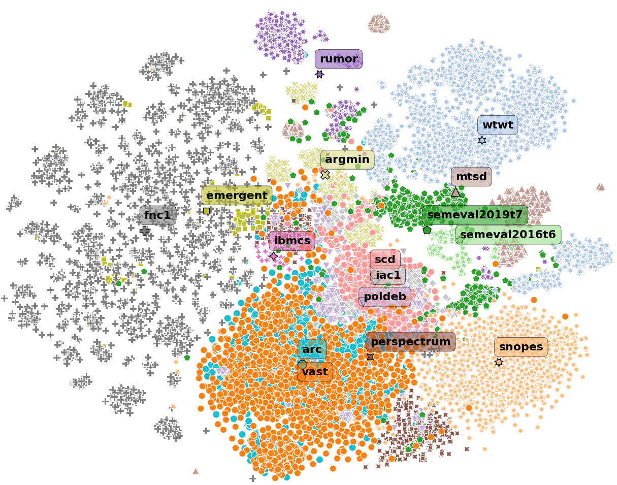
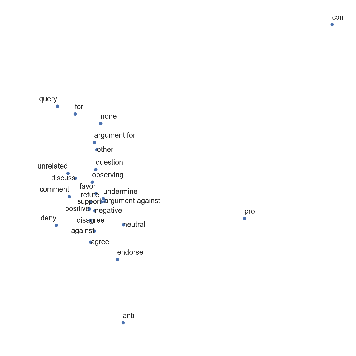
To demonstrate the feasibility of our groupings, we plot the 16 datasets in a latent vector space. We proportionally sample 25K examples, and we pass them through a RoBERTaBase (Liu et al., 2019) cased model without any training. The input has the following form: [CLS] context [SEP] target. Next, we take the [CLS] token representations, and we plot them in Figure 1 using tSNE (van der Maaten and Hinton, 2008). We can see that Social Media datasets are grouped top-right, Debates are in the middle, and News are on the left (except for Snopes). The Various datasets, ibmcs and argmin, are placed in between the aforementioned groups (i.e., Debates and News), and argmin is scattered into small clusters, confirming that they do not fit well into other source categories. Moreover, the figure reflects the strong connections between vast and arc, as well as between fnc1 and emergent, as the former is derived from the latter. Finally, the clusters are well-separated and do not overlap, which highlights the rich diversity of the datasets, each of which has its own definition of stance.
4 Method
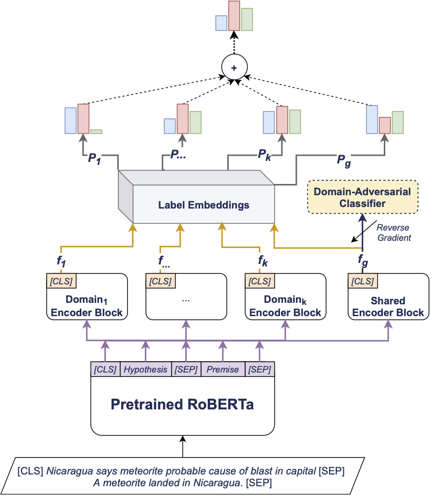
We propose a novel end-to-end framework for cross-domain label-adaptive stance detection. Our architecture (see Figure 2) is based on input representations from a pre-trained language model, adapted to source domains using Mixture-of-Experts and domain adversarial training (Section 4.1). We further use self-adaptive output representations obtained via label embeddings, and unsupervised alignment between seen and unseen target labels for out-of-domain datasets.
Unlike previous work, we focus on learning the relationship between datasets and their label inventories in an unsupervised fashion. Moreover, our Mixture-of-Experts model is more compact than the one proposed by Wright and Augenstein (2020), as we introduce a parameter-efficient architecture with layers that are shared between the experts. Finally, we explore the capability of the model to predict from unseen user-defined target.
With this framework, we solve two main challenges: (i) training domain-adaptive models over a large number of datasets from a variety of source domains, and (ii) predicting an unseen label from a disjoint set of over 50 unique labels.
4.1 Cross-Domain Stance Detection
Mixture-of-Experts (MoE)
is a well-known technique for multi-source domain adaptation (Guo et al., 2018; Li et al., 2018). Recently, this framework was extended to large pre-trained Transformers (Wright and Augenstein, 2020).
In particular, for each domain , there is a domain expert , and a shared, global model . We define , as we use four different domains (see Section 3.3), making this approach appealing to further encourage knowledge sharing between datasets. Further, the models produce a set of probabilities from each expert and from the global model, for all the (often shared) target labels. Then, the final output of the model is obtained by passing these predictions through a combination function, e.g., mean average, weighted average, or attention-based combination (Wright and Augenstein, 2020). We use mean average to gather the final distribution across the label space:
| (1) |
Mixture-of-Experts with Label Embeddings (MoLE)
We propose several changes to Mixture-of-Experts to improve the model’s parameter efficiency, reduce training and inference times, and allow for different label inventories for each task.555In contrast, the model of Wright and Augenstein (2020) requires that the datasets use the same labels. First, in contrast to Wright and Augenstein (2020), we use a shared encoder, here, RoBERTa (Liu et al., 2019), instead of a separate large Transformer model for each domain. Next, for each domain expert and the global shared model, we add a single Transformer (Vaswani et al., 2017) layer on top of the encoder block. We thereby retain the domain experts while sharing information through the encoder. This approach reduces the number of parameters by a factor of the size of the entire model divided by the size of a single layer, i.e., we only use four additional layers (one such encoder block per domain) instead of 48 (the number of layers in RoBERTaBase, not counting embedding layers). For convenience, we set the hidden sizes in the newly-added blocks to match the encoder’s. Next, each domain expert receives as input the representations from the shared encoder of all tokens in the original sequence. Finally, we obtain a domain-specific and a global representation for the input sentence from the [CLS] tokens. These hidden representations are denoted as , where is the number of domains, and is the model’s hidden size. They are passed through a single label embedding layer to obtain the probability distributions.
Domain-Adversarial training
was introduced as part of the Domain-adversarial neural networks (DANN) (Ganin and Lempitsky, 2015). The aim is to learn a task classifier by confusing an auxiliary domain classifier optimised to predict a meta target, i.e., the domain of an example. This approach has shown promising results for many NLP applications (Li et al., 2018; Gui et al., 2017; Wright and Augenstein, 2020). Formally, it forces the model to learn domain-invariant representations, both for the source and for the target domains. The latter is done with an adversarial loss function, where we minimise the task objective , and maximise the confusion in the domain classifier for an input sample (see Eq. 2). We implement this with a gradient reversal layer, which ensures that the source and the target domains are made to be similar.
| (2) |
4.2 Cross-Domain Label-Adaptive Prediction
The second major challenge is how to obtain predictions for out-of-domain datasets. We want to emphasise that just a few of our 16 datasets share the same set of labels (see Section 3); yet, many labels in different datasets are semantically related.
Label Embeddings (LEL)
In multi-task learning, each task typically has its own task-specific labels (in our case, dataset-specific labels), which are predicted in a joint model using separate output layers. However, these dataset-specific labels are not entirely orthogonal to each other (see Section 3). Therefore, we adopt label embeddings to encourage the model to learn task relations in an unsupervised fashion using a common vector space. In particular, we add a Label Embeddings Layer, or LEL, Augenstein et al. (2018)), which learns a label compatibility function between the hidden representation of the input , here the one from the [CLS] token, and an embedding matrix :
| (3) |
where is the shared label embedding matrix for all datasets, and is a hyper-parameter for the dimensionality of each vector.
We set the size of the embeddings to match the hidden size of the model, and obtain the hidden representation from the last layer of the pre-trained language model. Afterwards, we optimise a cross-entropy objective over all labels, masking the unrelated ones and keeping visible only the ones from the target datasets for a sample in the batch. We use the same masking procedure at inference time.
Label-Adaptive Prediction
In an unsupervised out-of-domain setting, there is no direct way to obtain a probability distribution over the set of test labels. Label embeddings are an easy indirect option for obtaining these predictions, as they can be used to measure the similarity between source and target labels. We investigate several alternatives.
Hard Mapping A supervised option is to define a set of meta-groups (hard labels), here six, as shown in Table 3, then to train the model on these labels. E.g., if the out-of-domain dataset is snopes, then its labels are replaced with meta-group labels – agree positive, and refute negative, and thus we can directly use the predictions from the model for out-of-domain datasets. However, this approach has several shortcomings: (i) labels have to be grouped manually, (ii) the meta-groups should be large enough to cover different task definitions, e.g. the dataset’s label inventory may vary in size, and, most importantly, (iii) any change in groupings would require full model re-training.
| Group | Task__Labels Included |
| Positive | arc__agree, argmin__argument for, emergent__for, fnc1__agree, iac1__pro, mtsd__favor, perspectrum__support, poldeb__for, rumor__endorse, scd__for, semeval2016t6__favor, semeval2019t7__support, snopes__agree, vast__pro, wtwt__support |
| Negative | arc__disagree, argmin__argument against, emergent__against, fnc1__disagree, iac1__anti, ibmcs__con, mtsd__against, perspectrum__undermine, poldeb__against, rumor__deny, scd__against, semeval2016t6__against, semeval2019t7__deny, snopes__refute, vast__con, wtwt__refute |
| Discuss | arc__discuss, emergent__observing, fnc1__discuss, rumor__question, semeval2019t7__query, wtwt__comment |
| Other | arc__unrelated, fnc1__unrelated, iac1__other, mtsd__none, rumor__unrelated, semeval2019t7__comment, wtwt__unrelated |
| Neutral | rumor__neutral, vast__neutral |
Soft Mapping To overcome these limitations, we propose a simple, yet effective, entirely unsupervised procedure involving only the label names. More precisely, we measure the similarity between the names of the labels across datasets. This is an intuitive approach for finding a matching label without further context, e.g., for is probably close to agree, and refute is close to against. In particular, given a set of out-of-domain target labels , and a set of predictions from in-domain labels , , we select the label from with the highest cosine similarity to the predicted label :
| (4) |
where is the number of out-of-domain labels, the number of out-of-domain examples, and the number of in-domain labels. The procedure can generalise to any labels, without the need for additional supervision. To illustrate this, the embedding spaces of pre-trained embedding models for our 16 datasets are visualised in Appendix C.
Weak Mapping Nevertheless, as proposed, this procedure only takes label names into account, in contrast to the hard labels that rely on human expertise. This makes combining the labels in a weakly supervised manner an appealing alternative. For this, we measure label similarities as proposed, but incorporate some supervision for defining the embeddings. We first group the labels into six separate categories to define their nearest neighbours (see Table 3). Then, we choose the most similar label for the target domain from these neighbours.
The list of neighbours is defined by the group of the predicted label. However, there is no guarantee that there will be a match for the target domain within the same group, and thus we further define group-level neighbourhoods (see Table 4), as it is not feasible to define the neighbours for all (more than 50) labels individually. One drawback is that each new label/group must define a neighbourhood with similar labels – and vice-versa, it should be assigned a position in the neighbourhoods of the existing labels.
| Group | Closest Neighbours |
| Positive | Other, Neutral, Discuss, Negative |
| Other | Neutral, Discuss, Positive, Negative |
| Neutral | Discuss, Other, Positive, Negative |
| Discuss | Neutral, Other, Negative, Positive |
| Negative | Discuss, Neutral, Other, Positive |
4.3 Training
We train the model using the following loss:
| (5) | |||
| (6) | |||
| (7) |
First, we sum the source-domain loss () with the meta-target loss from the domain expert sub-network (), where the contribution of each is balanced by a single hyper-parameter , set to . Next, we add the domain adversarial loss (), and we multiply it by a weighting factor , which is set to a small positive number to prevent this regulariser from dominating the overall loss. We set to . Furthermore, since our dataset is quite diverse even in the four source domains that we outlined, we optimise the domain-adaptive loss towards a meta-class for each dataset, instead of the domain.
5 Experiments
| F1avg. | arc | iac1 | perspectrum | poldeb | scd | emergent | fnc1 | snopes | mtsd | rumor | semeval16 | semeval19 | wtwt | argmin | ibmcs | vast | |
| Majority class baseline | 27.60 | 21.45 | 21.27 | 34.66 | 39.38 | 35.30 | 21.30 | 20.96 | 43.98 | 19.49 | 25.15 | 24.27 | 22.34 | 15.91 | 33.83 | 34.06 | 17.19 |
| Random baseline | 35.19 | 18.50 | 30.66 | 50.06 | 48.67 | 50.08 | 31.83 | 18.64 | 45.49 | 33.15 | 20.43 | 31.11 | 17.02 | 20.01 | 49.94 | 50.08 | 33.25 |
| Logistic Regression | 41.35 | 21.43 | 28.68 | 61.33 | 72.30 | 44.63 | 61.30 | 24.02 | 59.32 | 44.29 | 19.31 | 48.92 | 22.34 | 32.32 | 51.06 | 37.13 | 33.31 |
| MTL w/ BERTBase | 63.11 | 63.19 | 45.30 | 78.62 | 50.76 | 64.03 | 86.23 | 74.48 | 71.55 | 56.36 | 60.26 | 68.28 | 61.03 | 63.59 | 59.05 | 68.55 | 38.42 |
| MTL w/ RoBERTaBase | 65.12 | 64.52 | 35.73 | 82.38 | 53.83 | 59.43 | 83.91 | 75.29 | 74.95 | 65.87 | 71.23 | 70.46 | 59.42 | 67.64 | 61.79 | 77.27 | 38.21 |
| MoLE (Our Model) | 65.55 | 63.17 | 38.50 | 85.27 | 50.76 | 65.91 | 83.74 | 75.82 | 75.07 | 65.08 | 67.24 | 70.05 | 57.78 | 68.37 | 63.73 | 79.38 | 38.92 |
| DANN | 65.40 | 64.28 | 37.20 | 83.93 | 53.99 | 62.79 | 83.44 | 75.47 | 74.77 | 65.44 | 70.41 | 72.08 | 54.68 | 68.90 | 62.29 | 78.42 | 38.24 |
| MoE | 64.68 | 65.18 | 38.41 | 81.46 | 51.34 | 64.57 | 84.60 | 75.79 | 74.05 | 65.69 | 61.07 | 69.99 | 56.67 | 69.03 | 62.25 | 76.87 | 37.91 |
| F1avg. | arc | iac1 | perspectrum | poldeb | scd | emergent | fnc1 | snopes | mtsd | rumor | semeval16 | semeval19 | wtwt | argmin | ibmcs | vast | |
| MoLE w/ Hard Mapping | 32.78 | 25.29 | 35.15 | 29.55 | 22.80 | 16.13 | 58.49 | 47.05 | 29.28 | 23.34 | 32.93 | 37.01 | 21.85 | 16.10 | 34.16 | 72.93 | 22.89 |
| MoLE w/ Weak Mapping | 49.20 | 51.81 | 38.97 | 58.48 | 47.23 | 53.96 | 82.07 | 51.57 | 56.97 | 40.13 | 51.29 | 36.31 | 31.75 | 22.75 | 50.71 | 75.69 | 37.15 |
| MoLE w/ Soft Mapping | |||||||||||||||||
| w/ fasttext | 42.67 | 48.31 | 13.23 | 62.73 | 54.19 | 49.58 | 46.86 | 53.46 | 53.58 | 37.88 | 44.38 | 36.77 | 24.40 | 21.53 | 56.48 | 59.26 | 19.67 |
| w/ glove | 39.00 | 46.54 | 9.32 | 48.87 | 52.20 | 51.97 | 40.32 | 48.36 | 49.32 | 34.38 | 44.46 | 24.07 | 7.68 | 28.97 | 57.78 | 59.14 | 19.80 |
| w/ roberta-base | 32.22 | 44.88 | 32.12 | 36.14 | 39.38 | 31.24 | 23.02 | 33.07 | 49.60 | 33.84 | 12.10 | 17.76 | 6.97 | 25.51 | 33.90 | 65.32 | 30.96 |
| w/ roberta-sentiment | 37.06 | 44.81 | 26.67 | 35.18 | 50.69 | 50.65 | 19.55 | 42.75 | 45.94 | 28.65 | 15.66 | 23.25 | 28.92 | 24.64 | 55.90 | 72.11 | 28.05 |
| w/ sswe | 37.10 | 45.11 | 23.80 | 36.14 | 45.73 | 51.23 | 38.30 | 57.31 | 43.93 | 28.97 | 18.94 | 34.02 | 6.38 | 21.18 | 57.26 | 60.03 | 24.31 |
We consider three evaluation setups: (i) no training, random and majority class baselines; (ii) in-domain, training then testing on all datasets; and (iii) out-of-domain, i.e., leave-one-dataset-out training for all datasets. The reported per-dataset scores are macro-averaged F1, which are additionally averaged to obtain per-experiment scores.
5.1 Baselines
Majority class baseline
calculated from the distributions of the labels in each test set.
Random baseline
Each test instance is assigned a target label at random with equal probability.
Logistic Regression
A logistic regression trained using TF.IDF word unigrams. The input is a concatenation of the target and context vectors.
Multi-task learning (MTL)
A single projection layer for each dataset is added on top of a pre-trained language model (BERT (Devlin et al., 2019) or RoBERTa (Liu et al., 2019)). We then pass the [CLS] token representations through the dataset-specific layer. Finally, we propagate the errors only through that layer (and the base model), without updating parameters for other datasets.
5.2 Evaluation Results
In-Domain Experiments
We train and test on all datasets; the results are in Table 5. First, to find the best base model and set a baseline for MoLE, we evaluate two strong models: BERTBase uncased (Devlin et al., 2019), and RoBERTaBase cased666We choose the uncased version of BERT due to its wide use in similar tasks; RoBERTa is cased by nature. We use the base versions of the models for computational efficiency. (Liu et al., 2019). On our 16 datasets, RoBERTa outperforms BERT by 2 F1 points absolute on average.
In the following rows of Table 5, we show results for our model (MoLE), i.e., Mixture of Experts with Label Embeddings and Domain-Adversarial Training (see Section 4). Its full version scores the highest in terms of F1 – 65.55, which is 0.43 absolute points better than the MTL (RoBERTaBase) baseline. In particular, it outperforms this strong baseline on nine of the 16 datasets. Nevertheless, neither MoLE, nor any of its variations improves the results for mtsd, rumor, and semeval2019t6 over the MTL (RoBERTaBase) model. We attribute this to their specifics: mtsd is the only dataset where the target is a Person, rumor and semeval2019t6 both focus on stance towards rumors, but the data for rumor is from 2009–2011, and semeval2019t6 has an implicit target.
Next, we present ablations – we sequentially remove a prominent component from the proposed model (MoLE). First, we optimise the model without the domain-adversarial loss. Removing the DANN leads to worse results on ten of the datasets, and a drop in the average F1 compared to MoLE. However, this model does better in terms of points absolute on arc (1%), poldeb (3%), rumor (3%), and semeval2016t7 (+2%). We attribute that to the more specialised domain representations being helpful, as some of the other datasets we trained on are very similar to those, e.g., vast is derived from arc. Moreover, removing domain adversarial training has a negative impact on the datasets with source Various (i.e., argmin, ibmcs, vast). Clearly, forcing similar representations aids knowledge sharing among domain experts, as they score between 0.7 and 1.5 F1 lower compared to MoLE, the same behaviour as observed in other ablations.
The last row of Table 5 ( MoE) shows results for RoBERTaBase with Label Embeddings. It performs the worst of all RoBERTa-based models, scoring 0.5 points lower than MTL overall. Note that it is not possible to present results for a MoE-based model without Label Embeddings, due to the discrepancy in the label inventories, both between and within domains, which means a standard voting procedure cannot be applied (see Section 4.2).
Out-of-Domain Experiments In the out-of-domain setup, we leave one dataset out for testing, and we train on the rest. We present results with the best model (MoLE) on the in-domain setup as it outperforms other strong alternatives (see Table 5). In Table 6, each column denotes when that dataset is held-out for training and instead evaluated on. We further evaluate all mapping procedures proposed in Section 4.2 for out-of-domain prediction: (i) hard (ii) weak, and (iii) soft mapping.
The hard mapping approach outperforms the majority class baseline, but it falls almost 3 points absolute short compared to the random baseline, while failing to do better than random on more than half of the datasets. The two main factors for this are that (i) the predictions are dominated by the meta-targets with the most examples, i.e., discuss, (ii) the model struggles to converge on the training set, due to diversity in the datasets and their labels.
The weak and the soft embeddings share the same set of predictions, as their training procedure is the same – the only difference between them are the embeddings used to align the prediction to the set of unseen targets. The weak mappings achieve the highest average F1 among the out-of-domain models. For context, note that it is still 16% behind the best in-domain model. Furthermore, in this setup, we see that emergent scores 82%, just few points below the in-domain result – we suspect that this is due to the good alignment of labels with fnc1, as the two datasets are closely related.
For the soft mappings, we evaluate five well-established embedding models, i.e., fastText (Joulin et al., 2017), GloVe (Pennington et al., 2014), RoBERTaBase, and two sentiment-enriched ones, i.e. sentiment-specific word embedding (sswe, Tang et al. (2014)), and RoBERTa Twitter Sentiment (roberta-sentiment, Barbieri et al. (2020)). Our motivation for including the latter is that the names of the stance labels are often sentiment-related, and thus encoding that information into the latent space might yield better groupings (see Appendix C).
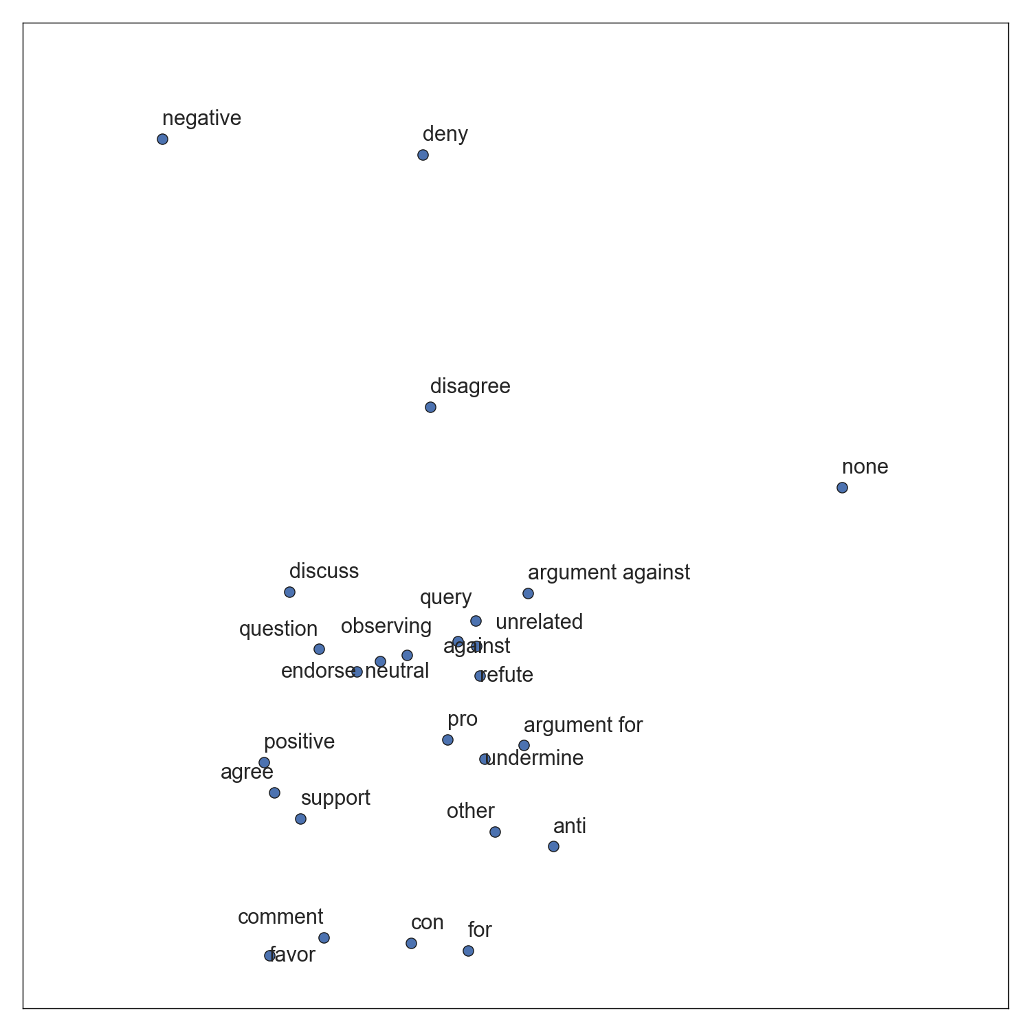
We examine the performance of soft mapping w/ fastText in more detail as they score the highest among other strong alternatives. Interestingly, the soft mappings benefit from splitting the predictions for the labels in the same group, such as wtwt__comment and all discuss-related, which leads to the better performance on perspectrum, poldeb, fnc1, argmin in comparison to the weak mappings. Nevertheless, this also introduces some errors. An illustrative example are short words – anti, pro, con, which are distant from all other label names in our pool (see Figure 5 in Appendix C for an illustration). The neighbourhoods are sometimes hard to interpret, e.g., con is not the closest word for any predicted labels in vast, and is aligned only with undermine, unrelated in ibmcs.
6 Discussion
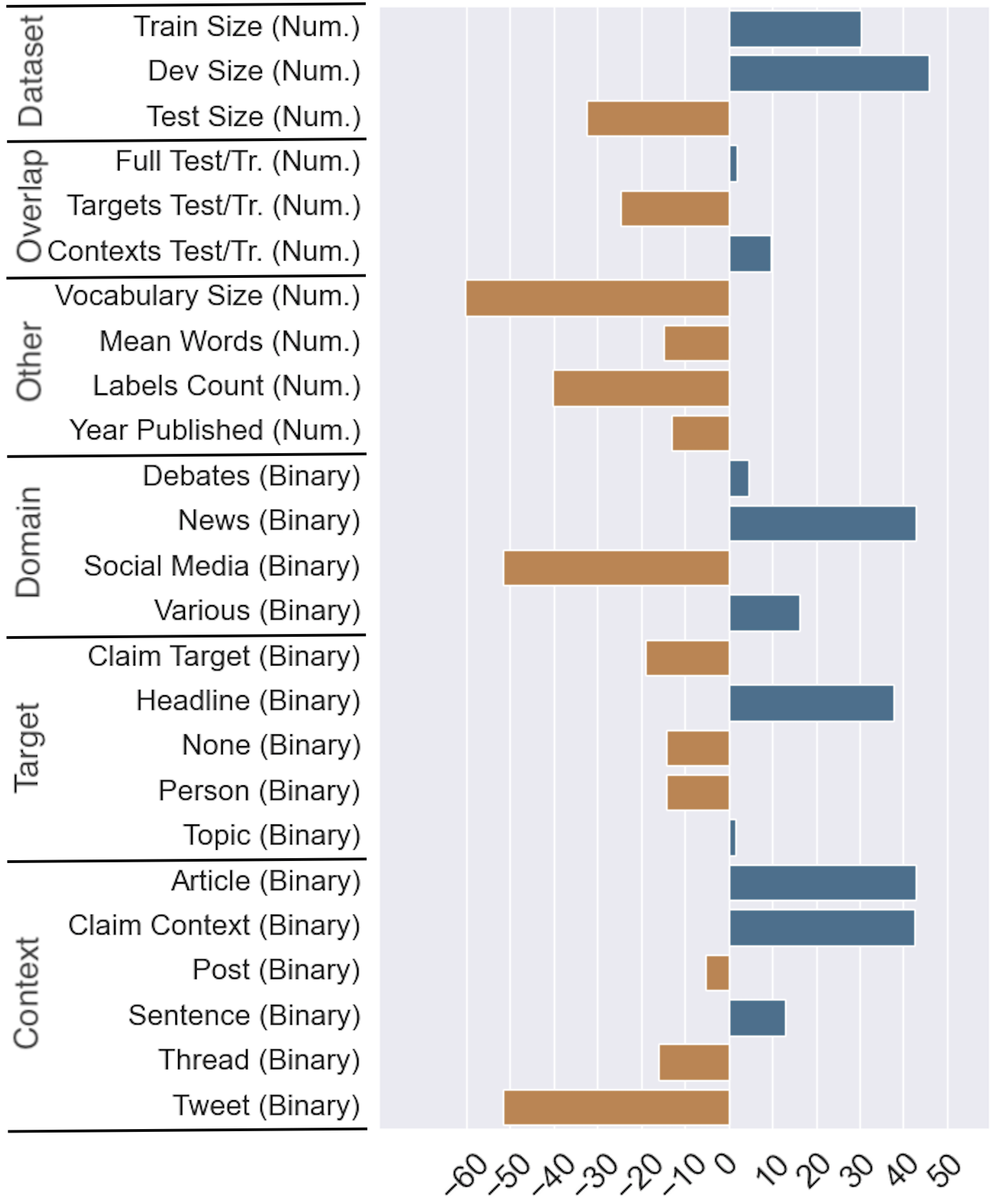
We further study the correlation between the scores for the best model in the out-of-domain setup MoLE w/ weak mappings and a rich set of quantitative and stance-related characteristics of the datasets (these are further discussed in Section 3 and in Appendix B). In particular, we represent each dataset as a set of features, e.g., fnc1 would have target – News, training set size of 42,476, etc., and then we measure the Pearson correlation between these features and the model’s F1 scores per dataset.
Figure 3 shows the most important factors for out-of-domain performance.777Some of the factors in the analysis are not independent, e.g., Social Media as a domain, and Tweet as a context. We see positive correlations of F1 with the training, and the development set sizes, and a negative one with the testing set size, which suggests that large datasets are indeed harder for the model. Interestingly, if there is an overlap in the targets between the testing and the training sets, the model’s F1 is worse; however, this is not true for context overlap. Unsurprisingly, the size of the vocabulary is a factor that negatively impacts F1, and its moderate negative correlation with the model’s scores confirms that.
The domain, the target and the context types are also important facets: the News domain has a sizable positive correlation with F1, which is also true for the related features Headline target and Article body. Another positive correlation is for having a Claim as the context. On the contrary, a key factor that hinders model performance is Social Media text, i.e., having a tweet as a context.
7 Conclusion and Future Work
We have proposed a novel end-to-end unsupervised framework for out-of-domain stance detection with respect to unseen labels. In particular, we combined domain adaptation techniques such as Mixture-of-Experts and domain-adversarial training with label embeddings, which yielded sizable performance gains on 16 datasets over strong baselines: both in-domain, i.e., for seen targets, and out-of-domain, i.e., for unseen targets. Moreover, we performed an exhaustive analysis of the cross-domain results, and we highlighted the most important factors influencing the model performance.
Acknowledgments
We thank the anonymous reviewers for their helpful questions and comments, which have helped us improve the quality of the paper.
We also would like to thank Guillaume Bouchard for the useful feedback. Finally, we thank the authors of the stance datasets for open-sourcing and providing us with their data.
Ethics and Broader Impact
Dataset Collection
We use publicly available datasets and we have no control over the way they were collected. For datasets that distributed their data as Twitter IDs, we used the Twitter API888http://developer.twitter.com/en/docs to obtain the full text of the tweets, which is in accordance with the terms of use outlined by Twitter.999http://developer.twitter.com/en/developer-terms/agreement-and-policy Note that we only downloaded public tweets.
Biases
We note that some of the annotations are subjective. Thus, it is inevitable that there would be certain biases in the datasets. These biases, in turn, will likely be exacerbated by the supervised models trained on them (Waseem et al., 2021). This is beyond our control, as are the potential biases in pre-trained large-scale transformers such as BERT and RoBERTa, which we use in our experiments.
Intended Use and Misuse Potential
Our models can enable analysis of text and social media content, which could be of interest to business, to fact-checkers, journalists, social media platforms, and policymakers. However, they could also be misused by malicious actors, especially as most of the datasets we consider in this paper are obtained from social media. Most datasets compiled from social media present some risk of misuse. We, therefore, ask researchers to exercise caution.
Environmental Impact
We would also like to note that the use of large-scale Transformers requires a lot of computations and the use of GPUs/TPUs for training, which contributes to global warming Strubell et al. (2019). This is a bit less of an issue in our case, as we do not train such models from scratch; rather, we fine-tune them on relatively small datasets. Moreover, running on a CPU for inference, once the model has been fine-tuned, is perfectly feasible, and CPUs contribute much less to global warming.
References
- Aharoni et al. (2014) Ehud Aharoni, Anatoly Polnarov, Tamar Lavee, Daniel Hershcovich, Ran Levy, Ruty Rinott, Dan Gutfreund, and Noam Slonim. 2014. A benchmark dataset for automatic detection of claims and evidence in the context of controversial topics. In Proceedings of the First Workshop on Argumentation Mining, ArgMining ’14, pages 64–68, Baltimore, Maryland, USA.
- Aldayel and Magdy (2019) Abeer Aldayel and Walid Magdy. 2019. Your stance is exposed! analysing possible factors for stance detection on social media. Proc. ACM Hum.-Comput. Interact., 3(CSCW).
- Allaway and McKeown (2020) Emily Allaway and Kathleen McKeown. 2020. Zero-Shot Stance Detection: A Dataset and Model using Generalized Topic Representations. In Proceedings of the 2020 Conference on Empirical Methods in Natural Language Processing, EMNLP ’20, pages 8913–8931, Online.
- Augenstein et al. (2019) Isabelle Augenstein, Christina Lioma, Dongsheng Wang, Lucas Chaves Lima, Casper Hansen, Christian Hansen, and Jakob Grue Simonsen. 2019. MultiFC: A real-world multi-domain dataset for evidence-based fact checking of claims. In Proceedings of the 2019 Conference on Empirical Methods in Natural Language Processing and the 9th International Joint Conference on Natural Language Processing, EMNLP-IJCNLP ’18, pages 4685–4697, Hong Kong, China.
- Augenstein et al. (2016) Isabelle Augenstein, Tim Rocktäschel, Andreas Vlachos, and Kalina Bontcheva. 2016. Stance detection with bidirectional conditional encoding. In Proceedings of the 2016 Conference on Empirical Methods in Natural Language Processing, EMNLP ’16, pages 876–885, Austin, Texas.
- Augenstein et al. (2018) Isabelle Augenstein, Sebastian Ruder, and Anders Søgaard. 2018. Multi-task learning of pairwise sequence classification tasks over disparate label spaces. In Proceedings of the 2018 Conference of the North American Chapter of the Association for Computational Linguistics: Human Language Technologies, NAACL-HLT ’18, pages 1896–1906, New Orleans, Louisiana, USA.
- Baly et al. (2018) Ramy Baly, Mitra Mohtarami, James Glass, Lluís Màrquez, Alessandro Moschitti, and Preslav Nakov. 2018. Integrating stance detection and fact checking in a unified corpus. In Proceedings of the 2018 Conference of the North American Chapter of the Association for Computational Linguistics: Human Language Technologies, NAACL-HLT ’18, pages 21–27, New Orleans, Louisiana, USA.
- Bar-Haim et al. (2017) Roy Bar-Haim, Indrajit Bhattacharya, Francesco Dinuzzo, Amrita Saha, and Noam Slonim. 2017. Stance classification of context-dependent claims. In Proceedings of the 15th Conference of the European Chapter of the Association for Computational Linguistics, EACL ’17, pages 251–261, Valencia, Spain.
- Barbieri et al. (2020) Francesco Barbieri, Jose Camacho-Collados, Luis Espinosa Anke, and Leonardo Neves. 2020. TweetEval: Unified benchmark and comparative evaluation for tweet classification. In Findings of the Association for Computational Linguistics: EMNLP 2020, EMNLP Findings ’20, pages 1644–1650, Online.
- Beryozkin et al. (2019) Genady Beryozkin, Yoel Drori, Oren Gilon, Tzvika Hartman, and Idan Szpektor. 2019. A joint named-entity recognizer for heterogeneous tag-sets using a tag hierarchy. In Proceedings of the 57th Annual Meeting of the Association for Computational Linguistics, ACL ’19, pages 140–150, Florence, Italy.
- Bjerva et al. (2020) Johannes Bjerva, Wouter Kouw, and Isabelle Augenstein. 2020. Back to the future – temporal adaptation of text representations. In Proceedings of the 34rd AAAI Conference on Artificial Intelligence, number 05 in AAAI ’20, pages 7440–7447, Honolulu, Hawaii, USA.
- Blitzer et al. (2006) John Blitzer, Ryan McDonald, and Fernando Pereira. 2006. Domain adaptation with structural correspondence learning. In Proceedings of the 2006 Conference on Empirical Methods in Natural Language Processing, EMNLP ’06, pages 120–128, Sydney, Australia.
- Boltužić and Šnajder (2014) Filip Boltužić and Jan Šnajder. 2014. Back up your stance: Recognizing arguments in online discussions. In Proceedings of the First Workshop on Argumentation Mining, ArgMining ’14, pages 49–58, Baltimore, Maryland, USA.
- Chai et al. (2020) Duo Chai, Wei Wu, Qinghong Han, Fei Wu, and Jiwei Li. 2020. Description based text classification with reinforcement learning. In Proceedings of the 37th International Conference on Machine Learning, volume 119 of ICLR ’20, pages 1371–1382, Virtual Event.
- Chang et al. (2020) Wei-Cheng Chang, Hsiang-Fu Yu, Kai Zhong, Yiming Yang, and Inderjit S. Dhillon. 2020. Taming pretrained transformers for extreme multi-label text classification. In Proceedings of the 26th ACM SIGKDD Conference on Knowledge Discovery and Data Mining, KDD ’20, pages 3163–3171, Virtual Event.
- Chen et al. (2019) Sihao Chen, Daniel Khashabi, Wenpeng Yin, Chris Callison-Burch, and Dan Roth. 2019. Seeing things from a different angle:discovering diverse perspectives about claims. In Proceedings of the 2019 Conference of the North American Chapter of the Association for Computational Linguistics: Human Language Technologies, NAACL-HLT ’17, pages 542–557, Minneapolis, Minnesota, USA.
- Conforti et al. (2020a) Costanza Conforti, Jakob Berndt, Mohammad Taher Pilehvar, Chryssi Giannitsarou, Flavio Toxvaerd, and Nigel Collier. 2020a. STANDER: An expert-annotated dataset for news stance detection and evidence retrieval. In Findings of the Association for Computational Linguistics: EMNLP 2020, EMNLP Findings ’20, pages 4086–4101, Online.
- Conforti et al. (2020b) Costanza Conforti, Jakob Berndt, Mohammad Taher Pilehvar, Chryssi Giannitsarou, Flavio Toxvaerd, and Nigel Collier. 2020b. Will-they-won’t-they: A very large dataset for stance detection on Twitter. In Proceedings of the 58th Annual Meeting of the Association for Computational Linguistics, ACL ’19, pages 1715–1724, Online.
- Darwish et al. (2020) Kareem Darwish, Peter Stefanov, Michaël Aupetit, and Preslav Nakov. 2020. Unsupervised user stance detection on twitter. Proceedings of the International AAAI Conference on Web and Social Media, 14(1):141–152.
- Daumé III (2007) Hal Daumé III. 2007. Frustratingly easy domain adaptation. In Proceedings of the 45th Annual Meeting of the Association of Computational Linguistics, ACL ’07, pages 256–263, Prague, Czech Republic.
- Devlin et al. (2019) Jacob Devlin, Ming-Wei Chang, Kenton Lee, and Kristina Toutanova. 2019. BERT: Pre-training of deep bidirectional transformers for language understanding. In Proceedings of the 2019 Conference of the North American Chapter of the Association for Computational Linguistics: Human Language Technologies, NAACL-HLT ’19, pages 4171–4186, Minneapolis, Minnesota, USA.
- Donahue et al. (2013) Jeff Donahue, Judy Hoffman, Erik Rodner, Kate Saenko, and Trevor Darrell. 2013. Semi-supervised domain adaptation with instance constraints. In 2013 IEEE Conference on Computer Vision and Pattern Recognition, CVPR ’13, pages 668–675, Portland, Oregon, USA.
- Ferreira and Vlachos (2016) William Ferreira and Andreas Vlachos. 2016. Emergent: a novel data-set for stance classification. In Proceedings of the 2016 Conference of the North American Chapter of the Association for Computational Linguistics: Human Language Technologies, NAACL-HLT ’16, pages 1163–1168, San Diego, California, USA.
- Finkel and Manning (2009) Jenny Rose Finkel and Christopher D. Manning. 2009. Hierarchical Bayesian domain adaptation. In Proceedings of Human Language Technologies: The 2009 Annual Conference of the North American Chapter of the Association for Computational Linguistics, NAACL-HLT ’09, pages 602–610, Boulder, Colorado.
- Ganin and Lempitsky (2015) Yaroslav Ganin and Victor S. Lempitsky. 2015. Unsupervised domain adaptation by backpropagation. In Proceedings of the 32nd International Conference on Machine Learning, volume 37 of ICML ’15, pages 1180–1189, Lille, France.
- Ganin et al. (2016) Yaroslav Ganin, Evgeniya Ustinova, Hana Ajakan, Pascal Germain, Hugo Larochelle, François Laviolette, Mario Marchand, and Victor Lempitsky. 2016. Domain-adversarial training of neural networks. Journal of Machine Learning Research, 17(1):2096–2030.
- Glandt et al. (2021) Kyle Glandt, Sarthak Khanal, Yingjie Li, Doina Caragea, and Cornelia Caragea. 2021. Stance detection in COVID-19 tweets. In Proceedings of the 59th Annual Meeting of the Association for Computational Linguistics and the 11th International Joint Conference on Natural Language Processing, ACL-IJCNLP ’21, pages 1596–1611, Online.
- Gorrell et al. (2019) Genevieve Gorrell, Elena Kochkina, Maria Liakata, Ahmet Aker, Arkaitz Zubiaga, Kalina Bontcheva, and Leon Derczynski. 2019. SemEval-2019 task 7: RumourEval, determining rumour veracity and support for rumours. In Proceedings of the 13th International Workshop on Semantic Evaluation, SemEval ’19, pages 845–854, Minneapolis, Minnesota, USA.
- Gui et al. (2017) Tao Gui, Qi Zhang, Haoran Huang, Minlong Peng, and Xuanjing Huang. 2017. Part-of-speech tagging for Twitter with adversarial neural networks. In Proceedings of the 2017 Conference on Empirical Methods in Natural Language Processing, EMNLP ’17, pages 2411–2420, Copenhagen, Denmark.
- Guo et al. (2018) Jiang Guo, Darsh Shah, and Regina Barzilay. 2018. Multi-source domain adaptation with mixture of experts. In Proceedings of the 2018 Conference on Empirical Methods in Natural Language Processing, EMNLP ’18, pages 4694–4703, Brussels, Belgium.
- Gururangan et al. (2020) Suchin Gururangan, Ana Marasović, Swabha Swayamdipta, Kyle Lo, Iz Beltagy, Doug Downey, and Noah A. Smith. 2020. Don’t stop pretraining: Adapt language models to domains and tasks. In Proceedings of the 58th Annual Meeting of the Association for Computational Linguistics, ACL ’20, pages 8342–8360, Online.
- Habernal et al. (2018) Ivan Habernal, Henning Wachsmuth, Iryna Gurevych, and Benno Stein. 2018. The argument reasoning comprehension task: Identification and reconstruction of implicit warrants. In Proceedings of the 2018 Conference of the North American Chapter of the Association for Computational Linguistics: Human Language Technologies, NAACL-HLT ’18, pages 1930–1940, New Orleans, Louisiana, USA.
- Han and Eisenstein (2019) Xiaochuang Han and Jacob Eisenstein. 2019. Unsupervised domain adaptation of contextualized embeddings for sequence labeling. In Proceedings of the 2019 Conference on Empirical Methods in Natural Language Processing and the 9th International Joint Conference on Natural Language Processing, EMNLP-IJCNLP ’19, pages 4238–4248, Hong Kong, China.
- Hanselowski et al. (2018) Andreas Hanselowski, Avinesh PVS, Benjamin Schiller, Felix Caspelherr, Debanjan Chaudhuri, Christian M. Meyer, and Iryna Gurevych. 2018. A retrospective analysis of the fake news challenge stance-detection task. In Proceedings of the 27th International Conference on Computational Linguistics, CoNLL ’18, pages 1859–1874, Santa Fe, New Mexico, USA.
- Hanselowski et al. (2019) Andreas Hanselowski, Christian Stab, Claudia Schulz, Zile Li, and Iryna Gurevych. 2019. A richly annotated corpus for different tasks in automated fact-checking. In Proceedings of the 23rd Conference on Computational Natural Language Learning, CoNLL ’19, pages 493–503, Hong Kong, China.
- Hardalov et al. (2021a) Momchil Hardalov, Arnav Arora, Preslav Nakov, and Isabelle Augenstein. 2021a. Few-shot cross-lingual stance detection with sentiment-based pre-training. arXiv.
- Hardalov et al. (2021b) Momchil Hardalov, Arnav Arora, Preslav Nakov, and Isabelle Augenstein. 2021b. A survey on stance detection for mis- and disinformation identification. arXiv preprint arXiv:2103.00242.
- Hasan and Ng (2013) Kazi Saidul Hasan and Vincent Ng. 2013. Stance classification of ideological debates: Data, models, features, and constraints. In Proceedings of the Sixth International Joint Conference on Natural Language Processing, IJCNLP ’13, pages 1348–1356, Nagoya, Japan.
- Hasan and Ng (2014) Kazi Saidul Hasan and Vincent Ng. 2014. Why are you taking this stance? Identifying and classifying reasons in ideological debates. In Proceedings of the 2014 Conference on Empirical Methods in Natural Language Processing, EMNLP ’14, pages 751–762, Doha, Qatar.
- Hossain et al. (2020) Tamanna Hossain, Robert L. Logan IV, Arjuna Ugarte, Yoshitomo Matsubara, Sean Young, and Sameer Singh. 2020. COVIDLies: Detecting COVID-19 misinformation on social media. In Proceedings of the 1st Workshop on NLP for COVID-19 (Part 2) at EMNLP 2020, NLP-COVID19 ’20, Online.
- Joulin et al. (2017) Armand Joulin, Edouard Grave, Piotr Bojanowski, and Tomas Mikolov. 2017. Bag of tricks for efficient text classification. In Proceedings of the 15th Conference of the European Chapter of the Association for Computational Linguistics, EACL ’17, pages 427–431, Valencia, Spain.
- Kingma and Ba (2015) Diederik P. Kingma and Jimmy Ba. 2015. Adam: A method for stochastic optimization. In 3rd International Conference on Learning Representations, ICLR ’15, San Diego, California, USA.
- Küçük and Can (2020) Dilek Küçük and Fazli Can. 2020. Stance detection: A survey. ACM Computing Surveys, 53(1).
- Kudo and Richardson (2018) Taku Kudo and John Richardson. 2018. SentencePiece: A simple and language independent subword tokenizer and detokenizer for neural text processing. In Proceedings of the 2018 Conference on Empirical Methods in Natural Language Processing: System Demonstrations, EMNLP ’18, pages 66–71, Brussels, Belgium.
- Li et al. (2018) Yitong Li, Timothy Baldwin, and Trevor Cohn. 2018. What’s in a domain? Learning domain-robust text representations using adversarial training. In Proceedings of the 2018 Conference of the North American Chapter of the Association for Computational Linguistics, NAACL-HLT ’18, pages 474–479, New Orleans, Louisiana, USA.
- Lin and Lu (2018) Bill Yuchen Lin and Wei Lu. 2018. Neural adaptation layers for cross-domain named entity recognition. In Proceedings of the 2018 Conference on Empirical Methods in Natural Language Processing, EMNLP ’18, pages 2012–2022, Brussels, Belgium.
- Lin et al. (2020) Chen Lin, Steven Bethard, Dmitriy Dligach, Farig Sadeque, Guergana Savova, and Timothy A Miller. 2020. Does BERT need domain adaptation for clinical negation detection? Journal of the American Medical Informatics Association, 27(4):584–591.
- Lipton et al. (2018) Zachary C. Lipton, Yu-Xiang Wang, and Alexander J. Smola. 2018. Detecting and correcting for label shift with black box predictors. In Proceedings of the 35th International Conference on Machine Learning, volume 80 of ICML ’18, pages 3128–3136, Stockholm, Sweden.
- Liu et al. (2019) Yinhan Liu, Myle Ott, Naman Goyal, Jingfei Du, Mandar Joshi, Danqi Chen, Omer Levy, Mike Lewis, Luke Zettlemoyer, and Veselin Stoyanov. 2019. RoBERTa: A robustly optimized BERT pretraining approach. arXiv:1907.11692.
- Loper and Bird (2002) Edward Loper and Steven Bird. 2002. NLTK: The natural language toolkit. In Proceedings of the ACL Workshop on Effective Tools and Methodologies for Teaching Natural Language Processing and Computational Linguistics, TeachingNLP ’02, pages 63–70, Philadelphia, Pennsylvania, USA.
- Ma et al. (2019) Xiaofei Ma, Peng Xu, Zhiguo Wang, Ramesh Nallapati, and Bing Xiang. 2019. Domain adaptation with BERT-based domain classification and data selection. In Proceedings of the 2nd Workshop on Deep Learning Approaches for Low-Resource NLP, DeepLo ’19, pages 76–83, Hong Kong, China.
- Mohammad et al. (2016) Saif Mohammad, Svetlana Kiritchenko, Parinaz Sobhani, Xiaodan Zhu, and Colin Cherry. 2016. SemEval-2016 task 6: Detecting stance in tweets. In Proceedings of the 10th International Workshop on Semantic Evaluation, SemEval ’16, pages 31–41, San Diego, California, USA.
- Mohammad et al. (2017) Saif M. Mohammad, Parinaz Sobhani, and Svetlana Kiritchenko. 2017. Stance and sentiment in tweets. ACM Transactions on Internet Technology, 17(3).
- Mohtarami et al. (2018) Mitra Mohtarami, Ramy Baly, James Glass, Preslav Nakov, Lluís Màrquez, and Alessandro Moschitti. 2018. Automatic stance detection using end-to-end memory networks. In Proceedings of the 2018 Conference of the North American Chapter of the Association for Computational Linguistics: Human Language Technologies, NAACL ’18, pages 767–776, New Orleans, Louisiana.
- Mohtarami et al. (2019) Mitra Mohtarami, James Glass, and Preslav Nakov. 2019. Contrastive language adaptation for cross-lingual stance detection. In Proceedings of the 2019 Conference on Empirical Methods in Natural Language Processing and the 9th International Joint Conference on Natural Language Processing, EMNLP-IJCNLP ’19, pages 4442–4452, Hong Kong, China.
- Mou et al. (2016) Lili Mou, Zhao Meng, Rui Yan, Ge Li, Yan Xu, Lu Zhang, and Zhi Jin. 2016. How transferable are neural networks in NLP applications? In Proceedings of the 2016 Conference on Empirical Methods in Natural Language Processing, EMNLP ’16, pages 479–489, Austin, Texas, USA.
- Pappas and Henderson (2019) Nikolaos Pappas and James Henderson. 2019. GILE: A generalized input-label embedding for text classification. Transactions of the Association for Computational Linguistics, 7:139–155.
- Paszke et al. (2019) Adam Paszke, Sam Gross, Francisco Massa, Adam Lerer, James Bradbury, Gregory Chanan, Trevor Killeen, Zeming Lin, Natalia Gimelshein, Luca Antiga, Alban Desmaison, Andreas Kopf, Edward Yang, Zachary DeVito, Martin Raison, Alykhan Tejani, Sasank Chilamkurthy, Benoit Steiner, Lu Fang, Junjie Bai, and Soumith Chintala. 2019. PyTorch: An imperative style, high-performance deep learning library. In Advances in Neural Information Processing Systems 30: Annual Conference on Neural Information Processing Systems 2017, NeurIPS ’19, pages 8024–8035.
- Pennington et al. (2014) Jeffrey Pennington, Richard Socher, and Christopher Manning. 2014. GloVe: Global vectors for word representation. In Proceedings of the 2014 Conference on Empirical Methods in Natural Language Processing, EMNLP ’14, pages 1532–1543, Doha, Qatar.
- Pomerleau and Rao (2017) Dean Pomerleau and Delip Rao. 2017. Fake news challenge stage 1 (FNC-I): Stance detection.
- Qazvinian et al. (2011) Vahed Qazvinian, Emily Rosengren, Dragomir R. Radev, and Qiaozhu Mei. 2011. Rumor has it: Identifying misinformation in microblogs. In Proceedings of the 2011 Conference on Empirical Methods in Natural Language Processing, EMNLP ’11, pages 1589–1599, Edinburgh, Scotland, UK.
- Rethmeier and Augenstein (2020) Nils Rethmeier and Isabelle Augenstein. 2020. Data-efficient pretraining via contrastive self-supervision. arXiv preprint arXiv:2010.01061.
- Rietzler et al. (2020) Alexander Rietzler, Sebastian Stabinger, Paul Opitz, and Stefan Engl. 2020. Adapt or get left behind: Domain adaptation through BERT language model finetuning for aspect-target sentiment classification. In Proceedings of the 12th Language Resources and Evaluation Conference, LREC ’20, pages 4933–4941, Marseille, France.
- Schiller et al. (2021) Benjamin Schiller, Johannes Daxenberger, and Iryna Gurevych. 2021. Stance detection benchmark: How robust is your stance detection? KI-Künstliche Intelligenz, pages 1–13.
- Shah et al. (2018) Darsh Shah, Tao Lei, Alessandro Moschitti, Salvatore Romeo, and Preslav Nakov. 2018. Adversarial domain adaptation for duplicate question detection. In Proceedings of the 2018 Conference on Empirical Methods in Natural Language Processing, EMNLP ’18, pages 1056–1063, Brussels, Belgium.
- Sobhani et al. (2015) Parinaz Sobhani, Diana Inkpen, and Stan Matwin. 2015. From argumentation mining to stance classification. In Proceedings of the 2nd Workshop on Argumentation Mining, ArgMining ’15, pages 67–77, Denver, Colorado, USA.
- Sobhani et al. (2017) Parinaz Sobhani, Diana Inkpen, and Xiaodan Zhu. 2017. A dataset for multi-target stance detection. In Proceedings of the 15th Conference of the European Chapter of the Association for Computational Linguistics, EACL ’17, pages 551–557, Valencia, Spain.
- Somasundaran and Wiebe (2009) Swapna Somasundaran and Janyce Wiebe. 2009. Recognizing stances in online debates. In Proceedings of the Joint Conference of the 47th Annual Meeting of the ACL and the 4th International Joint Conference on Natural Language Processing of the AFNLP, ACL-AFNLP ’09, pages 226–234, Suntec, Singapore.
- Somasundaran and Wiebe (2010) Swapna Somasundaran and Janyce Wiebe. 2010. Recognizing stances in ideological on-line debates. In Proceedings of the NAACL-HLT 2010 Workshop on Computational Approaches to Analysis and Generation of Emotion in Text, CAAGET ’10, pages 116–124, Los Angeles, California, USA.
- Stab et al. (2018) Christian Stab, Tristan Miller, Benjamin Schiller, Pranav Rai, and Iryna Gurevych. 2018. Cross-topic argument mining from heterogeneous sources. In Proceedings of the 2018 Conference on Empirical Methods in Natural Language Processing, EMNLP ’18, pages 3664–3674, Brussels, Belgium.
- Stefanov et al. (2020) Peter Stefanov, Kareem Darwish, Atanas Atanasov, and Preslav Nakov. 2020. Predicting the topical stance and political leaning of media using tweets. In Proceedings of the 58th Annual Meeting of the Association for Computational Linguistics, ACL ’20, pages 527–537, Online.
- Strubell et al. (2019) Emma Strubell, Ananya Ganesh, and Andrew McCallum. 2019. Energy and policy considerations for deep learning in NLP. In Proceedings of the 57th Annual Meeting of the Association for Computational Linguistics, ACL ’19, pages 3645–3650, Florence, Italy.
- Tang et al. (2014) Duyu Tang, Furu Wei, Nan Yang, Ming Zhou, Ting Liu, and Bing Qin. 2014. Learning sentiment-specific word embedding for Twitter sentiment classification. In Proceedings of the 52nd Annual Meeting of the Association for Computational Linguistics, ACL ’14, pages 1555–1565, Baltimore, Maryland, USA.
- van der Maaten and Hinton (2008) Laurens van der Maaten and Geoffrey Hinton. 2008. Visualizing data using t-SNE. Journal of Machine Learning Research, 9(86):2579–2605.
- Vaswani et al. (2017) Ashish Vaswani, Noam Shazeer, Niki Parmar, Jakob Uszkoreit, Llion Jones, Aidan N. Gomez, Lukasz Kaiser, and Illia Polosukhin. 2017. Attention is all you need. In Advances in Neural Information Processing Systems 30: Annual Conference on Neural Information Processing Systems 2017, NIPS ’17, pages 5998–6008, Long Beach, California, USA.
- Walker et al. (2012) Marilyn Walker, Jean Fox Tree, Pranav Anand, Rob Abbott, and Joseph King. 2012. A corpus for research on deliberation and debate. In Proceedings of the Eighth International Conference on Language Resources and Evaluation, LREC ’12, pages 812–817, Istanbul, Turkey.
- Wang et al. (2019) Rui Wang, Deyu Zhou, Mingmin Jiang, Jiasheng Si, and Y. Yang. 2019. A survey on opinion mining: From stance to product aspect. IEEE Access, 7:41101–41124.
- Waseem et al. (2021) Zeerak Waseem, Smarika Lulz, Joachim Bingel, and Isabelle Augenstein. 2021. Disembodied machine learning: On the illusion of objectivity in NLP. arXiv:2101.11974.
- Wolf et al. (2020) Thomas Wolf, Lysandre Debut, Victor Sanh, Julien Chaumond, Clement Delangue, Anthony Moi, Pierric Cistac, Tim Rault, Remi Louf, Morgan Funtowicz, Joe Davison, Sam Shleifer, Patrick von Platen, Clara Ma, Yacine Jernite, Julien Plu, Canwen Xu, Teven Le Scao, Sylvain Gugger, Mariama Drame, Quentin Lhoest, and Alexander Rush. 2020. Transformers: State-of-the-art natural language processing. In Proceedings of the 2020 Conference on Empirical Methods in Natural Language Processing: System Demonstrations, EMNLP ’20, pages 38–45, Online.
- Wright and Augenstein (2020) Dustin Wright and Isabelle Augenstein. 2020. Transformer based multi-source domain adaptation. In Proceedings of the 2020 Conference on Empirical Methods in Natural Language Processing, EMNLP ’20, pages 7963–7974, Online.
- Yao et al. (2015) Ting Yao, Yingwei Pan, Chong-Wah Ngo, Houqiang Li, and Tao Mei. 2015. Semi-supervised domain adaptation with subspace learning for visual recognition. In IEEE Conference on Computer Vision and Pattern Recognition, CVPR ’15, pages 2142–2150, Boston, Massachusetts, USA.
- Zhang et al. (2018) Honglun Zhang, Liqiang Xiao, Wenqing Chen, Yongkun Wang, and Yaohui Jin. 2018. Multi-task label embedding for text classification. In Proceedings of the 2018 Conference on Empirical Methods in Natural Language Processing, EMNLP ’18, pages 4545–4553, Brussels, Belgium.
- Zubiaga (2018) Arkaitz Zubiaga. 2018. A longitudinal assessment of the persistence of Twitter datasets. Journal of the Association for Information Science and Technology, 69(8):974–984.
- Zubiaga et al. (2018) Arkaitz Zubiaga, Ahmet Aker, Kalina Bontcheva, Maria Liakata, and Rob Procter. 2018. Detection and resolution of rumours in social media: A survey. ACM Computing Surveys, 51(2).
| Dataset | Target | Context | Label |
| arc | States do not need special schools for the deaf | In the early 90’s I was studying Maths of Finance at university and fees and charges were just starting to raise their ugly heads. In hindsight Australia is about 20 years ahead of the US with … | unrelated |
| argmin | cloning | In Humanity Enhanced , I challenge the idea that children conceived through SCNT would have their autonomy violated – or would somehow lack or lose autonomy – in any sense inapplicable to “ ordinary ” children . | argument_for |
| emergent | Jess Smith of Chatham, Kent was the smiling sun baby in the Teletubbies TV show | Canterbury Christ Church University student Jess Smith, from Chatham, starred as Teletubbies sun | for |
| fnc1 | Nigeria announces truce with Boko Haram; fate of schoolgirls unclear | Well, here’s the creepiest thing you’ll read all day. Australian Dylan Thomas found a tropical spider burrowed UNDER his skin after returning from a trip to Bali. … | unrelated |
| iac1 | marijuana legalization |
[P1] Instead of rewriting what I have already written numerous times, I will post a copy of a recent post I made on another thread regarding this same topic. You can find the original post here.
[P2] I enjoy the experience of getting drunk, high, or anything else like that…… |
pro |
| ibmcs | This house believes atheism is the only way | God is improbable | pro |
| mtsd | Hilary Clinton | Love that #democratic primary is talking bout real issues #BernieSanders made a great case now let’s hear from #HillaryClinton #DemTownHall | none |
| perspectrum | The lack of investment in teachers is the greatest barrier to achieving universal primary education | It should be social policy to make teaching careers more desirable | support |
| poldeb | should the us have universal healthcare | Yes, my posts all turned up backward because I replied in the order I read.Props for all the research you did. I still wholeheartedly disagree.Here’s one article I came across that summarizes my entire point of view. http://url In the end, perhaps we agree to disagree … | against |
| rumor | Sarah Palin getting divorced? | OneRiot.com - Palin Denies First Dude Divorce Rumors http://url | deny |
| scd | – | First off, the only people that want to legalize pot are the liberals that sit around all day, living off wellfare and smoke drugs. They do this because they are to uneducated to get a job, and figure the liberal … | against |
| semeval2016t6 | Legalization of Abortion | @mrsdrjim did you know #wrp @BrianJeanWRP tried to get personhood going via federal #motion312. #SemST | none |
| semeval2019t7 | – | Wow, that is fascinating! I hope you never mock our proud Scandi heritage again. | comment |
| snopes | president-elect donald trump’s inauguration will be the first presidential inauguration that rep. john lewis has skipped. | wrong (or lie)! | refute |
| vast | public education | Public schools are the entire country’s investment in an educated populace. They are our investment in a responsible, civil society. Everyone benefits when every citizen is able to read, write, understand history … | pro |
| wtwt | Anthem acquires Cigna | - #tuu i #yoo - Anthem Reaffirms Commitment to Its $47-Billion Bid for Cigna: Anthem stands by its $47-bill… http://url | support |
Appendix A Fine-Tuning and Hyper-Parameters
- •
-
•
All models use Adam (Kingma and Ba, 2015) with weight decay 1e-8, 0.9, 0.999, 1e-08, and are trained for five epochs with batch size 64, and maximum length of 100 tokens.101010When needed, we truncated the sequences token by token, starting from the longest sequence in the pair.
- •
-
•
The values of the hyper-parameters were selected on the development set.
-
•
We chose the best model checkpoint based on the performance on the development set.
-
•
For the MTL/MoE models, we sampled each batch from a single randomly selected dataset/domain.
-
•
We used the same seed for all experiments.
-
•
Each experiment took around 1h 15m on a single NVIDIA V100 GPU using half precision.
-
•
For logistic regression, we converted the text to lowercase, removed the stop words, and limited the dictionary in the TF.IDF to 15,000 unigrams. We built the vocabulary using the concatenated target and context. The target and the context were transformed separately and concatenated to form the input vector.
Appendix B Dataset Analysis
B.1 Data Splits
We could not reconstruct some of the Social Media datasets in full (marked with a * symbol in Table 2), as with only tweet IDs, we could not obtain the actual tweet text in some cases. This is a known phenomenon in Twitter: with time, older tweets become unavailable for various reasons, such as tweets/accounts being deleted or accounts being made private (Zubiaga, 2018). The missing tweets were evenly distributed among the splits of the datasets except for rumor, where we chose a topic for the test set for which all example texts were available.
Here, we provide more detail about the splits we used for the datasets, in cases where there is a deviation from the original. For the datasets in common, we used the splitting by Schiller et al. (2021). We further tried to enforce a larger domain diversity between the training, the development, and the testing sets; hereby, we put (whenever possible) all examples from a particular topic (domain) strictly into a single split.
argmin
We removed all non-arguments. The training, the development, and the test data splits consist of five, one, and two topics, respectively.
iac1
Split with no intersection of topics between the training, the development, and the testing sets.
ibmcs
Pre-defined training and testing splits. We further reserved 10% of the training data for development set.
mtsd
We used the pre-defined splits, but we created two pairs for each example: a positive and a negative one with respect to the target.
poledb
We used the domains Healthcare, Guns, Gay Rights and God for training, Abortion for development, and Creation for testing.
rumor
We used the airfrance rumour for our test set, and we split the remaining data in ratio 9:1 for training and development, respectively.
wtwt
We used DIS_FOXA operation for testing, AET_HUM for development, and the rest for training. To standardize the targets, we rewrote them as sentences, i.e., company X acquires company Y.
scd
We used a split with Marijuana for development, Obama for testing, and the rest for training.
semeval2016t6
We split it to increase the size of the development set.
snopes
We adjusted the splits for compatibility with the stance setup. We further extracted and converted the rumours and their evidence into target–context pairs.
| Dev | Test | |||||
| % of split in Train | F | T | C | F | T | C |
| arc | 1.9 | 100.0 | 93.7 | 1.5 | 100.0 | 93.8 |
| iac1 | 0.0 | 0.0 | 0.2 | 0.0 | 0.0 | 0.1 |
| perspectrum | 1.5 | 1.5 | 37.2 | 0.0 | 0.0 | 26.4 |
| poldeb | 0.0 | 0.0 | 0.0 | 0.0 | 0.0 | 0.0 |
| scd | — | — | 0.0 | — | — | 0.0 |
| emergent | 0.0 | 0.0 | 3.0 | 0.0 | 0.0 | 1.7 |
| fnc1 | 1.7 | 100.0 | 99.8 | 0.0 | 0.6 | 0.9 |
| snopes | 0.0 | 0.0 | 0.0 | 0.0 | 0.0 | 0.3 |
| mtsd | 0.8 | 100.0 | 1.5 | 0.3 | 100.0 | 0.5 |
| rumor | 17.6 | 100.0 | 17.6 | 0.0 | 0.0 | 0.0 |
| semeval2016t6 | 0.0 | 100.0 | 0.0 | 0.0 | 100.0 | 0.0 |
| semeval2019t7 | — | — | 1.4 | — | — | 4.8 |
| wtwt | 0.0 | 0.0 | 11.4 | 0.0 | 0.0 | 0.0 |
| argmin | 0.0 | 0.0 | 0.0 | 0.0 | 0.0 | 0.0 |
| ibmcs | 0.0 | 100.0 | 1.0 | 0.0 | 0.0 | 0.2 |
| vast | 0.0 | 43.6 | 0.0 | 0.0 | 49.5 | 0.0 |
| Tokenization | Words | Tokens (Words) | Tokens | ||
| Unique | Mean | 25% | Median | Max | |
| arc | 27,835 | 126.0 (118.3) | 84 | 116 | 286 |
| argmin | 17,990 | 30.6 (28.6) | 20 | 28 | 208 |
| emergent | 6,940 | 27.6 (23.1) | 22 | 26 | 111 |
| fnc1 | 40,738 | 503.2 (432.2) | 279 | 413 | 6,182 |
| iac1 | 88,478 | 1,554.7 (1,347.9) | 132 | 390 | 104,034 |
| ibmcs | 5,007 | 23.4 (21.9) | 18 | 23 | 55 |
| mtsd | 9,799 | 36.3 (25.9) | 33 | 36 | 65 |
| perspectrum | 9,999 | 22.4 (20.4) | 17 | 21 | 75 |
| poldeb | 40,422 | 178.0 (160.6) | 55 | 112 | 2,144 |
| rumor | 15,801 | 38.4 (24.4) | 32 | 39 | 78 |
| scd | 23,592 | 151.4 (134.8) | 39 | 78 | 6,358 |
| semeval2016t6 | 15,016 | 32.8 (22.1) | 28 | 33 | 68 |
| semeval2019t7 | 20,789 | 33.5 (22.0) | 17 | 27 | 1,466 |
| snopes | 33,896 | 53.4 (45.5) | 40 | 51 | 327 |
| vast | 24,644 | 123.2 (115.7) | 80 | 114 | 271 |
| wtwt | 102,672 | 45.7 (23.1) | 39 | 46 | 193 |
B.2 Overlap Statistics
Next, in Table 8, we examine the proportion of contexts and targets from the development and the testing datasets that are also present in the training split. We did not change the original data in any way, and we used the splits as described in Section B.1.
Table 8 further shows statistics about the datasets in terms of the number of words and sub-words they contain (see Table 9). The first column in the table shows the number of unique tokens (word types) in each dataset after tokenisation using NLTK’s casual tokeniser (Loper and Bird, 2002), which retains the casing of the words; thus word types of different casing are counted separately. We observe that the datasets with the largest vocabularies are those (i) with higher numbers of examples (fnc1 and wtwt), (ii) whose contexts are threads rather than single posts (iac1 has over 1,300 words on average), and (iii) that cover diverse topics such as poldeb with six unrelated ones. In contrast, small or narrow datasets such as ibmcs have the smallest vocabularies (fewer than 5,000 words).
In the subsequent columns, we report statistics in terms of number of sub-words (i.e., SentencePieces (Kudo and Richardson, 2018) from RoBERTaBase’s tokeniser). With that, we want to present the expected coverage in terms of tokens for a pre-trained model. On average, most of the datasets are well under 100 tokens in length, which is commonly observed for tweets,111111Tweets have a strict character limit. Depending on the time period, this limit can vary. but some datasets have a higher average number of tokens, e.g., debate-related datasets such as arc, poldeb, scd, vast fit in 200 tokens on average, which is also the case for datasets containing large news articles or use social media threads as context (fnc1, iac1), where the average length is over 500.
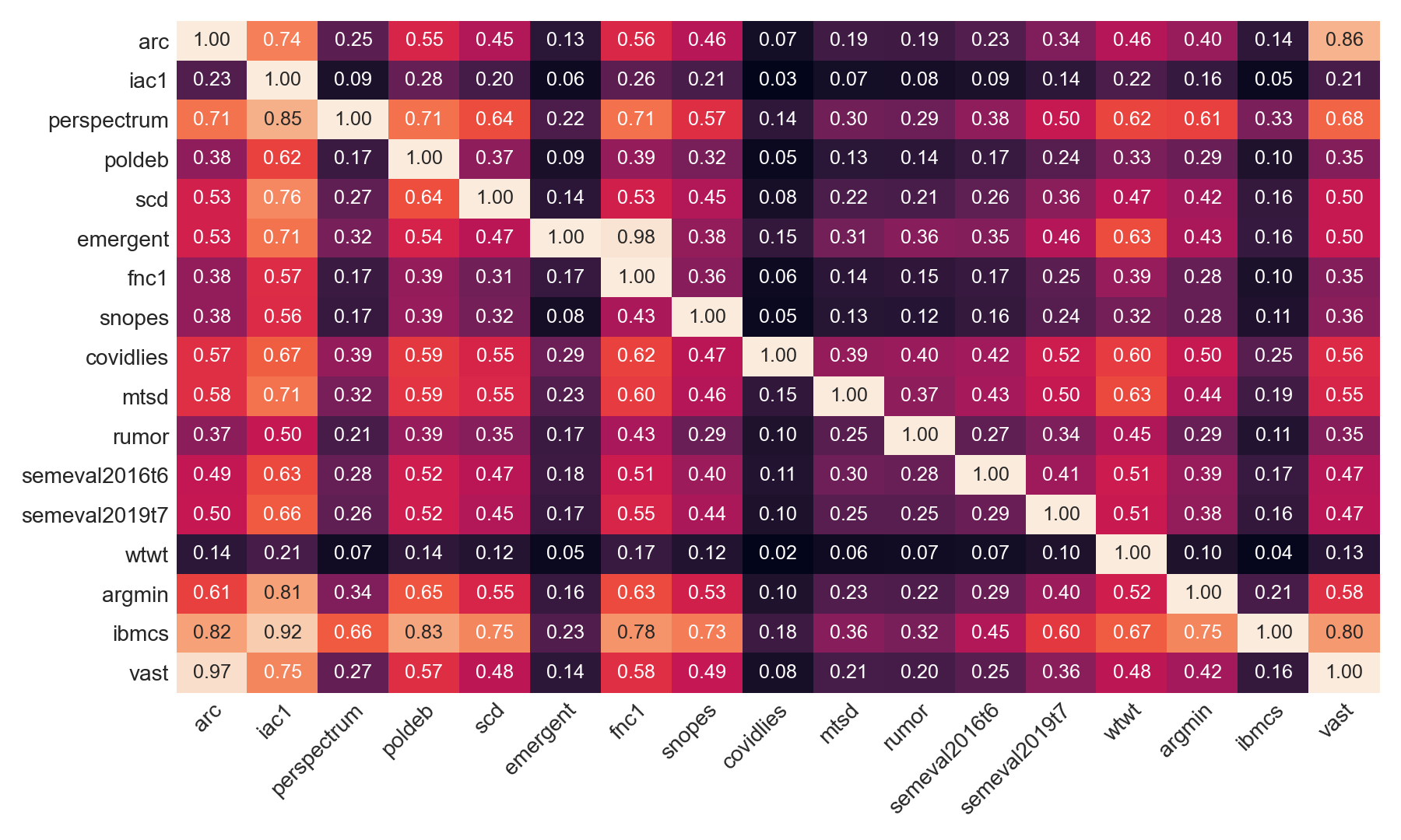
Finally, Figure 4 shows the relative word overlap between datasets. The numbers in each cell shows how much of the word types in dataset (row) are contained in the dataset (column). For example, in the first column in the last row (vast arc), we see that 97% of the words in vast are also present in arc. Similarly, in the first row and the last column, we see that 86% of the words in arc are also in vast. Note that we sort the columns and the rows by their sources (see Table 1). We can see that datasets with the largest vocabularies (iac1 and wtwt) have low overlap with other datasets, including with each other, up to 28% only (row-wise).
When looking at how many words in other datasets are contained in them (column-wise), we see that iac1 has 50% or more vocabulary overlap with the other datasets, even with ones from different sources. Then, wtwt’s overlaps are 30–70%, which is expected as its texts are from social media and cover a single topic (company acquisitions). For datasets that are either small or cover few topics (emergant, ibmcs, perspectrum), we see that moderate to large part of their vocabularies is contained in other datasets; yet, the opposite in not true. Moreover, social media datasets are orthogonal to each other, with cross-overlaps of up to 50% (both row-wise and column-wise), except for wtwt. This is also seen when measuring how much of other datasets’ vocabulary they contain (column-wise).


Appendix C Embedding Label Spaces
Here, we present the embeddings based on the labels’ names. We explore five sets of embeddings: (i) well-established ones such as fastText (Joulin et al., 2017), GloVe (Pennington et al., 2014), and RoBERTa (Liu et al., 2019), and (ii) sentiment-enriched ones like Sentiment-specific word embedding (SSWE) (Tang et al., 2014) and RoBERTa Twitter Sentiment (roberta-sentiment) (Barbieri et al., 2020). Our motivation for including the latter is that the names of the stance labels are often sentiment-related, and thus encoding that information into the latent space could yield better grouping. We encode each label with the corresponding word from the embedding’s directory for non-contextualized embeddings, if the name contains multiple words, e.g., argument for, then we split on white space, and we take the average of each word’s embeddings. For RoBERTa-based models, we take the representation from the [CLS] token. Finally, we project the obtained vectors into two dimensions using PCA. The resulting plots are shown in Figure 5.