Symbolic Time and Space Tradeoffs for Probabilistic Verification

Abstract

We present a faster symbolic algorithm for the following central problem in probabilistic verification: Compute the maximal end-component (MEC) decomposition of Markov decision processes (MDPs). This problem generalizes the SCC decomposition problem of graphs and closed recurrent sets of Markov chains. The model of symbolic algorithms is widely used in formal verification and model-checking, where access to the input model is restricted to only symbolic operations (e.g., basic set operations and computation of one-step neighborhood). For an input MDP with $n$ vertices and $m$ edges, the classical symbolic algorithm from the 1990s for the MEC decomposition requires $O(n^{2})$ symbolic operations and $O(1)$ symbolic space. The only other symbolic algorithm for the MEC decomposition requires $O(n\sqrt{m})$ symbolic operations and $O(\sqrt{m})$ symbolic space. The main open question has been whether the worst-case $O(n^{2})$ bound for symbolic operations can be beaten for MEC decomposition computation. In this work, we answer the open question in affirmative. We present a symbolic algorithm that requires $\widetilde{O}(n^{1.5})$ symbolic operations and $\widetilde{O}(\sqrt{n})$ symbolic space. Moreover, the parametrization of our algorithm provides a trade-off between symbolic operations and symbolic space: for all $0<\epsilon\leq 1/2$ the symbolic algorithm requires $\widetilde{O}(n^{2-\epsilon})$ symbolic operations and $\widetilde{O}(n^{\epsilon})$ symbolic space ($\widetilde{O}(\cdot)$ hides poly-logarithmic factors).

Using our techniques we also present faster algorithms for computing the almost-sure winning regions of $\omega$-regular objectives for MDPs. We consider the canonical parity objectives for $\omega$-regular objectives, and for parity objectives with $d$-priorities we present an algorithm that computes the almost-sure winning region with $\widetilde{O}(n^{2-\epsilon})$ symbolic operations and $\widetilde{O}(n^{\epsilon})$ symbolic space, for all $0<\epsilon\leq 1/2$. In contrast, previous approaches require either (a) $O(n^{2}\cdot d)$ symbolic operations and $O(\log n)$ symbolic space; or (b) $O(n\sqrt{m}\cdot d)$ symbolic operations and $O(\sqrt{m})$ symbolic space. Thus we improve the time-space product from $\widetilde{O}(n^{2}\cdot d)$ to $\widetilde{O}(n^{2})$.

I Introduction

The verification of probabilistic systems, e.g., randomized protocols, or agents in uncertain environments like robot planning is a fundamental problem in formal methods. We study a classical graph algorithmic problem that arises in the verification of probabilistic systems and present a faster symbolic algorithm for it. We start with the description of the graph problem and its applications, then describe the symbolic model of computation, then previous results, and finally our contributions.

MEC decomposition. Given a finite directed graph $G=(V,E)$ with a set $V$ of vertices, a set $E\subseteq V\times V$ of directed edges, and a partition $(V_{1},V_{R})$ of $V$, a nontrivial end-component (EC) is a set $U\subseteq V$ of vertices such that (a) the graph $(U,E\cap U\times U)$ is strongly connected; (b) for all $u\in U\cap V_{R}$ and all $(u,v)\in E$ we have $v\in U$; and (c) $|U|\geq 2$. If $U_{1}$ and $U_{2}$ are ECs with $U_{1}\cap U_{2}\neq\emptyset$, then $U_{1}\cup U_{2}$ is an EC. A maximal end-component (MEC) is an EC that is maximal wrt set inclusion. Every vertex of $V$ belongs to at most one MEC and the MEC decomposition consists of all MECs of $V$ and all vertices of $V$ that do not belong to any MEC. The MEC decomposition problem generalizes the strongly connected component (SCC) decomposition of directed graphs ($V_{R}=\emptyset$) and closed recurrent sets for Markov chains ($V_{1}=\emptyset$).

Applications. In verification of probabilistic systems, the classical model is called Markov decision processes (MDPs) [32], where there are two types of vertices. The vertices in $V_{1}$ are the regular vertices in a graph algorithmic setting, and the vertices in $V_{R}$ represent random vertices. MDPs are used to model and solve control problems in systems such as stochastic systems [29], concurrent probabilistic systems [24], planning problems in artificial intelligence [36], and many problems in verification of probabilistic systems [1]. The MEC decomposition problem is a central algorithmic problem in the verification of probabilistic systems [24, 1] and it is a core component in all leading tools of probabilistic verification [35, 27]. Some key applications are as follows: (a) the almost-sure reachability problem can be solved in linear time given the MEC decomposition [10]; (b) verification of MDPs wrt $\omega$-regular properties requires MEC decomposition [24, 23, 1, 13]; (c) algorithmic analysis of MDPs with quantitative objectives as well as the combination of $\omega$-regular and quantitative objectives requires MEC decomposition [17, 3, 18]; and (d) applying learning algorithms to verification requires MEC decomposition computation [34, 25].

Symbolic model and algorithms. In verification, a system consists of variables, and a state of the system corresponds to a set of valuations, one for each variable. This naturally induces a directed graph: vertices represent states and the directed edges represent state transitions. However, as the transition systems are huge they are usually not explicitly represented during their analysis. Instead they are implicitly represented using e.g., binary-decision diagrams (BDDs) [5, 6]. An elegant theoretical model for algorithms that works on this implicit representation, without considering the specifics of the representation and implementation, has been developed, called symbolic algorithms (see e.g. [7, 22, 37, 21, 20, 16, 31, 15]). A symbolic algorithm is allowed to use the same mathematical, logical, and memory access operations as a regular RAM algorithm, except for the access to the input graph: It is not given access to the input graph through an adjacency list or adjacency matrix representation but instead only through two types of symbolic operations:

1. One-step operations Pre and Post: Each predecessor Pre (resp., successor Post) operation is given a set $X$ of vertices and returns the set of vertices $Y$ with an edge to (resp., edge from) some vertex of $X$.

2. Basic set operations: Each basic set operation is given one or two sets of vertices or edges and performs a union, intersection, or complement on these sets.

Symbolic operations are more expensive than the non-symbolic operations and thus symbolic time is defined as the number of symbolic operations of a symbolic algorithm. One unit of space is defined as one set (not the size of the set) due to the implicit representation as a BDD. We define symbolic space of a symbolic algorithm as the maximal number of sets stored simultaneously. Moreover, as the symbolic model is motivated by the compact representation of huge graphs, we aim for symbolic algorithms that require sub-linear space.

Previous results and main open question. We summarize the previous results and the main open question. We denote by $|V|=n$ and $|E|=m$ the number of vertices and edges, respectively.

• Standard RAM model algorithms. The computation of the MEC (aka controllable recurrent set in early works) decomposition problem has been a central problem since the work of [23, 24, 26]. The classical algorithm for this problem requires $O(n)$ SCC decomposition calls, and the running time is $O(nm)$. The above bound was improved to (a) $O(m\sqrt{m})$ in [13] and (b) $O(n^{2})$ in [14]. While the above algorithms are deterministic, a randomized algorithm with expected almost-linear $\widetilde{O}(m)$ running time has been presented in [12].

• Symbolic algorithms. The symbolic version of the classical algorithm for MEC decomposition requires $O(n)$ symbolic SCC computation. Given the $O(n)$ symbolic operations SCC computation algorithm from [30], we obtain an $O(n^{2})$ symbolic operations MEC decomposition algorithm, which requires $O(\log n)$ symbolic space. A symbolic algorithm, based on the algorithm of [13], was presented in [16], which requires $O(n\sqrt{m})$ symbolic operations and $O(\sqrt{m})$ symbolic space.

The classical algorithm from the 1990s with the linear symbolic-operations SCC decomposition algorithm from 2003 gives the $O(n^{2})$ symbolic operations bound, and since then the main open question for the MEC decomposition problem has been whether the worst-case $O(n^{2})$ symbolic operations bound can be beaten.

Our contributions.

1. In this work we answer the open question in the affirmative. Our main result presents a symbolic operation and symbolic space trade-off algorithm that for any $0<\epsilon\leq 1/2$ requires $\widetilde{O}(n^{2-\epsilon})$ symbolic operations and $\widetilde{O}(n^{\epsilon})$ symbolic space. In particular, our algorithm for $\epsilon=1/2$ requires $\widetilde{O}(n^{1.5})$ symbolic operations and $\widetilde{O}(\sqrt{n})$ symbolic space, which improves both the symbolic operations and symbolic space of [16].

2. We also show that our techniques extend beyond MEC computation and is also applicable to almost-sure winning (probability-1 winning) of $\omega$-regular objectives for MDPs. We consider parity objectives which are cannonical form to express $\omega$-regular objectives. For parity objectives with $d$ priorities the previous symbolic algorithms require $O(d)$ calls to MEC decomposition; thus leading to bounds such as (a) $O(n^{2}\cdot d)$ symbolic operations and $O(\log n)$ symbolic space; or (b) $O(n\sqrt{m}\cdot d)$ symbolic operations and $O(\sqrt{m})$ symbolic space. In contrast we present an approach that requires $O(\log d)$ calls to MEC decomposition, and thus our algorithm requires $\widetilde{O}(n^{2-\epsilon})$ symbolic operations and $\widetilde{O}(n^{\epsilon})$ symbolic space, for all $0<\epsilon\leq 1/2$. Thus we improve the time-space product from $\widetilde{O}(n^{2}d)$ to $\widetilde{O}(n^{2})$.

Technical contribution. Our main technical contributions are as follows: (1) We use a separator technique for the decremental SCC algorithm from [19]. However, while previous MEC decomposition algorithms for the standard RAM model (e.g. [12]) use ideas from decremental SCC algorithms, data-structures used in decremental SCC algorithms of [19, 2] such as Even-Shiloach trees [28] have no symbolic representation. A key novelty of our algorithm is that instead of basing our algorithm on a decremental algorithm we use the incremental MEC decomposition algorithm of [13] along with the separator technique. Moreover, the algorithms for decremental SCC of [19, 2] are randomized algorithms, in contrast, our symbolic algorithm is deterministic. (2) Since our algorithm is based on an incremental algorithm approach, we need to support an operation of collapsing ECs even though we do not have access to the graph directly (e.g. through an adjaceny list representation), but only have access to the graph through symbolic operations. (3) All MEC algorithms in the classic model first decompose the graph into its SCCs and then run on each SCC. However, to achieve sub-linear space we cannot store all SCCs, and we show that our algorithm has a tail-recursive property that can be utilized to achieve sub-linear space. With the combination of the above ideas, we beat the long-standing $O(n^{2})$ symbolic operations barrier for the MEC decomposition problem, along with sub-linear symbolic space.

Implications. Given that MEC decomposition is a central algorithmic problem for MDPs, our result has several implications. The two most notable examples in probabilistic verification are: (a) almost-sure reachability objectives in MDPs can be solved with $\widetilde{O}(n^{1.5})$ symbolic operations, improving the previous known $O(n\sqrt{m})$ symbolic operations bound; and (b) almost-sure winning sets for canonical $\omega$-regular objectives such as parity and Rabin objectives with $d$-colors can be solved with $O(d)$ calls to the MEC decomposition followed by a call to almost-sure reachability [26, 8], and hence our result gives an $\widetilde{O}(dn^{1.5})$ symbolic operations bound improving the previous known $O(dn\sqrt{m})$ symbolic operations bound.

II Preliminaries

Markov Decision Processes (MDPs). A Markov Decision Process $P=((V,E),\langle V_{1},V_{R}\rangle,\delta)$ consists of a finite set of vertices $V$ partitioned into the player-1 vertices $V_{1}$ and the random vertices $V_{R}$, a finite set of edges $E\subseteq(V\times V)$, and a probabilistic transition function $\delta$. We define $|V|=n$ to be the number of vertices and $|E|=m$ to be the number of edges.

The probabilistic transition function $\delta$ maps every random vertex in $V_{R}$ to an element of $\mathcal{D}(V)$, where $\mathcal{D}(V)$ is the set of probability distributions over the set of vertices $V$. A random vertex $v$ has an edge to a vertex $w\in V$, i.e. $(v,w)\in E$ iff $\delta(v)[w]>0$. An edge $e=(u,v)$ is a random edge if $u\in V_{R}$ otherwise it is a player-1 edge. W.l.o.g., we assume $\delta(v)$ to be the uniform distribution over vertices $u$ with $(v,u)\in E$. We follow the common technical assumption that vertices in the MDP do not have self-loops and that every vertex has an outgoing edge. Given a set $X$ of vertices we define $P[X]=(X,(X\times X)\cap E,\langle X\cap V_{1},X\cap V_{r}\rangle,\delta^{\prime})$ where $\delta^{\prime}$ is again the uniform distribution over vertices $u$ with $(v,u)\in(X\times X)\cap E$.

Graphs. Graphs are a special case of MDPs with $V_{R}=\emptyset$. The sets $\mathit{In}(v,E)$, $\mathit{Out}(v,E)$ describe the sets of predecessors and successors of a vertex $v$. More formally, $\mathit{In}(v,E)$ is defined as the set $\{w\in V\mid(w,v)\in E\}$ and $\mathit{Out}(v,E)=\{w\in V\mid(v,w)\in E\}$. When $E$ is clear from the context we sometimes write $\mathit{In}(v)$ and $\mathit{Out}(v)$. The diameter $\mathsf{diam}(S)$ of a set of vertices $S\subseteq V$ is defined as the largest finite distance in the graph induced by $S$, which coincides with the usual graph-theoretic definition on strongly connected graphs.

Maximal End-Component (MEC) Decomposition. An end-component (EC) is a set of vertices $X\subseteq V$ s.t. (1) the subgraph induced by $X$ is strongly connected (i.e., $(X,E\cap(X\times X))$ is strongly connected) and (2) all random vertices in $X$ have their outgoing edges in $X$. More formally, for all $v\in X\cap V_{R}$ and all $(v,u)\in E$ we have $u\in X$. In a graph, if (1) holds for a set of vertices $X\subseteq V$ we call the set $X$ a strongly connected subgraph (SCS). An end-component or a SCS, is trivial if it only contains a single vertex with no edges. All other end-components and SCSs respectively, are non-trivial. A maximal end-component (MEC) is an end-component which is maximal under set inclusion. MECs generalize strongly connected components (SCCs) in graphs (where no random vertices exist) and in a MEC $X$, player 1 can almost-surely reach all vertices $u\in X$ from every vertex $v\in X$. The MEC decomposition of an MDP is the partition of the vertex set into MECs and the set of vertices which do not belong to any MEC, e.g., a random vertex with no incoming edges.

II-A Symbolic Model of Computation

In the set-based symbolic model, the MDP is stored by implicitly represented sets of vertices and edges. Vertices and edges of the MDP are not accessed explicitly but with set-based symbolic operations. The resources in the symbolic model of computation are characterized by the number of set-based symbolic operations and set-based space.

Set-Based Symbolic Operations. A set-based symbolic algorithm can use the same mathematical, logical and memory access operations as a regular RAM algorithm, except for the access to the graph. An input MDP $P=((V,E),\langle V_{1},V_{R}\rangle,\delta)$ can be accessed only by the following types of operations:

1. Two sets of vertices or edges can be combined with basic set operations: $\cup,\cap,\subseteq,\setminus$, $\times$ and $=$.

2. The one-step operation to obtain the predecessors/successors of the vertices of $S$ w.r.t. the edge set $E$. In particular, we define the predecessor and successor operation over a specific edge set $E$:

   $$\mathsf{Pre}_{E}(S) =\{v\in V\mid\mathit{Out}(v,E)\cap S\neq\emptyset\}\text{ and }$$

   $$\mathsf{Post}_{E}(S) =\{v\in V\mid\mathit{In}(v,E)\cap S\neq\emptyset\}$$

3. The $\mathsf{Pick}(S)$ operation which returns an arbitrary vertex $v\in S$ and the $|S|$ operation which returns the cardinality of $|S|$.

Notice that the subscript $E$ of the one-step operations is often omitted when the edge set is clear from the context. As our algorithm deals with different edges sets we make the edge set explicit as a subscript.

Set-based Symbolic Space. The basic unit of space for a set-based symbolic algorithm for MDPs are sets [4, 11]. For example, a set can be represented symbolically as one BDD [5, 6, 7, 22, 37, 21, 20, 31, 15, 16] and each such set is considered as unit space. Consider for example an MDP whose state-space consists of valuations of $N$-boolean variables. The set of all vertices is simply represented as a true BDD. Similarly, the set of all vertices where the $k$th bit is false is represented by a BDD which depending on the value of the $k$th bit chooses true or false. Again, this set can be represented as a constant size BDD. Thus, even large sets of vertices can sometimes be represented as constant-size BDDs. In general, the size of the smallest BDD representing a set is notoriously hard to determine and depends on the variable reordering [21]. To obtain a clean theoretical model for the algorithmic analysis, each set is represented as a unit data structure and requires unit space. Thus, for the space requirements of a symbolic algorithm, we count the maximal number of sets the algorithm stores simultaneously and denote it as the symbolic space.

III Algorithmic Tools

In this section, we present various algorithmic tools that we use in our algorithm.

III-A Symbolic SCCs Algorithm

In [30] and [9] symbolic algorithms and lower bounds for computing the SCC-decomposition are presented. Let $D$ be the diameter of $G$ and let $D_{C}$ be the diameter of the SCC $C$. The set $\mathsf{SCC}(G)$ is a family of sets, where each set contains one SCC of $G$. The upper bounds are summarized in Theorem 1.

Theorem 1 ([30, 9]).

The SCCs of a graph $G$ can be computed in $\Theta(\min(n,|SCCs(G)|\cdot D,\sum_{C\in\mathsf{SCC}(G)}(D_{C}+1)))$ symbolic operations and $\widetilde{O}(1)$ symbolic space.

Note that the SCC algorithm of [30] can be easily adapted to accept a starting vertex which specifies the SCC computed first. Also, SCCs are output when they are detected by the algorithm and can be processed before the remaining SCCs of the graph are computed. We write $\mathsf{SCC\mbox{-}Find}_{P}(V^{\prime},s)$ when we refer to the above described algorithm for computing the SCCs of the subgraph with vertices $V^{\prime}\subseteq V$ and using $s\in V$ as the starting vertex for the algorithm in the MDP $P=(V,E,\langle V_{1},V_{R}\rangle,\delta)$. When we consider SCCs in an MDP we take all edges into account and, i.e., also the random edges.

III-B Random Attractors

Given a set of vertices $T$ in an MDP $P$, the random attractor $\mathsf{Attr}_{R}^{P}(T)$ is a set of vertices consisting of (1) $T$, (2) random vertices with an edge to some vertex in $\mathsf{Attr}_{R}^{P}(T)$, (3) player-1 vertices with all outgoing edges in $\mathsf{Attr}_{R}^{P}(T)$. Formally, given an MDP $P=(V,E,\langle V_{1},V_{R}\rangle,\delta)$, let $T$ be a set of vertices. The random attractor $\mathsf{Attr}_{R}^{P}(T)$ of $T$ is defined as: $\mathsf{Attr}_{R}^{P}(T)=\bigcup_{i\geq 0}A_{i}$ where $A_{0}=T$ and $A_{i+1}=A_{i}\cup(\mathsf{Pre}_{E}(A_{i})\setminus(V_{1}\cap\mathsf{Pre}_{E}(V\setminus A_{i})))$ for all $i>0$. We sometimes refer to $A_{i}$ as the $i$-th level of the attractor.

Lemma 1 ([16]).

The random attractor $\mathsf{Attr}_{R}^{P}(T)$ can be computed with at most $O(|\mathsf{Attr}_{R}^{P}(T)\setminus{T}|+1)$ many symbolic operations.

The lemma below establishes that the random attractor of random vertices with edges out of a strongly connected set is not included in any end-component and that it can be removed without affecting the ECs of the remaining graph. Hence, we use the lemma to identify vertices that do not belong to any EC. The proof is analogous to the proof in Lemma 2.1 of [13].

Lemma 2 ([13]).

Let $P=(V,E,\langle V_{1},V_{R}\rangle,\delta)$ be an MDP. Let $C$ be a strongly connected subset of $V$. Let $U=\{v\in C\cap V_{R}\mid\mathit{Out}(v)\cap(V\setminus C)\neq\emptyset\}$ be the random vertices in $C$ with edges out of $C$. Let $Z=\mathsf{Attr}_{R}^{P}(U)\cap C$. For all non-trivial ECs $X\subseteq C$ in $P$ we have $Z\cap X=\emptyset$.

III-C Separators

Given a strongly connected set of vertices $X$ with $|X|=n$, a separator is a non-empty set $T\subseteq X$ such that the size of every SCC in the graph induced by $X\setminus T$ is small. More formally, we call $T\subseteq X$ a $q$-separator if each SCC in the subgraph induced by $X\setminus T$ has at most $n-q\cdot|T|$ vertices. For example, if we compute a $q=\sqrt{n}$-separator, the SCCs in the subgraph induced by $X\setminus T$ have size $\leq n-\sqrt{n}$ as $|T|$ is non-empty. In [19], the authors present an algorithm which computes a $q$-separator when the diameter of $X$ is large. We briefly sketch the symbolic version of this algorithm.

The procedure $\textsc{Separator}(X,r,\gamma)$ computes a $q=\lfloor\gamma/(2\log n)\rfloor$-separator $T$ when $X$ has diameter at least $\gamma$:

1. Let $q\leftarrow\lfloor\gamma/(2\log n)\rfloor$.

2. Try to compute a BFS tree $K$ of either $X$ or the reversed graph of $X$ of depth at least $\gamma$ with an arbitrary vertex $r\in X$ as root. In the symbolic algorithm, we build the BFS trees with $\mathsf{Pre}(\cdot)$ and $\mathsf{Post}(\cdot)$ operations.

3. If the BFS trees of both $X$ and the reversed graph $X$ with root $r$ have less than $\gamma$ levels then return $\emptyset$. Note that the diameter of $X$ is then $\leq 2\gamma$.

4. Let layer $L_{i}$ of $K$ be the set of vertices $L_{i}\subseteq X$ with distance $i$ from $r$. Due to [19, Lemma 6], there is a certain layer $L_{i}$ of the BFS tree $K$ which is a $q$-separator. Intuitively, they argue that removing the layer $L_{i}$ of $K$ separates $X$ into two parts: (a) $\bigcup_{j<i}L_{j}$ and (b) $\bigcup_{j>i}L_{j}$ which cannot be strongly connected anymore due to the fact that $K$ is a BFS tree. They show that one can always efficiently find a layer $L_{i}$ such that both part (a) and part (b) are small.

5. We efficiently find the layer $L_{i}$ while building $K$.

The detailed symbolic implementation of $\textsc{Separator}(X,\gamma)$ is illustrated in Figure 1.

procedure Separator($X,\gamma$)

     $q\leftarrow\lfloor\gamma/(2\log n)\rfloor;$ $v\leftarrow\mathsf{Pick}(X);$

     $i\leftarrow 0;$ $K\leftarrow\{v\};$ $c\leftarrow 0;$ $L\leftarrow\emptyset;$ $R\leftarrow\emptyset;$

     while $(\mathsf{Post}_{E}(K)\cap X)\not\subseteq K$ do

         if $q\leq i\leq\gamma/2$ then

              $Z\leftarrow\mathsf{Post}_{E}(K)\setminus K\cap X$;

              if $L=\emptyset$ and $|Z|\leq 2^{i/q-1}$ then $L\leftarrow Z$          

         if $\gamma/2\leq i\leq\gamma-q$  then $Z\leftarrow\mathsf{Post}_{E}(K)\setminus K\cap X$;

              if $|Z|\leq 2^{(\gamma-i)/q-1}$ then $R\leftarrow Z$;          

         if $i\leq\gamma/2$ then $c\leftarrow c+|\mathsf{Post}_{E}(K)\setminus K\cap X|$

         $K\leftarrow K\cup(\mathsf{Post}_{E}(K)\cap X)$;

         $i\leftarrow i+1$;      

     if $i<\gamma$ then

         $i\leftarrow 0,\ K\leftarrow\{v\},\ c\leftarrow 0,L\leftarrow\emptyset,R\leftarrow\emptyset$;

         while $i\leq\gamma$ and $(\mathsf{Pre}_{E}(K)\cap X)\not\subseteq K$ do

              if $q\leq i\leq\gamma/2$ then $Z\leftarrow\mathsf{Pre}_{E}(K)\setminus K\cap X$;

                  if $L=\emptyset$ and $|Z|\leq 2^{i/q-1}$ then $L\leftarrow Z$;               

              if $\gamma/2\leq i\leq\gamma-q$ then

                  $Z\leftarrow\mathsf{Pre}_{E}(K)\setminus K\cap X$;

                  if $|Z|\leq 2^{(\gamma-i)/q-1}$ then $R\leftarrow Z$;               

              if $i\leq\gamma/2$ then $c\leftarrow c+|\mathsf{Pre}_{E}(K)\setminus K\cap X|$

              $K\leftarrow K\cup(\mathsf{Pre}_{E}(K)\cap X)$;

              $i\leftarrow i+1$;               

     if $i<\gamma$ then return $\emptyset$; $\triangleright$ $\mathsf{diam}(X)<2\gamma$      

     if $c<|X|/2$ then

         return $L$;

     else

         return $R$;      

Figure 1: If the strongly connected set $X$ has diameter $\gamma$ compute separator with quality $\lfloor\gamma/(2\log k)\rfloor$.

The following lemmas summarize useful properties of $\textsc{Separator}(X,r,\gamma)$.

Observation 1 ([19]).

A $q$-separator $S$ of a graph $G$ with $|V|=n$ vertices contains at most $\frac{n}{q}$ vertices, i.e., $|S|<\frac{n}{q}$.

Proof.

Assume for contradiction that $|S|\geq n/q$. Trivially, given a $q$-separator $S$, each SCC $C_{i}\in\mathsf{SCC}(G)$ contains at most $n-q|S|$ vertices and at least one vertex. But then $C_{i}\leq n-q|S|\leq n-q\frac{n}{q}\leq 0$, a contradiction. ∎

Lemma 3 ([19]).

Let $X$ be a strongly connected set of vertices with $|X|=k$, let $r\in X$, and let $\gamma$ be an integer such that $q=\lfloor\gamma/(2\log k)\rfloor\geq 1$. Then $\textsc{Separator}(X,r,\gamma)$ computes a $\lfloor\gamma/(2\log k)\rfloor$-separator if there exists a vertex $v\in X$ where the distance between $r$ and $v$ is at least $\gamma$. If no such vertex $v$ exists, then $\textsc{Separator}(X,r,\gamma)$ returns the empty set.

The following lemma bounds the symbolic resources of the algorithm.

Lemma 4.

$\textsc{Separator}(X,r,\gamma)$ runs in $O(|X|)$ symbolic operations and uses $O(1)$ symbolic space.

Proof.

The bound on the symbolic operations of the while loop at Line 4 is clearly in $O(|X|)$ because we perform $\mathsf{Post}_{E}(K)\cap X$ operations until the set $K$ fully contains $X$ or $\mathsf{Post}_{E}(K)\cap X$ is fully contained in $K$. Note that we only perform a constant amount of symbolic work in the body of the while-loop. As each $\mathsf{Post}_{E}(K)\cap X$ operation adds at least one vertex to $X$ until termination, we perform $O(|X|)$ many operations in total. A similar argument holds for the while-loop at Line 15. Note that we use a constant amount of sets in Algorithm 1 which implies $O(1)$ symbolic space. ∎

IV Symbolic MEC decomposition

In this section, we first define how we collapse end-components. Then we present the algorithm for the symbolic MEC decomposition.

IV-A Collapsing End-components

A key concept in our algorithm is to collapse a detected EC $X\subseteq V$ of an MDP $P=(V,E,\langle V_{1},V_{R}\rangle,\delta)$ to a single vertex $v\in X$ in order to speed up the computation of end-components that contain $X$. Notice that we do not have access to the graph directly, but only have access to the graph through symbolic operations.

1:procedure CollapseEC($X,P=(V,E,\langle V_{1},V_{R}\rangle,\delta)$)

2:     if $X\cap V_{1}\neq\emptyset$ then

3:         $v\leftarrow\mathsf{Pick}(X\cap V_{1})$;

4:     else

5:         $v\leftarrow\mathsf{Pick}(X)$;

6:         $V_{1}\leftarrow V_{1}\cup\{v\}$; $V_{R}\leftarrow V_{R}\setminus\{v\}$;      

7:     // add incoming and outgoing edges of $X$ to $v$

8:     $E\leftarrow E\cup(((\mathsf{Pre}_{E}(X)\setminus X)\times\{v\})\cup(\{v\}\times(\mathsf{Post}_{E}(X)\setminus X)))$;

9:     // remove edges of $X\setminus\{v\}$ and remove $X\setminus\{v\}$ from vertex sets

10:     $E\leftarrow E\setminus((V\times(X\setminus v))\cup((X\setminus v)\times V))$;

11:     $V\leftarrow V\setminus(X\setminus\{v\})$; $V_{1}\leftarrow V_{1}\cap V$; $V_{R}\leftarrow V_{R}\cap V$;

Figure 2: Collapsing an end-component

We define the collapsing (see $\textsc{CollapseEC}(X,P)$, Figure 2) of an EC $X$ as picking a vertex $v\in X$ (player-1 if possible) which represents $X$, directing all the incoming edges $X$ to $v$, directing the outgoing edges of $X$ from $v$ and removing all edges to and from vertices in $X\setminus\{v\}$. The procedure removes the vertices in $X\setminus\{v\}$ from the MDP $P$. For vertices not in $X$ we have that they are in a non-trivial MEC in the modified MDP iff they are in a non-trivial MEC in the original MDP (before collapsing). We denote with $\mathsf{AEC}(P)$ the set of all ECs in $P$ (including nontrivial ECs). The following lemma summarizes the property as observed in [13].

Lemma 5.

For MDP $P=(V,E,\langle V_{1},V_{R}\rangle,\delta)$ with $X\in\mathsf{AEC}(P)$ and the MDP $P^{\prime}$ that results from collapsing $X$ to $v\in X$ with $\textsc{CollapseEC}(X,P)$ we have: (a) for $D\subseteq V\setminus X$ we have $D\in\mathsf{AEC}(P)$ iff $D\in\mathsf{AEC}(P^{\prime})$; (b) for $D\in\mathsf{AEC}(P)$ with $D\cap X\not=\emptyset$ we have $(D\setminus X)\cup\{v\}\in\mathsf{AEC}(P^{\prime})$; and (c) for $D\in\mathsf{AEC}(P^{\prime})$ with $v\in D$ we have $D\cup X\in\mathsf{AEC}(P)$.

It is a straightforward consequence of Lemma 5 (a) that ECs in $P^{\prime}$ which do not include vertex $v$ are an EC in $P$.

1:procedure SymbolicMec($P^{\prime}=(V^{\prime},E^{\prime},\langle V^{\prime}_{1},V^{\prime}_{R}\rangle,\delta^{\prime}),\gamma$)

2:     $M\leftarrow\emptyset,\textsc{MECs}\leftarrow\emptyset,P\leftarrow P^{\prime}$;

3:     while $C\leftarrow\mathsf{SCC\mbox{-}Find}_{P^{\prime}}(V^{\prime},\emptyset)$ do $\triangleright$ stage 1

4:         $M\leftarrow M\cup\textsc{SymMec}(C,\gamma,P)$$\triangleright$ uses P instead of P’      

5:     while $C\leftarrow\mathsf{SCC\mbox{-}Find}_{P^{\prime}}(M,\emptyset)$ do$\triangleright$ stage 2

6:         $\textsc{MECs}\leftarrow\textsc{MECs}\cup\{C\}$      

7:     return MECs

Figure 3: Computing the MEC decomposition of an MDP $P^{\prime}$.

IV-B Algorithm Description

The procedure SymbolicMec($P^{\prime},\gamma$) has two stages. In the first stage, we compute the set $M\subseteq V$ of all vertices that are in a non-trival MEC and then, in the second stage, we use this set $M$ to compute the MECs with an SCC algorithm (see Figure 3).

In the first stage, we iteratively compute the SCCs $C_{1},\dots,C_{\ell}$ of $P^{\prime}$ and immediately call $\textsc{SymMec}(C_{i},\cdot,P)$ (cf. Figure 5) to compute the vertices $M_{i}$ of $C_{i}$ that are in a non-trival MEC. The set $M$ is the union over these sets, i.e., $M=\bigcup_{1\leq i\leq\ell}M_{i}$. $\textsc{SymMec}(\cdot,P)$ applies collapsing operations and thus modifies the edge set of the MDP. We hand a copy $P$ of the original MDP $P^{\prime}$ to $\textsc{SymMec}(\cdot,P)$. Finally, to obtain all non-trivial MECs in $P^{\prime}$ we restrict the graph to the vertices in $M$ and compute the SCCs which correspond to the MECs. Note that trivial MECs are player-1 vertices that are not contained in any non-trivial MEC and thus can be simply computed by iterating over the vertices of $V_{1}\setminus M$.

In the following, we focus on the procedure $\textsc{SymMec}(\cdot,P)$ which is the core of our algorithm. To this end, we introduce the operation $\mathsf{ROut}(S)=\mathsf{Pre}_{E}(V\setminus S)\cap(S\cap V_{R})$, that computes the set of random vertices in $S$ with edges to $V\setminus S$.

The procedure $\textsc{SymMec}(S,\gamma,P)$ works in a recursive fashion: The input is a set $S$ of strongly connected vertices and a parameter $\gamma$ for separator computations that is fixed over all recursive calls (cf. Figure 5). The main idea is to compute a separator to divide the original graph into smaller SCCs, recursively compute the vertices which are in MECs of the smaller SCCs, and then compute the MECs of the original graph by incrementally adding the vertices of the separator back into the recursively computed MEC decomposition. In each recursive call, we first check whether the given set $S$ is larger than one (if not it cannot be a non-trivial MEC) and then if $S$ is a non-trivial EC by checking if $\mathsf{ROut}(S)=\emptyset$. If $S$ is a non-trivial EC we collapse $S$ and return $M$. If $\mathsf{ROut}(S)\neq\emptyset$, $S$ is not an EC but it may contain nontrivial ECs of $C$. We then try to compute a balanced separator $T$ of $S$ which is nonempty if the diameter of $S$ is large enough ($\geq 2\gamma$). We further distinguish between the two cases: In the first case, we succeed to compute the balanced separator and we recurse on the strongly connected components in $\mathsf{SCC}(S\setminus\mathsf{Attr}_{R}^{P[S]}(T))$. After computing and collapsing the ECs in $\mathsf{SCC}(S\setminus\mathsf{Attr}_{R}^{P[S]}(T))$ we start from $S\setminus T$ and incrementally add vertices of $T$ and compute the new ECs until all vertices of $T$ have been added. In each incremental step, we add one vertex $v$ and find the SCC of $v$ in current set. If the random attractor of $\mathsf{ROut}(S^{\prime})$ (note that this computation now considers all vertices in $P$) does not contain the whole SCC $S^{\prime}$ we are able to prove that we can identify a new EC of $C$. Otherwise, the vertex $v$ does not create a new EC in $S\setminus T$. In the second case where we fail to compute the balanced separator we know that the diameter of $S$ is small ($<2\gamma$). We remove the random attractor $X$ of $\mathsf{ROut}(S)$ (this set cannot contain ECs due to Lemma 2), recompute the strongly connected components in the set $S\setminus X$ and recurse on each of them one after the other.

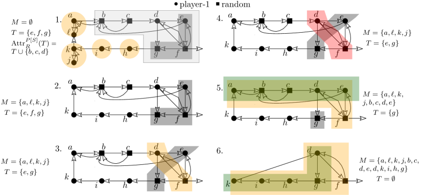
Figure 4: Example Execution of $\textsc{SymMec}(\cdot)$ on a strongly connected set of vertices with a random edge leaving it.

Figure 4 illustrates a call to SymMec with a strongly connected set of vertices $S=\{a,b,c,d,e,f,g,h,i,j,k,\ell\}$. In the first step, we compute that $\mathsf{ROut}(S)=\{f\}$ is nonempty, i.e., $S$ cannot be a MEC. We then successfully compute a separator $T$ of $S$ and recurse on the SCCs of $S\setminus\mathsf{Attr}_{R}^{P[S]}(T)=\{\{a,\ell\},\{k,j\},\{i\},\{h\}\}\}$ (orange circles). In the second step, we collapse two nontrivial MECs identified by the recursion and add them to $M$. Next, we execute the incremental EC detection for all vertices in $T$: In step three, we pick $f\in T$, remove it from $T$ and compute its SCC $S^{\prime}=\{d,f\}$ in $S\setminus T$. In step four, we compute the random attractor of $\mathsf{ROut}(S^{\prime})=\{f\}$ (in the MDP $P[S^{\prime}]$) which is equal to $S^{\prime}$ and, thus, $M$ remains unchanged. In step five, we remove $e$ from $T$ and compute its SCC $S^{\prime}=\{a,b,c,d,e,f\}$ in $S\setminus T$. In this iteration, the random attractor $Z=\{f\}$ of $\mathsf{ROut}(S^{\prime})=\{f\}$ in $P[S^{\prime}]$ is not equal to $S^{\prime}$ and we add the SCC of $e$ in $S^{\prime}\setminus Z$, i.e.,$\{a,b,c,d,e\}$ to the set of nontrivial MECs $M$ and collapse it. In step six, we analyze the SCC of the last vertex in the separator $T$, i.e., $g$ and identify an EC consisting of the vertices $\{d,g,h,i,k\}$ which we add to $M$. Since $T$ is empty $\textsc{SymMec}(S,\gamma,P)$ returns $M$.

Remark 1.

Note that our symbolic algorithm does not require randomization which is in contrast to the best known MEC decomposition algorithms for the standard RAM model [2]. The latter algorithms rely on decremental SCCs algorithms that are randomized as they maintain ES-trees [28] from randomly chosen centers. Instead, our symbolic algorithm relies on a deterministic incremental approach.

1:procedure SymMec($S,\gamma,P$)

2:     $M\leftarrow\emptyset$;

3:     if $|S|\leq 1$ then return $\emptyset$;

4:     if $\mathsf{ROut}(S)=\emptyset$ then$\triangleright$ check if $S$ is an EC

5:         $\textsc{CollapseEC}(S,P)$;

6:         return $S$;      

7:     $(T=\{v_{1},\dots,v_{t}\})\leftarrow\textsc{Separator}(S,\mathsf{Pick}(S),\gamma)$;

8:     if $T\neq\emptyset$ then $\triangleright$ $T\neq\emptyset$ if $\mathsf{diam}(S)\geq 2\gamma$

9:         $A\leftarrow\mathsf{Attr}_{R}^{P[S]}(T)$;

10:         while $S_{j}\leftarrow\mathsf{SCC\mbox{-}Find}_{P}(S\setminus A,\emptyset)$ do

11:              $M\leftarrow M\cup\textsc{SymMec}(S_{j},\gamma,P)$;          

12:         while $T\neq\emptyset$ do$\triangleright$ incremental EC detection for $v\in T$

13:              $v\leftarrow\mathsf{Pick}(T)$;

14:              $T\leftarrow T\setminus\{v\}$;

15:              $S^{\prime}\leftarrow\mathsf{SCC\mbox{-}Find}_{P}(S\setminus T,\{v\})$;

16:              if $|S^{\prime}|=1$ then continue; $\triangleright$ EC is trivial

17:              $Z\leftarrow\mathsf{Attr}_{R}^{P[S^{\prime}]}(\mathsf{ROut}(S^{\prime}))$;

18:              $S^{\prime}\leftarrow S^{\prime}\setminus Z$;

19:              if $S^{\prime}\neq\emptyset$ then$\triangleright$ $S^{\prime}$ contains a non-trivial EC

20:                  $U\leftarrow\mathsf{SCC\mbox{-}Find}_{P}(S^{\prime},\{v\})$;

21:                  $\textsc{CollapseEC}(U,P)$;

22:                  $M\leftarrow M\cup U$;                        

23:         return $M$;

24:     else$\triangleright$ $T=\emptyset$ and thus $\mathsf{diam}(S)<2\gamma$

25:         $X\leftarrow\mathsf{Attr}_{R}^{P[S]}(\mathsf{ROut}(S))$;

26:         while $S_{j}\leftarrow\mathsf{SCC\mbox{-}Find}_{P}(S\setminus X,\emptyset)$ do

27:              $M\leftarrow M\cup\textsc{SymMec}(S_{j},\gamma,P);$          

28:         return $M$;      

Figure 5: Recursively compute all vertices in nontrivial end-components in a strongly connected set of vertices.

IV-C Correctness

We prove the correctness of $\textsc{SymMec}(S,\gamma,P)$ first which will then imply the correctness of $\textsc{SymbolicMec}(P^{\prime},\gamma)$. To this end, consider an MDP $P=(V,E,\langle V_{1},V_{R}\rangle,\delta)$ and an SCC $C$ of $P$. The non-trivial end-components of a subset $S$ of $V$ are given by $\mathsf{EC}(S)$ and the set of vertices that appear in non-trivial (maximal) ECs of $C$ are denoted by $M_{C}=\bigcup_{Q\in\mathsf{EC}(C)}Q$. We observe that in all calls to $\textsc{SymMec}(S,\gamma,P)$ (see Figure 5) $S$ is strongly connected.

Lemma 6.

For a strongly connected set $S\subseteq C$ we have that in the computation of $\textsc{SymMec}(S,\gamma,P)$ for all the calls $\textsc{SymMec}(S_{j},\gamma,P)$ the set $S_{j}$ is strongly connected and $S_{j}\subseteq S$.

Proof.

If $|S|=1$ or $\mathsf{ROut}(S)=\emptyset$ there are no recursive calls and the statement is true. Now consider the case where $T\not=\emptyset$. At Line 11, we consider $S_{j}$ which is an SCC in the graph $S\setminus(T\cup A)$, obviously a subset of $S$ and strongly connected. Now consider the case where $T=\emptyset$. At Line 27 we consider $S_{j}$ which is an SCC of $S\setminus X$, obviously a subset of $S$ and strongly connected. ∎

Let $M$ be the set returned by $\textsc{SymMec}(S,\gamma,P)$. Note that the ultimate goal of $\textsc{SymMec}(S,\gamma,P)$ is to compute $M_{C}$ for a given SCC $C$ of $P^{\prime}$. The next lemma shows that every call to $\textsc{SymMec}(S,\gamma,P)$ with a strongly connected set $S$ returns a set containing $M_{S}=\bigcup_{Q\in\mathsf{EC}(S)}Q$ and collapses all ECs $Q\in\mathsf{EC}(S)$ in $P$.

Lemma 7.

Let $S$ be a strongly connected set of vertices and $M$ be the set returned by $\textsc{SymMec}(S,\gamma,P)$, then for all non-trivial ECs $Q\in\mathsf{EC}(S)$ in $P^{\prime}$ we have $Q\subseteq M$ and $Q$ is collapsed in $P$.

Proof.

Let $Q\in\mathsf{EC}(C)$ with $Q\subseteq S$. We prove the statement by induction on the size of $S$. For the base case, i.e., if $S$ is empty or contains only one vertex, $\textsc{SymMec}(S,\gamma,P)$ returns the empty set at Line 3 and thus the condition holds.

For the inductive step, let $|S|>1$. If $Q=S$, we detect it at Line 4 and return $S$ at Line 6. Then we collapse the set of vertices at Line 5. Thus, $M$ contains $Q$ and the claim holds. We distinguish two cases concerning $T$ at Line 7: First, if $T$ is non-empty then the random attractor $A$ of $T$ at Line 9 is non-empty. Thus the SCCs of $S\setminus A$ are strictly smaller than $S$. Thus, we can use the induction hypothesis to stipulate that if $Q$ is contained in one of the SCCs computed at Line 10 we have $Q\subseteq M$ after the while-loop at Lines 10-11. Additionally, by the induction hypothesis, they are collapsed. Also, if $Q$ contains a subset $Q^{\prime}\subset Q$ that is a non-trivial EC and contained in one of the SCCs of $S\setminus A$, we have that $Q^{\prime}\subseteq M$ after the while-loop at Lines 10-11. Again, by induction hypothesis, $Q^{\prime}$ is collapsed. We proceed by proving that the separator $T$ must contain one of the vertices of $Q$.

Claim 1.

For any non-trivial EC $Q\in\mathsf{EC}(S)$ which is not fully contained in one of the SCCs computed at Line 10 we have $T\cap Q\not=\emptyset$.

Proof.

Let $Q$ be an arbitrary EC in $\mathsf{EC}(S)$. Observe that if $Q$ is not fully contained in an SCC of $S\setminus A$ (computed at Line 10), we have $Q\cap A\neq\emptyset$. We now show that $Q\cap T\neq\emptyset$: Assume the contrary, i.e., $Q\cap T=\emptyset$. Consequently, $Q$ is a strongly connected set in $S\setminus T$ and not fully contained in an SCC of $S\setminus A$. Also, $Q$ contains a vertex of $A\setminus T$. Let $v\in Q\cap(A\setminus T)$ such that there is no $v^{\prime}\in Q\cap(A\setminus T)$ which is on a lower level of the attractor $A$. If $v\in V_{1}$, by the definition of the attractor and the above assumption, all its outgoing edges leave the set $Q$, which is in contradiction to $Q$ being strongly connected. Thus we have $v\in V_{R}$ and, by the definition of the attractor, $v$ must have an edge to a smaller level and by the above assumption the vertex in the smaller level is not in $Q$. That is, $Q$ has an outgoing random edge which contradicts the assumption that $Q$ is an EC. ∎

The following claim shows an invariant for the while-loop at Line 12.

Claim 2.

For iteration $j\geq 0$ of the while-loop at Line 12 holds: (a) There are no non-trivial ECs $Q\subseteq S\setminus T$ in $P$ and (b) in each iteration $j$ every nontrivial maximal EC in $S\setminus T$ is collapsed and added to $M$.

Proof.

The induction base $j=0$ holds for the following reasons: $A\setminus T$ cannot include $Q$ due to Claim 1. $S\setminus A$ cannot contain $Q$ due to the fact that $Q$ must contain a vertex in $T$ and that we collapsed the ECs contained in SCCs computed at Line 10. For the induction step, assume that there are no non-trivial ECs in $S\setminus T$ before iteration $j=\ell$. When we include one vertex $v$ of $T$ into $S$ at Line 13 there can only be one new non-trivial maximal EC $Q_{v}$ in $S$, i.e., the one including $v$, as the remaining graph is unchanged. We argue that if such an EC $Q_{v}$ exists it is collapsed into a vertex and added into $M$ before iteration $\ell+1$ of the while-loop at Line 12: The EC $Q_{v}$ must be strongly connected, and thus it is contained in the SCC $S^{\prime}$ of $v$ at Line 15. Note, that if $|S^{\prime}|=1$, the new EC is trivial, which concludes the proof. Otherwise, we compute $Z$ at Line 17, which does not contain a vertex of $Q_{v}$ by Lemma 2 and remove it from $S^{\prime}$. If $S^{\prime}$ is non-empty, it contains exactly one maximal EC as we argued above. That is the EC $Q_{v}$ and we thus add $Q_{v}$ to $M$ and collapse it. As a consequence there is no non-trivial EC in $S\setminus T$ left. Thus the claim holds. ∎

We show that $\textsc{SymMec}(S,\gamma,P)$ detects $Q$ if it is not fully contained in one of the SCCs computated at Line 10. By Claim 1 and because we iteratively remove vertices from $T$ (Lines 13–14) there exists an iteration of the while loop at Line 12 such that $Q\subseteq S\setminus T$ holds at Line 14. We show that $Q$ is in $M$ after this iteration: Because $Q$ might contain non-trivial ECs $Q^{\prime}_{i}$ that were already collapsed due to the recursive call at Line 11, or in a prior iteration of the while-loop at Line 12, it follows from Lemma 5(b) that there exists an EC $Q^{\prime}\subseteq Q$ in $P$ such that $Q^{\prime}\supseteq(Q\setminus M)$ and $Q^{\prime}$ contains one vertex corresponding to each collapsed sub-ECs $Q^{\prime}_{i}$. Due to Claim 2 we collapse $Q^{\prime}$ in the current iteration and add $Q^{\prime}$ to $M$. It follows that $Q\subseteq M$ and that $Q$ is collapsed.

Now consider the case $T=\emptyset$ (i.e., $\mathsf{diam}(S)<2\gamma$). As $\mathsf{ROut}(S)\not=\emptyset$ we have that the set $X$ computed at Line 25 is non-empty. Note that $Q$ cannot contain a vertex in $X$ by Lemma 2 and the fact that $S$ is strongly connected by Lemma 6. Consequently, $Q$ is contained in one of the SCCs of $S\setminus X$. Note that each such SCC has size strictly smaller than $S$ due to the fact that $X$ is non-empty. The claim then holds by the induction hypothesis. This completes the proof of Lemma 7. ∎

By the above lemma, we have that the algorithm finds all ECs. We next show that all vertices added to $M$ are actually contained in some EC.

Lemma 8.

The set $M$ is a subset of $M_{S}$, i.e., $M\subseteq\bigcup_{Q\in\mathsf{EC}(S)}Q$.

Proof.

We show the claim by induction over the size of $S$. For the base case, i.e., $|S|\leq 1$ the claim holds trivially because we return the empty set at Line 3 and any set of size less than two only contains trivial ECs. For the inductive step, let $|S|>1$. For the return statement at Line 6 we argue as follows: Because $S$ has no random vertices with edges out of $S$ (considering $P^{\prime}$, Line 4), $S$ is a non-trivial EC. Thus, in Line 6 we correctly return $S$.

For the case $T\not=\emptyset$ we argue as follows: Let $T$, $A$ be the separator and its attractor as computed in Line 7 and Line 9. Note that for all SCCs $S_{j}$ in the graph $S\setminus A$ we have $|S_{j}|<|S|$ because $|A|>0$. Thus, by induction hypothesis, all vertices added in the recursive call at Line 11 are in $M_{S}$. We claim that for each iteration of the while loop in Line 12 we add only non-trivial ECs to $M$: Let $v$ be the vertex we choose to remove from $T$ at Line 13. Let $S_{v}$ be the SCC of $v$ computed at Line 15. If $|S_{v}|=1$ we continue to the next iteration without adding anything to $M$ and the claim holds. Otherwise, there are two cases based on the computation of the attractor $Z$ of random vertices with edges out of $S_{v}$ at Line 17: If $Z$ contains $S_{v}$, we do not add vertices to $M$ and the claim holds. If $S_{v}\setminus Z\neq\emptyset$ we add the SCC $S^{\prime}_{v}$ of $v$ in $S_{v}\setminus Z$ to $M$. It remains to show that the non-trivial SCC $S^{\prime}_{v}$ as computed at Line 18 is a non-trivial EC:

Recall that by Claim 2 a maximal non-trivial EC within the SCC $S^{\prime}$ at Line 15 has to contain $v$. When we remove the random attractor $Z$ of $\mathsf{ROut}(S^{\prime})$ then we either end up with the empty set or with a set $S^{\prime}\leftarrow S^{\prime}\setminus Z$ that has some non-trivial SCCs with no random outgoing edges. Note that for $u\in S^{\prime}_{v}\cap V_{1}$ we have $\mathit{Out}(u)\cap S^{\prime}_{v}\neq\emptyset$ (otherwise $u\in Z$) and for $u\in S^{\prime}_{v}\cap V_{R}$ we must have $\mathit{Out}(u)\subseteq S^{\prime}_{v}$ (otherwise $u\in Z$). These bottom SCCs are also ECs and, by the above, contain $v$. Thus there is a unique maximal bottom SCC and Line 20 returns that bottom SCC.

Note that for all $v\in S^{\prime}_{v}\cap V_{1}$ we have $\mathit{Out}(v)\cap S^{\prime}_{v}\neq\emptyset$, otherwise $v\in Z$. Also, for all $u\in S^{\prime}_{v}\cap V_{R}$ we must have $\mathit{Out}(u)\subseteq S^{\prime}_{v}$, otherwise $u\in Z$. Thus, $|S^{\prime}_{v}|>1$ and all random edges again go to $S^{\prime}_{v}$.

For the case $T=\emptyset$ note that each SCC found at Line 26 are of size strictly less than $|S|$ because $|X|\geq 1$. Thus, by induction hypothesis, the vertices added at Line 27 are in $M_{S}$. ∎

Lemma 7 and Lemma 8 imply the correctness of $\textsc{SymMec}(S,\gamma,P)$ and $\textsc{SymbolicMec}(P^{\prime},\gamma)$.

Proposition 1 (Correctness).

Given an SCC $S$ of an MDP, $\textsc{SymMec}(S,\gamma,P)$ returns the set $M_{S}=\bigcup_{Q\in\mathsf{EC}(S)}Q$, i.e., the set of vertices that are contained in a non-trivial MEC of $S$.

Proposition 2 (Correctness).

$\textsc{SymbolicMec}(P^{\prime},\gamma)$ returns the set of non-trivial MECs of an MDP $P^{\prime}$.

Proof.

Due to Proposition 1 $M$ contains all vertices in nontrivial ECs. It remains to show that the nontrivial MECs are the SCCs of $M$. By definition, each nontrivial EC is strongly connected. Towards a contradiction assume that a nontrivial MEC $Q$ is not an SCC by itself but part of some larger SCC $C$ of $M$. But then, because $M$ contains only vertices in nontrivial ECs, we have that $C$ is the union of several ECs, i.e., it is strongly connected and has no random outgoing edges and thus $C$ is an $EC$. This is in contradiction to $Q$ being a MEC. Thus, each nontrivial MEC is an SCC and because $M$ contains only vertices in nontrivial ECs the union of the MECs covers $M$. Thus there are no further SCCs. ∎

IV-D Symbolic Operations Analysis

We first bound the total number of symbolic operations for computing the separator $T$ at Line 7, recursing upon the SCCs $S\setminus T$ at Line 11 and adding the vertices in $T$ back to compute the rest of the ECs of $S$ at Lines 12–23 during all calls to $\textsc{SymMec}(S,\gamma,P)$.

Lemma 9.

The total number of symbolic operations of Lines 7–23 in all calls to $\textsc{SymMec}(S,\gamma,P)$ is in $O\left(\frac{n^{2}}{\lfloor\gamma/(2\log n)\rfloor}\right)$.

Proof.

In Lemma 4 we proved that computing the separator at Line 7 takes $O(|S|)$ symbolic operations. The same holds for computing the attractor at Line 9 due to Lemma 1 and computing the SCCs at Line 10. Each iteration of the while-loop at Line 12 takes $O(|S|)$ symbolic operations: Computing the SCC of $v$ twice can be done in $O(|S|)$ symbolic operations due to Theorem 1. Similarly, computing the random attractor at Line 17 is in $O(|S|)$ symbolic operations due to Lemma 1. The remaining lines can be done in a constant amount of symbolic operations. It remains to bound the symbolic operations of the while-loop at Line 10 where we call $\textsc{SymMec}(S_{j},\gamma,P)$ recursively at Line 11 for each SCC $S_{j}$ in $S\setminus A$. Note that the size of $T$ determines the number of iterations the while-loop at Line 12 has, and how big the SCCs in $S\setminus A$ are. We obtain that $|T|$ is of size at most $\frac{|S|}{\lfloor\gamma/(2\log|S|)\rfloor}$ combining Observation 1 and Lemma 3. Due to the argument above the following equation bounds the running time of Lines 7–23 for some constant $c$ which is greater than the number of constant symbolic operations in $\textsc{SymMec}(C,\gamma,P)$ if $|S|\geq\gamma$.

$$F(S)\leq|T|\cdot|S|\cdot c+\sum_{S_{i}\in\mathsf{SCC}(S\setminus T)}F(S_{i})$$

If $|S|<\gamma$ we only have the costs for computing the separator, i.e., $F(S)\leq c\cdot|S|$. Next, we prove the bound in Claim 3.

Claim 3.

$F(S)\in O\left(\frac{|S|^{2}}{\lfloor\gamma/(2\log{|S|})\rfloor}+|S|\right)$.

Proof.

We prove the inequality m by induction on the size of $S$. That is we show $F(S)\leq\frac{|S|^{2}}{Z}c^{\prime}$ where $Z=\lfloor\gamma/(2\log|S|)\rfloor$ for some $c^{\prime}>c$. Obviously the inequality is true for $|S|<\gamma$, i.e., the base case is true. For the inductive step, consider $F(S)\leq\frac{|S|^{2}}{Z}c^{\prime}$ for $|S|\geq\gamma$. Note that

$$\sum_{S_{i}\in\mathsf{SCC}(S\setminus T)}F(S_{i}) \leq\sum_{S_{i}\in\mathsf{SCC}(S\setminus T)}c^{\prime}\frac{|S_{i}|^{2}}{\lfloor\gamma/(2\log|S_{i}|)\rfloor}+|S_{i}|\leq c^{\prime}|S|+\sum_{S_{i}\in\mathsf{SCC}(S\setminus T)}c^{\prime}|S_{i}|^{2}/Z$$

$$\leq c^{\prime}|S|+\sum_{S_{i}\in\mathsf{SCC}(S\setminus T)}c^{\prime}|S_{i}|\cdot(|S|-|T|Z)/Z\leq c^{\prime}|S|+c^{\prime}(|S|-|T|)(|S|-|T|Z)/Z$$

The first inequality is due to the induction hypothesis and the third inequality is due to the fact that we have a $Z$-separator and Lemma 3. It remains to add $|S||T|c$:

$$F(S) \leq c^{\prime}|S|+c^{\prime}(|S|-|T|)(|S|-|T|Z)/Z+|S||T|c\leq c^{\prime}|S|+\frac{c^{\prime}}{Z}(|S|^{2}-|S||T|-|T||S|Z+|T||S|)+|S||T|c$$

$$=c^{\prime}|S|+|S|^{2}/Zc^{\prime}-|S||T|c^{\prime}+|S||T|c\leq c^{\prime}|S|+\frac{|S|^{2}}{Z}c^{\prime}.$$

The first inequality is due to the fact that $|T|\leq|S|/Z$ (Observation 1). This concludes our proof by induction of $F(S)\leq c^{\prime}\cdot(\frac{|S|^{2}}{Z}+|S|)$. ∎

Using this upper bound and $|S|\leq n$ we obtain a $O\left(n^{2}/\lfloor\gamma/(2\log{n})\rfloor+n\right)$ bound which can be simplified to $O\left(n^{2}/\lfloor\gamma/(2\log{n})\rfloor\right)$ as $\gamma\leq n$. ∎

The second part of our analysis bounds the symbolic operations of the case when $\mathsf{diam}(S)<2\gamma$ at Lines 25–27 and the work done from Line 2 to Line 6.

Lemma 10.

The total number of symbolic operations of Lines 25–27 in all calls to $\textsc{SymMec}(S,\gamma,P)$ is in $O(n\cdot\gamma+\frac{n^{2}}{\lfloor\gamma/(2\log n)\rfloor})$.

Proof.

If a vertex is in the set $X$ at Line 25 it is not recursed upon or ever looked at again, thus we charge the symbolic operations of all attractor computations to the vertices in the attractor. This adds up to a total of $O(n)$ symbolic operations by Lemma 1. Additionally, note that $|X|$ is non-empty, as otherwise $|S|$ is declared as EC in the if-condition at Line 4. Thus, Lines 25–27 occur at most $n$ times. The number of symbolic operations for computing SCCs is in time $O(\sum_{C\in\mathsf{SCC}(G)}(D_{C}+1))$ due to Theorem 1. We can distribute the costs to the SCCs according to the diameters of the SCCs. We provide separate arguments for counting the costs for SCCs $S_{j}$ with $\mathsf{diam}(S_{j})<2\gamma$ and SCCs $S_{j}$ with $\mathsf{diam}(S_{j})\geq 2\gamma$. First, we consider the costs for SCCs $S_{j}$ with $\mathsf{diam}(S_{j})<2\gamma$. Computing the SCC $S_{j}$ costs $O(\gamma)$ operations and the algorithm either terminates in the next step or at least one vertex is removed from the SCC via a separator or attractor. That is we have at most $n$ such SCCs computations and thus an overall cost of $O(n\gamma)$. Now we consider the costs for SCCs $S_{j}$ with $\mathsf{diam}(S_{j})\geq 2\gamma$. Whenever computing such an SCC, we simply charge all its vertices for the costs of computing the SCC, i.e., $O(1)$ for each vertex. For such an SCC the algorithm either terminates in the next step or a separator is computed and removed. We thus have that each vertex is charged again after at least $\lfloor\gamma/(2\log|S|)\rfloor$ many nodes are removed from its SCC. In total, each vertex is charged at most $\frac{|S|}{\lfloor\gamma/(2\log|S|)\rfloor}$ many times. We get an $O(|S|\frac{|S|}{\lfloor\gamma/(2\log|S|)\rfloor})$ upper bound for the SCCs with large diameter, ∎

Putting Lemma 9 and Lemma 10 together, we obtain the $O(n\cdot\gamma+\frac{n^{2}}{\lfloor\gamma/(2\log n)\rfloor})$ bound for $\textsc{SymMec}(S,\gamma,P)$ which also applies to $\textsc{SymbolicMEC}(P^{\prime},\gamma)$ as the SCC-computations only require $O(n)$ operations.

Proposition 3.

$\textsc{SymMec}(S,\!\gamma,\!P)$ and $\textsc{SymbolicMEC}(P^{\prime},\!\gamma)$ both need $O(n\cdot\gamma+\frac{n^{2}}{\lfloor\gamma/(2\log n)\rfloor})$ symbolic operations.

IV-E Symbolic Space

Symbolic space usage counted as the maximum number of sets (and not their size) at any point in time is a crucial metric and limiting factor of symbolic computation in practice [21]. In this section, we consider the symbolic space usage of $\textsc{SymMec}(S,\gamma,P)$, highlight a key issue and present a solution to the issue.

Key Issue. Even though $\textsc{SymMec}(S,\gamma,P)$ beats the current best symbolic Algorithm for computing the MEC decomposition in the number of symbolic operations (current best: $O(n\sqrt{m})$, space: $O(\sqrt{n})$ [16]), without further improvements, $\textsc{SymMec}(S,\gamma,P)$ requires $O(n)$ symbolic space as we discuss in the following. First, note that each call of $\textsc{SymMec}(S,\gamma,P)$, when excluding the sets stored by recursive calls, only stores a constant number of sets and requires a logarithmic number of sets to execute $\mathsf{SCC\mbox{-}Find}(\cdot)$. That is, the recursion depth is the crucial factor here. As we show below, by the $\lfloor\gamma/(2\log n)\rfloor$-separator property, the recursion depth due to the case $T\not=\emptyset$ is $O\left(n/\lfloor\gamma/(2\log n)\rfloor\right)$. However, the case $T=\emptyset$ might lead to a recursion depth of $O(n)$ when in each iteration only a constant number of vertices is removed and the diameter of the resulting SCC is still smaller than $2\gamma$. As $\textsc{SymMec}(S,\gamma,P)$ uses a constant amount of sets for each recursive call, it uses $\widetilde{O}(n)$ space in total.

Reducing the symbolic space. We resolve the above space issue by modifying $\textsc{SymMec}(S,\gamma,P)$ for the case $T=\emptyset$ (see Figure 6. ): At the while loop at Line 26 we first consider the SCCs $S_{j}$ with less than $|S|/2$ vertices and recurse on them. If there is an SCC $S^{\prime}$ with more than $|S|/2$ vertices we process it at the end, i.e., we use one additional set to store that SCC until the SCC algorithm terminates. As now all the computations of the current call to $\textsc{SymMec}(S,\gamma,P)$ are done we can simply reuse the sets of the current calls to start the computation for $S^{\prime}$. We do so by setting $S$ to $S^{\prime}$ and continuing in the Line 1 of $\textsc{SymMec}(S,\gamma,P)$. Using that we only recurse on sets which are of size $\leq|S|/2$ and thus get a recursion depth of $O(\log n)$ for this case. Moreover, the modified algorithm has the same computation operations as the original one and thus the bounds for the number of symbolic operations apply as well.

25:else $\triangleright$ $T=\emptyset$ and thus $\mathsf{diam}(S)<2\gamma$

26:     $X\leftarrow\mathsf{Attr}_{R}^{P[S]}(\mathsf{ROut}(S))$; $S_{tmp}=\emptyset$;

27:     while $S_{j}\leftarrow\mathsf{SCC\mbox{-}Find}_{P}(S\setminus X,\emptyset)$ do

28:         if $S_{j}\geq|S|/2$ and $|S_{j}|>1$ then $S_{tmp}\leftarrow S_{j}$; continue;

29:         $M\leftarrow M\cup\textsc{SymMec}(S_{j},M,\gamma,P)$      

30:     if $S_{tmp}\neq\emptyset$ then $S\leftarrow S_{tmp}$; goto Line 3;

31:     return $M$;

Figure 6: Reducing the symbolic space of the $\textsc{Symmec}(\cdot)$ procedure

Lemma 11.

The maximum recursion depth of the modified algorithm is in $O(\frac{n}{\lfloor\gamma/(2\log n)\rfloor}+\log n)$.

Proof.

Consider the recursion occurring due to Line 11. Because $T$ is a $\lfloor\gamma/(2\log n)\rfloor$-separator, an SCC in $S\setminus T$ contains at most $n-\lfloor\gamma/(2\log n)\rfloor\cdot|T|\leq n-\lfloor\gamma/(2\log n)\rfloor$ vertices as $|T|\geq 1$. We determine how often we can remove $\lfloor\gamma/(2\log n)\rfloor$ from $n$ until there are no vertices left which gives the recursion depth $k$. It follows that $k=\frac{n}{\lfloor\gamma/(2\log n)\rfloor}$. Now consider the recursion occurring due to Line 27. In the modified version we have that $|S_{j}|<|S|/2$ and thus this kind of recursion is bounded by $O(\log n$). ∎

$\textsc{SymMec}(S,\gamma,P)$ has $O(n\gamma+n^{2}/\lfloor\gamma/(2\log n)\rfloor)$ many symbolic operations due to Lemma 9 and Lemma 10 and the number of sets is in $O(n/\lfloor\gamma/(2\log n)\rfloor+\log n)$ due to Lemma 11. In symbolic algorithms it is of particular interest to optimize symbolic space resources. Note that we obtain a space-time trade-off when setting the parameter $\gamma$ such that $(2\sqrt{n}+2)\log n\leq\gamma\leq n$.

For the symbolic space of $\textsc{SymbolicMEC}(P^{\prime},\gamma)$ notice that the SCC algorithms are in logarithmic symbolic space and the algorithm itself only needs to store the set $M$ and the current SCC. Thus, when we immediately output the computed MECs it only requires $O(\log n)$ additional space.

Theorem 2.

The MEC decomposition of an MDP can be computed in $O\left(n^{2-\epsilon}\log n\right)$ symbolic operations and with symbolic space $O\left(n^{\epsilon}\log n\right)$ for $0<\epsilon\leq 0.5$.

By setting $\epsilon=0.5$ we obtain that the MEC decomposition of an MDP can be computed in $\widetilde{O}(n\sqrt{n})$ symbolic operations and with symbolic space $\widetilde{O}(\sqrt{n})$.

V Symbolic Qualitative Analysis of Parity Objectives

In this section we present symbolic algorithms for the qualitative analysis of parity objectives. To present the algorithms we first introduce further definitions and notation related to parity objectives.

Plays and strategies

An infinite path or a play of an MDP $P$ is an infinite sequence $\omega=\langle v_{0},v_{1},\dots\rangle$ of vertices such that $(v_{k},v_{k+1})\in E$ for all $k\in\mathbb{N}$. We write $\Omega$ for the set of all plays. A strategy for player 1 is a function $\sigma:V^{*}\cdot V_{1}\rightarrow V$ that chooses the successor for all finite sequences $\vec{w}\in V^{*}\cdot V_{1}$ of vertices ending in a player-1 vertex (the sequence represents a prefix of a play). A strategy must respect the edge relation: for all $\vec{w}\in V^{*}$ and $v\in V_{1}$ we have $(v,\sigma(\vec{w}\cdot v))\in E$. Player 1 follows the strategy $\sigma$ if, in each player-1 move, given that the current history of the game is $\vec{w}\in V^{*}\cdot V_{1}$, she chooses the next vertex according to $\sigma(\vec{w})$. We denote by $\Sigma$ the set of all strategies for player 1. A memoryless player-1 strategy does not depend on the history of the play but only on the current vertex: For all $\vec{w},\vec{w^{\prime}}\in V^{*}$ and for all $v\in V_{1}$ we have $\sigma(\vec{w}\cdot v)=\sigma(\vec{w^{\prime}}\cdot v)$. A memoryless strategy can be represented as a function $\sigma:V_{1}\rightarrow V$. From now on, we consider only the class of memoryless strategies. Once a starting vertex $v\in V$ and a strategy $\sigma\in\Sigma$ is fixed, the outcome of the MDP $P$ is a random walk $\omega_{v}^{\sigma}$ for which the probabilities of events are uniquely defined. An event $\mathcal{A}\subseteq\Omega$ is a measurable set of plays. For a vertex $v\in V$ and an event $\mathcal{A}\subseteq\Omega$, we write $\Pr_{v}^{\sigma}(\mathcal{A})$ for the probability that a play belongs to $\mathcal{A}$ if the game starts from the vertex $v$ and player 1 follows the strategy $\sigma$.

Objectives

We define objectives for player 1 as a set of plays $\Phi\subseteq\Omega$. We say that a play $\omega$ satisfies the objective $\Phi$ if $\omega\in\Phi$. We consider $\omega$-regular objectives [39], specified as parity conditions and reachability objectives which are an important subset of $\omega$-regular objectives.

Reachability objectives. Given a set $T\subseteq V$ of “target” vertices, the reachability objective requires that some vertex of $T$ be visited. The set of winning plays is in $\mathrm{Reachability(T)}=\{\langle v_{0},v_{1},\dots\rangle\in\Omega\mid v_{k}\in T\text{ for some }k\geq 0\}$.

Parity objectives. A parity objective consists of a priority function which assigns an priority to each vertex, i.e, $p:V\mapsto\{0,1,\dots,2d\}$ where $d\in\mathbb{N}$. For a play $\omega=\langle v_{0},v_{1},\dots\rangle\in\Omega$, we define $\mathrm{Inf(\omega)}=\{v\in V\mid v_{k}=v\text{ for infinitely many k }\}$ to be the set of vertices that occur infinitely often in $\sigma$. The parity objective is defined as the set of plays such that the minimum priority occurring infinitely often is even, i.e., $\mathrm{Parity(p)}=\{\omega\in\Omega\mid\min_{v\in\mathrm{Inf(\omega)}}{p(v)}\text{ is even}\}$.

Qualitative analysis: almost-sure winning. Given a parity objective $\mathrm{Parity(p)}$, a strategy $\sigma\in\Sigma$ is almost-sure winning for player 1 from the vertex $v$ if $\Pr_{v}^{\sigma}(\mathrm{Parity(p)})=1$. The almost-sure winning set $\langle\!\langle 1\rangle\!\rangle_{\mathit{almost}}(\mathrm{Parity(p)})$ for player-1 is the set of vertices from which player 1 has an almost-sure winning strategy. The qualitative analysis of MDPs corresponds to the computation of the almost-sure winning set for $\mathrm{Parity(p)}$. It follows from the results of [24, 26] that for all MDPs and parity objectives, if there is an almost-sure winning strategy, then there is a memoryless almost-sure winning strategy.

Theorem 3 ([24, 26]).

For all MDPs $P$, and all parity objectives $\mathrm{Parity(p)}$, there exists a memoryless strategy $\sigma$ such that for all $v\in\langle\!\langle 1\rangle\!\rangle_{\mathit{almost}}(\mathrm{Parity(p)})$ we have $\Pr_{v}^{\sigma}(\mathrm{Parity(p)})=1$.

V-A Almost-sure Reachability.

In this section we present a symbolic algorithm which computes reachability objectives $\mathrm{Reachability(T)}$ in an MDP. The algorithm is a symbolic version of [10, Theorem 4.1].

Graph Reachability. For a graph $G=(V,E)$ and a set of vertices $S$, the set $\mathsf{GraphReach}_{G}(S)$ is the set of vertices $V$ that can reach a vertex of $S$ within $G$. We compute it by repeatedly calling $S\leftarrow\mathsf{Pre}_{E}(S)$ until we reach a fixed point. In the worst case, we add one vertex in each such call and need $|\mathsf{GraphReach}_{G}(S)\setminus S|+1=O(n)$ many $\mathsf{Pre}_{E}(\cdot)$ operations to reach a fixed point.

Algorithm Description. Given an MDP $P$ we compute the set $\langle\!\langle 1\rangle\!\rangle_{\mathit{almost}}(\mathrm{Reachability(T)})$ as follows: First, if player 1 can reach one vertex of a MEC he can reach all the vertices of a MEC and thus we can collapse each MEC $M$ to a vertex. If $M$ contains a vertex of $T$, we set $T\leftarrow T\cup M$, i.e. $T$ contains the vertex which represents $M$. $P^{\prime}=(V^{\prime},E^{\prime},\langle V^{\prime}_{1},V^{\prime}_{2}\rangle,\delta^{\prime})$ is the MDP where the MECs of $P$ are collapsed as described above. Next, we compute the set of vertices $S$ which can reach $T$ in the graph induced by $P^{\prime}$. A vertex in $V^{\prime}\setminus S$ cannot reach $T$ almost-surely because there is no path to $T$. Note that a play starting from a vertex in the random attractor $A$ of $V^{\prime}\setminus S$ might also end up in $V^{\prime}\setminus S$. We thus remove $A$ from $V^{\prime}$ to obtain the set $R$, where vertices can almost-surely reach $T$ in $P^{\prime}$. Finally, to transfer the result back to $P$ we include all MECs with a vertex in $R$.

We implement $\textsc{SymbolicMEC}(P^{\prime},\gamma)$ to compute the MEC decomposition of $P$ but note that we could use any symbolic MEC algorithm. To minimize the extra space usage we also assume that the algorithm which computes the MEC decomposition outputs one MECs after the other instead of all MECs at once. Note that we can easily modify $\textsc{SymbolicMEC}(P^{\prime},\gamma)$ to output one MEC after the other by iteratively returning each SCC found at Line 5. Moreover, we only require logarithmic space to maintain the state of the SCC algorithm [9].

1:procedure SymASReach($T,P$)

2:     $V^{\prime}\leftarrow V;E^{\prime}\leftarrow E;V^{\prime}_{1}\leftarrow V_{1};V^{\prime}_{R}\leftarrow V_{R};\delta^{\prime}\leftarrow\delta$;

3:     $P^{\prime}=(V^{\prime},E^{\prime},\langle V^{\prime}_{1},V^{\prime}_{R}\rangle,\delta^{\prime})$;

4:     for $M\leftarrow\textsc{ComputeMECs}(P)$ do

5:         $\textsc{CollapseEC}(M,P^{\prime})$;

6:         if $M\cap T\neq\emptyset$ then $T\leftarrow T\cup M$;      

7:     $S\leftarrow\mathsf{GraphReach}_{P^{\prime}}(T\cap V^{\prime})$; $A\leftarrow\mathsf{Attr}_{R}^{P^{\prime}}(V^{\prime}\setminus S)$; $R\leftarrow V^{\prime}\setminus A$;

8:     for $M\leftarrow\textsc{ComputeMECs}(P)$ do

9:         if $M\cap R\neq\emptyset$ then $R\leftarrow R\cup M$;      

10:     return $R$;

Figure 7: Computing $\langle\!\langle 1\rangle\!\rangle_{\mathit{almost}}(\mathrm{Reachability(T)})$ symbolically

We prove the following two propositions for $\textsc{SymASReach}(T,P)$. Let $P$ be an MDP, $T$ a set of vertices and $\mathbf{MEC}$ be the number of symbolic operations we need to compute the MEC decomposition. Let $\mathit{space}(\mathbf{MEC})$ denote the space of computing the MEC decomposition.

Proposition 4 (Correctness [9]).

$\textsc{SymASReach}(T,P)$ correctly computes the set $\langle\!\langle 1\rangle\!\rangle_{\mathit{almost}}(\mathrm{Reachability(T)})$.

Proposition 5 (Running time and Space).

The total number of symbolic operations of $\textsc{SymASReach}(T,P)$ is in $O(\mathbf{MEC}+n)$. $\textsc{SymASReach}(T,P)$ uses $\widetilde{O}(\mathit{space}(\mathbf{MEC}))$ symbolic space.

Proposition 5 and Proposition 4 together with Theorem 2 yield the following theorem.

Theorem 4.

The set $\langle\!\langle 1\rangle\!\rangle_{\mathit{almost}}(\mathrm{Reachability(T)})$ of an MDP can be computed with $\widetilde{O}(n^{2-\epsilon})$ many symbolic operations and $\widetilde{O}(n^{\epsilon})$ symbolic space for $0<\epsilon\leq 0.5$.

V-B Parity Objectives.

In this section we consider the qualitative analysis of MDPs with parity objectives. We present an algorithm for computing the winning region which is based on the algorithms we present in the previous sections and the algorithm presented in [13, Section 5]. The algorithm presented in [13, Section 5] draws ideas from a hierarchical clustering technique [38, 33]. Without loss of generality, we consider the parity objectives $\mathrm{Parity(p)}$ where $p:V\rightarrow\{0,1,\dots,2d\}$. In the symbolic setting, instead of $p$, we get the sets $\mathcal{P}_{\geq i}=\{v\in V\mid p(v)\geq i\}$ where $(1\leq i\leq 2d)$ as part of the input. We abbreviate the family $\{\mathcal{P}_{\geq i}\mid 1\leq i\leq 2d\}$ as $(\mathcal{P}_{\geq k})_{1\leq k\leq 2d}$. Let $\mathcal{P}_{\leq m}=V\setminus\mathcal{P}_{\geq m+1}$ and $\mathcal{P}_{m}=\mathcal{P}_{\geq m}\setminus\mathcal{P}_{\geq m+1}$. Given an MDP $P$, let $P_{i}$ denote the MDP obtained by removing $\mathsf{Attr}_{R}^{P}(\mathcal{P}_{\leq i-1})$, the set of vertices with priority less than $i$ and its random attractor. A MEC $M$ is a winning MEC in $P_{i}$ if there exists a vertex $u\in M$ such that $p(u)=i$ and $i$ is even, i.e., the smallest priority in the MEC is even. Let $\mathsf{WE}_{i}$ be the union of vertices of winning maximal end-components in $P_{i}$, and let $\mathsf{WE}=\bigcup_{0\leq i\leq 2d}\mathsf{WE}_{i}$. Lemma 12 says that computing $\langle\!\langle 1\rangle\!\rangle_{\mathit{almost}}(\mathrm{Parity(p)})$ is equivalent to computing almost-sure reachability of $\mathsf{WE}$. Intuitively, player 1 can infinitely often satisfy the parity condition after reaching an end-component which satisfies the parity condition.

Lemma 12 ([13]).

Given an MDP $P$ we have $\langle\!\langle 1\rangle\!\rangle_{\mathit{almost}}(\mathrm{Parity(p)})=\langle\!\langle 1\rangle\!\rangle_{\mathit{almost}}(\mathrm{Reachability(\mathsf{WE})})$.

We describe in Figure 8 how to compute $\mathsf{WE}$ symbolically.

V-B1 Algorithm Description.

The algorithm uses a key idea which we describe first. Recall that $P_{i}$ denotes the MDP obtained by removing $\mathsf{Attr}_{R}^{P}(\mathcal{P}_{\leq i-1})$, i.e., the set of vertices with priority less than $i$ and its random attractor.

Key Idea. If $u,v$ are in a MEC in $P_{i}$, then they are in the same MEC in $P_{i-1}$. The key idea implies that if a vertex is in a winning MEC of $P_{i}$, it is also in a winning MEC of $P_{i-1}$. Intuitively, this holds due to the following two facts: (1) Because $P_{i-1}$ contains all edges and vertices of $P_{i}$ the MECs $P_{i}$ are still strongly connected in $P_{i-1}$. (2) Because $\mathsf{Attr}_{R}^{P}(\mathcal{P}_{\leq i-1})$ makes sure that no MEC $M$ in $P_{i}$ has a random vertex with an edge leaving $P_{i}$ in $M$, the same is true for the set $M$ in $P_{i-1}$.

We next present the recursive algorithm $\textsc{WinPEC}((\mathcal{P}_{\geq k})_{1\leq k\leq 2d},i,j,P)$ which, for a MDP $P$, computes the set $\bigcup_{i\leq\ell\leq j}\mathsf{WE}_{i}$ of winning MECs for priorities between $i$ and $j$.

1. Base Case: If $j<i$, return $\emptyset$.

2. Compute $m\leftarrow\lceil(i+j)/2\rceil$.

3. Compute the MECs of $P_{m}=V\setminus\mathsf{Attr}_{R}^{P}(\mathcal{P}_{\leq m-1})$ and for each MEC $M\in P_{m}$ compute the minimal priority $min$ among all vertices in that MEC.

   • If $min$ is even then add $M$ to the set $W$ of vertices in winning MECs.

   • If $min$ is odd we recursively call $\textsc{WinPEC}((\mathcal{P}_{\geq k})_{1\leq k\leq 2d},min+1,j,P^{u})$ where $P^{u}$ is the sub-MDP containing only vertices and edges inside $M$. This call applies the key idea and refines the MECs of $P_{m}$ and computes the set $\bigcup_{min+1\leq\ell\leq j}\mathsf{WE}_{\ell}$.

4. Call $\textsc{WinPEC}((\mathcal{P}_{\geq k})_{1\leq k\leq 2d},i,m-1,P^{\ell})$ where $P^{\ell}$ is the MDP where all MECs in $P_{m}$ are collapsed into a single vertex and thus only the edges outside the MECs of $P_{m}$ are considered. This call computes the set $\bigcup_{i\leq k\leq m-1}\mathsf{WE}_{k}$.

The initial call is $\textsc{WinPEC}(\mathcal{P}_{\geq k})_{1\leq k\leq 2d},0,2d,P)$. Figure 8 illustrates the formal version of the sketched algorithm.

1:procedure WinPEC($(\mathcal{P}_{\geq k})_{1\leq k\leq 2d},i,j,P$)

2:     $W\leftarrow\emptyset$;

3:     if $j<i$ then return $W$;

4:     $m\leftarrow\lceil(i+j)/2\rceil$;

5:     $X_{m}\leftarrow\mathsf{Attr}_{R}^{P}(\mathcal{P}_{\leq m-1})$;

6:     $Z_{m}\leftarrow V\setminus X_{m}$; $E_{m}\leftarrow E\cap(Z_{m}\times Z_{m})$;

7:     $P^{\prime}\leftarrow(Z_{m},E_{m},\langle V_{1}\cap Z_{m},V_{R}\cap Z_{m}\rangle,\delta^{\prime})$;

8:     for $M\leftarrow\textsc{ComputeMECs}(P^{\prime})$ do

9:         $min\leftarrow minPriority(M)$;

10:         if $min$ is even then

11:              $W\leftarrow W\cup M$;

12:         else

13:              $V^{u}\leftarrow M\setminus\mathsf{Attr}_{R}^{P}(\mathcal{P}_{min})$;

14:              $P^{u}\leftarrow(V^{u},(V^{u}\times V^{u})\cap E,\langle V_{1}\cap V^{u},V_{R}\cap V^{u}\rangle,\delta^{u})$;

15:              $W\leftarrow W\cup\textsc{WinPEC}((\mathcal{P}_{\geq k})_{1\leq k\leq 2d},min+1,j,P^{u})$;               

16:     for $M\leftarrow\textsc{ComputeMECs}(P^{\prime})$ do

17:         $\textsc{CollapseEC}(M,P);$ $\triangleright$ MDP with MECs collapsed is $P^{\ell}$      

18:     $W\leftarrow W\cup\textsc{WinPEC}((\mathcal{P}_{\geq k})_{1\leq k\leq 2d},i,m-1,P)$;

19:     return $W$;

Figure 8: Algorithm to compute $\mathsf{WE}$ of the MDP $P$ recursively

V-B2 Correctness and Number of Symbolic Steps.

In this section we argue that $\textsc{WinPEC}(\cdot)$ is correct and bound the number of symbolic steps and the symbolic space usage. A key difference in the analysis of $\textsc{WinPEC}(\cdot)$ and [13] is that we aim for a symbolic step bound that is independent from the number of edges in $P$ and, thus, we cannot use the argument from [13] which charges the cost of each recursive call to the edges of $P$. The key argument in [13] is that the sets of edges in the different branches of the recursions do not overlap. For vertices it is not that simple, as we do not entirely remove vertices that appear in a MEC but merge the MEC and represent it by a single vertex. That is, a vertex can appear in both $P^{\ell}$ and in $P^{u}$ corresponding to the MEC. In order to accomplish our symbolic step bound we adjusted the algorithm. At Line 13 we always remove the minimum priority vertices instead of removing the vertices with priority $m$ to ensure that we remove at least one vertex. Intuitively, by always removing at least one vertex from a MEC we ensure that the total number of vertices processed at each recursion level does not grow. Note that these changes of the algorithm do not affect the correctness argument of [13] as we always compute the same sets $\mathsf{WE}_{m}$ but avoid calls to $\textsc{WinPEC}(\cdot)$ with no progress on some MECs.

Proposition 6 (Correctness).

$\textsc{WinPEC}(\cdot)$ returns the set of winning end-components $\mathsf{WE}$.

Proof.

The correctness of the algorithm is by induction on $j-i$ for the induction hypothesis $\bigcup_{i\leq\ell\leq j}\mathsf{WE}_{\ell}\subseteq\textsc{WinPEC}((\mathcal{P}_{\geq k})_{1\leq k\leq 2d},i,j,P)\subseteq\bigcup_{1\leq\ell\leq 2d}\mathsf{WE}_{\ell}$.

First consider the induction base cases: If $j>i$, the algorithm correctly returns the empty set. Next, consider the induction step. Assume that the results hold for $j-i\leq k$, and we consider $j-i=k+1$. If $m$ is even, then

$$\bigcup_{i\leq k\leq j}\mathsf{WE}_{k}=\mathsf{WE}_{m}\cup\bigcup_{i\leq k\leq m-1}\mathsf{WE}_{k}\cup\bigcup_{m+1\leq k\leq j}\mathsf{WE}_{k},$$

otherwise ($m$ is odd), then

$$\bigcup_{i\leq k\leq j}\mathsf{WE}_{k}=\bigcup_{i\leq k\leq m-1}\mathsf{WE}_{k}\cup\bigcup_{m+1\leq k\leq j}\mathsf{WE}_{k},$$

Consider an arbitrary winning MEC $M_{k}$ in $P_{k}$, i.e., the lowest even priority is $k$. We consider the following cases.

1. For all $k\geq m$ we have that $M_{k}$ is contained in a MEC $M_{m}$ of $P_{m}$. Additionally, no random vertex in $M_{m}$ can have an edge leaving $M_{m}$ and thus no random vertex in $M_{k}$ can have a random edge leaving $M_{m}$. Moreover, for the minimum priority $min$ of $M_{m}$ we have $k\geq min\geq m$. If $min$ is even then $M_{m}$ is itself winning and thus $M_{k}\subseteq\textsc{WinPEC}((\mathcal{P}_{\geq k})_{1\leq k\leq 2d},i,j,P)$ and $M_{m}\subseteq\bigcup_{1\leq\ell\leq 2d}\mathsf{WE}_{\ell}$ (note that it might be that $min>j$).

   If $min$ is odd we have that $M_{k}$ is a winning MEC of $P$ iff it is a winning MEC of $P^{u}$ and thus by the induction hypothesis $M_{k}\subseteq\textsc{WinPEC}((\mathcal{P}_{\geq k})_{1\leq k\leq 2d},min+1,j,P^{u})$. It follows that also $M_{k}\subseteq\textsc{WinPEC}((\mathcal{P}_{\geq k})_{1\leq k\leq 2d},i,j,P)$.

2. For $k<m$ consider a MEC $M_{k}$ in $P_{k}$. If $M_{k}$ contains a vertex $v$ that belongs to a MEC $M_{m}$ of $P_{m}$, then $M_{m}\subset M_{k}$ (i.e., all vertices of the MEC in $P_{m}$ of $v$ also belong to $M_{k}$ and $M_{k}$ has at least one additional vertex with priority $<m$). We thus have that for $k\leq m$ the winning MECs $M_{k}$ in $P_{k}$ are in one-to-one correspondence with the winning MECs $M^{\prime}_{k}$ of the modified MDP where all MECs of $P_{m}$ are collapsed. From the induction hypothesis it follows that $\bigcup_{i\leq k\leq m-1}\mathsf{WE}_{k}=\textsc{WinPEC}((\mathcal{P}_{\geq k})_{1\leq k\leq 2d},i,m-1,P)$

Hence we have that $\bigcup_{i\leq k\leq j}\mathsf{WE}_{k}\subseteq\textsc{WinPEC}((\mathcal{P}_{\geq k})_{1\leq k\leq 2d},i,j,P)\subseteq\bigcup_{1\leq\ell\leq 2d}\mathsf{WE}_{\ell}$. The statements follows from setting $i=0$ and $j=2d$. ∎

Proposition 7 (Symbolic Steps).

The total number of symbolic operations for $\textsc{WinPEC}(\cdot)$ is $O(\mathbf{MEC}\cdot\log d)$ for $0<\epsilon\leq 0.5$.

Proof.

Given an MDP $P$ with $n$ vertices and $d$ priorities, let us denote by $T(n,x)$ the number of symbolic steps of $\textsc{WinPEC}(\cdot)$ at recursion depth $x$ and with $T_{M}(n)$ the number of symbolic steps incurred by the symbolic MEC Algorithm. As shown in [13], note that the recursion depth of $\textsc{WinPEC}(\cdot)$ is in $O(\log d)$ because we recursively consider either $(min+1,j)$ or $(i,m-1)$ where $min\geq m=\lceil(i+j/2)\rceil$ until $j>i$, where $j=2d$ initially. First, we argue that there exists $c>0$ such that $T(n,x)\leq c\cdot T_{M}(n)+(\sum_{i=1,\dots,t}T\left(n_{i},x-1\right))\\ +T(n-(\sum_{i=1,\dots,t}n_{i})+t,x-1)\text{ if }x>1$ and $T(n,0)\leq c.$ The attractors computed at Line 5 and Line 13 can be done in $O(n)$ symbolic steps as the set of vertices in the attractors are all disjunct. Clearly, this is cheaper than computing the MEC decomposition. To extract the minimum priority of a set of nodes $X\subseteq V$ we apply a binary search procedure which takes $O(\log d)$ symbolic steps at Line 9. Note that when $\log d>n$ we cannot charge the cost to computing the MEC decomposition. Thus, we argue in Claim 4 that the total number of symbolic steps for Line 9 in $\textsc{WinPEC}(\cdot)$ is less than $O(n\log d)$. The rest of the symbolic steps in $\textsc{WinPEC}(\cdot)$, (except the recursive calls and computing the MEC decomposition) in $\textsc{WinPEC}(\cdot)$ can be done in a constant amount of symbolic steps. Note that when $x=0$, i.e., in the case $j<i$, we only need a constant amount of symbolic steps. Let $t$ be the number of MECS in $P^{\prime}$. When $x>0$, consider the following argumentation for the number of symbolic steps of the recursive calls:

• $\textsc{WinPEC}((\mathcal{P}_{\geq k})_{1\leq k\leq 2d},min,j,P^{u})$: We perform the recursive call for each MEC $M_{i}\in P^{\prime}$ $(1\leq i\leq t)$ where the vertex with minimum priority is odd. The total cost incurred by all such recursive calls is $\sum_{i=1,\dots,t}T(n_{i},x-1)$ where $n_{i}\leq|M_{i}|-1$ because we always remove the vertices with minimum priority at Line 13.

• $\textsc{WinPEC}((\mathcal{P}_{\geq k})_{1\leq k\leq 2d},i,m-1,P^{\ell})$: $P^{\ell}$ consists of the vertices representing the collapsed MECs, the vertices not in $P^{\prime}$ and the vertices which are not in a MEC of $P^{\prime}$. The number of vertices in $P^{\ell}$ is thus $n_{\ell}=n-\sum_{i=1,\dots,t}|M_{i}|+t$ and we obtain $T(n_{\ell},x-1)$.

Note that $\sum_{i=1,\dots,t}n_{i}+n_{\ell}\leq n$. We choose $c$ such that $cT_{M}(n)$ is greater than the number of symbolic steps for computing the MECs twice and the rest of the work in the current iteration of $\textsc{WinPEC}(\cdot)$. It is straightforward to show that $T(n,d)=O(T_{M}(n)\log d)$.

The following claim shows that the total number of symbolic steps incurred by Line 9 for all calls to $\textsc{WinPEC}(\cdot)$ is only $O(n\log d)$.

Claim 4.

The total amount of symbolic steps used by Line 9 is in $O(n\log d)$.

Proof.

To obtain the set of vertices with minimum priority from a set of vertices $X\subseteq V$ the function $\mathsf{MinPriority}_{(}X)$ performs a binary search using the sets $(\mathcal{P}_{\geq k})_{1\leq k\leq 2d}$. This can be done in $O(\log d)$ many symbolic steps. To prove that the number of symbolic steps used by Line 9 in total is in $O(n\log d)$ note that each time the function is performed we either: (i) Remove all vertices in $M$, and we never perform the function on the vertices in $M$ again. We charge the cost to an arbitrary vertex in $M$. (ii) Remove at least one vertex at Line 13 and we never perform the function on a MEC containing this vertex again. We charge the cost to this vertex. As there are only $n$ vertices we obtain that the total amount of symbolic steps used by Line 9 is in $O(n\log d)$. ∎

The symb. bound of $\textsc{WinPEC}(\cdot)$ follows by Claim 4. ∎

Proposition 8.

$\textsc{WinPEC}(\cdot)$ uses $O(\mathit{space}(\mathbf{MEC})+\log n\log d)$ space.

Proof.

Let $P$ be an MDP with $n$ vertices and $p$ a parity objective with $d$ priorities. We denote with $\mathit{space}(\mathbf{MEC})$ the symbolic space used by the algorithm that computes the MEC decomposition. Observe that all computation steps in $\textsc{WinPEC}(\cdot)$ need constant space except for the recursions and computing the MEC decomposition. Both at Line 8 and Line 16 we first compute the MEC decomposition and then, to minimize extra space, we output one MEC after the other by returning each SCC found given the set of vertices in nontrivial MECs. Note that we only require logarithmic space to maintain the state of the SCC algorithm [9]. As argued in [13] the recursion depth of $\textsc{WinPEC}(\cdot)$ is $O(\log d)$. Thus, we need $O(\log n\log d)$ space for maintaining the state of the SCC algorithm at Line 5 until we reach a leaf of the recursion tree. At each recursive call, we need additive $O(\mathit{space}(\mathbf{MEC}))$ space to compute the MEC decomposition of $P$. The claimed space bound follows. ∎

Given an MDP, we first compute the set $\mathsf{WE}$ with $\textsc{WinPEC}(\cdot)$ which is correct due to Proposition 6. We instantiate $\mathbf{MEC}$ and $\mathit{space}(\mathbf{MEC})$ in Proposition 7 and Proposition 8 respectively with Theorem 2 and thus need $O(n^{2-\epsilon}\log n\log d)$ symbolic steps and $O(n^{\epsilon}\log n+\log n\log d)$ (where $0<\epsilon\leq 0.5$) symbolic space for computing $\mathsf{WE}$. Then, we compute almost-sure reachability of $\mathsf{WE}$ with Theorem 4. Finally, using Lemma 12 we obtain the following theorem.

Theorem 5.

The set $\langle\!\langle 1\rangle\!\rangle_{\mathit{almost}}(\mathrm{Parity(p)})$ of an MDP $P$ can be computed with $\widetilde{O}(n^{2-\epsilon})$ many symbolic operations and $\widetilde{O}(n^{\epsilon})$ symbolic space for $0<\epsilon\leq 0.5$.

VI Conclusion

We present a faster symbolic algorithm for the MEC decomposition and we improve the fastest symbolic algorithm for verifying MDPs with $\omega$-regular properties. There are several interesting directions for future work. On the practical side, implementations and experiments with case studies is an interesting direction. On the theoretical side, improving upon the $\widetilde{O}(n^{1.5})$ bound for MECs is an interesting open question which would also, using our work, improve the presented algorithm for verifying $\omega$-regular properties of MDPs.

References

- [1] C. Baier and J. Katoen. Principles of model checking. MIT Press, 2008.
- [2] A. Bernstein, M. Probst, and C. Wulff-Nilsen. Decremental strongly-connected components and single-source reachability in near-linear time. In STOC, pages 365–376, 2019.
- [3] T. Brázdil, V. Brozek, K. Chatterjee, V. Forejt, and A. Kucera. Two views on multiple mean-payoff objectives in Markov decision processes. In LICS 2011, pages 33–42, 2011.
- [4] A. Browne, E. M. Clarke, S. Jha, D. E. Long, and W. R. Marrero. An improved algorithm for the evaluation of fixpoint expressions. Theoretical Computer Science, 178(1-2):237–255, 1997.
- [5] R. E. Bryant. Graph-based algorithms for boolean function manipulation. IEEE Transactions on Computers, 100(8):677–691, 1986.
- [6] R. E. Bryant. Symbolic boolean manipulation with ordered binary-decision diagrams. ACM Comput. Surv., 24(3):293–318, Sept. 1992.
- [7] J. R. Burch, E. M. Clarke, K. L. McMillan, D. L. Dill, and L. J. Hwang. Symbolic model checking: 10^20 states and beyond. In LICS, pages 428–439, 1990.
- [8] K. Chatterjee. Stochastic -Regular Games. PhD thesis, UC Berkeley, 2007.
- [9] K. Chatterjee, W. Dvořák, M. Henzinger, and V. Loitzenbauer. Lower bounds for symbolic computation on graphs: Strongly connected components, liveness, safety, and diameter. In SODA, pages 2341–2356, 2018.
- [10] K. Chatterjee, W. Dvořák, M. Henzinger, and V. Loitzenbauer. Model and objective separation with conditional lower bounds: Disjunction is harder than conjunction. In LICS, pages 197–206, 2016.
- [11] K. Chatterjee, W. Dvořák, M. Henzinger, and V. Loitzenbauer. Improved set-based symbolic algorithms for parity games. In CSL, pages 18:1–18:21, 2017.
- [12] K. Chatterjee, W. Dvořák, M. Henzinger, and A. Svozil. Near-linear time algorithms for streett objectives in graphs and MDPs. In CONCUR, pages 7:1–7:16, 2019.
- [13] K. Chatterjee and M. Henzinger. Faster and dynamic algorithms for maximal end-component decomposition and related graph problems in probabilistic verification. In SODA, pages 1318–1336, 2011.
- [14] K. Chatterjee and M. Henzinger. Efficient and dynamic algorithms for alternating Büchi games and maximal end-component decomposition. J. ACM, 61(3):15:1–15:40, 2014.
- [15] K. Chatterjee, M. Henzinger, M. Joglekar, and N. Shah. Symbolic algorithms for qualitative analysis of Markov decision processes with Büchi objectives. Form. Methods Syst. Des., 42(3):301–327, 2013.
- [16] K. Chatterjee, M. Henzinger, V. Loitzenbauer, S. Oraee, and V. Toman. Symbolic algorithms for graphs and Markov decision processes with fairness objectives. In CAV, pages 178–197, 2018.
- [17] K. Chatterjee and T. A. Henzinger. Probabilistic systems with limsup and liminf objectives. In ILC, pages 32–45, 2007.
- [18] K. Chatterjee, T. A. Henzinger, B. Jobstmann, and R. Singh. Measuring and synthesizing systems in probabilistic environments. J. ACM, 62(1):9:1–9:34, 2015.
- [19] S. Chechik, T. D. Hansen, G. F. Italiano, J. Lacki, and N. Parotsidis. Decremental single-source reachability and strongly connected components in total update time. In FOCS, pages 315–324, 2016.
- [20] E. Clarke, O. Grumberg, S. Jha, Y. Lu, and H. Veith. Counterexample-guided abstraction refinement for symbolic model checking. J. ACM, 50(5):752–794, 2003.
- [21] E. Clarke, O. Grumberg, and D. Peled. Symbolic model checking. In Model Checking. MIT Press, 1999.
- [22] E. M. Clarke, K. L. McMillan, S. V. A. Campos, and V. Hartonas-Garmhausen. Symbolic model checking. In CAV, pages 419–427, 1996.
- [23] C. Courcoubetis and M. Yannakakis. Markov decision processes and regular events. In ICALP, pages 336–349, 1990.
- [24] C. Courcoubetis and M. Yannakakis. The complexity of probabilistic verification. J. ACM, 42(4):857–907, 1995.
- [25] P. Daca, T. A. Henzinger, J. Kretínský, and T. Petrov. Faster statistical model checking for unbounded temporal properties. ACM Trans. Comput. Log., 18(2):12:1–12:25, 2017.
- [26] L. de Alfaro. Formal Verification of Probabilistic Systems. PhD thesis, Stanford University, 1997.
- [27] C. Dehnert, S. Junges, J. Katoen, and M. Volk. A Storm is coming: A modern probabilistic model checker. In CAV, pages 592–600, 2017.
- [28] S. Even and Y. Shiloach. An On-Line Edge-Deletion Problem. J. ACM, 28(1):1–4, 1981.
- [29] J. Filar and K. Vrieze. Competitive Markov Decision Processes. Springer-Verlag, 1997.
- [30] R. Gentilini, C. Piazza, and A. Policriti. Computing strongly connected components in a linear number of symbolic steps. In SODA, pages 573–582, 2003.
- [31] R. Gentilini, C. Piazza, and A. Policriti. Symbolic graphs: Linear solutions to connectivity related problems. Algorithmica, 50(1):120–158, 2008.
- [32] H. Howard. Dynamic Programming and Markov Processes. MIT Press, 1960.
- [33] V. King, O. Kupferman, and M. Y. Vardi. On the complexity of parity word automata. In FOSSACS, volume 2030 of Lecture Notes in Computer Science, pages 276–286. Springer, 2001.
- [34] J. Kretínský, G. A. Pérez, and J. Raskin. Learning-based mean-payoff optimization in an unknown MDP under omega-regular constraints. In CONCUR, pages 8:1–8:18, 2018.
- [35] M. Z. Kwiatkowska, G. Norman, and D. Parker. PRISM 4.0: Verification of probabilistic real-time systems. In CAV, pages 585–591, 2011.
- [36] M. Puterman. Markov Decision Processes. John Wiley and Sons, 1994.
- [37] F. Somenzi. Binary Decision Diagrams. In Calculational System Design, pages 303–366. IOS Press, 1999.
- [38] R. E. Tarjan. A hierarchical clustering algorithm using strong components. Inf. Process. Lett., 14(1):26–29, 1982.
- [39] W. Thomas. Languages, automata, and logic. In Handbook of Formal Languages: Volume 3 Beyond Words, pages 389–455. Springer, 1997.