Spectral transfer and Kármán-Howarth-Monin equations for compressible Hall magnetohydrodynamics

Abstract

We derive two new forms of the Kármán-Howarth-Monin equation for decaying compressible Hall magnetohydrodynamic (MHD) turbulence. We test them on results of a weakly-compressible, two-dimensional, moderate-Reynolds-number Hall MHD simulation and compare them with an isotropic spectral transfer (ST) equation. The KHM and ST equations are automatically satisfied during the whole simulation owing to the periodic boundary conditions and have complementary cumulative behavior. They are used here to analyze the onset of turbulence and its properties when it is fully developed. These approaches give equivalent results characterizing: the decay of the kinetic + magnetic energy at large scales, the MHD and Hall cross-scale energy transfer/cascade, the pressure dilatation, and the dissipation. The Hall cascade appears when the MHD one brings the energy close to the ion inertial range and is related to the formation of reconnecting current sheets. At later times, the pressure-dilation energy-exchange rate oscillates around zero with no net effect on the cross-scale energy transfer when averaged over a period of its oscillations. A reduced one-dimensional analysis suggests that all three methods may be useful to estimate the energy cascade rate from in situ observations.

1. Introduction

Turbulence is ubiquitous in astrophysical plasma environments (Matthaeus & Velli, 2011). The solar wind constitutes a natural laboratory for studying turbulence in weakly collisional plasmas (Bruno & Carbone, 2013). As it expands from the solar corona, it exhibits a strong non-adiabatic behavior and to sustain its thermal ion energetic properties it needs to be heated (Vasquez et al., 2007; Cranmer et al., 2009; Hellinger et al., 2011, 2013). The situation is less clear for electrons that carry a strong heat flux (Štverák et al., 2015). The solar wind is a strongly turbulent flow with large-amplitude fluctuations of the magnetic field, particle velocity field, and other quantities as well. These turbulent fluctuations are the usual suspect for the observed particle heating.

Besides phenomenological approaches, the Kármán-Howarth-Monin (KHM) equation (de Kármán & Howarth, 1938; Kolmogorov, 1941; Monin & Yaglom, 1975; Frisch, 1995) represents a way how to determine the cascade/dissipation rate in turbulence. This equation was originally derived for incompressible (constant-density) hydrodynamic (HD) turbulence and further extended to incompressible magnetohydrodynamic (MHD) turbulence (Politano & Pouquet, 1998) and to incompressible Hall MHD turbulence (Galtier, 2008; Hellinger et al., 2018; Ferrand et al., 2019). Starting from the KHM equations and under further assumptions (e.g., isotropy), the so called exact (scaling) laws can be derived to connect the third-order structure functions with the energy cascade/dissipation rate. In magnetized plasmas, the assumption of isotropy is, however, questionable due to the anisotropy introduced by the ambient magnetic field (Shebalin et al., 1983; Oughton et al., 1994). Once relaxed, the cascade rate is given by the divergence of third-order structure functions.

In situ spacecraft observations of turbulence are based on one-dimensional time series and it is not fully clear to what extent these characterize the inherently three-dimensional turbulent fluctuations, and how well the KHM equation can be used to estimate the cascade rate (Podesta et al., 2009; Smith et al., 2018). First applications of the KHM equation to in situ observations showed linear scaling of the third-order structure functions (Sorriso-Valvo et al., 2007; Marino et al., 2008) and isotropy was assumed to estimate the corresponding cascade rate. To account for the expected anisotropy, a hybrid model that combines a two-dimensional (2D) perpendicular (with respect to the ambient magnetic field) cascade with a parallel one-dimensional (1D) was developed (MacBride et al., 2008; Stawarz et al., 2009). The turbulent energy cascade and its anisotropy can be partly constrained by multi-spacecraft observations (Osman et al., 2011), but observational works need to be complemented by numerical simulations. Verdini et al. (2015) analyzed the effect of using different turbulence models for estimating the cascade rates using direct MHD simulations, showing that the isotropic approximation may lead to large errors in the estimation of the cascade rate. The hybrid model (MacBride et al., 2008; Stawarz et al., 2009) gives, on the other hand, relatively good energy-cascade estimates. In this respect, Franci et al. (2020) compared in situ observations of turbulence with simulation results based on observation-driven plasma parameters, finding good quantitative agreement between spectral properties of the observed and simulated turbulent fluctuations, but also a good agreement between the observed and simulated third-order structure functions and the resulting cascade rates.

To date, there are not many studies estimating the energy cascade rate in the solar wind and estimates based on the KHM equation are typically sufficient to explain the observed temperature radial profiles (Coburn et al., 2015; Smith & Vasquez, 2021), however, estimated cascade rates exhibit a large variability and may even reach negative values in fast solar wind streams with a large cross-helicity (Smith et al., 2009). Most of the works is done at 1 au (or further away from the Sun. Recently, Bandyopadhyay et al. (2020a) used data from the Parker Solar Probe at 0.17 and 0.25 au and showed (assuming isotropy) that the estimated cascade rate is consistent with the radial profile of the proton temperature. However, a systematic study of the radial dependence of the cascade rate is missing. On the other hand, it is not clear, if solar wind turbulence is strong enough to keep heating the plasma. While the numerical study of Montagud-Camps et al. (2018) shows that turbulence is able sustain a radial profile of the temperature similar to the observed one in the inner heliosphere (at least within the MHD approximation with an isotropic temperature), phenomenological transport models of solar wind turbulence (Zhou & Matthaeus, 1990; Oughton et al., 2011) indicate that, eventually at larger radial distances from the Sun, turbulent fluctuations would be exhausted and need to be, in turn, sustained by some energy injection.

The KHM equations can be also used to understand at which scales the dissipation becomes important. Solar wind turbulence exhibits a transition in the form of a spectral break, at ion scales (Chen et al., 2014) and a similar transition is also observed in direct numerical simulations (e.g., Franci et al., 2016; Papini et al., 2019a, and references therein). Analyses of in situ observations and numerical simulations based on the incompressible Hall MHD KHM equation suggest that this transition is a combination of the onset of Hall physics and dissipation (Hellinger et al., 2018; Bandyopadhyay et al., 2020b). These results have some limitations: the simulations are 2D, the observations are based on 1D time series and assume isotropy.

The solar wind exhibits weak density fluctuations, $\delta n/n\sim 0.1$, so that the incompressible approximation (or the nearly-incompressible one, cf., Zank et al., 2017) is likely applicable. On the other hand, closer to the Sun the compressibility is expected to be larger (cf., Krupar et al., 2020). Furthermore, at ion characteristic scales the level of compressibility (density fluctuations) increases (Chen et al., 2013; Pitňa et al., 2019) so that the incompressible approximation may not hold. Also in high-cross helicity flows, the incompressible nonlinearity may be reduced and the compressible coupling may become important. Banerjee et al. (2016) and hadial17 show that the compressible KHM equation gives larger cascade rates. Andrés et al. (2019) show that the compressibility may be important at sub-ion scales where the Hall physics becomes important. However, these results (Banerjee et al., 2016; Hadid et al., 2017; Andrés et al., 2019, and references therein) have a major limitation, they include the internal energy in the isothermal closure (consequently they estimate the cascade rate of the total energy including the redistribution of the internal energy).

In order to avoid issues in the calculation of the divergence of the third-order structure function, Banerjee & Galtier (2017) proposed an alternative form of the KHM equation (for the incompressible Hall MHD) where the cascade rate is expressed using second-order structure functions. In this paper we analyze three different approaches that may be used to estimate the cascade rates of the kinetic + magnetic energy in compressible Hall MHD turbulence. We derive a new form of the compressible (standard) KHM equation (Hellinger et al., 2018; Ferrand et al., 2019) and we also generalize the alternative formulation of Banerjee & Galtier (2017) to the compressible Hall MHD. We compare these KHM approaches with an isotropic spectral transfer equation (Hellinger et al., 2021). We use these methods to analyze results of a 2D weakly compressible Hall MHD simulation. We also look at reduced 1D results in the context of in situ observations. The paper is organized as follows. In section 2, we derive the standard (subsection 2.1) and the alternative KHM (subsection 2.2) equations. In section 3, we analyze the results of a 2D Hall MHD simulation using the KHM equations. In section 4, we present and apply the ST analysis to the Hall MHD simulation. Results of the ST and KHM analyses are then compared. In section 5, we analyze the energy cascade rates from 1D reduced forms of the two KHM equation and of the ST one. In section 6 we discuss the obtained results.

2. KHM equation

We investigate a system governed by the following Hall MHD equations for the plasma density $\rho$, the plasma mean velocity $\boldsymbol{u}$, and for the magnetic field $\boldsymbol{B}$:

$$\frac{\partial\rho}{\partial t}+(\boldsymbol{u}\cdot\boldsymbol{\nabla})\rho =-\rho\boldsymbol{\nabla}\cdot\boldsymbol{u},$$ (1)

$$\rho\frac{\partial\boldsymbol{u}}{\partial t}+\rho(\boldsymbol{u}\cdot\boldsymbol{\nabla})\boldsymbol{u} =(\boldsymbol{\nabla}\times\boldsymbol{B})\times\boldsymbol{B}-\boldsymbol{\nabla}p+\boldsymbol{\nabla}\cdot\boldsymbol{\tau},$$ (2)

$$\frac{\partial\boldsymbol{B}}{\partial t} =\boldsymbol{\nabla}\times\left[(\boldsymbol{u}-\boldsymbol{j})\times\boldsymbol{B}\right]+\eta\Delta\boldsymbol{B},$$ (3)

where $p$ is the plasma pressure, $\boldsymbol{\tau}$ is the viscous stress tensor (given by $\tau_{ij}=\mu\left(\partial u_{i}/\partial x_{j}+\partial u_{j}/\partial x_{i}-2/3\delta_{ij}\partial u_{k}/\partial x_{k}\right)$ where the dynamic viscosity $\mu$ is assumed to be constant), $\eta$ the electric resistivity, $\boldsymbol{j}$ is the electric current density in velocity units, $\boldsymbol{j}=\boldsymbol{J}/\rho_{c}=\boldsymbol{u}-\boldsymbol{u}_{e}$ ($\rho_{c}$ being the charge density). Here we assume SI units except for the magnetic permeability $\mu_{0}$ that is set to one (SI results can be obtained by the rescaling $\boldsymbol{B}\rightarrow\boldsymbol{B}\mu_{0}^{-1/2}$).

For the formulation of the KHM equation in terms of structure functions, we use the density-weighted velocity field $\boldsymbol{w}=\rho^{1/2}\boldsymbol{u}$ (Kida & Orszag, 1990; Schmidt & Grete, 2019; Praturi & Girimaji, 2019) to take into account a variable density. In order to represent the kinetic and magnetic energy we use the following structure functions

$$\mathcal{S}_{w} =\left\langle|\delta\boldsymbol{w}|^{2}\right\rangle\ \ \ \text{and}\ \ \ \mathcal{S}_{B}=\left\langle|\delta\boldsymbol{B}|^{2}\right\rangle,$$

respectively. Here $\delta\boldsymbol{w}=\boldsymbol{w}(\boldsymbol{x}^{\prime})-\boldsymbol{w}(\boldsymbol{x})$, where $\boldsymbol{x}^{\prime}=\boldsymbol{x}+\boldsymbol{l}$, and $\langle\bullet\rangle$ denotes spatial averaging (over $\boldsymbol{x}$); the same definition holds for $\delta\boldsymbol{B}$ and other quantities. Henceforth, we denote the value of any quantity $a$ at $\boldsymbol{x}$ and $\boldsymbol{x}^{\prime}$ as $a=a(\boldsymbol{x})$ and $a^{\prime}=a(\boldsymbol{x}^{\prime})$, respectively.

2.1. Standard KHM

For the total structure function, $\mathcal{S}=\mathcal{S}_{w}+\mathcal{S}_{B}$, one can get a dynamic KHM equation, taking Eqs. (2–3) at two positions, $\boldsymbol{x}^{\prime}$ and $\boldsymbol{x}$. Subtracting those one gets equations for $\partial\delta\boldsymbol{w}/\partial t$ and $\partial\delta\boldsymbol{B}/\partial t$. Assuming a statistically homogeneous system one can get then the following form of the KHM equation (for the detailed derivation see Appendix)

$$\frac{\partial\mathcal{S}}{\partial t}+\boldsymbol{\nabla}_{\boldsymbol{l}}\cdot\left(\boldsymbol{\mathcal{Y}}+\boldsymbol{\mathcal{H}}\right)+\mathcal{R} =\mathcal{C}+2\left\langle\delta\theta\delta p\right\rangle-2\left\langle\delta\boldsymbol{\Sigma}:\delta\boldsymbol{\tau}\right\rangle$$

$$-4Q_{\eta}+2\eta\Delta_{\boldsymbol{l}}\mathcal{S}_{B},$$ (4)

Where $\theta=\boldsymbol{\nabla}\cdot\boldsymbol{u}$ is the dilatation field, $\boldsymbol{\Sigma}=\boldsymbol{\nabla}\boldsymbol{u}$ is the stress tensor, and $\Delta_{\boldsymbol{l}}$ denotes the Laplace operator (with respect to the separation $\boldsymbol{l}$). Eq. (4) combines the second-order structure functions with the third-order ones related to the energy transfer/cascade rate

$$\boldsymbol{\mathcal{Y}} =\left\langle\delta\boldsymbol{u}\left(|\delta\boldsymbol{w}|^{2}+|\delta\boldsymbol{B}|^{2}\right)-2\delta\boldsymbol{B}\left(\delta\boldsymbol{u}\cdot\delta\boldsymbol{B}\right)\right\rangle$$

$$\boldsymbol{\mathcal{H}} =\left\langle\delta\boldsymbol{B}\left(\delta\boldsymbol{j}\cdot\delta\boldsymbol{B}\right)-\frac{1}{2}\delta\boldsymbol{j}|\delta\boldsymbol{B}|^{2}\right\rangle.$$

Eq. (4) also contains the explicitly compressible contribution to the cascade rate,

$$\mathcal{R}=\left\langle\delta\boldsymbol{w}\cdot\left(\theta^{\prime}\boldsymbol{w}-\theta\boldsymbol{w}^{\prime}\right)\right\rangle,$$

of hydrodynamic origin (cf., Hellinger et al., 2021). The dissipation part includes the resistive incompressible-like terms $Q_{\eta}-\eta\Delta_{\boldsymbol{l}}\mathcal{S}_{B}/2$ and the generally compressible viscous term $\left\langle\delta\boldsymbol{\tau}:\delta\boldsymbol{\Sigma}\right\rangle/2$, where $Q_{\eta}=\eta\left\langle\boldsymbol{\nabla}\boldsymbol{B}:\boldsymbol{\nabla}\boldsymbol{B}\right\rangle=\eta\left\langle|\boldsymbol{J}|^{2}\right\rangle$ is the Joule dissipation rate per unit volume ($\boldsymbol{J}=\boldsymbol{\nabla}\times\boldsymbol{B}$ being the electric current density). The correction term $\mathcal{C}$ can be given in the form

$$\mathcal{C} =2C_{\sqrt{\rho}}\left[\boldsymbol{u},\boldsymbol{\nabla}p\right]-2C_{\sqrt{\rho}}\left[\boldsymbol{u},\boldsymbol{\nabla}\cdot\boldsymbol{\tau}\right]$$

$$+2C_{\sqrt{\rho}}\left[\boldsymbol{u},\boldsymbol{B}\times\boldsymbol{J}\right]+C_{\rho}\left[\boldsymbol{B}\times\boldsymbol{j},\boldsymbol{J}\right],$$

where

$$C_{\rho}\left[\boldsymbol{a},\boldsymbol{b}\right]=\left\langle\left(\frac{\rho^{\prime}}{\rho}-1\right)\boldsymbol{a}^{\prime}\cdot\boldsymbol{b}+\left(\frac{\rho}{\rho^{\prime}}-1\right)\boldsymbol{a}\cdot\boldsymbol{b}^{\prime}\right\rangle.$$

Note that this term explicitly depends on the density variation and disappear in the constant density approximation.

Eq. (4) can be cast in the following form

$$\frac{1}{4}\frac{\partial\mathcal{S}}{\partial t}-\mathcal{K}_{\text{H}}-\mathcal{K}_{\text{MHD}}=\varPsi-\mathcal{D}$$ (5)

where we have combined some terms as

$$\mathcal{K}_{\text{MHD}} =-\frac{1}{4}\boldsymbol{\nabla}\cdot\boldsymbol{\mathcal{Y}}-\frac{1}{4}\mathcal{R}+\frac{1}{2}C_{\sqrt{\rho}}\left[\boldsymbol{u},\boldsymbol{B}\times\boldsymbol{J}\right]$$

$$\mathcal{K}_{\text{H}} =-\frac{1}{4}\boldsymbol{\nabla}\cdot\boldsymbol{\mathcal{H}}+\frac{1}{4}C_{\rho}\left[\boldsymbol{B}\times\boldsymbol{j},\boldsymbol{J}\right]$$ (6)

$$\varPsi =\frac{1}{2}\langle\delta p\delta\theta\rangle+\frac{1}{2}C_{\sqrt{\rho}}\left[\boldsymbol{u},\boldsymbol{\nabla}p\right]$$

$$\mathcal{D} =Q_{\eta}-\frac{\eta}{2}\Delta\mathcal{S}_{B}+\frac{1}{2}\left\langle\delta\boldsymbol{\tau}:\delta\boldsymbol{\Sigma}\right\rangle+\frac{1}{2}C_{\sqrt{\rho}}\left[\boldsymbol{u},\boldsymbol{\nabla}\cdot\boldsymbol{\tau}\right],$$

and where we dropped the ${\boldsymbol{l}}$ index for $\boldsymbol{\nabla}$ and $\Delta$. Here, $\mathcal{K}_{\text{MHD}}$ and $\mathcal{K}_{\text{H}}$ are the MHD and Hall cascade rates, respectively, $\varPsi$ represents the pressure-dilatation effect whereas $\mathcal{D}$ accounts for the effects of dissipation and heating.

As noted by Hellinger et al. (2021), the KHM structure functions in hydrodynamic (HD) turbulence have a cumulative behavior that is complementary to the isotropic ST equation. We will see in section 4.1 that this is also true in Hall MHD. Here we just note that the viscous term $\left\langle\delta\boldsymbol{\tau}:\delta\boldsymbol{\Sigma}\right\rangle$ is the generalization to the compressible case of the two incompressible dissipative terms $2\nu\left\langle\boldsymbol{\nabla}\boldsymbol{u}:\boldsymbol{\nabla}\boldsymbol{u}\right\rangle-\nu\Delta\left\langle\delta\boldsymbol{u}^{2}\right\rangle$. The behavior of $\left\langle\delta\boldsymbol{\tau}:\delta\boldsymbol{\Sigma}\right\rangle$ changes with scales. At large scales $|\boldsymbol{l}|\rightarrow\infty$, where the correlations $\left\langle{\boldsymbol{\tau}(\boldsymbol{x}^{\prime})}:\boldsymbol{\Sigma}(\boldsymbol{x})\right\rangle\rightarrow 0$ the viscous term becomes twice the viscous heating rate $Q_{\mu}$, $\left\langle\delta\boldsymbol{\tau}:\delta\boldsymbol{\Sigma}\right\rangle\rightarrow 2\left\langle\boldsymbol{\tau}:\boldsymbol{\Sigma}\right\rangle=2Q_{\mu}$ and the dissipation term reaches $\mathcal{D}\rightarrow Q_{\text{tot}}$, where we denote the total heating rate as $Q_{\text{tot}}=Q_{\mu}+Q_{\eta}$.

2.2. Alternative formulation

The cross-scale energy transfer/cascade rates in Equation 4 contains terms with a divergence of third-order structure functions that are difficult to evaluate from 1D time series. Banerjee & Galtier (2017) presented an alternative formulation of the KHM equation for incompressible Hall MHD turbulence where these terms are replaced by second-order structure functions. This approach can be easily generalized to the compressible case and the resulting equation can be given the following form

$$\frac{\partial\mathcal{S}}{\partial t}+\tilde{\mathcal{Y}}+\tilde{\mathcal{H}}+\tilde{\mathcal{R}} =\tilde{\mathcal{C}}+2\left\langle\delta\theta\delta p\right\rangle-2\left\langle\delta\boldsymbol{\Sigma}:\delta\boldsymbol{\tau}\right\rangle$$

$$-4Q_{\eta}+2\eta\Delta\mathcal{S}_{B}$$ (7)

where

$$\tilde{\mathcal{Y}} =-2\left\langle\delta\boldsymbol{w}\cdot\delta\left(\boldsymbol{u}\times\boldsymbol{\varpi}\right)\right\rangle-2\left\langle\delta\boldsymbol{w}\cdot\delta\left(\frac{\boldsymbol{J}\times\boldsymbol{B}}{\sqrt{\rho}}\right)\right\rangle$$

$$-2\left\langle\delta\boldsymbol{J}\times\delta\left(\boldsymbol{u}\times\boldsymbol{B}\right)\right\rangle$$ (8)

$$\tilde{\mathcal{H}} =2\left\langle\delta\boldsymbol{J}\times\delta\left(\boldsymbol{j}\times\boldsymbol{B}\right)\right\rangle$$ (9)

$$\tilde{\mathcal{R}} =\left\langle\delta\boldsymbol{w}\cdot\delta\left(\boldsymbol{w}\theta\right)\right\rangle+2\left\langle\delta\boldsymbol{w}\cdot\delta\left[(\boldsymbol{\nabla}\boldsymbol{w})\cdot\boldsymbol{u}\right]\right\rangle$$ (10)

$$\tilde{\mathcal{C}} =2C_{\sqrt{\rho}}\left[\boldsymbol{u},\boldsymbol{\nabla}p\right]-2C_{\sqrt{\rho}}\left[\boldsymbol{u},\boldsymbol{\nabla}\cdot\boldsymbol{\tau}\right]$$ (11)

and $\boldsymbol{\varpi}=\boldsymbol{\nabla}\times\boldsymbol{w}$. The other terms are defined in the previous section.

From Eq.(7) we get the MHD and Hall cascade rates as

$$\mathcal{K}_{\text{MHD}}=-\frac{1}{4}\tilde{\mathcal{Y}}-\frac{1}{4}\tilde{\mathcal{R}},\ \ \ \mathcal{K}_{\text{H}}=-\frac{1}{4}\tilde{\mathcal{H}}.$$ (12)

Note that only the first term in $\tilde{\mathcal{R}}$ disappears in the incompressible, constant-density limit. The second term, in this limit, is proportional to $\langle\delta\boldsymbol{u}\cdot\delta(\boldsymbol{\nabla}|\boldsymbol{u}|^{2})\rangle$ (cf., Banerjee & Galtier, 2017) and is generally non-negligible.

3. Numerical simulation

Now we test the predictions of the compressible KHM equations using a Hall MHD simulation. The Hall MHD model consists of the nonlinear, compressible viscous-resistive MHD equations, modified only by the presence of the Hall term in the induction equation, The system is described by Eqs. (1–3), complemented by the equation for the plasma temperature

$$\frac{\partial T}{\partial t}+(\boldsymbol{u}\cdot\boldsymbol{\nabla})T =(\gamma-1)\left(-T\boldsymbol{\nabla}\cdot\boldsymbol{u}+\frac{\eta|\boldsymbol{J}|^{2}}{\rho}+\frac{\boldsymbol{\tau}:\boldsymbol{\Sigma}}{\rho}\right),$$ (13)

where $\gamma=5/3$. These equations are solved using the pseudo-spectral approach and a 3rd-order Runge-Kutta scheme (Papini et al., 2019a, b). We consider a 2D $(x,y)$ periodic domain and use Fourier decomposition to calculate the spatial derivatives. In the Fourier space we also filter according to the $2/3$ Orszag rule (Orszag, 1971), to avoid aliasing of the quadratic nonlinear terms. Aliasing of the cubic terms is mitigated by the presence of a finite dissipation (Ghosh et al., 1993). We consider a 2D box of size $256d_{i}\times 256d_{i}$ and a grid resolution of $\Delta x=\Delta y=d_{i}/8$, corresponding to $2048^{2}$ points, where $d_{i}$ is the ion inertial length. We set a constant background magnetic field $\boldsymbol{B}_{0}$ along the $z$ (out-of-plane) direction. The initial state is populated by large-amplitude Alfvénic fluctuations in the $xy$-plane up to the injection scale $\ell_{\text{inj}}=2\pi d_{i}/k_{\perp}^{\text{inj}}$, with $k_{\perp}^{\text{inj}}d_{i}\simeq 0.2$, where $k_{\perp}=\sqrt{k_{x}^{2}+k_{y}^{2}}$. The relative root-mean-square (rms) amplitude of these fluctuations is set to $0.17$ in units of $B_{0}=|\boldsymbol{B}_{0}|$. The plasma beta is initially $\beta=0.5$. No forcing is present, so the simulation resolves the evolution of freely decaying turbulence and we assume the viscosity and resistivity $\mu=\eta=10^{-3}$.

Figure 1.— Evolution of different quantities as a function of time: (a) the relative changes in the kinetic energy $\Delta E_{\text{kin}}$ (solid line), the magnetic energy $\Delta E_{\text{mag}}$ (dashed line), the total energy $\Delta E_{\text{tot}}$ (dotted line), and the internal energy $\Delta E_{\text{int}}$ (dash-dotted), (b) squared rms values of the out-of-plane components of the current $J_{z}$ and the vorticity $\omega_{z}$ (dashed line), (c) the maximum value of $J_{z}$, (d) the rms value of the density fluctuations, and (e) the total dissipation rate $Q_{\text{tot}}$ (solid line) and the pressure-dilatation rate $\langle p\theta\rangle$ (dashed line); the dotted line denotes the zero level for comparison.

In the simulation the total energy $E_{\text{tot}}=E_{\text{kin}}+E_{\text{int}}+E_{\text{mag}}$ is well conserved. Here $E_{\text{kin}}=\langle\rho u^{2}\rangle/2$ is the kinetic energy, $E_{\text{int}}=\langle\rho T\rangle/(\gamma-1)$ is the internal one, $E_{\text{mag}}=\langle B^{2}\rangle/2$ (here $\langle\bullet\rangle$ denotes spatial averaging over the simulation box). Fig. 1a displays the evolution of the relative changes in these energies, $\Delta E(t)=[E(t)-E(0)]/E_{\text{tot}}(0)$, where $E=E_{\text{kin},\text{tot},\text{mag},\text{int}}$. The relative change of the total energy is negligible, $\Delta E_{\text{tot}}(t=8)\sim 3\ 10^{-5}$. Fig. 1b shows the evolution of the rms values of the out-of-plane components of the current $J_{z}$ and the vorticity $\omega_{z}$. $\langle|J_{z}|^{2}\rangle$ reaches a maximum at $t\simeq 255\Omega_{i}^{-1}$, which is a signature of a fully developed turbulent cascade (Mininni & Pouquet, 2009). The $z$ component of the vorticity exhibits a similar evolution. Fig. 1c shows the maximum value (over the simulation box) of $J_{z}$. The sharp increase of $\mathrm{max}|J_{z}|$ for $40\lesssim t\Omega_{i}\lesssim 60$ indicates the formation of thin current sheets and the saturation at $t\Omega_{i}\sim 60$ is due to the onset of magnetic reconnection (Franci et al., 2017; Papini et al., 2019a). Fig. 1d displays the rms value of the density, $\langle(\rho-\langle\rho\rangle)^{2}\rangle^{1/2}$, which steadily increases until at $t\gtrsim 210\Omega_{i}^{-1}$ there is an indication of a saturation. Fig. 1e shows the dissipation and the pressure-dilatation rates. The dissipation rate increases with time and becomes quasi-stationary at later times. The pressure-dilatation rate becomes initially negative but at later times, $t\gtrsim 210\Omega_{i}^{-1}$, it oscillates around zero.

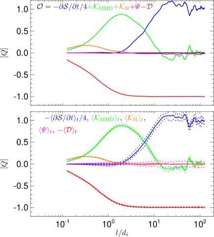
Figure 2.— KHM analysis: (top) The validity test of the compressible KHM $\mathcal{O}$, Eq. (14) (black line), as a function of $l$ at $t=255\Omega_{i}^{-1}$ along with the different contributing terms: (blue) the decay $-{\partial\mathcal{S}}/{\partial t}/4$, (green) the MHD cascade $\mathcal{K}_{\text{MHD}}$, (orange) the Hall cascade $\mathcal{K}_{\text{H}}$, (red) the dissipation $-\mathcal{D}$, and (magenta) the pressure-dilatation $\varPsi$. (bottom) Time-averaged ($240\leq t\Omega_{i}\leq 264$) contributing terms (solid lines) with their minimum and maximum values (dotted lines) for (blue) the decay $-\langle{\partial\mathcal{S}}/{\partial t}\rangle_{t}/4$, (green) the MHD cascade $\langle\mathcal{K}_{\text{MHD}}\rangle_{t}$, (orange) the Hall cascade $\langle\mathcal{K}_{\text{H}}\rangle_{t}$, (red) the dissipation/heating term $-\langle\mathcal{D}\rangle_{t}$, and (magenta) the pressure-dilatation $\langle\varPsi\rangle_{t}$. All the terms are normalized with respect to the total heating rate $Q$.

To check the prediction of Eq. (5) in the simulation we define the validity test as

$$\mathcal{O}=-\frac{1}{4}\frac{\partial\mathcal{S}}{\partial t}+\mathcal{K}_{\text{H}}+\mathcal{K}_{\text{MHD}}+\varPsi-\mathcal{D}.$$ (14)

The top panel of Figure 2 shows this validity check $\mathcal{O}$ in the 2D simulation at $t=255\Omega_{i}^{-1}$ as well as the contributing terms. The compressible KHM equation is very well conserved: $|\mathcal{O}|/Q<0.3~{}\%$, where $Q$ is the heating/dissipation rate at $t=255\Omega_{i}^{-1}$, $Q=Q_{\text{tot}}(255\Omega_{i}^{-1})$; henceforth we use $Q$ to normalize all the relevant quantities. At large scales, $\partial\mathcal{S}/\partial t/4-\varPsi\sim-\mathcal{D}\sim-Q$, that represents the energy conservation. The pressure-dilatation term $\varPsi$ is small. At intermediate scales the MHD cascade dominates, $\mathcal{K}_{\text{MHD}}\sim 0.85Q$. This term is mostly compensated by the dissipation term $\mathcal{D}$. At small scales the Hall cascade sets in and becomes comparable to the MHD one. One these scales the viscous and resistive dissipation also starts to act.

The pressure-dilatation effect is weak but not negligible. Since the energy exchanges owing to this effect oscillate around zero, it is interesting to look at the average behavior of the KHM equation over one period of these oscillations (see Fig. 1; cf., Hellinger et al., 2021). The bottom panel of Figure 2 displays the different terms contributing to the KHM equation averaged over such a period ($240\leq t\Omega_{i}\leq 264$) as well as their minimum and maximum values over this time (here $\langle\bullet\rangle_{t}$ denotes the time average) . The pressure-dilatation term varies within few percents of $Q$ over this period, and, on average, the effect of the pressure-dilatation effect is negligible. The terms $-{\partial\mathcal{S}}/{\partial t}/4$ and $\mathcal{K}_{\text{MHD}}$ exhibit similar variability whereas $\mathcal{K}_{\text{H}}$ and $\mathcal{D}$ are about constant.

3.1. Evolution

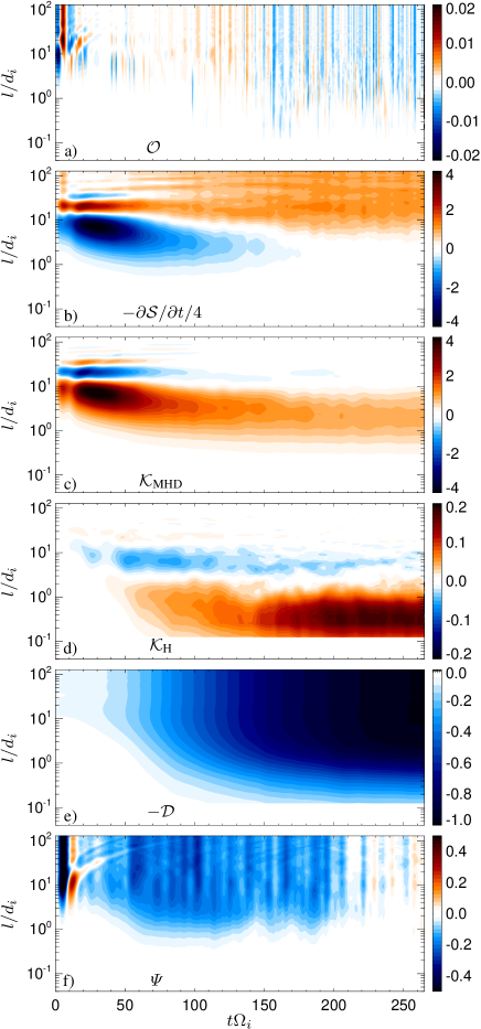
Figure 3.— Evolution of the compressible KHM law: color scale plots of (a) $\mathcal{O}$, (b) $-\partial\mathcal{S}/\partial t/4$, (c) $\mathcal{K}_{\text{MHD}}$, (d) $\mathcal{K}_{\text{H}}$, (e) $\mathcal{D}$, and (f) $\varPsi$ as functions of time and scale $l$. All the terms are normalized with respect to the total heating rate $Q$.

The compressible KHM equation is valid during the whole simulation, the homogeneity condition, $\langle(\boldsymbol{\nabla}_{\boldsymbol{x}^{\prime}}+\boldsymbol{\nabla}_{\boldsymbol{x}})\bullet\rangle=0$, is automatically satisfied for the periodic boundary conditions. Figure 3 displays the validity test $\mathcal{O}$ as well as the different contributing terms (normalized to $Q$) as functions of time and $l$. Figure 3a shows that the compressible KHM equation is well conserved, $\mathrm{max}|\mathcal{O}|/Q\lesssim 1\%$ for $t>20\Omega_{i}^{-1}$. During early times, the maximum relative error in $|\mathcal{O}|/Q$ is about $2\%$. At later times, the $|\mathcal{O}|/Q$ is below $1\%$ and is fluctuating with time and roughly constant at all scales at a given time. This is caused by numerical errors; in particular, the time derivative $\partial\mathcal{S}/\partial t$ is estimated by the finite difference with $\Delta t=\Omega_{i}^{-1}$. This is likely not sufficient for the transition from the initial superposition of large scale Alfvénic fluctuations. The interpretation is supported by the fact that $\mathcal{O}$ increases when we increase $\Delta t$.

Figure 3bc show that initially $\partial\mathcal{S}/\partial t$ and $\mathcal{K}_{\text{MHD}}$ compensate each other, $\partial\mathcal{S}/\partial t+4\mathcal{K}_{\text{MHD}}\sim 0$. $\partial\mathcal{S}/\partial t$ evolves and, at later times, dominates at large scales indicating a decay of the kinetic + magnetic energy at large scales. $\mathcal{K}_{\text{MHD}}$ becomes dominant at intermediate scales. Figure 3d shows that the Hall term becomes important at $40\lesssim t\Omega_{i}\lesssim 60$ for $l\lesssim 3d_{i}$; this is about the time when thin current sheets form and start to reconnect (Papini et al., 2019a). Interestingly, there is an indication of a negative Hall cascade rate, starting earlier $40\lesssim t\Omega_{i}$ for $3d_{i}\lesssim l\lesssim 20$, indicating an energy transfer from small to large scales, that may be part of the onset of turbulence (cf., Franci et al., 2017). The Hall term settles to the asymptotic value after $t\simeq 150$, when the energy at large scales has had time to participate to the cascade.

Figure 3e demonstrates that the dissipation gradually develops as the (MHD and Hall) cascade evolves and brings energy to small scales. Figure 3f displays the pressure-dilatation term $\varPsi$. After the initial transition, this term is important on relatively large scales for a long time; its negative value indicates a compressible plasma heating. Then it becomes weakly oscillating around zero for $t\gtrsim 210\Omega_{i}^{-1}$.

Note that the alternative KHM equation, Eq. (7), gives, unsurprisingly, almost the same results as Eq. (4). The cascade rates $\mathcal{K}_{\text{MHD}}$ and $\mathcal{K}_{\text{H}}$ differ within $10^{-3}Q$ between the two methods. On the other hand, for the weakly-compressible simulation, the incompressible approximation (Hellinger et al., 2018; Ferrand et al., 2019) exhibits an error that is mostly related to the neglected pressure-dilatation term. However, the incompressible MHD and Hall cascade rates are close to their compressible counterparts (not shown).

4. Spectral Transfer

Another way to analyze the scale dependence of turbulence and its processes is the spectral (Fourier) decomposition. To characterize the kinetic energy in the compressible flow one can use the density-weighted velocity field $\boldsymbol{w}$ as in the KHM approach. The evolution for the energy in a given Fourier mode

$$\widehat{\boldsymbol{w}}(\boldsymbol{k}) =\sum_{\boldsymbol{x}}\boldsymbol{w}(\boldsymbol{x})\mathrm{exp}(i\boldsymbol{k}\cdot\boldsymbol{x}),$$ (15)

$$\widehat{\boldsymbol{B}}(\boldsymbol{k}) =\sum_{\boldsymbol{x}}\boldsymbol{B}(\boldsymbol{x})\mathrm{exp}(i\boldsymbol{k}\cdot\boldsymbol{x})$$ (16)

follows from Eqs. (1–3) (cf., Mininni et al., 2007; Grete et al., 2017)

$$\frac{1}{2}\frac{\partial\left(|\widehat{\boldsymbol{w}}|^{2}+|\widehat{\boldsymbol{B}}|^{2}\right)}{\partial t}= -T_{\text{MHD}}-T_{\text{H}}-\Re\widehat{\boldsymbol{w}}^{*}\cdot\widehat{\frac{\boldsymbol{\nabla}p}{\sqrt{\rho}}}$$

$$+\Re\widehat{\boldsymbol{w}}^{*}\cdot\widehat{\frac{\boldsymbol{\nabla}\cdot\boldsymbol{\tau}}{\sqrt{\rho}}}-\eta k^{2}|\widehat{\boldsymbol{B}}|^{2},$$ (17)

where the MHD and Hall transfer terms are

$$T_{\text{MHD}}= \Re\bigg{[}\widehat{\boldsymbol{w}}^{*}\cdot\widehat{(\boldsymbol{u}\cdot\boldsymbol{\nabla})\boldsymbol{w}}+\frac{1}{2}\widehat{\boldsymbol{w}}^{*}\cdot\widehat{\boldsymbol{w}\theta}$$

$$-\widehat{\boldsymbol{w}}^{*}\cdot\widehat{\frac{(\boldsymbol{\nabla}\times\boldsymbol{B})\times\boldsymbol{B}}{\sqrt{\rho}}}-\widehat{\boldsymbol{B}}^{*}\cdot\widehat{\boldsymbol{\nabla}\times\left(\boldsymbol{u}\times\boldsymbol{B}\right)}\bigg{]},$$

$$T_{\text{H}}= \Re\bigg{[}\widehat{\boldsymbol{B}}^{*}\cdot\widehat{\boldsymbol{\nabla}\times\left(\boldsymbol{j}\times\boldsymbol{B}\right)}\bigg{]},$$

respectively; here wide hat denotes the Fourier transform, the star denotes the complex conjugate, and $\Re$ denotes the real part.

In the inertial range, one expects that the time-derivative terms in Eq. (17) are zero and the same is expected for the dissipation and pressure-dilatation terms. The transfer term $T_{\text{MHD}}+T_{\text{H}}$ is also expected to be zero, as all the energy that arrives from larger scales proceeds to smaller scales. To characterize (isotropic) turbulence we use a low-pass filtered kinetic + magnetic energy (i.e., the energy in modes with wave-vector magnitudes smaller than or equal to $k$, cf., Hellinger et al., 2021)

$$E_{k} =\frac{1}{2}\sum_{|\boldsymbol{k}^{\prime}|\leq k}\left(|\widehat{\boldsymbol{w}}|^{2}+|\widehat{\boldsymbol{B}}|^{2}\right).$$ (18)

For $E_{k}$ one gets the following dynamic equation

$$\frac{\partial E_{k}}{\partial t}+S_{\text{MHD}k}+S_{\text{H}k}=\Psi_{k}-D_{k}$$ (19)

where

$$S_{\text{MHD}k} =\sum_{|\boldsymbol{k}^{\prime}|\leq k}T_{\text{MHD}}(\boldsymbol{k}^{\prime}),\ \ \ S_{\text{H}k}=\sum_{|\boldsymbol{k}^{\prime}|\leq k}T_{\text{H}}(\boldsymbol{k}^{\prime}),$$ (20)

$$\Psi_{k} =-\sum_{|\boldsymbol{k}^{\prime}|\leq k}\widehat{\boldsymbol{w}}^{*}\cdot\widehat{\rho^{-1/2}\boldsymbol{\nabla}p},$$ (21)

$$D_{k} =\eta\sum_{|\boldsymbol{k}^{\prime}|\leq k}{k^{\prime}}^{2}|\widehat{\boldsymbol{B}}|^{2}-\sum_{|\boldsymbol{k}^{\prime}|\leq k}\widehat{\boldsymbol{w}}^{*}\cdot\widehat{\rho^{-1/2}\boldsymbol{\nabla}\cdot\boldsymbol{\tau}}.$$ (22)

Here $S_{\text{MHD}k}$ and $S_{\text{H}k}$ represent the MHD and Hall energy transfer rates, respectively, $\Psi_{k}$ describes the pressure-dilatation effect, and $D_{k}$ is the (viscous and resistive) dissipation rate for modes with wave-vector magnitude smaller than or equal to $k$. When $S_{\text{MHD}k}$ or $S_{\text{H}k}$ are constant, the corresponding energy transfer rate is constant, and can be identified with the cascade rate. For large wave vectors, one gets the unfiltered values

$$E_{k}\rightarrow E_{\text{kin}}+E_{\text{mag}},\ \ \ \Psi_{k}\rightarrow\langle p\theta\rangle,\ \ \text{and}\ \ D_{k}\rightarrow Q,$$ (23)

To check the spectral transfer of energy given by Eq. (19), we define the validity test (similarly to Eq. (14)) as

$$O_{k}=\frac{\partial E_{k}}{\partial t}+S_{\text{MHD}k}+S_{\text{H}k}-\Psi_{k}+D_{k}$$ (24)

Fig. 4 (top panel) shows the validity test and the contributing terms as functions of $k$ at $t=255\Omega_{i}^{-1}$. Eq. (19) is well satisfied, $|O_{k}|/Q<0.3~{}\%$. At large scales, small positive values of $\partial E_{k}/\partial t$ compensated by $S_{\text{MHD}k}$ indicate an inverse cascade/energy transfer from small to large scales. At medium scales, the MHD cascade term dominates, reaching the maximum value about $0.85Q$; the MHD cascade term is compensated mostly by $\partial E_{k}/\partial t$. At small scales, the Hall cascade sets in but, at the same time, the dissipation gets important and a weak pressure-dilatation effect appears. For large $k$ one recovers the energy conservation

$$\frac{\partial(E_{\text{kin}}+E_{\text{mag}})}{\partial t}=\langle p\theta\rangle-Q.$$ (25)

As in the KHM case, it is interesting to look at the properties of the ST equation averaged over one period of the pressure-dilatation oscillation. Fig. 4 (bottom panel) displays the terms contributing to the ST equation (Eq. 19) averaged over the time interval $240\leq t\Omega_{i}\leq 264$ along with their minimum and maximum values. The pressure-dilatation term $\Psi_{k}$ exhibits a variation of few percents of $Q$ and, on average, it is negligible. The decay $\partial E_{k}/\partial t$ and the MHD cascade $S_{\text{MHD}k}$ have also a similar variability whereas the Hall cascade $S_{\text{H}k}$ and the dissipation $D_{k}$ tend to be about constant during the oscillation period.

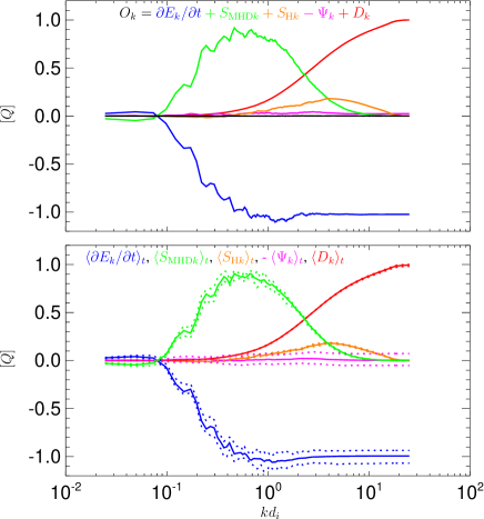
Figure 4.— Spectral transfer analysis: (top) The validity test of the compressible ST $O_{k}$, Eq. (24), (black line) as a function of $k$ at $t=255\Omega_{i}^{-1}$ along with the different contributing terms: (blue) the decay $\partial E_{k}/\partial t$, (green) the MHD cascade $S_{\text{MHD}k}$, (orange) the Hall cascade $S_{\text{H}k}$, (red) the dissipation $D_{k}$ , and (magenta) the pressure-dilatation term $-\Psi_{k}$. (bottom) Time-averaged contributing terms (solid lines) with their minimum and maximum values (dotted lines) for (blue) the decay $\langle\partial E_{k}/\partial t\rangle_{t}$, (green) the MHD cascade $\langle S_{\text{MHD}k}\rangle_{t}$, (orange) the Hall cascade $\langle S_{\text{H}k}\rangle_{t}$, (red) the dissipation $\langle D_{k}\rangle_{t}$ , and (magenta) the pressure-dilatation term $-\langle\Psi_{k}\rangle_{t}$. All the quantities are given in units of the total heating rate $Q$.

The ST equation is valid during the whole simulation owing to the peridic boundary condisions as in the case of the KHM equation. Figure 5 displays the evolution of the ST equation in the simulation in a format similar to that of Fig. 3.

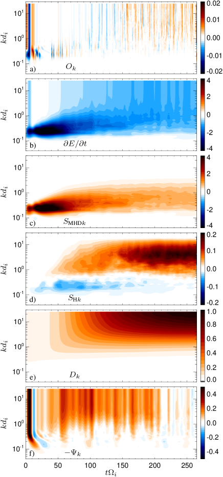
Figure 5.— Evolution of the compressible ST law: color scale plots of (a) $O_{k}$, (b) $\partial E_{k}/\partial t/4$, (c) $S_{\text{MHD}k}$, (d) $S_{\text{H}k}$, (e) $D_{k}$, and (f) $-\Psi_{k}$ as functions of time and scale $l$. Dotted lines denote the injection scale $kd_{i}=0.2$. All the terms are normalized with respect to the total heating rate $Q$.

Figure 5 shows that the ST and KHM equations give similar results. Note, moreover, that a good quantitative agreement between the two approaches appears at later times when turbulence is well developed.

4.1. Comparison between KHM and ST approaches

The KHM and ST equations give similar results. They are empirically related through the inverse proportionality between the wave vector $k$ and the spatial separation length $l$ as $kl\simeq\sqrt{2}$.

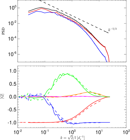
Figure 6.— (top) The power spectra of the velocity (blue), magnetic field (red), and the total power spectrum as functions of $k$ at $t=255\Omega_{i}^{-1}$. (bottom) Solid lines show the contributing terms of the ST equation (averaged over $240\leq t\Omega_{i}\leq 264$, see Fig. 4, bottom) as function of $k$: (blue) the decay $\langle\partial E_{k}/\partial t\rangle_{t}$, (green) the MHD cascade $\langle S_{\text{MHD}k}\rangle_{t}$, (orange) the Hall cascade $\langle S_{\text{H}k}\rangle_{t}$, (red) the dissipation $\langle D_{k}\rangle_{t}-Q$ , and (magenta) the pressure-dilatation term $-\langle\Psi_{k}\rangle_{t}$. Dashed lines show the corresponding time-averaged results of the KHM equation (see Fig. 2, bottom) as function of $k$ through the relation $l=\sqrt{2}/k$: (blue) the decay $-\langle{\partial\mathcal{S}}/{\partial t}\rangle_{t}/4-Q$, (green) the MHD cascade $\langle\mathcal{K}_{\text{MHD}}\rangle_{t}$, (orange) the Hall cascade $\langle\mathcal{K}_{\text{H}}\rangle_{t}$, (red) the dissipation $-\langle\mathcal{D}\rangle_{t}$, and (magenta) the pressure-dilatation $\langle\varPsi\rangle_{t}$. All the quantities are given in units of the total dissipation rate $Q$. Note that some terms are shifted by $-Q$ with respect to Figs. 2 and 4.

The top panel of Fig. 6 shows the power spectra of the velocity (blue), magnetic field (red), and the total power spectrum as functions of $k$ (at $t=255\Omega_{i}^{-1}$) as a reference. The dashed line denotes a $k^{-5/3}$ power law for comparison.

The bottom panel Fig. 6 displays a direct comparison between the ST and KHM contributing terms as functions of $k$ (through the inverse proportionality $kl=\sqrt{2}$). Fig. 6 shows that the MHD and Hall cascade rates in both the approaches are comparable $\langle S_{\text{MHD}k}\rangle_{t}\simeq\langle\mathcal{K}_{\text{MHD}}\rangle_{t}$, $\langle S_{\text{H}k}\rangle_{t}\simeq\langle\mathcal{K}_{\text{H}}\rangle_{t}$. Note that the MHD cascade term dominates at scales where the total power spectrum is close to a $k^{-5/3}$ power law. The average pressure-dilation effect is negligible. Similarly to the hydrodynamic case (Hellinger et al., 2021), the ST and KHM approaches are complementary:

$$\langle\partial E_{k}/\partial t\rangle_{t}+\langle{\partial\mathcal{S}}/{\partial t}\rangle_{t}/4 \simeq-Q$$ (26)

$$\langle D_{k}\rangle_{t}+\langle\mathcal{D}\rangle_{t}\simeq Q$$ (27)

$\partial E_{k}/{\partial t}$ represents the rate of change of the kinetic energy at scales with wave-vector magnitudes smaller or equal to $k$ whereas ${\partial\mathcal{S}}/{\partial t}/4$ represents approximatively the rate for wave-vector magnitudes larger than $k$. Similarly, $D_{k}$ is the dissipation rate on the scales $\leq k$ whereas $\mathcal{D}$ represents the dissipation rate on the scales $>k$.

5. Reduced, one-dimensional analyses

In the present simulation, due to the reduced dimensionality, we cannot address the question of the spectral anisotropy (Verdini et al., 2015). We can, however, test what estimates of the cascade rate we can get from 1D cuts representing observed 1D time series. We take 1D cuts (both in $x$ and $y$ direction) to calculate the ST predictions $S_{\text{MHD}}^{(\text{1D})}$ and $S_{\text{H}}^{(\text{1D})}$ and the KHM predictions $\mathcal{K}_{\text{MHD}}^{(\text{1D})}$ and $\mathcal{K}_{\text{H}}^{(\text{1D})}$.

For the reduced 1D ST equation we take 1D Fourier transform in Eq. (19) and we retain all the spatial derivatives, and, similarly, we use all the spatial derivatives (in the real space) for the alternative KHM equation. On the other hand, for the standard KHM equation, Eq. (4), only the derivative along the 1D direction in the separation space $l$ is used to estimate $\boldsymbol{\nabla}\cdot(\boldsymbol{\mathcal{Y}}+\boldsymbol{\mathcal{H}})$. Results from these estimates are shown in Fig. 7. This figure shows the MHD and Hall cascade rates obtained from the reduced 1D analyses as functions of $k$ for the ST approach and $k=1/l$ for the KHM approaches. The calculation is done for the time $t=255\Omega_{i}^{-1}$, see top panels of Figs. 4 and 2. The reduced ST equation gives the cascade rates relatively similar to those obtained from the whole simulation domain. On the other hand, the reduced 1D results based on the standard KHM equation, Eq. (4), are quite different from the full results: the maximum value of the MHD cascade rate is notable about half the expected value. This can be partly amended by assuming isotropy, $\boldsymbol{\nabla}\cdot\boldsymbol{\mathcal{Y}}\sim 2\partial\mathcal{Y}_{l}/\partial l$. However, even after this correction the agreement between the 1D ST and standard KHM method is poor. Interestingly, the reduced 1D results based on the alternative KHM equation, Eq. (7), are in a good agreement with the full results, as well as with the results of the reduced 1D ST equation. This likely related to the fact that for the alternative, divergence-less formulation we use higher-dimensionality derivatives that correspond to the divergence in the standard KHM equation. Finally, we note that the agreement between the 1D ST and KHM results appears for $kl=\alpha$, where $\alpha\sim 1$.

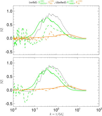
Figure 7.— Reduced 1-D analyses of (green) MHD and (orange) Hall cascade rates (see the text for details): Solid lines show the ST cascade rates $S_{\text{MHD}}^{(\text{1D})}$ and $S_{\text{H}}^{(\text{1D})}$ as functions of $k$, estimated from 1D cuts using Eq. (19). Dashed lines displays the cascade rates $\mathcal{K}_{\text{MHD}}^{(\text{1D})}$ and $\mathcal{K}_{\text{H}}^{(\text{1D})}$ as functions of $k=1/l$ estimated from 1D cuts using the standard KHM equation, Eq. (4), in the top panel, whereas in the bottom panel they denote the cascade rates estimated using the alternative KHM equation, Eq. (7). Dotted lines displays the MHD cascade rate $S_{\text{MHD}}$ from the full analysis (see Fig. 4, top panel) for comparison. All the quantities are given in units of the total heating rate $Q$.

6. Discussion

In this paper we derived two new forms of the KHM equation for compressible Hall MHD turbulence. We tested these equations, along with an isotropic ST equation, on the results of a 2D Hall MHD simulation of weakly compressible turbulence with a moderate Reynolds number. The KHM and ST equations are well satisfied in the simulation cross-validating these equations and simulation results. The two KHM equations give the same results and they are equivalent and complementary to the ST equation via the inverse proportionality $kl=\alpha$ with $\alpha\simeq\sqrt{2}$. Note that a similar correspondence is observed in three-dimensional (3D) HD turbulence (Hellinger et al., 2021) for $\alpha\simeq\sqrt{3}$ and preliminary results of isotropic (unmagnetized) 3D Hall MHD turbulence suggest the same relationship. In the reduced, 1D analyses we observe $\alpha\simeq 1$. This indicates that the relationship between the ST and KHM equation $kl=\alpha$ depends on the dimensionality $d$ of the analyzed space, $\alpha\simeq\sqrt{d}$. This simple relationship is useful to interpret the KMH results in the context of spectral analyses. Equations analogous to the ST and KHM ones can be obtained using the low-pass filtering/coarse graining of the energy conservation laws (Eyink & Aluie, 2009; Aluie, 2011, 2013; Yang et al., 2016, 2017; Camporeale et al., 2018).

The KHM and ST equations are valid during the whole simulation, owing to the periodic boundary conditions and they can be used to analyze the onset of turbulence. The agreement between the two approaches is at least qualitative during the whole simulation but only at later times, when turbulence is well developed, there is a good quantitative agreement; this indicates that the KHM and ST approaches become equivalent when turbulence is well developed and the energy transfer is expected be local so that one can talk about the energy cascade. The simulation results suggest that the onset of the Hall cascade is related to formation of reconnecting current sheets (Papini et al., 2019a) and that, at least during the onset, the Hall term leads to an energy transfer from small to large scales at a range of scales above $d_{i}$ (cf., Franci et al., 2017); at this stage, this transfer is likely not local and one cannot speak about a energy cascade. The locality can be tested using a (spectral) shell-to-shell transfer analysis (Alexakis et al., 2005). For the weakly compressible simulation, the incompressible approximation is not correct to a large extent due to the neglected pressure-dilatation effect. This error is important during the turbulence onset. When turbulence is well developed, the time-averaged pressure-dilatation becomes negligible, and the compressible and incompressible KHM predictions for MHD and Hall cascade rates are close to each other.

It is interesting to note that the standard compressible KHM equation, Eq. (4), does not depend (except for the correction term $\mathcal{C}$) on the background magnetic field $\boldsymbol{B}_{0}=\langle\boldsymbol{B}\rangle$ similarly to the incompressible case (Oughton et al., 2013). On the other hand, there is in principle a contribution from the mean fluid velocity $\boldsymbol{u}_{0}=\langle\boldsymbol{u}\rangle$ (Hadid et al., 2017). In the incompressible, constant-density limit one recovers the incompressible results (Hellinger et al., 2018; Ferrand et al., 2019; Banerjee & Galtier, 2017).

There is a couple of differences between our standard KHM equation (Eq. (4)) and that of Andrés et al. (2018): We describe the kinetic energy by the structure function $\langle|\delta\boldsymbol{w}|^{2}\rangle$ that guarantee positive values in contrast with $\langle\delta(\rho\boldsymbol{u})\cdot\delta\boldsymbol{u}\rangle$. Similarly, we represent the magnetic energy contribution by the structure function $S_{B}=\langle|\delta\boldsymbol{B}|^{2}\rangle$ instead of $\langle\delta(\rho^{1/2}\boldsymbol{B})\cdot\delta(\boldsymbol{B}/\rho^{1/2})\rangle$. This difference is very likely not substantial. In the case of compressible HD turbulence, the corresponding two approaches give very similar results (Hellinger et al., 2021). However, the important difference between our results and those of Andrés et al. (2018) is that we formulate the KHM equations for the kinetic + magnetic energy. The simulation results exhibit no net energy exchange between the kinetic + magnetic energy and the internal one for later times when turbulence is well developed and the pressure-dilation effect does not lead to cross-scale energy transfer (cf., Aluie et al., 2012). The inclusion of the internal energy into the KHM equation (Andrés et al., 2018, and references therein) is therefore not needed. Moreover, the HD results of Hellinger et al. (2021) indicate that it is hard to represent the kinetic energy and the internal one by compatible structure functions. Furthermore, Andrés et al. (2018) use the isothermal closure to modify the description of the pressure-dilatation effect; this closure is not generally applicable. Finally, estimates of the energy cascade rate in the solar wind based on such approaches (Banerjee et al., 2016; Hadid et al., 2017; Andrés et al., 2019) include the scale redistribution of the internal energy and cannot be simply related to the plasma heating rates (cf., MacBride et al., 2008).

For our study, we used one 2D Hall MHD simulation of weakly compressible turbulence for a moderated Reynolds number and zero cross-helicity. This was sufficient for testing and comparing the KHM and ST equations, but our results need to be extended to more compressible and/or larger system that extends further to the Hall range of scales, and/or to systems with larger cross (canonical) helicity, etc. Our results need to be extended to 3D in order to investigate the anisotropy of the turbulent cascade. Both the KHM equations can be naturally used (cf., Verdini et al., 2015). However, it is not clear how to extend the isotropic ST approach to an anisotropic situation (cf., Verma, 2017); the low-pass filtering/coarse graining approaches also usually assume isotropy.

The Hall cascade rate in the simulation is a fraction of the MHD one because of the dissipation. In both kinetic simulations and in-situ observations the situation is similar (Bandyopadhyay et al., 2020b). The decrease of the cascade rate from the MHD to the Hall range is likely due to some sort of dissipation/particle energization. The present work assumes a scalar pressure $p$ that is relevant for collision-dominated plasmas. In weakly collisional/collisionless systems, such as in the solar wind, it is necessary to employ the full pressure tensor $\boldsymbol{\mathrm{P}}$ and to replace the pressure-dilatation coupling, $p\theta$, by the pressure-strain one, $\boldsymbol{\mathrm{P}}:\boldsymbol{\Sigma}$, (Yang et al., 2019; Matthaeus et al., 2020). The KHM and ST approaches can be easily generalized to account for the pressure tensor. For instance, $\langle\delta p\delta\theta\rangle$ becomes simply $\langle\delta\boldsymbol{\mathrm{P}}:\delta\boldsymbol{\Sigma}\rangle$ (see the viscous dissipation term).

Our reduced 1D analysis suggests that the ST equation and the alternative KHM equation give better estimations of the cascade rate from in situ observed time series compared to the usually used standard KHM. However, this is likely owing to the usage of multi-dimensional spatial derivatives that may possibly be only estimated using multi-point data of Cluster or MMS missions. Furthermore, the ST equation is formulated for an isotropic situation. Nevertheless, we believe that the ST and alternative KHM approaches are worth pursuing as they provide other methods for measuring the energy cascade rates from in situ observations.

Appendix A Derivation of the standard KHM equation

We start by reformulating the compressible Hall MHD equation in terms of $\boldsymbol{w}=\rho^{1/2}\boldsymbol{u}$.

$$\frac{\partial\boldsymbol{w}}{\partial t} +(\boldsymbol{u}\cdot\boldsymbol{\nabla})\boldsymbol{w}+\frac{\boldsymbol{w}\theta}{2}=\frac{\boldsymbol{f}}{\sqrt{\rho}}$$ (A1)

$$\frac{\partial\boldsymbol{B}}{\partial t} +(\boldsymbol{u}\cdot\boldsymbol{\nabla})\boldsymbol{B}=(\boldsymbol{B}\cdot\boldsymbol{\nabla})\boldsymbol{u}-\boldsymbol{B}\theta+\eta\Delta\boldsymbol{B}+\boldsymbol{h}$$ (A2)

where we denoted

$$\boldsymbol{f} =(\boldsymbol{\nabla}\times\boldsymbol{B})\times\boldsymbol{B}-\boldsymbol{\nabla}p+\boldsymbol{\nabla}\cdot\boldsymbol{\tau}$$ (A3)

$$\boldsymbol{h} =-(\boldsymbol{B}\cdot\boldsymbol{\nabla})\boldsymbol{j}+(\boldsymbol{j}\cdot\boldsymbol{\nabla})\boldsymbol{B}+\boldsymbol{B}\left(\boldsymbol{\nabla}\cdot\boldsymbol{j}\right).$$ (A4)

We take the Hall MHD equations at two different points, $\boldsymbol{x}^{\prime}=\boldsymbol{x}+\boldsymbol{l}$ and $\boldsymbol{x}$ and subtract them to get

$$\frac{\partial\delta\boldsymbol{w}}{\partial t} +(\delta\boldsymbol{u}\cdot\boldsymbol{\nabla}^{\prime})\delta\boldsymbol{w}+\left[\boldsymbol{u}\cdot\left(\boldsymbol{\nabla}+\boldsymbol{\nabla}^{\prime}\right)\right]\delta\boldsymbol{w}$$

$$+\frac{1}{2}(\boldsymbol{w}^{\prime}\theta^{\prime}-\boldsymbol{w}\theta)=\delta\left(\frac{\boldsymbol{f}}{\sqrt{\rho}}\right)$$ (A5)

where we denote $a=a(\boldsymbol{x})$, $a^{\prime}=a(\boldsymbol{x}^{\prime})$, and $\delta a=a^{\prime}-a$ for any variable $a$; analogically, $\boldsymbol{\nabla}=\boldsymbol{\nabla}_{\boldsymbol{x}}$, $\boldsymbol{\nabla}^{\prime}=\boldsymbol{\nabla}_{\boldsymbol{x}^{\prime}}$ and $\Delta=\Delta_{\boldsymbol{x}}$, $\Delta^{\prime}=\Delta_{\boldsymbol{x}^{\prime}}$, $\Delta$ being the Laplace operator. Here and henceforth this relationship is repeatedly applied (Carbone et al., 2009)

$$\delta\left[(\boldsymbol{a}\cdot\boldsymbol{\nabla})\boldsymbol{b}\right] =(\boldsymbol{a}^{\prime}\cdot\boldsymbol{\nabla}^{\prime})\boldsymbol{b}^{\prime}-(\boldsymbol{a}\cdot\boldsymbol{\nabla})\boldsymbol{b}$$

$$=(\boldsymbol{a}^{\prime}\cdot\boldsymbol{\nabla}^{\prime})\delta\boldsymbol{b}+(\boldsymbol{a}\cdot\boldsymbol{\nabla})\delta\boldsymbol{b}$$

$$=(\delta\boldsymbol{a}\cdot\boldsymbol{\nabla}^{\prime})\delta\boldsymbol{b}+[\boldsymbol{a}\cdot(\boldsymbol{\nabla}+\boldsymbol{\nabla}^{\prime})]\delta\boldsymbol{b},$$ (A6)

and $\boldsymbol{x}$ and $\boldsymbol{x}^{\prime}$ are assumed to be independent, i.e., $\boldsymbol{\nabla}^{\prime}\boldsymbol{a}=\boldsymbol{\nabla}\boldsymbol{a}^{\prime}=0$ for any $\boldsymbol{a}$.

$$\frac{\partial|\delta\boldsymbol{w}|^{2}}{\partial t} +\boldsymbol{\nabla}^{\prime}\cdot\left(\delta\boldsymbol{u}|\delta\boldsymbol{w}|^{2}\right)+\left(\boldsymbol{\nabla}+\boldsymbol{\nabla}^{\prime}\right)\cdot\left(\boldsymbol{u}|\delta\boldsymbol{w}|^{2}\right)$$ (A7)

$$+\delta\boldsymbol{w}\cdot\left(\theta^{\prime}\boldsymbol{w}-\theta\boldsymbol{w}^{\prime}\right)=2\delta\boldsymbol{w}\cdot\delta\left(\frac{\boldsymbol{f}}{\sqrt{\rho}}\right)$$ (A8)

Taking a spatial average

$$\frac{\partial\mathcal{S}_{w}}{\partial t}+\boldsymbol{\nabla}_{\boldsymbol{l}}\cdot\left\langle\delta\boldsymbol{u}|\delta\boldsymbol{w}|^{2}\right\rangle+\mathcal{R}=2\left\langle\delta\boldsymbol{w}\cdot\delta\left(\frac{\boldsymbol{f}}{\sqrt{\rho}}\right)\right\rangle$$ (A9)

where $\mathcal{S}_{w}=\langle|\delta\boldsymbol{w}|^{2}\rangle$ and $\mathcal{R}=\langle\delta\boldsymbol{w}\cdot\left(\theta^{\prime}\boldsymbol{w}-\theta\boldsymbol{w}^{\prime}\right)\rangle$. Here we assume that the system is homogeneous, i.e.,

$$\langle\left(\boldsymbol{\nabla}+\boldsymbol{\nabla}^{\prime}\right)\cdot\boldsymbol{a}\rangle=0$$ (A10)

for any quantity $\boldsymbol{a}$ (Frisch, 1995).

Similarly for the magnetic field we have

$$\frac{\partial|\delta\boldsymbol{B}|^{2}}{\partial t} +\boldsymbol{\nabla}^{\prime}\cdot\left(\delta\boldsymbol{u}|\delta\boldsymbol{B}|^{2}\right)+\left(\boldsymbol{\nabla}+\boldsymbol{\nabla}^{\prime}\right)\cdot\left(\boldsymbol{u}|\delta\boldsymbol{B}|^{2}\right)$$

$$=2\delta\boldsymbol{B}\cdot(\delta\boldsymbol{B}\cdot\boldsymbol{\nabla}^{\prime})\delta\boldsymbol{u}+\left(B^{\prime 2}-B^{2}\right)\left(\theta-\theta^{\prime}\right)$$

$$+2\delta\boldsymbol{B}\cdot\left[\boldsymbol{B}\cdot\left(\boldsymbol{\nabla}+\boldsymbol{\nabla}^{\prime}\right)\right])\delta\boldsymbol{u}$$

$$+2\eta\delta\boldsymbol{B}\cdot\left(\Delta^{\prime}\boldsymbol{B}^{\prime}-\Delta\boldsymbol{B}\right)+2\delta\boldsymbol{B}\cdot\delta\boldsymbol{h}$$ (A11)

Taking the spatial average

$$\frac{\partial\mathcal{S}_{B}}{\partial t} +\boldsymbol{\nabla}_{\boldsymbol{l}}\cdot\left\langle\delta\boldsymbol{u}|\delta\boldsymbol{B}|^{2}\right\rangle-2\left\langle\delta\boldsymbol{B}\cdot(\delta\boldsymbol{B}\cdot\boldsymbol{\nabla}^{\prime})\delta\boldsymbol{u}\right\rangle$$

$$=-\left\langle\delta\left(B^{2}\right)\delta\theta\right\rangle+2\left\langle\delta\boldsymbol{B}\cdot\left[\boldsymbol{B}\cdot\left(\boldsymbol{\nabla}+\boldsymbol{\nabla}^{\prime}\right)\right])\delta\boldsymbol{u}\right\rangle$$

$$-4Q_{\eta}+2\eta\Delta_{\boldsymbol{l}}S_{B}+2\left\langle\delta\boldsymbol{B}\cdot\delta\boldsymbol{h}\right\rangle$$ (A12)

where $S_{B}=\langle|\delta\boldsymbol{B}|^{2}\rangle$, $Q_{\eta}=\eta\langle\boldsymbol{\nabla}\boldsymbol{B}:\boldsymbol{\nabla}\boldsymbol{B}\rangle=\eta\langle J^{2}\rangle.$ In order to derive an equation for the structure function $\mathcal{S}=\mathcal{S}_{w}+\mathcal{S}_{B}$ and to obtain a simple equation we introduce a correction term $\mathcal{C}_{\text{MHD}}=2\langle\delta\boldsymbol{w}\cdot\delta\left(\rho^{-1/2}\boldsymbol{f}\right)\rangle-2\langle\delta\boldsymbol{u}\cdot\delta\boldsymbol{f}\rangle.$ The last term can be expressed as

$$2\left\langle\delta\boldsymbol{u}\cdot\delta\boldsymbol{f}\right\rangle =2\left\langle\delta\boldsymbol{u}\cdot\left(\boldsymbol{B}\cdot\left(\boldsymbol{\nabla}+\boldsymbol{\nabla}^{\prime}\right)\right)\delta\boldsymbol{B}\right\rangle$$

$$+2\left\langle\delta\boldsymbol{u}\cdot\left(\delta\boldsymbol{B}\cdot\boldsymbol{\nabla}^{\prime}\right)\delta\boldsymbol{B}\right\rangle-\left\langle\delta\boldsymbol{u}\cdot\delta\left(\boldsymbol{\nabla}B^{2}\right)\right\rangle$$

$$+2\left\langle\delta\theta\delta p\right\rangle-2\left\langle\delta\boldsymbol{\Sigma}:\delta\boldsymbol{\tau}\right\rangle.$$ (A13)

Combining the previous results we get for $\mathcal{S}$

$$\frac{\partial\mathcal{S}}{\partial t}+\boldsymbol{\nabla}_{\boldsymbol{l}}\cdot\boldsymbol{\mathcal{Y}}+\mathcal{R} =\mathcal{C}_{\text{MHD}}+2\left\langle\delta\theta\delta p\right\rangle-2\left\langle\delta\boldsymbol{\Sigma}:\delta\boldsymbol{\tau}\right\rangle$$

$$-4Q_{\eta}+2\eta\Delta_{\boldsymbol{l}}\mathcal{S}_{B}+2\langle\delta\boldsymbol{B}\cdot\delta\boldsymbol{h}\rangle$$ (A14)

where $\boldsymbol{\mathcal{Y}}=\left\langle\delta\boldsymbol{u}\left(|\delta\boldsymbol{w}|^{2}+|\delta\boldsymbol{B}|^{2}\right)-2\delta\boldsymbol{B}\left(\delta\boldsymbol{B}\cdot\delta\boldsymbol{u}\right)\right\rangle$

To finish the calculation we need to evaluated the Hall contribution $2\langle\delta\boldsymbol{B}\cdot\delta\boldsymbol{h}\rangle$. First, for $\delta\boldsymbol{h}$ is easy to get

$$\delta\boldsymbol{h} =-(\delta\boldsymbol{B}\cdot\boldsymbol{\nabla}^{\prime})\delta\boldsymbol{j}-(\boldsymbol{B}\cdot\left(\boldsymbol{\nabla}+\boldsymbol{\nabla}^{\prime}\right))\delta\boldsymbol{j}$$

$$+(\delta\boldsymbol{j}\cdot\boldsymbol{\nabla}^{\prime})\delta\boldsymbol{B}+(\boldsymbol{j}\cdot\left(\boldsymbol{\nabla}+\boldsymbol{\nabla}^{\prime}\right))\delta\boldsymbol{B}$$

$$+\delta\boldsymbol{B}\left(\boldsymbol{\nabla}^{\prime}\cdot\delta\boldsymbol{j}\right)+\boldsymbol{B}\left(\left[\boldsymbol{\nabla}+\boldsymbol{\nabla}^{\prime}\right]\cdot\delta\boldsymbol{j}\right)$$ (A15)

The term $2\langle\delta\boldsymbol{B}\cdot\delta\boldsymbol{h}\rangle$ may be then given in the form (Hellinger et al., 2018; Ferrand et al., 2019)

$$2\left\langle\delta\boldsymbol{B}\cdot\delta\boldsymbol{h}\right\rangle=-2\boldsymbol{\nabla}_{\boldsymbol{l}}\cdot\boldsymbol{\mathcal{H}}+2\mathcal{A}$$ (A16)

where

$$\boldsymbol{\mathcal{H}} =\left\langle\delta\boldsymbol{B}\left(\delta\boldsymbol{B}\cdot\delta\boldsymbol{j}\right)-\delta\boldsymbol{j}\left|\delta\boldsymbol{B}\right|^{2}/2\right\rangle$$

$$=\left\langle\delta\boldsymbol{B}\times\left(\delta\boldsymbol{B}\times\delta\boldsymbol{j}\right)+\delta\boldsymbol{j}\left|\delta\boldsymbol{B}\right|^{2}/2\right\rangle$$ (A17)

and

$$\mathcal{A}=\left\langle\boldsymbol{j}\cdot\left(\boldsymbol{B}^{\prime}\times\boldsymbol{J}^{\prime}\right)+\boldsymbol{j}^{\prime}\cdot\left(\boldsymbol{B}\times\boldsymbol{J}\right)\right\rangle.$$ (A18)

The term $\mathcal{A}$ can be expressed as

$$\mathcal{A} =\mathcal{C}_{\text{H}}+\left\langle\boldsymbol{J}\cdot\left(\boldsymbol{B}^{\prime}\times\boldsymbol{j}^{\prime}\right)+\boldsymbol{J}^{\prime}\cdot\left(\boldsymbol{B}\times\boldsymbol{j}\right)\right\rangle$$ (A19)

$$=\mathcal{C}_{\text{H}}+\boldsymbol{\nabla}^{\prime}\cdot\left[\left\langle\delta\boldsymbol{B}\times\left(\boldsymbol{B}^{\prime}\times\boldsymbol{j}^{\prime}\right)+\delta\boldsymbol{B}\times\left(\boldsymbol{B}\times\boldsymbol{j}\right)\right\rangle\right]$$

where

$$\mathcal{C}_{\text{H}} =\left\langle\boldsymbol{j}\cdot\left(\boldsymbol{B}^{\prime}\times\boldsymbol{J}^{\prime}\right)+\boldsymbol{j}^{\prime}\cdot\left(\boldsymbol{B}\times\boldsymbol{J}\right)\right\rangle$$

$$-\left\langle\boldsymbol{J}\cdot\left(\boldsymbol{B}^{\prime}\times\boldsymbol{j}^{\prime}\right)+\boldsymbol{J}^{\prime}\cdot\left(\boldsymbol{B}\times\boldsymbol{j}\right)\right\rangle.$$ (A20)

It can also be transformed into this form

$$\mathcal{A} =-\left\langle\boldsymbol{J}\cdot\left(\boldsymbol{B}^{\prime}\times\boldsymbol{j}^{\prime}\right)+\boldsymbol{J}^{\prime}\cdot\left(\boldsymbol{B}\times\boldsymbol{j}\right)\right\rangle$$

$$=-\boldsymbol{\nabla}^{\prime}\cdot\left\langle\delta\boldsymbol{B}\times\left(\boldsymbol{B}^{\prime}\times\boldsymbol{j}\right)\right\rangle-\boldsymbol{\nabla}^{\prime}\cdot\left\langle\delta\boldsymbol{B}\times\left(\boldsymbol{B}\times\boldsymbol{j}^{\prime}\right)\right\rangle$$

$$-\left\langle\left(\boldsymbol{j}^{\prime}\cdot\boldsymbol{\nabla}\right)|\delta\boldsymbol{B}|^{2}/2\right\rangle-\left\langle\left(\boldsymbol{j}\cdot\boldsymbol{\nabla}^{\prime}\right)|\delta\boldsymbol{B}|^{2}/2\right\rangle.$$ (A21)

Combining Eq. (A) and Eq. (A21) gives

$$2\mathcal{A}=\mathcal{C}_{\text{H}}+\boldsymbol{\nabla}_{\boldsymbol{l}}\cdot\boldsymbol{\mathcal{H}}$$ (A22)

The final version of the KHM equation in compressible Hall MHD gets this form

$$\frac{\partial\mathcal{S}}{\partial t}+\boldsymbol{\nabla}_{\boldsymbol{l}}\cdot\left(\boldsymbol{\mathcal{Y}}+\boldsymbol{\mathcal{H}}\right)+\mathcal{R} =\mathcal{C}+2\left\langle\delta\theta\delta p\right\rangle-2\left\langle\delta\boldsymbol{\Sigma}:\delta\boldsymbol{\tau}\right\rangle$$

$$-4Q_{\eta}+2\eta\Delta_{\boldsymbol{l}}\mathcal{S}_{B}$$ (A23)

with $\mathcal{C}=\mathcal{C}_{\text{MHD}}+\mathcal{C}_{\text{H}}$.

References

- Alexakis et al. (2005) Alexakis, A., Mininni, P. D., & Pouquet, A. 2005, Phys. Rev. E, 72, 046301
- Aluie (2011) Aluie, H. 2011, Phys. Rev. Lett., 106, 174502
- Aluie (2013) —. 2013, Physica D, 247, 54
- Aluie et al. (2012) Aluie, H., Li, S., & Li, H. 2012, ApJL, 751, L29
- Andrés et al. (2018) Andrés, N., Galtier, S., & Sahraoui, F. 2018, Phys. Rev. E, 97, 013204
- Andrés et al. (2019) Andrés, N., Sahraoui, F., Galtier, S., Hadid, L. Z., Ferrand, R., & Huang, S. Y. 2019, Phys. Rev. Lett., 123, 245101
- Bandyopadhyay et al. (2020a) Bandyopadhyay, R., et al. 2020a, ApJS, 246, 48
- Bandyopadhyay et al. (2020b) —. 2020b, Phys. Rev. Lett., 124, 225101
- Banerjee & Galtier (2017) Banerjee, S., & Galtier, S. 2017, J. Phys. A, 50, 015501
- Banerjee et al. (2016) Banerjee, S., Hadid, L. Z., Sahraoui, F., & Galtier, S. 2016, ApJL, 829, L27
- Bruno & Carbone (2013) Bruno, R., & Carbone, V. 2013, LRSP, 10, 2
- Camporeale et al. (2018) Camporeale, E., Sorriso-Valvo, L., Califano, F., & Retinò, A. 2018, Phys. Rev. Lett., 120, 125101
- Carbone et al. (2009) Carbone, V., Sorriso-Valvo, V., & Marino, R. 2009, Eur. Phys. Lett., 88, 25001
- Chen et al. (2013) Chen, C. H. K., Boldyrev, S., Xia, Q., & Perez, J. C. 2013, Phys. Rev. Lett., 110, 225002
- Chen et al. (2014) Chen, C. H. K., Leung, L., Boldyrev, S., Maruca, B. A., & Bale, S. D. 2014, Geophys. Res. Lett., 41, 8081
- Coburn et al. (2015) Coburn, J. T., Forman, M. A., Smith, C. W., Vasquez, B. J., & Stawarz, J. E. 2015, Phil. Trans. R. Soc. A, 373, 20140150
- Cranmer et al. (2009) Cranmer, S. R., Matthaeus, W. H., Breech, B. A., & Kasper, J. C. 2009, ApJ, 702, 1604
- de Kármán & Howarth (1938) de Kármán, T., & Howarth, L. 1938, Proc. Royal Soc. London Series A, 164, 192
- Eyink & Aluie (2009) Eyink, G. L., & Aluie, H. 2009, Phys. Fluids, 21, 115107
- Ferrand et al. (2019) Ferrand, R., Galtier, S., Sahraoui, F., Meyrand, R., Andrés, N., & Banerjee, S. 2019, ApJ, 881, 50
- Franci et al. (2016) Franci, L., Landi, S., Matteini, L., Verdini, A., & Hellinger, P. 2016, ApJ, 833, 91
- Franci et al. (2017) Franci, L., et al. 2017, ApJL, 850, L16
- Franci et al. (2020) —. 2020, ApJ, 898, 175
- Frisch (1995) Frisch, U. 1995, Turbulence (Cambridge University Press)
- Galtier (2008) Galtier, S. 2008, Phys. Rev. E, 77, 015302
- Ghosh et al. (1993) Ghosh, S., Hossain, M., & Matthaeus, W. H. 1993, Comp. Phys. Comm., 74, 18
- Grete et al. (2017) Grete, P., O’Shea, B. W., Beckwith, K., Schmidt, W., & Christlieb, A. 2017, Phys. Plasmas, 24, 092311
- Hadid et al. (2017) Hadid, L. Z., Sahraoui, F., & Galtier, S. 2017, ApJ, 838, 9
- Hellinger et al. (2011) Hellinger, P., Matteini, L., Štverák, Š., Trávníček, P. M., & Marsch, E. 2011, J. Geophys Res., 116, A09105
- Hellinger et al. (2013) Hellinger, P., Trávníček, P. M., Štverák, Š., Matteini, L., & Velli, M. 2013, J. Geophys Res., 118, 1351
- Hellinger et al. (2018) Hellinger, P., Verdini, A., Landi, S., Franci, L., & Matteini, L. 2018, ApJL, 857, L19
- Hellinger et al. (2021) Hellinger, P., Verdini, A., Landi, S., Franci, L., Papini, E., & Matteini, L. 2021, Phys. Rev. Fluids, in press, arXiv:2103.12005
- Kida & Orszag (1990) Kida, S., & Orszag, S. A. 1990, J. Sci. Comput., 5, 85
- Kolmogorov (1941) Kolmogorov, A. N. 1941, Akademiia Nauk SSSR Doklady, 32, 16
- Krupar et al. (2020) Krupar, V., et al. 2020, ApJS, 246, 57
- MacBride et al. (2008) MacBride, B. T., Smith, C. W., & Forman, M. A. 2008, ApJ, 679, 1644
- Marino et al. (2008) Marino, R., Sorriso-Valvo, L., Carbone, V., Noullez, A., Bruno, R., & Bavassano, B. 2008, ApJL, 677, L71
- Matthaeus & Velli (2011) Matthaeus, W. H., & Velli, M. 2011, Space Sci. Rev., 160, 145
- Matthaeus et al. (2020) Matthaeus, W. H., Yang, Y., Wan, M., Parashar, T. N., Bandyopadhyay, R., Chasapis, A., Pezzi, O., & Valentini, F. 2020, ApJ, 891, 101
- Mininni et al. (2007) Mininni, P. D., Alexakis, A., & Pouquet, A. 2007, J. Plasma Phys., 73, 377
- Mininni & Pouquet (2009) Mininni, P. D., & Pouquet, A. 2009, Phys. Rev. E, 80, 025401
- Monin & Yaglom (1975) Monin, A. S., & Yaglom, A. M. 1975, Statistical fluid mechanics: Mechanics of turbulence (Cambridge)
- Montagud-Camps et al. (2018) Montagud-Camps, V., Grappin, R., & Verdini, A. 2018, ApJ, 853, 153
- Orszag (1971) Orszag, S. A. 1971, J. Atmospheric Sci., 28, 1074
- Osman et al. (2011) Osman, K. T., Wan, M., Matthaeus, W. H., Weygand, J. M., & Dasso, S. 2011, Phys. Rev. Lett., 107, 165001
- Oughton et al. (2011) Oughton, S., Matthaeus, W. H., Smith, C., Breech, B., & Isenberg, P. A. 2011, J. Geophys Res., 116, A08105
- Oughton et al. (1994) Oughton, S., Priest, E. R., & Matthaeus, W. H. 1994, J. Fluid Mech., 280, 95
- Oughton et al. (2013) Oughton, S., Wan, M., Servidio, S., & Matthaeus, W. H. 2013, ApJ, 768, 10
- Papini et al. (2019a) Papini, E., Franci, L., Landi, S., Verdini, A., Matteini, L., & Hellinger, P. 2019a, ApJ, 870, 52
- Papini et al. (2019b) Papini, E., Landi, S., & Del Zanna, L. 2019b, ApJ, 885, 56
- Pitňa et al. (2019) Pitňa, A., Šafránková, J., Němeček, Z., Franci, L., Pi, G., & Montagud Camps, V. 2019, ApJ, 879, 82
- Podesta et al. (2009) Podesta, J. J., Forman, M. A., Smith, C. W., Elton, D. C., Malécot, Y., & Gagne, Y. 2009, Nonlin. Proc. Geophys., 16, 99
- Politano & Pouquet (1998) Politano, H., & Pouquet, A. 1998, Phys. Rev. E, 57, R21
- Praturi & Girimaji (2019) Praturi, D. S., & Girimaji, S. S. 2019, Phys. Fluids, 31, 055114
- Schmidt & Grete (2019) Schmidt, W., & Grete, P. 2019, Phys. Rev. E, 100, 043116
- Shebalin et al. (1983) Shebalin, J. V., Matthaeus, W. H., & Montgomery, D. 1983, J. Plasma Phys., 29, 525
- Smith et al. (2009) Smith, C. W., Stawarz, J. E., Vasquez, B. J., Forman, M. A., & MacBride, B. T. 2009, Phys. Rev. Lett., 103, 201101
- Smith & Vasquez (2021) Smith, C. W., & Vasquez, B. J. 2021, Front. Astron. Space Sci., 7, 114
- Smith et al. (2018) Smith, C. W., Vasquez, B. J., Coburn, J. T., Forman, M. A., & Stawarz, J. E. 2018, ApJ, 858, 21
- Sorriso-Valvo et al. (2007) Sorriso-Valvo, L., et al. 2007, Phys. Rev. Lett., 99, 115001
- Stawarz et al. (2009) Stawarz, J. E., Smith, C. W., Vasquez, B. J., Forman, M. A., & MacBride, B. T. 2009, ApJ, 697, 1119
- Štverák et al. (2015) Štverák, Š., Trávníček, P. M., & Hellinger, P. 2015, J. Geophys Res., 120, 8177
- Vasquez et al. (2007) Vasquez, B. J., Smith, C. W., Hamilton, K., MacBride, B. T., & Leamon, R. J. 2007, J. Geophys Res., 112, A07101
- Verdini et al. (2015) Verdini, A., Grappin, R., Hellinger, P., Landi, S., & Müller, W. C. 2015, ApJ, 804, 119
- Verma (2017) Verma, M. K. 2017, Rep. Prog. Phys., 80, 087001
- Yang et al. (2017) Yang, Y., Matthaeus, W. H., Shi, Y., Wan, M., & Chen, S. 2017, Phys. Fluids, 29, 035105
- Yang et al. (2016) Yang, Y., Shi, Y., Wan, M., Matthaeus, W. H., & Chen, S. 2016, Phys. Rev. E, 93, 061102
- Yang et al. (2019) Yang, Y., Wan, M., Matthaeus, W. H., Sorriso-Valvo, L., Parashar, T. N., Lu, Q., Shi, Y., & Chen, S. 2019, MNRAS, 482, 4933
- Zank et al. (2017) Zank, G. P., Adhikari, L., Hunana, P., Shiota, D., Bruno, R., & Telloni, D. 2017, ApJ, 835, 147
- Zhou & Matthaeus (1990) Zhou, Y., & Matthaeus, W. H. 1990, J. Geophys Res., 95, 10291