A Distributed Mixed-Integer Framework to
Stochastic Optimal Microgrid Control

Abstract

This paper deals with distributed control of microgrids composed of storages, generators, renewable energy sources, critical and controllable loads. We consider a stochastic formulation of the optimal control problem associated to the microgrid that appropriately takes into account the unpredictable nature of the power generated by renewables. The resulting problem is a Mixed-Integer Linear Program and is NP-hard and nonconvex. Moreover, the peculiarity of the considered framework is that no central unit can be used to perform the optimization, but rather the units must cooperate with each other by means of neighboring communication. To solve the problem, we resort to a distributed methodology based on a primal decomposition approach. The resulting algorithm is able to compute high-quality feasible solutions to a two-stage stochastic optimization problem, for which we also provide a theoretical upper bound on the constraint violation. Finally, a Monte Carlo numerical computation on a scenario with a large number of devices shows the efficacy of the proposed distributed control approach. The numerical experiments are performed on realistic scenarios obtained from Generative Adversarial Networks trained an open-source historical dataset of the EU.

I Introduction

In the last decade, the use of renewable energy sources is soaring and is creating new challenges in the field of microgrid control. These important structural changes of the power grid call for novel approaches that must appropriately take into account the stochastic nature of the energy produced by renewables. To this end, optimization-based control techniques are increasingly used. However they typically employ centralized approaches that require the collection of the problem data at each node, which may lead to a single point of failure. Distributed optimization approaches are a promising alternative that allows for the solution of optimization problems with spatially distributed data while preserving the locality of the data and even resilience of the network in case of failures [1, 2, 3]. We first review optimal control techniques, then we recall approaches based on mixed-integer programming and finally move to distributed approaches. Optimal control techniques allow for shaping input trajectories that take into account energy consumption/production costs and user comfort. In recent times, they are increasingly achieved with moving horizon techniques as Model Predictive Control (MPC) as it flexibly allows one to tackle several challenges, see e.g. [4, 5, 6]. Stochastic optimization-based approaches are also being developed. In [7], a stochastic optimization method for energy and reserve scheduling with renewable energy sources and demand-side participation is considered. The work [8] studies a stochastic unit commitment and economic dispatch problem with renewables and incorporating the battery operating cost. Another prominent approach is Mixed-Integer Linear Programming (MILP), which is gathering significant attention due to its ability to model logical statements that often occur within microgrids. In [9], a MILP optimal control approach of residential microgrid is proposed. In [10] a mixed-integer nonlinear programming formulation is considered with experimental validation for islanded-mode microgrids. In [11], a MILP is formulated to achieve optimal load shifting in microgrids. The MPC and the MILP approaches have been combined in [12], which proposes a receding horizon implementation of the MILP approach on an experimental testbed. A stochastic version of this work is considered in [13], which further takes into account renewable energy sources and aims at an environmental/economical operation of microgrids. While these works take into account more and more aspects of microgrids, they are all based on centralized optimization techniques that require one of the nodes to be chosen as master, thus introducing scalability and privacy issues. As energy networks are intrinsically distributed, there is often the need to devise distributed approaches that exploit the graph structure. The work [1] reviews distributed methods for optimal power flow problems, while [14] surveys distributed control approaches for autonomous power grids. In [15], a distributed approach to optimal reactive power compensation is proposed. In [16, 17], the authors propose distributed algorithms for optimal energy building management, while [18] investigates a distributed feedback control law to minimize power generation cost in prosumer-based networks. However, none of the mentioned works formulates a comprehensive stochastic scheduling problem involving the demand-side in a distributed way. Novel distributed methods relying on MILPs can take advantage of the latest progress of distributed optimization methods. MILPs are nonconvex and NP-hard, therefore large-scale instances can be solved within acceptable time windows only suboptimally. On this regard, the recent works [19, 20] propose distributed algorithms to compute feasible solutions of MILPs over networks.

The contributions of this paper are as follows. We consider a distributed stochastic microgrid control problem consisting of several interconnected power units, namely generators, renewable energy sources, storages and loads. We begin by recalling the microgrid model. We then show that the optimal control problem can be recast as a distributed MILP. We then apply a two-stage stochastic programming approach to the distributed MILP and show that also this problem can be cast as a distributed MILP. This new problem is then tackled using an approach inspired to recent approaches proposed in the literature, which are suitably modified to deal with the stochastic scenario. The proposed algorithm provides a feasible solution to the two-stage stochastic problem at each iteration, while preserving sensible data at each node. As the algorithm progresses, the cost of the provided solution improves and the expected violation of the power balance constraint decreases. For the asymptotic solution provided by the algorithm, we formally prove an upper bound on the violation of the power balance constraint. We then apply the developed approach to a simulation scenario with a large number of devices. We perform realistic simulations by using open-source historical data, taken from the EU platform Open Power System Data [21], on energy generation/consumption in South Italy. We train a Generative Adversarial Neural Network (GAN) based on these data and use it to generate sample energy generation/consumption profiles. The generated data is used to perform a Monte Carlo numerical experiment on the Italian HPC CINECA infrastracture to show the efficacy of the distributed algorithm.

The paper is organized as follows. In Section II, we describe the mixed-integer microgrid model and the stochastic optimal control problem. In Section III, we reformulate the problem as a distributed MILP and apply the two-stage stochastic programming approach. In Section IV, we describe the proposed distributed algorithm and provide theoretical results on the worst-case constraint violation, while in Section V we discuss Monte Carlo numerical simulations on a practical scenario with a large number of devices and realistic synthesized data.

II Stochastic Mixed-Integer Microgrid Control with Renewables

TABLE I: List of the main symbols and their definitions

Basic definitions
$N\in\mathbb{N}$	Number of units in the system
$\mathbb{I}=\{1,\ldots,N\}$	Set of units
$\varepsilon>0$	Very small number (e.g. machine precision)
Storages (indexed by $i\in\mathbb{I}_{\textsc{stor}}$)
$x_{i}(k)$	State of charge at time $k$
$u_{i}(k)$	Exchanged power ($\geq 0$ if charging) at time $k$
$\delta_{i}(k)$	Charging (1) / discharging (0) state
$z_{i}(k)$	Auxiliary optimization variable
$\eta_{i}^{c}$, $\eta_{i}^{d}$	Charging and discharging efficiencies
$x^{\textsc{min}}_{i}$, $x^{\textsc{max}}_{i}$	Minimum and maximum storage level
$x_{i}^{\textsc{pl}}$	Physiological loss of energy
$C_{i}$	Maximum output power
$\zeta_{i}$	Operation and maintenance cost coefficient
Generators (indexed by $i\in\mathbb{I}_{\textsc{gen}}$)
$u_{i}(k)$	Generated power ($\geq 0$) at time $k$
$\delta_{i}(k)$	On (1) / off (0) state (“on” iff $u_{i}(k)>0$)
$\nu_{i}(k)$	Epigraph variable for quadratic generation cost
$\theta_{i}^{\textsc{u}}(k)$, $\theta_{i}^{\textsc{d}}(k)$	Epigraph variables for startup/shutdown costs
$T_{i}^{\textsc{up}}$, $T_{i}^{\textsc{down}}$	Minimum up/down time
$u_{i}^{\textsc{min}}$, $u_{i}^{\textsc{max}}$	Min. and max. power that can be generated
$r_{i}^{\textsc{max}}$	Maximum ramp-up/ramp-down
$\kappa_{i}^{\textsc{u}}(k)$, $\kappa_{i}^{\textsc{d}}(k)$	Startup and shutdown costs
$\zeta_{i}$	Operation and maintenance cost coefficient
Renewable energy sources (indexed by $i\in\mathbb{I}_{\textsc{ren}}$)
$P_{i}(k)$	Generated power at time $k$
Controllable loads (indexed by $i\in\mathbb{I}_{\textsc{cl}}$)
$\beta_{i}(k)$	Curtailment factor ($\in[\beta_{i}^{\textsc{min}},\beta_{i}^{\textsc{max}}]$) at time $k$
$D_{i}(k)$	Consumption forecast at time $k$
$\beta_{i}^{\textsc{min}}$, $\beta_{i}^{\textsc{max}}$	Minimum and maximum allowed curtailment
Connection to the main grid (indexed by $i\in\mathbb{I}_{\textsc{grid}}$)
$u_{i}(k)$	Imported power from the grid at time $k$
$\delta_{i}(k)$	Importing (1) or exporting (0) mode at time $k$
$\phi_{i}(k)$	Total expenditure for imported power at time $k$
$\phi_{i}^{\textsc{p}}(k)$, $\phi_{i}^{\textsc{s}}(k)$	Price for power purchase and sell at time $k$
$P_{i}^{\textsc{max}}$	Maximum exchangeable power
Two-stage stochastic problem
$q_{+},q_{-}$	Costs associated to positive and negative recourse

Let us begin by introducing the mixed-integer microgrid model. For ease of exposition, we consider a fairly general model inspired to the one in [13] without taking into account some specific aspects (see also Remark II.1). This allows us to better highlight the main features of the proposed approach while keeping the discussion not too technical. A microgrid consists of $N$ units, partitioned as follows. Storages are collected in $\mathbb{I}_{\textsc{stor}}$, generators in $\mathbb{I}_{\textsc{gen}}$, renewable energy sources in $\mathbb{I}_{\textsc{ren}}$, critical loads in $\mathbb{I}_{\textsc{lo}}$, controllable loads in $\mathbb{I}_{\textsc{cl}}$ and one connection with the utility grid in $\mathbb{I}_{\textsc{grid}}$. The whole set of units is

$$\mathbb{I}=\{1,\ldots,N\}=\mathbb{I}_{\textsc{stor}}\cup\mathbb{I}_{\textsc{gen}}\cup\mathbb{I}_{\textsc{ren}}\cup\mathbb{I}_{\textsc{lo}}\cup\mathbb{I}_{\textsc{cl}}\cup\mathbb{I}_{\textsc{grid}}.$$

Throughout the document, we interchangeably refer to the units also as agents. In the next subsections we describe each type of units separately, while in Section II-F we will introduce the optimal control problem. In the following, we denote the optimal control prediction horizon as $T\in{\mathbb{N}}$.

II-A Storages

For storage units $i\in\mathbb{I}_{\textsc{stor}}$, let $x_{i}(k)\in$ be the stored energy level at time $k$ and let $u_{i}(k)\in$ denote the power exchanged with the storage unit at time $k$ (positive for charging, negative for discharging). The dynamics at each time $k$ amounts to $x_{i}(k+1)=x_{i}(k)+\eta_{i}u_{i}(k)-x_{i}^{\textsc{pl}}$, where $\eta_{i}$ denotes the (dis)charging efficiency and $x_{i}^{\textsc{pl}}$ is a physiological loss of energy. It is assumed that $\eta_{i}=\eta_{i}^{c}$ if $u_{i}(k)\geq 0$ (charging mode), whereas $\eta_{i}=1/\eta_{i}^{d}$ if $u_{i}(k)<0$ (discharging mode), with $0<\eta_{i}^{c},\eta_{i}^{d}<1$. Thus, the dynamics is piece-wise linear. To deal with this, we utilize mixed-integer inequalities [22]. Let us introduce additional variables $\delta_{i}(k)\in\{0,1\}$ and $z_{i}(k)\triangleq\delta_{i}(k)u_{i}(k)\in$ for all $k$. Each $\delta_{i}(k)$ is one if and only if $u_{i}(k)\geq 0$ (i.e. the storage unit at time $k$ is in the charging state). After following the manipulations proposed in [12], we obtain the following model for the $i$-th storage unit,

$$x_{i}(k+1)=x_{i}(k)+(\eta_{i}^{c}-\tfrac{1}{\eta_{i}^{d}})z_{i}(k)+\tfrac{1}{\eta_{i}^{d}}u_{i}(k)-x_{i}^{\textsc{pl}},$$ (1a)

$$E_{i}^{1}\delta_{i}(k)+E_{i}^{2}z_{i}(k)\leq E_{i}^{3}u_{i}(k)+E_{i}^{4},$$ (1b)

$$x_{i}^{\textsc{min}}\leq x_{i}(k)\leq x_{i}^{\textsc{max}},$$ (1c)

for all time instants $$k$$, and

$$x_{i}(0)=x_{i,0},$$ (1d)

where (1a) is the dynamics, (1b) are mixed-integer inequalities expressing the logical constraints, (1c) are box constraints on the state of charge (with $0<x_{i}^{\textsc{min}}<x_{i}^{\textsc{max}}$), and (1d) imposes the initial condition ($x_{i,0}\in$ is the initial state of charge of storage $i$). The matrices in (1b) are

$$E_{i}^{1}\!=\!\!\begin{bmatrix}C_{i}\\ -(C_{i}\!+\!\varepsilon)\\ C_{i}\\ C_{i}\\ -C_{i}\\ -C_{i}\end{bmatrix}\!,\>\>E_{i}^{2}\!=\!\!\begin{bmatrix}0\\ 0\\ 1\\ -1\\ 1\\ -1\end{bmatrix}\!,\>\>E_{i}^{3}\!=\!\!\begin{bmatrix}1\\ -1\\ 1\\ -1\\ 0\\ 0\end{bmatrix}\!,\>\>E_{i}^{4}\!=\!\!\begin{bmatrix}C_{i}\\ -\varepsilon\\ C_{i}\\ C_{i}\\ 0\\ 0\end{bmatrix}\!,$$

where $C_{i}>0$ is the limit output power and $\varepsilon>0$ is a very small number (typically machine precision). To each storage $i$ it is associated an operation and maintenance cost, which is equal to

$$J_{i}=\sum_{k=0}^{K-1}\zeta_{i}|u_{i}(k)|=\sum_{k=0}^{K-1}\zeta_{i}(2z_{i}(k)-u_{i}(k)),$$ (2)

where $\zeta_{i}>0$ is the operation and maintenance cost per exchanged unit of power and $2z_{i}(k)-u_{i}(k)=|u_{i}(k)|$ is the absolute value of the power exchanged with the storage.

II-B Generators

For generators $$i\in\mathbb{I}_{\textsc{gen}} u_{i}(k)\in,u_{i}(k)\geq 0 k \delta_{i}(k)\in\{0,1\} 1 u_{i}(k)>0$$, let denote the generated power at time . Since generators can be either on or off, as done for the storages we let be an auxiliary variable that is equal to if and only if . As in the case of storages, we must consider constraints on the operating conditions of generators. Namely, if a generator is turned on/off, there is a minimum amount of time for which the unit must be kept on/off. This logical constraint is modeled by the inequalities

$$\delta_{i}(k)-\delta_{i}(k-1)\leq\delta_{i}(\tau),$$

$$\hskip 56.9055pt\tau=k+1,\ldots,\min(k+T_{i}^{\textsc{up}}-1,T),$$ (3a)

$$\delta_{i}(k-1)-\delta_{i}(k)\leq\delta_{i}(\tau),$$

$$\hskip 56.9055pt\tau=k+1,\ldots,\min(k+T_{i}^{\textsc{down}}-1,T),$$ (3b)

for all time instants $$k T_{i}^{\textsc{up}} T_{i}^{\textsc{down}} i$$, where and are the minimum up and down time of generator . The power flow limit and the ramp-up/ramp-down limits are modeled respectively by

$$u_{i}^{\textsc{min}}\delta_{i}(k) \leq u_{i}(k)\leq u_{i}^{\textsc{max}}\delta_{i}(k),$$ (3c)

$$-r_{i}^{\textsc{max}}\delta_{i}(k) \leq u_{i}(k)-u_{i}(k-1)\leq r_{i}^{\textsc{max}}\delta_{i}(k),$$ (3d)

for all times $$k u_{i}^{\textsc{max}}\geq u_{i}^{\textsc{min}}\geq 0 i r_{i}^{\textsc{max}}\geq 0$$, where denote the maximum and minimum power that can be generated by generator and denotes the maximum ramp-up/ramp-down.

The cost associated to generator units is composed of three parts, which are (i) a (quadratic) generation cost, (ii) a start-up/shut-down cost and (iii) an operation and maintenance cost. To model the generation cost, we consider a piece-wise linearized version $\max\limits_{\ell}\big{(}S_{i}^{\ell}u_{i}(k)+s_{i}^{\ell}\big{)}$ for all $k$ with appropriately defined $S_{i}^{\ell},s_{i}^{\ell}\in$. The startup $\theta_{i}^{\textsc{u}}$ and shutdown cost $\theta_{i}^{\textsc{d}}$ at each time $k\in\{0,\ldots,K-1\}$ are equal to

$$\theta_{i}^{\textsc{u}}(k) =\max\Big{\{}0,\>\>\kappa_{i}^{\textsc{u}}(k)[\delta_{i}(k)-\delta_{i}(k-1)]\Big{\}},$$

$$\theta_{i}^{\textsc{d}}(k) =\max\Big{\{}0,\>\>\kappa_{i}^{\textsc{d}}(k)[\delta_{i}(k-1)-\delta_{i}(k)]\Big{\}},$$

where $\kappa_{i}^{\textsc{u}}(k),\kappa_{i}^{\textsc{d}}(k)>0$ are the start-up and shut-down costs at time $k$. The operation and maintenance cost is equal to $\zeta_{i}\delta_{i}(k)$, where $\zeta_{i}>0$ is a cost coefficient (we assume that there is no cost when the generator is turned off). Thus, the expression for the cost of each generator $i$ is

$$J_{i}=\!\sum_{k=0}^{K-1}\!\Big{[}\max\limits_{\ell}\big{(}S_{i}^{\ell}u_{i}(k)+s_{i}^{\ell}\big{)}+\zeta_{i}\delta_{i}(k)+\theta_{i}^{\textsc{u}}(k)+\theta_{i}^{\textsc{d}}(k)\Big{]}.$$

Note that the cost function has internal maximizations and, as such, is nonlinear. However, since the cost is to be minimized, it can be recast as a linear function by introducing so-called epigraph variables (see e.g. [23]) as follows. As regards the generation cost, we replace it with epigraph variables $\nu_{i}(k)\in$ and impose the constraints

$$\nu_{i}(k)\geq S_{i}^{\ell}u_{i}(k)+s_{i}^{\ell},\hskip 28.45274pt\forall\>\ell,$$ (3e)

for all times $k$. Similarly, we can treat $\theta_{i}^{\textsc{u}},\theta_{i}^{\textsc{d}}\in$ as epigraph variables and write the constraints

$$\theta_{i}^{\textsc{u}}(k) \geq\kappa_{i}^{\textsc{u}}(k)[\delta_{i}(k)-\delta_{i}(k-1)],$$ (3f)

$$\theta_{i}^{\textsc{d}}(k) \geq\kappa_{i}^{\textsc{d}}(k)[\delta_{i}(k-1)-\delta_{i}(k)],$$ (3g)

$$\theta_{i}^{\textsc{u}}(k) \geq 0,$$ (3h)

$$\theta_{i}^{\textsc{d}}(k) \geq 0,$$ (3i)

for all $k$. We therefore obtain the following expression for the cost function of generator $i$,

$$J_{i}=\sum_{k=0}^{K-1}\big{[}\nu_{i}(k)+\theta_{i}^{\textsc{u}}(k)+\theta_{i}^{\textsc{d}}(k)+\zeta_{i}\delta_{i}(k)\big{]}.$$ (4)

II-C Renewable Energy Sources

We consider two types of renewables, namely wind generators and solar generators. Rather than using a physical or dynamical model for these generators, we use a predictor to generate realistic power production scenarios. Indeed, thanks to the huge amount of historical datasets freely available on the internet, neural network-based predictors have excellent accuracy. More details are in Section V-A. We will employ this technique also to generate power demand predictions.These units only contribute to the power balance constraint (9) through their generated power at each time slot $k$, denoted as $P_{i}(k)\geq 0$, and do not have associated cost or constraints. Note that $P_{i}(k)$ are unknown beforehand and must be modeled as stochastic variables having a certain probability distribution. We discuss this aspect more in details in Section III.

II-D Loads

We consider two types of loads, namely critical loads and controllable loads. For critical loads $i\in\mathbb{I}_{\textsc{lo}}$, we will denote by $D_{i}(k)$ the consumption forecast at time $k$ and we assume it is given. There are no optimization variables (and thus cost functions) associated with this kind of units, however their consumption must be considered in the power balance (cf. Section II-F).

For controllable loads $i\in\mathbb{I}_{\textsc{cl}}$, let $D_{i}(k)$ be the consumption forecast at time $k$, which is assumed to be given. In case the microgrid has energy shortages, the consumption of controllable loads can be curtailed to meet power balance constraints. This is quantified with a curtailment factor $\beta_{i}(k)\in[\beta_{i}^{\textsc{min}},\beta_{i}^{\textsc{max}}]$, where $0\leq\beta_{i}^{\textsc{min}}\leq\beta_{i}^{\textsc{max}}\leq 1$ are the bounds on the allowed curtailment. The actual power consumption at time $k$ is thus $(1-\beta_{i}(k))D_{i}(k)$, i.e. if $\beta_{i}(k)=0$ there is no curtailment. The curtailment factor is an optimization variable and can be freely chosen, thus in principle it can be $\beta_{i}(k)>0$ for some $k$ (even if there are no energy shortages) if this results in a cost improvement. The following constraint must be imposed,

$$\beta_{i}^{\textsc{min}}\leq\beta_{i}(k)\leq\beta_{i}^{\textsc{max}},$$ (5)

for all times $k$. We assume the microgrid incurs in a cost that is proportional to the total curtailed power, thus the cost function associated to controllable load $i$ is

$$J_{i}=\sum_{k=0}^{K-1}\varphi_{i}D_{i}(k)\beta_{i}(k),$$ (6)

where $\varphi_{i}>0$ is a penalty weight.

II-E Connection to the Utility Grid

For the connection with the utility grid $i\in\mathbb{I}_{\textsc{grid}}$, let $u_{i}(k)\in$ denote the imported (exported) power level from (to) the utility grid. We use the convention that imported power at time $k$ is non-negative $u_{i}(k)\geq 0$. As before, since the power purchase price is different from the power sell price, we consider auxiliary optimization variables $\delta_{i}(k)\in\{0,1\}$ and $\phi_{i}(k)\in$ for all $k$. The variable $\delta_{i}(k)$ models the logical statement $\delta_{i}(k)=1$ if and only if $u_{i}(k)\geq 0$ (i.e. power is imported from the utility grid). The variable $\phi_{i}(k)$ represents the total expenditure (retribution) for imported (exported) energy. Denoting by $\phi_{i}^{\textsc{p}}(k),\phi_{i}^{\textsc{s}}(k)\geq 0$ the price for power purchase and sell, it holds $\phi_{i}(k)=\phi_{i}^{\textsc{p}}(k)u_{i}(k)$ if $\delta_{i}(k)=1$ and $\phi_{i}(k)=\phi_{i}^{\textsc{s}}(k)u_{i}(k)$ if $\delta_{i}(k)=0$. By denoting by $P_{i}^{\textsc{max}}\geq 0$ the maximum exchangeable power, the corresponding mixed-integer inequalities are (cf. [12]),

$$E_{i}^{1}\delta_{i}(k)+E_{i}^{2}\phi_{i}(k)\leq E_{i}^{3}(k)u_{i}(k)+E_{i}^{4},$$ (7)

for all $k$, where the matrices are defined as

$$E_{i}^{1}\!=\!\!\!\begin{bmatrix}P_{i}^{\textsc{max}}\\ \!-\!P_{i}^{\textsc{max}}\!\!-\!\varepsilon\!\!\\ M_{i}\\ M_{i}\\ -M_{i}\\ -M_{i}\end{bmatrix}\!\!,E_{i}^{2}\!=\!\!\!\begin{bmatrix}0\\ 0\\ 1\\ -1\\ 1\\ -1\end{bmatrix}\!\!,E_{i}^{3}(k)\!=\!\!\!\begin{bmatrix}1\\ -1\\ \phi^{\textsc{p}}(k)\!\\ \!-\phi^{\textsc{p}}(k)\!\!\\ \phi^{\textsc{s}}(k)\!\\ \!-\phi^{\textsc{s}}(k)\!\!\end{bmatrix}\!\!,E_{i}^{4}\!=\!\!\!\begin{bmatrix}\!P_{i}^{\textsc{max}}\!\!\\ -\varepsilon\\ M_{i}\\ M_{i}\\ 0\\ 0\end{bmatrix}\!\!,$$

with $M_{i}=P_{i}^{\textsc{max}}\cdot\max\limits_{k}(\phi^{\textsc{p}}(k),\phi^{\textsc{s}}(k))$. Clearly, the cost associated with this unit is

$$J_{i}=\sum_{k=0}^{K-1}\phi_{i}(k).$$ (8)

II-F Power Balance Constraint and Optimal Control Problem

Electrical balance must be met at each time $k$, i.e.,

$$u_{\mathbb{I}_{\textsc{grid}}}(k)=\sum_{i\in\mathbb{I}_{\textsc{stor}}}\!u_{i}(k)-\!\sum_{i\in\mathbb{I}_{\textsc{gen}}}u_{i}(k)+\!\sum_{i\in\mathbb{I}_{\textsc{cl}}}(1-\beta_{i}(k))D_{i}(k)$$

$$\hskip 45.52458pt+\sum_{i\in\mathbb{I}_{\textsc{lo}}}D_{i}(k)-\sum_{i\in\mathbb{I}_{\textsc{ren}}}\!P_{i}(k),$$ (9)

Recall that the length of the prediction horizon is $K\in{\mathbb{N}}$. The optimal control problem, which is a MILP, can be posed as

$$\min_{u}\> \sum_{k=0}^{K-1}\!\bigg{[}\phi_{\textsc{grid}}(k)\!+\!\!\!\sum_{i\in\mathbb{I}_{\textsc{gen}}}\!(\zeta_{i}\delta_{i}(k)\!+\!\nu_{i}(k)\!+\!\theta_{i}^{\textsc{u}}(k)\!+\!\theta_{i}^{\textsc{d}}(k))$$

$$\hskip 8.5359pt+\sum_{i\in\mathbb{I}_{\textsc{cl}}}\varphi_{i}D_{i}(k)\beta_{i}(k)+\!\!\sum_{i\in\mathbb{I}_{\textsc{stor}}}\!\!\big{(}\zeta_{i}(2z_{i}(k)-u_{i}(k))\big{)}\!\bigg{]}$$

subj. to $$\>\text{storage constraints }\eqref{eq:storage}$$ (10)

$$\>\text{generator constraints }\eqref{eq:generator}$$

$$\>\text{constraints }\eqref{eq:load},\eqref{eq:grid},\eqref{eq:power_balance}.$$

Note that problem (10) is a stochastic optimization problem. Indeed, the equality constraint (9) is stochastic since it depends on $P_{i}(k)$. Next we show how to handle this level of complexity.

Remark II.1.

Note that the microgrid model can also be extended to additionally consider thermal loads and Combined Heat and Power (CHP) units, which would additionally require a thermal balance constraint. The architecture proposed in the following can be easily adapted to deal with this scenario by making only minor changes. However, in order not to complicate too much the notation, we prefer not to introduce this further level of complexity, which nevertheless can be handled by the proposed framework. $\square$

III Distributed Constraint-coupled Stochastic Optimization

To handle the stochastic quantities $P_{i}(k)$ we follow the ideas of [13] and utilize a two-stage stochastic optimization approach. As we are interested in a distributed algorithm, instead of applying the two-stage stochastic approach directly to problem (10), we rather apply it to a distributed reformulation of problem (10). In this section, we first introduce the distributed reformulation of the problem and then formalize the two-stage stochastic optimization approach.

III-A Constraint-coupled Reformulation

The optimal control problem (10) can be reformulated in such a way that the distributed structure of the problem becomes more evident. Formally, problem (10) is equivalent to the stochastic constraint-coupled MILP,

$$\begin{split}\min_{x_{1},\ldots,x_{N}}\>&\>\sum_{i=1}^{N}c_{i}^{\top}x_{i}\\ \textnormal{subj. to}\>&\>\sum_{i=1}^{N}A_{i}x_{i}=b\\ &\>x_{i}\in X_{i}^{\textsc{milp}},\hskip 28.45274pti=1,\ldots,N,\end{split}$$ (11)

where, for all $i\in\{1,\ldots,N\}$, the decision vector $x_{i}$ has $n_{i}=p_{i}+q_{i}$ components (thus $c_{i}\in^{n_{i}}$) with $p_{i},q_{i}\in{\mathbb{N}}$ and the local constraint set is of the form

$$X_{i}^{\textsc{milp}}=P_{i}\cap({\mathbb{Z}}^{p_{i}}\times^{q_{i}}),$$

for some nonempty compact polyhedron $P_{i}\subset^{p_{i}+q_{i}}$. Moreover, the matrices $A_{i}\in^{K\times n_{i}}$ and the vector $b\in^{K}$ model coupling constraints among the variables. The term “constraint-coupled” that we associate to problem (11) is due to the fact that the constraints $\sum_{i=1}^{N}A_{i}x_{i}=b$ create a link among all the variables $x_{1},\ldots,x_{N}$, which otherwise could be optimized independently from each other. To achieve the mentioned reformulation, we now specify the quantities $x_{i}$, $c_{i}$, $X_{i}^{\textsc{milp}}$, $A_{i}$ for each type of device, and the right-hand side vector $b$.

Storages. We assume that each storage unit $i\in\mathbb{I}_{\textsc{stor}}$ is responsible for the optimization vector $x_{i}$ consisting of the stack of $x_{i}(k),u_{i}(k),z_{i}(k)\in$ and $\delta_{i}(k)\in\{0,1\}$ for all $k\in\{0,\ldots,K-1\}$ plus the variable $x_{i}(K)\in$. The constraints in $X_{i}^{\textsc{milp}}$ are given by (1), while the cost function is $c_{i}^{\top}x_{i}=\sum_{k=0}^{K-1}\zeta_{i}(2z_{i}(k)-u_{i}(k))$.

Generators. Each generator $i\in\mathbb{I}_{\textsc{gen}}$ is responsible for the optimization vector $x_{i}$ consisting of the stack of $u_{i}(k),\nu_{i}(k),\theta_{i}^{\textsc{u}}(k),\theta_{i}^{\textsc{d}}(k)\in$ and $\delta_{i}(k)\in\{0,1\}$ for all $k\in\{0,\ldots,K-1\}$. The constraints in $X_{i}^{\textsc{milp}}$ are given by (3a)–(3i), while the cost function is $c_{i}^{\top}x_{i}=\sum_{k=0}^{K-1}\big{(}\zeta_{i}\delta_{i}(k)+\nu_{i}(k)+\theta_{i}^{\textsc{u}}(k)+\theta_{i}^{\textsc{d}}(k)\big{)}$.

Critical loads. For the critical loads $i\in\mathbb{I}_{\textsc{lo}}$ there are no variables to optimize, but they must be taken into account in the coupling constraints.

Controllable loads. For each controllable load $i\in\mathbb{I}_{\textsc{cl}}$ the optimization vector $x_{i}$ consists of the stack of $\beta_{i}(k)\in$, for all $k\in\{0,\ldots,K-1\}$, with constraints given by (5). Note that, for this class of devices, the local constraint set is not mixed-integer. The cost function is $c_{i}^{\top}x_{i}=\sum_{k=0}^{K-1}\varphi_{i}D_{i}(k)\beta_{i}(k)$.

Connection to the utility grid. For this device $i\in\mathbb{I}_{\textsc{grid}}$, the optimization vector $x_{i}$ consists of the stack of $u_{i}(k),\phi_{i}(k)\in$ and $\delta_{i}(k)\in\{0,1\}$ for all $k\in\{0,\ldots,K-1\}$. The local constraints are (7), while the cost function is $c_{i}^{\top}x_{i}=\sum_{k=0}^{K-1}\phi_{i}(k)$.

Coupling constraints. Finally, the coupling constraints are given by (9), which can be encoded in the form $\sum_{i=1}^{N}A_{i}x_{i}=b$ by appropriately defining the matrices $A_{i}$ and the vector $b$.

In particular, the matrices $$A_{i}\in^{K\times n_{i}}$$ are such that

$$[A_{i}x_{i}]_{k} =u_{i}(k), \forall i\in\mathbb{I}_{\textsc{stor}},$$ (12a)

$$[A_{i}x_{i}]_{k} =-u_{i}(k), \forall i\in\mathbb{I}_{\textsc{gen}},$$ (12b)

$$[A_{i}x_{i}]_{k} =-\beta_{i}(k)D_{i}(k), \forall i\in\mathbb{I}_{\textsc{cl}},$$ (12c)

$$[A_{i}x_{i}]_{k} =-u_{i}(k), \forall i\in\mathbb{I}_{\textsc{grid}},$$ (12d)

for all times $$k b\in^{K}$$, while the right-hand side vector is equal to

$$b=-\sum_{i\in\mathbb{I}_{\textsc{cl}}}D_{i}-\sum_{i\in\mathbb{I}_{\textsc{lo}}}D_{i}+\sum_{i\in\mathbb{I}_{\textsc{ren}}}P_{i},$$ (12e)

where here $D_{i}\in^{K}$ and $P_{i}\in^{K}$ denote the stack of $D_{i}(k)$ and $P_{i}(k)$ for all times $k$. Note that the power generated by the renewables introduces a stochasticity in the right-hand side vector $b$ appearing in problem (11).

In the considered distributed context, we assume that each agent $i$ does not know the entire problem information. In particular, we assume it only knows the local cost vector $c_{i}$, the local constraint $X_{i}^{\textsc{milp}}$ and its matrix $A_{i}$ of the coupling constraint. The exchange of information among $N$ agents occurs according to a graph-based communication model. We use $\mathcal{G}=(V,\mathcal{E})$ to indicate the undirected, connected graph describing the network, where $V=\{1,\ldots,N\}$ is the set of vertices and $\mathcal{E}$ is the set of edges. If $(i,j)\in\mathcal{E}$, then agent $i$ can communicate with agent $j$ and viceversa. We use $\mathcal{N}_{i}$ to indicate the set of neighbors of agent $i$ in $\mathcal{G}$, i.e., $\mathcal{N}_{i}=\{j\in V|(i,j)\in\mathcal{E}\}$.

III-B Two-stage Stochastic Optimization Approach

In its current form, problem (11) cannot be practically solved due to the right-hand side vector $b$ being unknown. To deal with this, the approach consists of considering a set of possible scenarios that may arise and then to formulate and solve a so-called two-stage stochastic optimization problem, which we now introduce.

Intuitively, in this uncertain scenario one has to “a priori” (i.e. without knowing the actual value of the random vector $b$) choose a set of control actions $u_{i}(k)$, such as generated/stored power or power curtailments, in order to minimize a certain cost criterion in an expected sense. However, these control actions will inevitably result in a violation of the power balance constraint (9) “a posteriori” (i.e. when the actual power production of renewables, and hence value of the random vector $b$, becomes known). To compensate for this infeasibility, recourse actions must be taken. These actions are associated to a cost and will have an impact on the final performance achieved by the whole control scheme. In the jargon of two-stage stochastic optimization, the first-stage optimization variables are those associated to the control actions (i.e. $x_{1},\ldots,x_{N}$ in problem (11)), while the second-stage optimization variables (to be introduced shortly) are those associated to recourses.

Formally, we denote by $\omega$ the random vector collecting all the renewable energy generation profiles. We assume a finite discrete probability distribution for $\omega$ and we denote by $\pi_{r}$ the probability of each $\omega_{r}$, i.e. $\pi_{r}=\mathbb{P}(\omega=\omega_{i})$ for all $r\in\{1,\ldots,R\}$. To keep the notation consistent we denote the renewable energy profile corresponding to $\omega_{r}$ as $P_{ir}(k)$. We denote by $b_{r}$ the realization of $b$ associated to the scenario $\omega_{r}$. Using these positions, the two-stage stochastic MILP can be formulated as

$$\begin{split}\min_{\begin{subarray}{c}x_{1},\ldots,x_{N}\\ \eta_{+},\eta_{-}\end{subarray}}\>&\>\sum_{i=1}^{N}c_{i}^{\top}x_{i}+\sum_{k=0}^{K-1}\sum_{r=1}^{R}\pi_{r}(q_{+}\eta_{kr+}+q_{-}\eta_{kr-})\\ \textnormal{subj. to}\>&\>-\eta_{r-}\leq\sum_{i=1}^{N}A_{i}x_{i}-b_{r}\leq\eta_{r+},\hskip 14.22636ptr=1,\ldots,R\\ &\>\eta_{+},\eta_{-}\geq 0,\\ &\>x_{i}\in X_{i}^{\textsc{milp}},\hskip 42.67912pti=1,\ldots,N,\end{split}$$ (13)

where $x_{1},\ldots,x_{N}$ are the first-stage variables modeling the (a-priori) control actions and $\eta_{+},\eta_{-}$ are the two-stage variables modeling the (a-posteriori) recourse actions, which are penalized in the cost with $q_{+}\geq 0$ and $q_{-}\geq 0$, which are the costs related to energy surplus and shortage, respectively. In problem (13), we denoted by $\eta_{kr+}$ the variable associated with positive recourse for scenario $r$ at time $k$. We also use the symbol $\eta_{r+}$ to denote the stack of $\eta_{kr+}$ for all $k$. The stack of $\eta_{kr+}$ for all $k$ and $r$ is denoted by $\eta_{+}$. A similar notation holds for $\eta_{-}$. It can be seen that the additional term in the cost is the expected value of the cost associated to recourse actions, i.e.

$$\sum_{k=0}^{K-1}\!\sum_{r=1}^{R}\!\pi_{r}(q_{+}\eta_{kr+}\!+\!q_{-}\eta_{kr-})\!=\!\!\sum_{k=0}^{K-1}\!{\mathbb{E}}\!\bigg{[}\!\Phi\bigg{(}\!\bigg{[}\!\sum_{i=1}^{N}A_{i}x_{i}-b\bigg{]}_{k}\bigg{)}\!\bigg{]}\!,$$

where $\Phi(z)=q_{+}z$ if $z\geq 0$ and $\Phi(z)=-q_{-}z$ if $z<0$.

At a first glance, it may seem that the two-stage problem (13) loses the constraint-coupled structure of the distributed optimization problem (11). However, with a bit a manipulation, it is still possible to arrive at a similar result. We begin by streamlining the notation. Define $\eta\in^{2KR}$, $\eta\geq 0$ as the stack of $\eta_{+}$ and $\eta_{-}$, and the vector $d\in^{2KR}$ such that $d^{\top}\eta=\sum_{k=0}^{K-1}\sum_{r=1}^{R}\pi_{r}(q_{+}\eta_{kr+}+q_{-}\eta_{kr-})$. Moreover, define $H_{i}\in^{2KR\times n_{i}}$ and $h\in^{2KR}$ with

$$H_{i} =\mathds{1}\otimes\begin{bmatrix}A_{i}^{\top}\!&\!-A_{i}^{\top}\end{bmatrix}^{\top}\!=\begin{bmatrix}A_{i}^{\top}\!&\!-A_{i}^{\top}\!&\!\cdots\!&\!A_{i}^{\top}\!&\!-A_{i}^{\top}\end{bmatrix}^{\top}\!,$$

$$h =\begin{bmatrix}b_{1}^{\top}&-b_{1}^{\top}&\cdots&b_{R}^{\top}&-b_{R}^{\top}\end{bmatrix}^{\top},$$

where $\mathds{1}\in^{R}$ is the vector of ones and $\otimes$ denotes the kronecker product. Thus, problem (13) is equivalent to

$$\begin{split}\min_{\begin{subarray}{c}x_{1},\ldots,x_{N}\\ \eta\end{subarray}}\>&\>\sum_{i=1}^{N}c_{i}^{\top}x_{i}+d^{\top}\eta\\ \textnormal{subj. to}\>&\>\sum_{i=1}^{N}H_{i}x_{i}-h\leq\eta\\ &\>\eta\geq 0,\>\>x_{i}\in X_{i}^{\textsc{milp}},\hskip 28.45274pti=1,\ldots,N.\end{split}$$ (14)

By defining $\eta_{1},\ldots,\eta_{N}\in^{2RK}$ such that $\sum_{i=1}^{N}\eta_{i}=\eta$ and each $\eta_{i}\geq 0$, we see that problem (14) is finally equivalent to

$$\begin{split}\min_{\begin{subarray}{c}x_{1},\ldots,x_{N}\\ \eta_{1},\ldots,\eta_{N}\end{subarray}}\>&\>\sum_{i=1}^{N}(c_{i}^{\top}x_{i}+d^{\top}\eta_{i})\\ \textnormal{subj. to}\>&\>\sum_{i=1}^{N}(H_{i}x_{i}-\eta_{i})\leq h,\\ &\>\eta_{i}\geq 0,\>\>x_{i}\in X_{i}^{\textsc{milp}},\hskip 28.45274pti=1,\ldots,N,\end{split}$$ (15)

in the sense that any solution of (14) can be reconstructed from a solution of (15) by using $\eta=\sum_{i=1}^{N}\eta_{i}$. Note that problem (15) has an unbounded feasible set (because of the variables $\eta_{i}$) but it always admits an optimal solution due to the terms $d^{\top}\eta_{i}$ minimized in the cost (recall that $d\geq 0$).

IV Distributed Algorithm and Analysis

We now propose a distributed algorithm to compute a feasible solution to problem (15) and provide the convergence results.

IV-A Distributed Algorithm Description

Let us begin by describing the proposed distributed algorithm to solve problem (15). The basic idea behind the distributed algorithm is to compute a mixed-integer solution starting from an optimal solution of the convex relaxation of problem (14) obtained by replacing $X_{i}^{\textsc{milp}}$ with their convex hull $\textnormal{conv}(X_{i}^{\textsc{milp}})$,

$$\begin{split}\min_{\begin{subarray}{c}z_{1},\ldots,z_{N}\\ \eta_{1},\ldots,\eta_{N}\end{subarray}}\>&\>\sum_{i=1}^{N}(c_{i}^{\top}z_{i}+d^{\top}\eta_{i})\\ \textnormal{subj. to}\>&\>\sum_{i=1}^{N}(H_{i}z_{i}-\eta_{i})\leq h,\\ &\>\eta_{i}\geq 0,\>\>z_{i}\in\textnormal{conv}(X_{i}^{\textsc{milp}}),\hskip 14.22636pti=1,\ldots,N,\end{split}$$ (16)

where we denote by $z_{i}$ the continuous counterpart of the mixed-integer variable $x_{i}$. To do so, each agent $i$ maintains an auxiliary variable $y_{i}^{t}\in^{2RK}$, which represents a local allocation of the coupling constraints (cf. Appendix -A). At each iteration $t$, the vector $y_{i}^{t}$ is updated according to (17)–(18). After $T_{f}>0$ iterations, the agent computes a tentative mixed-integer solution based on the last computed allocation estimate (cf. (19)). Algorithm 1 summarizes the steps from the perspective of agent $i$.

Initialization: set $T_{f}>0$ and $y_{i}^{0}$ such that $\sum_{i=1}^{N}y_{i}^{0}=h$

Repeat for $t=0,1,\ldots,T_{f}-1$

    Compute $\mu_{i}^{t}$ as a Lagrange multiplier of

$$\begin{split}\min_{z_{i},\eta_{i}}\hskip 34.14322pt&\>c_{i}^{\top}z_{i}+d^{\top}\eta_{i}\\ \textnormal{subj. to}\hskip 8.5359pt\>\mu_{i}:\>&\>H_{i}z_{i}\leq y_{i}^{t}+\eta_{i}\\ &\>\eta_{i}\geq 0,\>\>z_{i}\in\textnormal{conv}(X_{i}^{\textsc{milp}})\end{split}$$ (17)

    Receive $\mu_{j}^{t}$ from $j\in\mathcal{N}_{i}$ and update

$$\begin{split}y_{i}^{t+1}=y_{i}^{t}+\alpha^{t}\sum_{j\in\mathcal{N}_{i}}\big{(}\mu_{i}^{t}-\mu_{j}^{t}\big{)}\end{split}$$ (18)

Return $(x_{i}^{T_{f}},\eta_{i}^{T_{f}})$ as optimal solution of

$$\begin{split}\min_{x_{i},\eta_{i}}\>&\>c_{i}^{\top}x_{i}+d^{\top}\eta_{i}\\ \textnormal{subj. to}\>&\>H_{i}x_{i}\leq y_{i}^{T_{f}}+\eta_{i}\\ &\>\eta_{i}\geq 0,\>\>x_{i}\in X_{i}^{\textsc{milp}}\end{split}$$ (19)

Algorithm 1 Distributed Stochastic Mixed-integer Microgrid Control

Let us briefly comment on the algorithm structure. As it will be clear from the analysis, the first two steps (17)–(18) are used to compute an optimal solution of problem (16), while the last step (19) reconstructs a mixed-integer solution. Note that problem (17) is an LP and problem (19) is a MILP. From a computational point of view, in order to compute a Lagrange multiplier of problem (17) the agent can locally run either a dual subgradient method or a dual cutting-plane method (cf. [20]), while an optimal solution to problem (19) can be found with any MILP solver. In the next subsection we will prove a worst-case violation of the power balance constraints.

Remark IV.1.

An important fact is that the computed mixed-integer solution always satisfies the coupling constraint appearing in problem (14) with a possibly high $\eta_{i}$, i.e.

$$\sum_{i=1}^{N}(H_{i}x_{i}^{T_{f}}-\eta_{i}^{T_{f}})\leq\sum_{i=1}^{N}y_{i}^{T_{f}}=h,$$

where the inequality follows by construction and the equality follows by the forthcoming Lemma IV.4. Thus, the algorithm can be stopped at any iteration $T_{f}\geq 0$ and the resulting solution will be feasible for the two-stage MILP (14). The greater the number of iterations, the higher is the optimality of the computed solution and the lower is the expected violation of the original power balance constraint. $\square$

IV-B Theoretical Results

In this subsection, we provide theoretical results on Algorithm 1. In particular, we will prove a bound for the worst-case violation of the asymptotically computed mixed-integer solution. To begin with, we recall some preliminary lemmas, where we remind that $K$ denotes the prediction horizon and $R$ is the total number of scenarios in the stochastic problem).

Lemma IV.2 ([20]).

Let problem (16) be feasible and let $(\bar{z}_{1},\ldots,\bar{z}_{N},\bar{\eta}_{1},\ldots,\bar{\eta}_{N})$ be any vertex of its feasible set. Then, there exists an index set $I_{\mathbb{Z}}\subseteq\{1,\ldots,N\}$, with cardinality $|I_{\mathbb{Z}}|\geq N-2RK$, such that $\bar{z}_{i}\in X_{i}^{\textsc{milp}}$ for all $i\in I_{\mathbb{Z}}$. $\square$

The consequence of Lemma IV.2 is that at least $N-2RK$ blocks of the mixed-integer solution computed asymptotically by Algorithm 1 are equal to the corresponding blocks of optimal solution of (16). Next we recall convergence of the steps (17)–(18). To this end, we denote as $(z_{1}^{\textsc{lp}},\ldots,z_{N}^{\textsc{lp}},\eta_{1}^{\textsc{lp}},\ldots,\eta_{N}^{\textsc{lp}})$ an optimal solution of problem (16), together with the allocation vector $(y_{1}^{\textsc{lp}},\ldots,y_{N}^{\textsc{lp}})$ associated to the primal decomposition master problem (cf. Appendix -A), which is a vector satisfying

$$H_{i}z_{i}^{\textsc{lp}}-\eta_{i}^{\textsc{lp}} \leq y_{i}^{\textsc{lp}},\hskip 8.5359pt\text{ for all }i\in\{1,\ldots,N\},$$ (20a)

$$\text{and}\hskip 8.5359pt\sum_{i=1}^{N}y_{i}^{\textsc{lp}} =h.$$ (20b)

The following assumption is made on the step-size sequence.

Assumption IV.3.

The step-size sequence $\{\alpha^{t}\}_{t\geq 0}$, with each $\alpha^{t}\geq 0$, satisfies $\sum_{t=0}^{\infty}\alpha^{t}=\infty$, $\sum_{t=0}^{\infty}\big{(}\alpha^{t}\big{)}^{2}<\infty$. $\square$

The following proposition summarizes the convergence properties of the steps (17)–(18).

Lemma IV.4 ([20]).

Let problem (16) be feasible and let Assumption IV.3 hold. Consider the allocation vector sequence $\{y_{1}^{t},\ldots,y_{N}^{t}\}_{t\geq 0}$ generated by steps (17)–(18) of Algorithm 1 with the allocation vectors $y_{i}^{0}$ initialized such that $\sum_{i=1}^{N}y_{i}^{0}=h$. Then,

1. $\sum_{i=1}^{N}y_{i}^{t}=h$ for all $t\geq 0$;

2. $\operatornamewithlimits{lim\vphantom{p}}_{t\to\infty}\|y_{i}^{t}-y_{i}^{\textsc{lp}}\|=0$ for all $i\in\{1,\ldots,N\}$. $\square$

Because of Lemma IV.4, from now on we concentrate on the asymptotic mixed-integer solution computed by Algorithm 1. In particular, we denote by $(x^{\infty}_{i},\eta^{\infty}_{i})$ the optimal solution of problem (19) with allocation equal to $y_{i}^{\textsc{lp}}$, i.e.

$$\begin{split}\min_{x_{i},\eta_{i}}\>&\>c_{i}^{\top}x_{i}+d^{\top}\eta_{i}\\ \textnormal{subj. to}\>&\>H_{i}x_{i}\leq y_{i}^{\textsc{lp}}+\eta_{i}\\ &\>\eta_{i}\geq 0,\>\>x_{i}\in X_{i}^{\textsc{milp}}.\end{split}$$ (21)

We also define the lower bound of resources $\ell_{i}\in^{2RK}$

$$\ell_{i}\triangleq\min_{x_{i},\eta_{i}}\> \>H_{i}x_{i}-\eta_{i}$$

subj. to $$\>x_{i}\in\textnormal{conv}(X_{i})$$

$$\>0\leq\eta_{i}\leq M\mathds{1}.$$

where $\min$ is component-wise and $M>0$ is a sufficiently large number. Thus, it holds $\ell_{i}\leq y_{i}$ for all admissible allocations $y_{i}$, and in particular $\ell_{i}\leq y_{i}^{\textsc{lp}}$. Operatively, since the constraints on $x_{i}$ and $\eta_{i}$ are disjoint the vector $\ell_{i}$ can be computed by replacing $x_{i}\in\textnormal{conv}(X_{i})$ with $x_{i}\in X_{i}$. In the next theorem we formalize the bound on the worst-case violation.

Theorem IV.5.

Let problem (16) be feasible and consider the asymptotic mixed-integer solution $(x^{\infty}_{i},\eta^{\infty}_{i})$ computed by each agent $i\in\{1,\ldots,N\}$. Then, the worst-case violation of the power balance constraint is

$$\sum_{i=1}^{N}H_{i}x^{\infty}_{i}-h\leq\sum_{i\in I_{\mathbb{Z}}}\eta_{i}^{\textsc{lp}}+\sum_{i\notin I_{\mathbb{Z}}}\frac{c_{i}^{\top}(x^{\textsc{L}}_{i}-x^{\infty}_{i})+d^{\top}\eta^{\textsc{L}}_{i}}{d^{\textsc{min}}}\mathds{1},$$

where $d^{\textsc{min}}=\min_{j\in\{1,\ldots,2RK\}}d_{j}$, $I_{\mathbb{Z}}$ denotes the set of agents (satisfying $|I_{\mathbb{Z}}|\geq N-2RK$) for which $z_{i}^{\textsc{lp}}\in X_{i}^{\textsc{milp}}$ and $(x^{\textsc{L}}_{i},\eta^{\textsc{L}}_{i})$ is an optimal solution of problem (26). $\square$

The proof is provided in Appendix -B. Note that, since this bound is the sum of contributions of the agents, it can be computed a posteriori in a distributed way using a consensus scheme. To do so, they first need to detect whether they belong to $I_{\mathbb{Z}}$ or not by computing the primal solution $z_{i}^{\textsc{lp}}$ of (17) and by checking whether it satisfies $z_{i}^{\textsc{lp}}\in X_{i}^{\textsc{milp}}$. Then, they run the consensus scheme using as initial condition either $N\eta_{i}^{\textsc{lp}}$ (if $z_{i}^{\textsc{lp}}\in X_{i}^{\textsc{milp}}$) or $N\frac{c_{i}^{\top}(x^{\textsc{L}}_{i}-x^{\infty}_{i})+d^{\top}\eta^{\textsc{L}}_{i}}{d^{\textsc{min}}}\mathds{1}$ (if $z_{i}^{\textsc{lp}}\notin X_{i}^{\textsc{milp}}$).

V Numerical Experiments

In this section, we validate the proposed framework through large-scale numerical computations. All the simulations are performed with the disropt package [24] and are performed on the Italian HPC CINECA infrastructure. In order to make the simulations realistic, we run Algorithm 1 on a generated problem with data synthesized using a deep Generative Adversarial Network (GAN) [25]. In the next subsections, we first provide details regarding the scenario generation for renewable energy sources, then we show aggregate results on Monte Carlo simulations and finally we show in more detail one specific simulation.

V-A Scenario Generation with Generative Adversarial Networks

Recall that $b\in^{K}$ is a random variable that depends on the total energy produced by the renewables (12e). The variable $b$ has its own probability distribution and $b_{1},\ldots,b_{R}\in^{K}$ are randomly drawn samples (cf. (13)). In order to generate such samples, we utilize a Generative Adversarial Network trained with an open historical dataset from the EU. To train the neural network, we used the data series provided by Open Power System Data [21]. In particular, we used the generation data of renewable energy sources in South Italy. To guarantee a certain uniformity of the data, we narrowed the dataset by concentrating only on summer months and discarded days with missing information. Each sample is a vector in ²⁴ and contains information on the power produced during a day with a hourly resolution.

As for the utilized neural networks, the generative networks have a $10$-dimensional input with the following layers:

• a dense layer with $1536$ units, batch normalization and Leaky ReLU activation function;

• a layer that reshapes the input to the shape $(6,256)$;

• a transposed convolution layer with $128$ output filters, kernel size equal to $5$, stride $1$, batch normalization and Leaky ReLU activation function;

• a transposed convolution layer with $64$ output filters, kernel size equal to $5$, stride $2$, batch normalization and Leaky ReLU activation function;

• a transposed convolution layer with $1$ output filter, kernel size equal to $5$, stride $2$ and $\tanh$ activation function.

The ouput of the generative network is a $24$-dimensional vector containing the power produced by the renewable unit at each time slot of the day. The discriminator networks have a $24$-dimensional input with the following layers:

• a convolution layer with $64$ output filters, kernel size equal to $5$, stride $2$ and Leaky ReLU activation function;

• a Dropout layer with rate $0.3$;

• a convolution layer with $128$ output filters, kernel size equal to $5$, stride $2$ and Leaky ReLU activation function;

• a Dropout layer with rate $0.3$;

• a layer that flattens the input;

• a dense layer with one output unit.

The output of the discriminator networks is a scalar that denotes the probability that the evaluated input is a real one or a generated one.

We used the neural networks to generate samples of solar energy and wind energy. We used Tensorflow 2.4 to model the networks and we performed the training with $10^{4}$ epochs using the ADAM algorithm. In Figure 1, we show example profiles of solar and wind energy generated by the networks. It can be noted that generated trajectories of solar energy production have a maximum at midday, while one of the trajectories has lower values than the others and may be associated, for instance, to a cloudy day. In any case, the power generated outside the time window 5am-8pm is close to zero, consistently with real profiles.

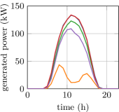
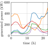
Figure 1: Five examples of power generation profiles generated by the GANs. Left: solar energy, right: wind energy.

V-B Monte Carlo Simulations

To test the proposed framework, we performed $100$ Monte Carlo simulations in which we run Algorithm 1 on different realizations of the energy generation scenarios (i.e., different realizations of $b$).

We considered a microgrid control problem with the following units: $20$ generators, $20$ storages, $60$ controllable loads, $20$ critical loads, $40$ solar generators, $15$ wind generators and the connection to the main grid. For each instance of the problem, we extracted $R=5$ scenarios and fixed a $24$-hour prediction horizon and $1$-hour sampling time. The initial conditions of storages and generators are generated randomly. As regards the load profiles and the daily spot prices, we utilized the data provided by [21], which are shown in Figure 4. We then executed Algorithm 1 for $500$ iterations with a piece-wise constant step size that we initialize to $3.0$ and multiply by $0.5$ every $100$ iterations.

The results of the simulations are shown in Figures 2 and 3. In Figure 2, we plot the cost of the mixed-integer solution computed by the algorithm throughout its evolution (in particular the cost function of the two-stage problem (13)). The picture highlights how the algorithm improves the cost at each iteration, i.e., the more iterations are performed, the more the solution performance improves.

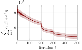
Figure 2: Evolution of the cost yielded by Algorithm 1. The solid line is the mean value of the Monte Carlo trials while the dashed area represents one standard deviation.

In Figure 3, we show the value of the coupling constraints for the two-stage problem (13). The red and green lines correspond to the maximum value of $\eta_{+}$ and $\eta_{-}$ (with changed sign) respectively, where the maximum is taken with respect to the scenarios, to the components of the constraint and to the Monte Carlo trials. The blue line represents the average value of the power balance constraint, while the dashed area corresponds to one standard deviation of the Monte Carlo trials. At each time step the power balance constraints are always in between the upper and lower line, while the uncertainty range reduces as the algorithm progresses.

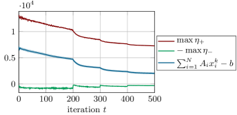
Figure 3: Evolution of the coupling constraint value throughout the evolution of Algorithm 1. The blue line represents the average value of the power balance constraint (the dashed area corresponds to one standard deviation). The upper and lower lines are the maximum positive and negative two-stage violations of the constraints.

V-C Results on a Single Instance

To conclude this section, we show how Algorithm 1 behaves on a single instance of the Monte Carlo trials. In Figure 5, we show the total consumed power and the total curtailed power. In Figure 6, we show the total power exchanged with storage units (a positive value means that, overall, the storage units are charging) and the global level of stored power. The solution provided by the algorithm is such that storages accumulate as much energy as they can during the peaks of power produced by the renewables. This energy is then released during the subsequent hours of the day. In Figure 7, we show the total power exchanged with the utility grid (a positive value means that power is purchased from the grid). Note that, during the peak of power produced by the renewables, the microgrid exports energy to the main grid in order to maximize the income. In Figure 8, we show where does the total available power comes from. In particular we highlight the fraction of power coming from generators, renewables and the utility grid. In this simulation, the generators did not produce any energy.

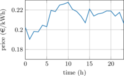
Figure 4: Daily spot prices from Open Power System Data [21].

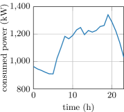
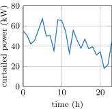
Figure 5: Total consumed power (critical and controllable loads) and curtailed power (for controllable loads only).

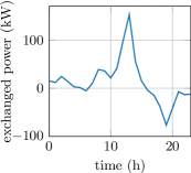
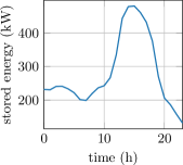
Figure 6: Total average power exchanged by storage units (left) and level of total stored power (right).

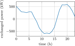
Figure 7: Total power exchanged with the utility grid.

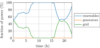
Figure 8: Fraction of consumed power coming from generators, renewables and utility grid at each time slot.

VI Conclusions

In this paper, we considered a microgrid control problem to be solved over a peer-to-peer network of agents. Each agent represents a unit of the microgrid and must cooperate with the other units in order to solve the problem without a centralized coordinator. We used a challenging stochastic mixed-integer microgrid model and proposed a distributed algorithm to solve the problem, for which we provided theoretical guarantees on the constraint violation. Numerical computations on a synthesized problem using Generative Adversarial Networks show the validity of the proposed approach.

-A Review of Primal Decomposition

Consider a network of $N$ agents indexed by $\mathbb{I}=\{1,\ldots,N\}$ that aim to solve a linear program of the form

$$\begin{split}\min_{x_{1},\ldots,x_{N}}\>&\>\sum_{i=1}^{N}c_{i}^{\top}x_{i}\\ \textnormal{subj. to}\>&\>x_{i}\in X_{i},\hskip 28.45274pt\forall i\in\mathbb{I},\\ &\>\sum_{i=1}^{N}A_{i}x_{i}\leq b,\end{split}$$ (22)

where each $x_{i}\in^{n_{i}}$ is the $i$-th optimization variable, $c_{i}\in^{n_{i}}$ is the $i$-th cost vector, $X_{i}\subset^{n_{i}}$ is the $i$-th polyhedral constraint set and $A_{i}\in^{S\times n_{i}}$ is a matrix for the $i$-th contribution to the coupling constraint $\sum_{i=1}^{N}A_{i}x_{i}\leq b\in^{S}$. Problem (22) enjoys the constraint-coupled structure [3] and can be recast into a master-subproblem architecture by using the so-called primal decomposition technique [26]. The right-hand side vector $b$ of the coupling constraint is interpreted as a given (limited) resource to be shared among the network agents. Thus, local allocation vectors $y_{i}\in^{S}$ for all $i$ are introduced such that $\sum_{i=1}^{N}y_{i}=b$. To determine the allocations, a master problem is introduced

$$\begin{split}\min_{y_{1},\ldots,y_{N}}\>&\>\sum_{i=1}^{N}p_{i}(y_{i})\\ \textnormal{subj. to}\>&\>\textstyle\sum\limits_{i=1}^{N}y_{i}=b\\ &\>y_{i}\in Y_{i},\hskip 28.45274pt\forall i\in\mathbb{I},\end{split}$$ (23)

where, for each $i\in\mathbb{I}$, the function $p_{i}:^{S}\rightarrow$ is defined as the optimal cost of the $i$-th (linear programming) subproblem

$$\begin{split}p_{i}(y_{i})=\>\min_{x_{i}}\>&\>c_{i}^{\top}x_{i}\\ \textnormal{subj. to}\>&\>A_{i}x_{i}\leq y_{i}\\ &\>x_{i}\in X_{i}.\end{split}$$ (24)

In problem (23), the new constraint set $Y_{i}\subseteq^{S}$ is the set of $y_{i}$ for which problem (24) is feasible, i.e., such that there exists $x_{i}\in X_{i}$ satisfying the local allocation constraint $A_{i}x_{i}\leq y_{i}$. Assuming problem (22) is feasible and $X_{i}$ are compact sets, if $(y_{1}^{\star},\ldots,y_{N}^{\star})$ is an optimal solution of (23) and, for all $i$, $x_{i}^{\star}$ is optimal for (24) (with $y_{i}=y_{i}^{\star}$), then $(x_{1}^{\star},\ldots,x_{N}^{\star})$ is an optimal solution of the original problem (22) (see, e.g., [26, Lemma 1]).

-B Proof of Theorem IV.5

By the optimality of $(x^{\infty}_{i},\eta^{\infty}_{i})$ for problem (21), it holds

$$c_{i}^{\top}x^{\infty}_{i}+d^{\top}\eta^{\infty}_{i}\leq c_{i}^{\top}x_{i}+d^{\top}\eta_{i}$$ (25)

for all $x_{i}\in X_{i}$ and $\eta_{i}\geq 0$ such that $A_{i}x^{\infty}_{i}\leq y_{i}^{\textsc{lp}}+\eta_{i}$. One vector satisfying such condition is $(x^{\textsc{L}}_{i},\eta^{\textsc{L}}_{i})$ optimal solution of

$$\begin{split}\min_{x_{i},\eta_{i}}\>&\>c_{i}^{\top}x_{i}+d^{\top}\eta_{i}\\ \textnormal{subj. to}\>&\>0\leq\eta_{i}\leq M\mathds{1},\>\>x_{i}\in X_{i},\\ &\>H_{i}x_{i}\leq\ell_{i}+\eta_{i},\end{split}$$ (26)

Indeed, it holds $H_{i}x^{\textsc{L}}_{i}\leq\ell_{i}+\eta^{\textsc{L}}_{i}\leq y_{i}^{\textsc{lp}}+\eta^{\textsc{L}}_{i}$, where the first inequality is by construction and the second one follows by the discussion above on $\ell_{i}$. Thus, by using (25) we conclude that

$$d^{\top}\eta^{\infty}_{i}\leq c_{i}^{\top}(x^{\textsc{L}}_{i}-x^{\infty}_{i})+d^{\top}\eta^{\textsc{L}}_{i}.$$ (27)

By explicitly writing the scalar product $d^{\top}\eta^{\infty}_{i}$ and by using the fact that $d,\eta\geq 0$ we obtain

$$d^{\top}\eta^{\infty}_{i}=\sum_{j=1}^{2RK}d_{j}\eta^{\infty}_{ij}\geq\underbrace{\Big{(}\min_{j\in\{1,\ldots,2RK\}}d_{j}\Big{)}}_{d^{\textsc{min}}}\sum_{j=1}^{2RK}\eta^{\infty}_{ij}.$$

Moreover, by using the fact that $\eta^{\infty}_{ij}\leq\sum_{k=1}^{2RK}\eta^{\infty}_{ik}$ for all $k$ we obtain

$$\eta^{\infty}_{i}\leq\frac{d^{\top}\eta^{\infty}_{i}}{d^{\textsc{min}}}\mathds{1}\leq\frac{c_{i}^{\top}(x^{\textsc{L}}_{i}-x^{\infty}_{i})+d^{\top}\eta^{\textsc{L}}_{i}}{d^{\textsc{min}}}\mathds{1}.$$

Let us now compute an upper bound of the coupling constraint value, i.e.

$$\sum_{i=1}^{N}H_{i}x^{\infty}_{i}-h \leq\underbrace{\sum_{i=1}^{N}y_{i}^{\textsc{lp}}}_{b}+\sum_{i\in I_{\mathbb{Z}}}\eta_{i}^{\textsc{lp}}+\sum_{i\notin I_{\mathbb{Z}}}\eta^{\infty}_{i}-h$$

$$=\sum_{i\in I_{\mathbb{Z}}}\eta_{i}^{\textsc{lp}}+\sum_{i\notin I_{\mathbb{Z}}}\eta^{\infty}_{i}.$$ (28)

where we used the fact that, by Lemma IV.2, for $i\in I_{\mathbb{Z}}$ it holds $H_{i}x^{\infty}_{i}\leq y_{i}^{\textsc{lp}}+\eta_{i}^{\textsc{lp}}$, while for $i\notin I_{\mathbb{Z}}$ it holds $H_{i}x^{\infty}_{i}\leq y_{i}^{\textsc{lp}}+\eta^{\infty}_{i}$. Thus we finally obtain the bound

$$\sum_{i=1}^{N}H_{i}x^{\infty}_{i}-h \leq\sum_{i\in I_{\mathbb{Z}}}\eta_{i}^{\textsc{lp}}+\sum_{i\notin I_{\mathbb{Z}}}\frac{c_{i}^{\top}(x^{\textsc{L}}_{i}-x^{\infty}_{i})+d^{\top}\eta^{\textsc{L}}_{i}}{d^{\textsc{min}}}\mathds{1}.$$

and the proof follows. $\square$

References

- [1] D. K. Molzahn, F. Dörfler, H. Sandberg, S. H. Low, S. Chakrabarti, R. Baldick, and J. Lavaei, “A survey of distributed optimization and control algorithms for electric power systems,” IEEE Transactions on Smart Grid, vol. 8, no. 6, pp. 2941–2962, 2017.
- [2] A. Nedić and J. Liu, “Distributed optimization for control,” Annual Review of Control, Robotics, and Autonomous Systems, vol. 1, pp. 77–103, 2018.
- [3] G. Notarstefano, I. Notarnicola, and A. Camisa, “Distributed optimization for smart cyber-physical networks,” Foundations and Trends® in Systems and Control, vol. 7, no. 3, pp. 253–383, 2019.
- [4] A. Ouammi, H. Dagdougui, L. Dessaint, and R. Sacile, “Coordinated model predictive-based power flows control in a cooperative network of smart microgrids,” IEEE Transactions on Smart grid, vol. 6, no. 5, pp. 2233–2244, 2015.
- [5] S. R. Cominesi, M. Farina, L. Giulioni, B. Picasso, and R. Scattolini, “A two-layer stochastic model predictive control scheme for microgrids,” IEEE Transactions on Control Systems Technology, vol. 26, no. 1, pp. 1–13, 2017.
- [6] C. Le Floch, S. Bansal, C. J. Tomlin, S. J. Moura, and M. N. Zeilinger, “Plug-and-play model predictive control for load shaping and voltage control in smart grids,” IEEE Transactions on Smart Grid, vol. 10, no. 3, pp. 2334–2344, 2017.
- [7] A. Zakariazadeh, S. Jadid, and P. Siano, “Smart microgrid energy and reserve scheduling with demand response using stochastic optimization,” International Journal of Electrical Power & Energy Systems, vol. 63, pp. 523–533, 2014.
- [8] T. A. Nguyen and M. L. Crow, “Stochastic optimization of renewable-based microgrid operation incorporating battery operating cost,” IEEE Transactions on Power Systems, vol. 31, no. 3, pp. 2289–2296, 2015.
- [9] P. O. Kriett and M. Salani, “Optimal control of a residential microgrid,” Energy, vol. 42, no. 1, pp. 321–330, 2012.
- [10] M. Marzband, M. Ghadimi, A. Sumper, and J. L. Domínguez-García, “Experimental validation of a real-time energy management system using multi-period gravitational search algorithm for microgrids in islanded mode,” Applied Energy, vol. 128, pp. 164–174, 2014.
- [11] E. Shirazi and S. Jadid, “Cost reduction and peak shaving through domestic load shifting and DERs,” Energy, vol. 124, pp. 146–159, 2017.
- [12] A. Parisio, E. Rikos, and L. Glielmo, “A model predictive control approach to microgrid operation optimization,” IEEE Transactions on Control Systems Technology, vol. 22, no. 5, pp. 1813–1827, 2014.
- [13] ——, “Stochastic model predictive control for economic/environmental operation management of microgrids: an experimental case study,” Journal of Process Control, vol. 43, pp. 24–37, 2016.
- [14] F. Dörfler, S. Bolognani, J. W. Simpson-Porco, and S. Grammatico, “Distributed control and optimization for autonomous power grids,” in IEEE European Control Conference (ECC). IEEE, 2019, pp. 2436–2453.
- [15] S. Bolognani and S. Zampieri, “A distributed control strategy for reactive power compensation in smart microgrids,” IEEE Transactions on Automatic Control, vol. 58, no. 11, pp. 2818–2833, 2013.
- [16] V. Causevic, A. Falsone, D. Ioli, and M. Prandini, “Energy management in a multi-building set-up via distributed stochastic optimization,” in IEEE Annual American Control Conference (ACC). IEEE, 2018, pp. 5387–5392.
- [17] F. Belluschi, A. Falsone, D. Ioli, K. Margellos, S. Garatti, and M. Prandini, “Distributed optimization for structured programs and its application to energy management in a building district,” Journal of Process Control, vol. 89, pp. 11–21, 2020.
- [18] G. Cavraro, A. Bernstein, R. Carli, and S. Zampieri, “Distributed minimization of the power generation cost in prosumer-based distribution networks,” in IEEE American Control Conference (ACC). IEEE, 2020, pp. 2370–2375.
- [19] A. Falsone, K. Margellos, and M. Prandini, “A distributed iterative algorithm for multi-agent MILPs: finite-time feasibility and performance characterization,” IEEE Control Systems Letters, vol. 2, no. 4, pp. 563–568, 2018.
- [20] A. Camisa, I. Notarnicola, and G. Notarstefano, “Distributed primal decomposition for large-scale MILPs,” IEEE Transactions on Automatic Control, pp. 1–1, 2021.
- [21] OPSD, “Open Power System Data Time Series,” 2020, https://data.open-power-system-data.org/time_series, October 6th, 2020.
- [22] A. Bemporad and M. Morari, “Control of systems integrating logic, dynamics, and constraints,” Automatica, vol. 35, no. 3, pp. 407–427, 1999.
- [23] S. Boyd, S. P. Boyd, and L. Vandenberghe, Convex optimization. Cambridge university press, 2004.
- [24] F. Farina, A. Camisa, A. Testa, I. Notarnicola, and G. Notarstefano, “DISROPT: A Python framework for distributed optimization,” in IFAC World Congress, 2020.
- [25] I. J. Goodfellow, J. Pouget-Abadie, M. Mirza, B. Xu, D. Warde-Farley, S. Ozair, A. Courville, and Y. Bengio, “Generative adversarial networks,” arXiv preprint arXiv:1406.2661, 2014.
- [26] G. J. Silverman, “Primal decomposition of mathematical programs by resource allocation: I–basic theory and a direction-finding procedure,” Operations Research, vol. 20, no. 1, pp. 58–74, 1972.